Formal Derivations of Mode Coupling Equations in Underwater Acoustics: How the Method of Multiple Scales Results in an Expansion over Eigenfunctions and the Vectorized WKBJ Solution for the Amplitudes

Abstract

In this study formal derivation of mode coupling equations in underwater acoustics is revisited. This derivation is based on the method of multiple scales from which modal expansion of the field emerges, and the vectorized WKBJ equation for the coefficients in this expansion are obtained in an automatic way. Asymptotic analysis accomplished in this work also establishes a connection between coupled mode parabolic equations in three-dimensional case and the generalized WKBJ solution that emerges as its two-dimensional counterpart. Despite the fact that similar mode coupling equations can be found in literature, in our study a new systematic and formalized approach to their derivation is proposed. A theorem that guarantees asymptotic conservation of the energy flux in the considered two-dimensional waveguide is also proven.

1. Introduction

The normal mode representation of acoustic field is often used in underwater acoustics. This representation is obtained by local separation of variables in the original boundary value problem for the Helmholtz equation for acoustic pressure. Within any cross-section of the waveguide the vertical distribution of sound pressure is represented in the form of a series over eigenfunctions of certain Sturm-Liouville problem [1,2]. These eigenfunctions are often called normal modes, while the coefficients of the field expansion over a basis formed by them are called mode amplitudes.

The standard textbook approach to the derivation of equations for mode amplitudes [1,3,4,5] consists of the staircase approximation and matching of field expansions at two range-independent sections of the waveguide. This matching eventually results in a large system of linear equations where unknowns are expansion coefficients at all sections (steps) of the staircase. Other approaches reported in some studies [2,6,7,8] are free from the staircase approximation and result in “continuously coupled” systems of ordinary differential equations for mode amplitudes.

In this study we revisit the derivation of such equations using two different asymptotic approximations, namely the method of multiple scales [9,10] and the vectorized WKBJ approach [11,12] (the abbreviation stands for Wentzel–Kramers–Brillouin-Jeffrys method emerging from quantum mechanics, see [13]). It can be seen from this article that in fact a very formal multi-scale derivation implicitly incorporates both the modal expansion of the field and the WKBJ approximation for the mode amplitudes. The latter fact is in interesting observation per se, as it allows to resolve various issues arising throughout the derivation with greater flexibility. For example, in this study we show that the attenuation can be taken into account by including additional terms into the coupling equations instead of more straightforward way of handling it via the imaginary parts of the horizontal wavenumbers. Similar techniques can be used, e.g., also to tackle weak elasticity effects in the bottom [14] and many other possible complications [15].

For the obtained equations an important property of the asymptotic acoustic energy flux [6,8] conservation is proved (see the definition and discussion in Section 5). The respective theorem guarantees that energy flux is conserved within the considered asymptotic solutions modulo the terms of higher order with respect to the small parameter used in the derivation (by contrast to acoustic Helmholtz equation that satisfies the property of the energy flux conservation exactly).

Furthermore, the use of asymptotic methods outlined here allows to establish a bridge between the mode coupling equations in a 2D waveguide and the 3D solutions obtained in the framework of the so-called mode parabolic equations theory [10,16] (in fact, the latter equations reduce to the mode coupling equations derived here if the derivatives with respect to the transverse horizontal variable vanish).

2. Problem Formulation

Let us consider time-harmonic sound propagation in an axially symmetric three-dimensional waveguide $\mathsf{\Omega }=\left\{\right(r,\theta ,z\left)\right|0\le r<\infty ,0\le \theta <2\pi ,0\le z\le H\}$ (where z-axis is directed downwards) that is described by the acoustic Helmholtz equation

$${\left(\gamma P_r\right)}_r+\frac{1}{r}\gamma P_r+{\left(\gamma P_z\right)}_z+\gamma {\kappa }^{2}P=\frac{-\gamma \delta (z-z_s)\delta \left(r\right)}{2\pi r},$$

(1)

where $\gamma =1/\rho$ is inverse to the density $\rho =\rho (r,z)$, $\kappa (r,z)=\frac{\omega }{c(r,z)}$ is the medium wavenumber (here $\omega$ is the cyclic frequency, and $c=c(r,z)$ is the sound speed). Throughout this study subscripts $r,z$ denote partial derivatives with respect to these variables.

We also assume that suitable radiation conditions are imposed at infinity in the $r,\theta$ plane [17,18]. At the sea surface $z=0$ a pressure-release boundary condition

$$\begin{array}{c}P=0\mathrm{at}z=0,\end{array}$$

(2)

is set up, while a rigid-wall boundary condition

$$\partial P/\partial z=0\mathrm{at}z=H,$$

(3)

is imposed at a subbottom (i.e., H is a sufficiently large value of depth at which the computational domain is truncated). The parameters of the media may exhibit finite-jump discontinuities at the non-intersecting smooth interfaces $z=h_1\left(r\right),\dots ,h_m\left(r\right)$, where the usual continuity conditions

$$\begin{array}{c}\begin{array}{cc}& P_{+}=P_{-},\hfill \\ & {\gamma }_{+}{\left(P_z-h_r{P}_r\right)}_{+}={\gamma }_{-}{\left(P_z-h_r{P}_r\right)}_{-}\hfill \end{array}\end{array}$$

(4)

for acoustic pressure and particle velocity are imposed. Hereinafter we use the notations $f{(z_0,r)}_{+}={\lim }_{z\downarrow z_0}f(z,r)$ and $f{(z_0,r)}_{-}={\lim }_{z\uparrow z_0}f(z,r)$ for the quantities just below and above such interfaces.

Without loss of generality we can consider the case $m=1$ and denote $h_1$ by h (dropping the subscript).

It is well known that for any given r the solution of Equation (1) can be represented in the form of a series over eigenfunctions ${\varphi }_j(z,r)$ of the following Sturm-Liouville problem [1]

$$\left\{\begin{array}{c}{\left(\gamma {\varphi }_z\right)}_z+\gamma \frac{{\omega }^2}{c^2}\varphi =\gamma k^2\varphi =0,\hfill \\ \varphi \left(0\right)=0,\hfill \\ {\varphi }_z\left(H\right)=0,\hfill \\ {\varphi }_{+}={\varphi }_{-},\hfill \\ {\gamma }_{+}{\left({\varphi }_z\right)}_{+}={\gamma }_{-}{\left({\varphi }_z\right)}_{-},\hfill \end{array}\right.$$

(5)

where $k_j\left(r\right)$ are their respective horizontal wavenumbers (note that the eigenvalues are $k_j^2$). Note that the term problem is usually used in this study to refer to some equation complemented by initial or boundary conditions.

Hereafter we always assume that the mode functions are normalized, i.e., that

$$\int \gamma \left(z\right){\varphi }_j\left(z\right){\varphi }_{\ell }\left(z\right)dz={\delta }_{j\ell }$$

(the integration with respect to z withing this study is always performed over the interval $[0,H]$). It is known that all eigenfunctions $\left\{{\varphi }_j(z,r)\right\}$ form an orthogonal basis for a given value of r, i.e., in a given vertical cross-section of the waveguide. We also assume that they are ordered in such a way that $k_j^2>k_{j+1}^2$.

While the set of eigenfunctions is countable due to Dirichlet and Neuman boundary conditions at the ends of the interval $[0,H]$, only finite number of them have positive eigenvalues $k_j^2$. All other eigenvalues $k_j^2$ (starting at sufficiently large j) are negative, and their respective horizontal wavenumbers $k_j$ are imaginary (in fact, the set of eigenvalues $k_j^2$ has $-\infty$ as a single accumulation point [19]). The series over ${\varphi }_j$ is usually truncated in practical applications at some sufficiently large $j=N$.

Note that $k_j$ can be also considered complex. Their imaginary parts result from attenuation of sound waves in the bottom that is taken into account by introducing a small imaginary component of $\omega /c$. Since it is often convenient to keep the problem (5) self-adjoint, one can compute imaginary corrections to the real wavenumbers using perturbation theory after the solution of (5) with real $\omega /c$.

The goal of the present study is to derive an approximate solution of the boundary-value problem (BVP) for the Helmholtz Equation (1) with the boundary conditions given by Equations (2)–(4) (and the radiation conditions at infinity) in terms of a truncated series

$$P(r,z)={\displaystyle \sum _{j=1}^N}{A}_j\left(r\right){\varphi }_j(z,r),$$

(6)

over eigenfunctions of the Sturm-Liouville problem (5). More precisely, the objective is to obtain convenient equations for the coefficients $A_j\left(r\right)$ in Equation (6) that can be easily solved numerically.

It can be shown (see Appendix A) that mode amplitudes $A_j\left(r\right)$ satisfy the following coupled system of equations

$$A_{j,rr}+\frac{1}{r}{A}_{j,r}+k_j^2{A}_j+{\displaystyle \sum _{l=1}^n}{U}_{lj}{A}_l+{\displaystyle \sum _{l=1}^n}(V_{lj}-V_{jl})A_{l,r}=-\frac{1}{2\pi r}\gamma \left(z_s\right){\varphi }_j\left(z_s\right)\delta \left(r\right),$$

(7)

where $U_{lj}=\int \gamma \left({\varphi }_{l,rr}+\frac{1}{r}{\varphi }_{l,r}\right){\varphi }_{j}dz$ and $V_{lj}=\int \gamma {\varphi }_{l,r}{\varphi }_{j}dz$ are elements of the square $N\times N$ matrices $\mathit{U}$ and $\mathit{V}$, respectively. It is widely accepted that in realistic propagation scenarios the coupling terms containing $U_{lj}$ can be neglected (hereafter we drop them).

In a range-independent waveguide when the coupling terms $V_{lj}$ also vanish the solutions of Equation (7) have the form [1]

$$A_{j,0}\left(r\right)=\frac{\mathrm{i}\gamma \left(z_s\right)}{4}{\varphi }_j\left(z_s\right)H_0^{\left(1\right)}\left(k_{j}r\right).$$

(8)

3. The Derivation of the Mode Coupling Equations Using the Vectorized WKBJ Approximation

Since (7) is a coupled system of 2D elliptic equations that should be complemented by radiation boundary conditions (that follow from the respective conditions for Equation (1)), it is not convenient for numerical solution. Indeed, mesh size for any sort of discretization must be such that all waves forming its solution are resolved sufficiently well (e.g., 10–15 points per wavelength) which is often too restrictive. Moreover, such system cannot be solved by a marching schemes that are usually the most convenient and robust. In this section, we use the vectorized form of WKBJ ansatz in order to reduce Equation (7) to an evolutionary-type system of equations that can be solved by a marching scheme on a very coarse grid.

3.1. Vectorized Equations for Mode Amplitudes

The set of N scalar equations (7) can be replaced by a single equation

$$\left(\frac{d^2}{d{r}^2}+\frac{1}{r}\frac{d}{dr}+\mathsf{\Gamma }\left(r\right)\frac{d}{dr}\right)\mathit{a}\left(r\right)+\frac{1}{{ϵ}^2}{\left(\overline{\mathit{K}}\left(r\right)\right)}^2\mathit{a}\left(r\right)=0,$$

(9)

for the unknown vector function $\mathit{a}\left(r\right)={(A_1\left(r\right),A_2\left(r\right),\cdots ,A_n\left(r\right))}^T$ (superscript T denotes transposition), where $\mathsf{\Gamma }=\mathit{V}-{\mathit{V}}^T$, and $\mathit{K}\left(r\right)=\frac{1}{ϵ}\overline{\mathit{K}}\left(r\right)=\mathrm{diag}(k_1\left(r\right),\cdots ,k_n\left(r\right))$ (i.e., $\mathit{K}\left(r\right)$ is a diagonal matrix with eigenvalues $k_j\left(r\right)$ on the main diagonal). Note that we formally introduced a small parameter into the vectorized form Equation (9) of mode coupling equations. Physically it means that typical horizontal wavelength associated with mode amplitudes is much smaller than “horizontal” size of media inhomogeneities.

The BVP for Equation (9) is set in the following way. At certain small range from the source $r=r_0$ we impose the condition $A_j\left(r_0\right)=A_{j,0}\left(r_0\right)$ that represents the wavefield excited by a point source (as if the waveguide in a small vicinity of the source is range-independent).

At $r\to \infty$ we require that partial Sveshnikov-type radiation boundary condition ${\left.\sqrt{r}\left(\frac{d{A}_j}{dr}-k_{j,\infty }{A}_j\right)\right|}_{r\to \infty }=0$ is fulfilled (it is assumed that waveguide properties such as $h,c$, etc. do not depend on r outside sufficiently large cylinder $r\le r_{max}$, and that $k_j\left(r\right)=k_{j,\infty }$ for $r>r_{max}$, i.e., the medium becomes range-independent).

3.2. Vectorized WKBJ Approximation for the Mode Amplitudes

Following [11,12], we introduce into Equation (9) the vectorized WKBJ-ansatz of the form

$$\mathit{a}\left(r\right)=\left(\begin{array}{c}{B}_1\left(r\right){\mathrm{e}}^{\mathrm{i}{\mathsf{\Phi }}_1\left(r\right)/ϵ}\\ B_2\left(r\right){\mathrm{e}}^{\mathrm{i}{\mathsf{\Phi }}_2\left(r\right)/ϵ}\\ ⋮\\ B_N\left(r\right){\mathrm{e}}^{\mathrm{i}{\mathsf{\Phi }}_N\left(r\right)/ϵ}\end{array}\right)=\exp \left(\mathrm{i}\frac{\overline{\mathsf{\Phi }}\left(r\right)}{ϵ}\right)\mathit{b}\left(r\right),$$

(10)

where $\mathsf{\Phi }\left(r\right)=\overline{\mathsf{\Phi }}\left(r\right)/ϵ=\mathrm{diag}({\mathsf{\Phi }}_1\left(r\right)/ϵ,\cdots ,{\mathsf{\Phi }}_N\left(r\right)/ϵ)$, and $\mathit{b}\left(r\right)={(B_1\left(r\right),\cdots ,B_N\left(r\right))}^T$.

Let us now substitute the ansatz (10) into Equation (9)

$$\begin{array}{c}{\mathrm{e}}^{\mathrm{i}\overline{\mathsf{\Phi }}/ϵ}\left(-\frac{{\left({\overline{\mathsf{\Phi }}}_r\right)}^2}{{ϵ}^2}\mathit{b}+\mathrm{i}\frac{{\overline{\mathsf{\Phi }}}_{rr}}{ϵ}\mathit{b}+2\mathrm{i}\frac{{\overline{\mathsf{\Phi }}}_r}{ϵ}{\mathit{b}}_r+{\mathit{b}}_{rr}\right)+\frac{1}{r}{\mathrm{e}}^{\mathrm{i}\overline{\mathsf{\Phi }}/ϵ}\left(\mathrm{i}\frac{{\overline{\mathsf{\Phi }}}_r}{ϵ}\mathit{b}+{\mathit{b}}_r\right)\hfill \\ \hfill +\mathsf{\Gamma }{\mathrm{e}}^{\mathrm{i}\overline{\mathsf{\Phi }}/ϵ}\left(\mathrm{i}\frac{{\overline{\mathsf{\Phi }}}_r}{ϵ}\mathit{b}+{\mathit{b}}_r\right)+\frac{{\overline{\mathit{K}}}^2}{{ϵ}^2}{\mathrm{e}}^{\mathrm{i}\overline{\mathsf{\Phi }}/ϵ}\mathit{b}=0.\end{array}$$

(11)

Now we combine terms of the same order in $ϵ$ (starting with ${ϵ}^{-2}$) and obtain a series of equations similar to the one in the standard WKBJ method (see [11,13]).

For the lowest power of the small parameter we obtain a matrix Hamilton-Jacobi equation of the form

$${\left({\overline{\mathsf{\Phi }}}_r\left(r\right)\right)}^2={\left(\overline{\mathit{K}}\left(r\right)\right)}^2,$$

(12)

and therefore ${\mathsf{\Phi }}_r\left(r\right)=\pm \mathit{K}\left(r\right)$. We choose ${\mathsf{\Phi }}_{\mathit{r}}=\mathit{K}$ thus neglecting back scattering and retaining only waves propagating in outward direction from the source. This assumption is known to be reasonable in underwater acoustics and geophysics, and it leads to substantial simplification of the solution procedure. Collecting the terms of the order ${ϵ}^{-1}$ in Equation (11), we obtain the following equation for the vector-function $\mathit{b}\left(r\right)$

$$2\mathit{K}{\mathit{b}}_r+\frac{1}{r}\mathit{K}\mathit{b}+{\mathit{K}}_r\mathit{b}+{\mathrm{e}}^{-\mathrm{i}\mathsf{\Phi }}\mathsf{\Gamma }{\mathrm{e}}^{\mathrm{i}\mathsf{\Phi }}\mathit{K}\mathit{b}=0.$$

(13)

Since backward propagation is suppressed, we now have a first-order ODE system for envelopes $\mathit{b}\left(r\right)$ of mode amplitudes $\mathit{a}\left(r\right)$. Thus, the original BVP for Equation (9) was replaced by an initial-value problem for Equation (13) with the initial condition $B_j\left(r_0\right)=A_j{r}_0{\mathrm{e}}^{-\mathrm{i}{k}_j\left(0\right)r_0}$. Within this approach the horizontal wavenumbers $k_j\left(r\right)$ can be complex, that is, contain small imaginary component corresponding to the sound attenuation in the propagation media.

Note that the matrix $\mathbf{\Xi }={\mathrm{e}}^{-\mathrm{i}\mathsf{\Phi }\left(r\right)}\mathsf{\Gamma }\left(r\right){\mathrm{e}}^{\mathrm{i}\mathsf{\Phi }\left(r\right)}$ consists of elements of the form

$${\Xi }_{ij}=(V_{ij}-V_{ji}){\mathrm{e}}^{{\mathsf{\Phi }}_j\left(r\right)/ϵ-{\mathsf{\Phi }}_i\left(r\right)/ϵ}.$$

4. The Derivation of the Mode Coupling Equations by the Method of Multiple Scales

In this section we perform the derivation of a coupled mode model of sound propagation by the method of multiple scales [9]. Within this approach modal expansion emerges automatically due to our scaling of the independent variables. However, it will be shown that the final represenation of the acoustic field will be identical to (6), where the mode amplitudes will be obtained from the equations equivalent to (13).

Let us introduce a small parameter $ϵ$ (the ratio of the typical wavelength to the typical size of medium inhomogeneities) and the slow variable $R=ϵr$. We now assume the following expansions for the parameters ${\kappa }^2$, $\gamma$ and h:

$$\begin{array}{c}{\kappa }^2={\kappa }_0^2(R,z)+ϵ\nu (R,z),\gamma =\gamma (R,z),h=h\left(R\right).\end{array}$$

Within this approach we include the attenuation effects by allowing $\nu$ to be complex. More precisely, we take $\mathrm{Im}\nu =2\eta \beta {\kappa }_0$, where $\eta ={\left(40\pi {\log }_{10}e\right)}^{-1}$ and $\beta$ is the attenuation in decibels per wavelength. This implies that $\mathrm{Im}\nu \ge 0$.

Consider a solution to the Helmholtz Equation (1) in the form of the WKBJ-ansatz with two spatial scales

$$\begin{array}{c}P={\displaystyle \sum _{j=1}^N}(u_0^{\left(j\right)}(R,z)+ϵu_1^{\left(j\right)}(R,z)+\dots ){\mathrm{e}}^{\mathrm{i}{\mathsf{\Phi }}_j/ϵ}.\end{array}$$

(14)

where $\left\{{\mathsf{\Phi }}_j\right|j=1,\cdots ,N\}$ is a set of phases (fast variables). In fact, we even have three variability scales: fast oscillatory phases $\mathsf{\Phi }$, “normal” variable z and “slow” variable R.

Introducing this ansatz into Equation (1), boundary condition (2) and interface conditions (4) (all rewritten in the slow variable), we obtain a sequence of the boundary value problems for the terms of each order of $ϵ$.

4.1. The Problem at $O\left({ϵ}^0\right)$

To obtain the normal modes we first consider the ansatz of the form of a zero-order approximation $P=u_0^{\left(j\right)}(R,z){\mathrm{e}}^{\mathrm{i}{\mathsf{\Phi }}_j(R,z)/ϵ}$ (we omit the mode number j where it does not lead to confusion). From the equations at $O\left({ϵ}^{-2}\right)$ and $O\left({ϵ}^{-1}\right)$ we can conclude that $\mathsf{\Phi }$ is independent on z.

At $O\left({ϵ}^0\right)$ now we have

$$\begin{array}{c}{\left(\gamma u_{0z}\right)}_z+\gamma n_0^2-\gamma {\left({\mathsf{\Phi }}_R\right)}^2{u}_0=0,\end{array}$$

(15)

with the interface conditions of the order ${ϵ}^0$

$$\begin{array}{c}\begin{array}{cc}& u_{0+}=u_0-,\hfill \\ & {\left(\gamma \frac{\partial u_0}{\partial z}\right)}_{+}={\left(\gamma \frac{\partial u_0}{\partial z}\right)}_{-}\mathrm{at}z=h,\hfill \end{array}\end{array}$$

(16)

and boundary conditions $u=0$ at $z=0$ and $\partial u/\partial z=0$ at $z=H$. We seek a solution to problem (15) and (16) in the form $u_0=B\left(R\right)\varphi (R,z).$ From Equations (15) and (16) we obtain precisely the spectral problem (5) for the function $\varphi$ with the spectral parameter $k^2={\left({\mathsf{\Phi }}_R\right)}^2$.

4.2. The Derivatives of Eigenfunctions and Wavenumbers with Respect to R

Before considering the equality for the terms of the order $O\left({ϵ}^1\right)$ we should discuss the calculation of the derivatives of the eigenfunctions and wavenumbers with respect to R. Perturbation theory for acoustic modes in the case of water depth variations was developed in [20,21]. Equivalent but somewhat different first-order formulae we also derived in [6,10]. Here we obtain them in yet another way more consistent with the coupled mode theory.

Differentiating spectral problem (5) with respect to R, we obtain the boundary value problem for ${\varphi }_{jR}$

$$\begin{array}{c}\begin{array}{cc}& {\left(\gamma {\varphi }_{jRz}\right)}_z+\gamma {\kappa }_0^2{\varphi }_{jR}-\gamma k_j^2{\varphi }_{jR}=-{\left({\gamma }_R{\varphi }_{jz}\right)}_z-\hfill \\ & {\left(\gamma {\kappa }_0^2\right)}_R{\varphi }_j+2k_{jR}{k}_j\gamma {\varphi }_j+{\gamma }_R{k}_j^2{\varphi }_j,\hfill \\ & {\varphi }_{jR}\left(0\right)=0,{\varphi }_{jRz}\left(H\right)=0,\hfill \end{array}\end{array}$$

(17)

with interface conditions at $z=h$

$$\begin{array}{c}\begin{array}{cc}& {\varphi }_{jR+}-{\varphi }_{jR-}=-h_R({\varphi }_{jz+}-{\varphi }_{jz-}),\hfill \\ & {\gamma }_{+}{\varphi }_{jRz+}-{\gamma }_{-}{\varphi }_{jRz-}=-\left({\gamma }_{R+}{\varphi }_{jz+}-\right.\hfill \\ & \left.{\gamma }_{R-}{\varphi }_{jz-}\right)-h_R\left({\left({\left(\gamma {\varphi }_{jz}\right)}_z\right)}_{+}-{\left({\left(\gamma {\varphi }_{jz}\right)}_z\right)}_{-}\right).\hfill \end{array}\end{array}$$

(18)

The solution to the problem (17) and (18) is sought in the form

$$\begin{array}{c}{\varphi }_{jR}={\displaystyle \sum _{l=0}^{\infty }}{\overline{V}}_{jl}{\varphi }_l,\mathrm{where}{\overline{V}}_{jl}=V_{jl}/ϵ={\int }_0^H\gamma {\varphi }_{jR}{\varphi }_{l}dz.\end{array}$$

Multiplying (17) by ${\varphi }_l$ and then integrating resulting equation from 0 to H by parts twice with the use of interface conditions (18), we obtain

$$\begin{array}{c}\begin{array}{cc}& \left(k_l^2-k_j^2\right){\overline{V}}_{jl}={\int }_0^H{\gamma }_R{\varphi }_{jz}{\varphi }_{lz}dz+2k_{jR}{k}_j{\delta }_{jl}-\hfill \\ & -{\int }_0^H{\left(\gamma {\kappa }_0^2\right)}_R{\varphi }_j{\varphi }_{l}dz+k_j^2{\int }_0^H{\gamma }_R{\varphi }_j{\varphi }_{l}dz+\hfill \\ & \left\{h_R{\left({\gamma }^2{\varphi }_{jz}{\varphi }_{lz}\right)}_{+}\left[{\left(\frac{1}{\gamma }\right)}_{+}-{\left(\frac{1}{\gamma }\right)}_{-}\right]-\right.\hfill \\ & {\left.\left.h_R{\varphi }_j{\varphi }_l\left[{\left(\gamma \left(k_j^2-{\kappa }_0^2\right)\right)}_{+}-{\left(\gamma \left(k_j^2-{\kappa }_0^2\right)\right)}_{-}\right]\phantom{\frac{1}{\gamma }}\right\}\right|}_{z=h},\hfill \end{array}\end{array}$$

where ${\delta }_{jl}$ is the Kronecker delta. From the latter equality the coefficients $V_{jl}$ can be easily obtained for $j\ne l$. Note that ${\left({\gamma }^2{\varphi }_{jz}{\varphi }_{lz}\right)}_{+}={\left({\gamma }^2{\varphi }_{jz}{\varphi }_{lz}\right)}_{-}$.

The formula for coefficients $V_{jj}$ can be obtained by differentiating the normalization condition for the modes

$$\begin{array}{cc}\hfill & {\left({\int }_0^H\gamma {\varphi }_j^{2}dz\right)}_R={\left({\int }_h^H\gamma {\varphi }_j^{2}dz+{\int }_0^h\gamma {\varphi }_j^{2}dz\right)}_R=\hfill \\ \hfill & ={\int }_0^H{\gamma }_R{\varphi }_j^{2}dz+2{\int }_0^H\gamma {\varphi }_{jR}{\varphi }_{j}dz+h_R{\varphi }_j^2{\left.\left[{\gamma }_{-}-{\gamma }_{+}\right]\right|}_{z=h}=0.\hfill \end{array}$$

(19)

From the latter equality we find that

$$2{\overline{V}}_{jj}=-{\int }_0^H{\gamma }_R{\varphi }_j^{2}dz+h_R{\varphi }_j^2{\left.\left[{\gamma }_{+}-{\gamma }_{-}\right]\right|}_{z=h}.$$

(20)

4.3. The Problem at $O\left({ϵ}^1\right)$

We now represent a solution to the Helmholtz Equation (1) in the form of ansatz (14). At $O\left({ϵ}^1\right)$ we obtain

$$\begin{array}{c}\begin{array}{cc}& {\displaystyle \sum _{j=1}^N}\left({\left(\gamma u_{1z}^{\left(j\right)}\right)}_z+\gamma {\kappa }_0^2{u}_1^{\left(j\right)}-\gamma k_j^2{u}_1^{\left(j\right)}\right){\mathrm{e}}^{\mathrm{i}{\mathsf{\Phi }}_j/ϵ}=\hfill \\ & {\displaystyle \sum _{j=1}^N}\left(-\mathrm{i}{\gamma }_R{k}_j{u}_0^{\left(j\right)}-2\mathrm{i}\gamma k_j{u}_{0R}^{\left(j\right)}-\mathrm{i}\gamma k_{jR}{u}_0^{\left(j\right)}-\mathrm{i}\gamma k_j\frac{1}{R}{u}_0^{\left(j\right)}-\nu \gamma u_0^{\left(j\right)}\right){\mathrm{e}}^{\mathrm{i}{\mathsf{\Phi }}_j/ϵ},\hfill \end{array}\end{array}$$

(21)

with the boundary conditions $u_1^{\left(j\right)}=0$ at $z=0$, $\partial u_1^{\left(j\right)}/\partial z=0$ at $z=H$, and the interface conditions at $z=h\left(R\right)$:

$$\begin{array}{c}\begin{array}{cc}& {\displaystyle \sum _{j=1}^N}(u_{1+}^{\left(j\right)}-u_{1-}^{\left(j\right)}){\mathrm{e}}^{\mathrm{i}{\mathsf{\Phi }}_j/ϵ}=0,\hfill \\ & {\displaystyle \sum _{j=1}^N}[{\gamma }_{+}{u}_{1z+}^{\left(j\right)}-{\gamma }_{-}{u}_{1z-}^{\left(j\right)}+\mathrm{i}{k}_j{h}_R{u}_0^{\left(j\right)}({\gamma }_{-}-{\gamma }_{+})]{\mathrm{e}}^{\mathrm{i}{\mathsf{\Phi }}_j/ϵ}=0.\hfill \end{array}\end{array}$$

(22)

We seek a solution to problem (21) and (22) in the form

$$u_1^{\left(j\right)}={\displaystyle \sum _{l=0}^{\infty }}{Q}_{jl}(X,Y){\varphi }_l(z,X),where{Q}_{jl}={\int }_0^H\gamma u_1^{\left(j\right)}{\varphi }_{l}dz.$$

Multiplying (21) by ${\varphi }_l$ and then integrating resulting equation from 0 to H by parts twice with the use of interface conditions (22), we obtain

$$\begin{array}{c}\begin{array}{cc}& {\displaystyle \sum _{j=1}^N}\left((k_l^2-k_j^2)Q_{jl}-{\left.B_j\mathrm{i}{k}_j{h}_R{\varphi }_j{\varphi }_l\left[{\gamma }_{+}-{\gamma }_{-}\right]\right|}_{z=h}\right){\mathrm{e}}^{\mathrm{i}{\mathsf{\Phi }}_j/ϵ}\hfill \\ & ={\displaystyle \sum _{j=1}^N}\left(-\mathrm{i}{k}_j{B}_j{\int }_0^H{\gamma }_R{\varphi }_j{\varphi }_{l}dz-2\mathrm{i}{k}_j{B}_j{\int }_0^H\gamma {\varphi }_{jR}{\varphi }_{l}dz-2\mathrm{i}{k}_j{B}_{j,R}{\int }_0^H\gamma {\varphi }_j{\varphi }_{l}dz\right.\hfill \\ & \left.-\mathrm{i}{k}_{j,R}{B}_j{\int }_0^H\gamma {\varphi }_j{\varphi }_{l}dz-\mathrm{i}{k}_j\frac{1}{R}{B}_j{\int }_0^H\gamma {\varphi }_j{\varphi }_{l}dz-B_j{\int }_0^H\nu \gamma {\varphi }_j{\varphi }_{l}dz\right){\mathrm{e}}^{\mathrm{i}{\mathsf{\Phi }}_j/ϵ}.\hfill \end{array}\end{array}$$

The terms $(k_l^2-k_j^2)Q_{jl}$ in these expressions can be omitted because of the resonant condition $|k_l-k_j|=O\left(ϵ\right)$. Since

$$-\mathrm{i}{k}_j{B}_j{\int }_0^H{\gamma }_R{\varphi }_j{\varphi }_{l}dz-2\mathrm{i}{k}_j{B}_j{\int }_0^H\gamma {\varphi }_{jR}{\varphi }_{l}dz=\mathrm{i}{k}_j{B}_j\left({\overline{V}}_{lj}-{\overline{V}}_{jl}\right)-\mathrm{i}{k}_j{B}_j{h}_R{\varphi }_j{\varphi }_l{\left.\left[{\gamma }_{+}-{\gamma }_{-}\right]\right|}_{z=h},$$

we get, after some algebra,

$$\begin{array}{c}\begin{array}{cc}& {\displaystyle \sum _{j=1}^N}\left(\phantom{{\int }_0^H\nu \gamma {\varphi }_j{\varphi }_{l}dz}\mathrm{i}{k}_j{B}_j\left({\overline{V}}_{lj}-{\overline{V}}_{jl}\right)-2\mathrm{i}{k}_j{B}_{j,R}{\delta }_{jl}-\mathrm{i}{k}_{jR}{B}_j{\delta }_{jl}\right.\hfill \\ & \left.-\mathrm{i}{k}_j\frac{1}{R}{B}_j{\delta }_{jl}-B_j{\int }_0^H\nu \gamma {\varphi }_j{\varphi }_{l}dz\right){\mathrm{e}}^{\mathrm{i}{\mathsf{\Phi }}_j/ϵ}=0.\hfill \end{array}\end{array}$$

The results obtained so far can be summarized as follows.

Proposition 1.

The solvability condition for the problem at $O\left({ϵ}^1\right)$ is expressed by the system of equations for $l=1,\dots ,N$

$$\begin{array}{c}2\mathrm{i}{k}_l{B}_{l,R}+\mathrm{i}{k}_{l,R}{B}_l+\mathrm{i}{k}_l\frac{1}{R}{B}_l+{\displaystyle \sum _{j=1}^N}{\alpha }_{lj}{B}_j{\mathrm{e}}^{{\mathsf{\Phi }}_{lj}}=0,\end{array}$$

(23)

where ${\alpha }_{lj}$ and ${\mathsf{\Phi }}_{lj}$ are given by the following formulas

$$\begin{array}{c}\begin{array}{cc}& {\alpha }_{lj}={\int }_0^H\gamma \nu {\varphi }_j{\varphi }_{l}dz-\mathrm{i}{k}_j\left({\overline{V}}_{lj}-{\overline{V}}_{jl}\right),\hfill \\ & {\mathsf{\Phi }}_{lj}=\frac{\mathrm{i}}{ϵ}({\mathsf{\Phi }}_j-{\mathsf{\Phi }}_l).\hfill \end{array}\end{array}$$

(24)

Rewriting Equations (23) and (24) in physical variables (r instead of R) and combining them into one equation for a vector-function $\mathit{b}\left(r\right)$ we obtain Equation (13) from the previous section (modulo the attenuation-related term in Equation (24)).

5. Energy Flux Conservation in Approximate Solution Obtained by Integrating the Equations for Mode Amplitudes

Energy flux conservation is widely considered an important property for various propagation models in underwater acoustics [22]. It indicated the consistency of various approximations used in the derivation with basic physical laws. Indeed, the Helmholtz equation enjoys this property, and in fact it follows from the energy conservation law for the wave equation [23].

For time-harmonic waves of the angular frequency $\omega$ acoustic energy flux averaged over the period is defined as

$$J(r,z)=\frac{1}{2\omega }\gamma \mathrm{Im}\left(\left(\mathrm{grad}P(r,z)\right)P^{*}(r,z)\right).$$

From now on we drop the inessential factor $1/2\omega$. As it is well known, if P is a solution of the Helmholtz Equation (1) then the corresponding energy flux is conserved, that is $\mathrm{div}J(r,z)=0.$ With our boundary conditions we have also the conservation property

$$\mathrm{div}{\int }_0^{H}J(r,z)dz=0.$$

Proposition 2.

Assume that $\mathrm{Im}\overline{\nu }=0$. Let $\left\{B_j\right|j=1,\dots N\}$ be a solution to Equation (23). Then for $P={\displaystyle \sum _{j=1}^N}{B}_j{\varphi }_j{\mathrm{e}}^{\mathrm{i}{\mathsf{\Phi }}_j/ϵ}$ we have $\mathrm{div}{\int }_0^{H}J(r,z)dz=O\left({ϵ}^2\right).$

Proof. 

First calculate the divergence in the general form for the used representation of the field

$$\begin{array}{l}\mathrm{div}{\int }_0^{H}J(r,z)dz\\ =\frac{1}{r}\frac{\partial }{\partial r}\left\{r\left[{\displaystyle \sum _{l=1}^N}{k}_l{\left|B_l\right|}^2\right.\right.+ϵ{\displaystyle \sum _{l=1}^N}{\displaystyle \sum _{j=1}^N}\mathrm{Im}\left({\overline{V}}_{lj}{B}_l{B}_j^{*}{\mathrm{e}}^{\mathrm{i}({\mathsf{\Phi }}_l-{\mathsf{\Phi }}_j)/ϵ)}\right)\left.\left.+ϵ{\displaystyle \sum _{l=1}^N}\mathrm{Im}\left(B_{l,R}{B}_l^{*}\right)\right]\right\}\hfill \\ =ϵ{\displaystyle \sum _{l=1}^N}{\displaystyle \sum _{j=1}^N}(k_l-k_j){\overline{V}}_{lj}\mathrm{Re}\left(B_j{B}_l^{*}{\mathrm{e}}^{\mathrm{i}({\mathsf{\Phi }}_j-{\mathsf{\Phi }}_l)/ϵ)}\right)+ϵ{\displaystyle \sum _{l=1}^N}{\left(k_l{\left|B_l\right|}^2\right)}_R+ϵ\frac{1}{R}{\displaystyle \sum _{l=1}^N}{k}_l{\left|B_l\right|}^2+O\left({ϵ}^2\right)\hfill \end{array}$$

(25)

Consider now the sum on l of Equation (23) multiplied by $B_l^{*}$ minus the conjugate equations multiplied by $B_l$

$$\begin{array}{c}{\displaystyle \sum _{l=1}^N}\left[\left(2\mathrm{i}{k}_l{B}_{l,R}+\mathrm{i}{k}_{l,R}{B}_l+\mathrm{i}{k}_l\frac{1}{R}{B}_l+{\displaystyle \sum _{j=1}^N}{\alpha }_{lj}{B}_j{\mathrm{e}}^{{\mathsf{\Phi }}_{lj}}\phantom{\frac{1}{R}}\right)B_l^{*}-\right.\\ \left(-2\mathrm{i}{k}_l{B}_{l,R}^{*}-\mathrm{i}{k}_{l,R}{B}_l^{*}-\mathrm{i}{k}_l\frac{1}{R}{B}_l^{*}+{\displaystyle \sum _{j=1}^N}\left.{\alpha }_{lj}^{*}{B}_j^{*}{\mathrm{e}}^{{\mathsf{\Phi }}_{lj}^{*}}\phantom{\frac{1}{R}}\right)B_l\right]=0.\end{array}$$

After some transformation we have:

$${\displaystyle \sum _{l=1}^N}{\displaystyle \sum _{j=1}^N}({\alpha }_{lj}{B}_j{\mathrm{e}}^{{\mathsf{\Phi }}_{lj}}{B}_l^{*}-{\alpha }_{lj}^{*}{B}_j^{*}{\mathrm{e}}^{{\mathsf{\Phi }}_{lj}^{*}}{B}_l)+{\displaystyle \sum _{l=1}^N}2\mathrm{i}\left[(k_l|B_l{|}^2{)}_R+k_l\frac{1}{R}{\left|B_l\right|}^2\right]=0,$$

then substitute for ${\alpha }_{lj}$ its expression (24)

$$\begin{array}{c}{\displaystyle \sum _{l=1}^N\sum _{j=1}^N}\left(-\mathrm{i}{k}_j({\overline{V}}_{lj}-{\overline{V}}_{jl})B_j{\mathrm{e}}^{\mathrm{i}({\mathsf{\Phi }}_j-{\mathsf{\Phi }}_l)/ϵ}{B}_l^{*}-\mathrm{i}{k}_j({\overline{V}}_{lj}-{\overline{V}}_{jl})B_j^{*}{\mathrm{e}}^{\mathrm{i}({\mathsf{\Phi }}_l-{\mathsf{\Phi }}_j)/ϵ}{B}_l\right)\hfill \\ \hfill +\sum _{l=1}^{N}2\mathrm{i}\left[(k_l|B_l{|}^2{)}_R+k_l\frac{1}{R}{\left|B_l\right|}^2\right]=0,\end{array}$$

and collect terms

$${\displaystyle \sum _{l=1}^N}{\displaystyle \sum _{j=1}^N}\left(-\mathrm{i}{k}_j({\overline{V}}_{lj}-{\overline{V}}_{jl})2\mathrm{Re}(B_j{\mathrm{e}}^{\mathrm{i}({\mathsf{\Phi }}_j-{\mathsf{\Phi }}_l)/ϵ}{B}_l^{*})\right)+{\displaystyle \sum _{l=1}^N}2\mathrm{i}\left[(k_l|B_l{|}^2{)}_R+k_l\frac{1}{R}{\left|B_l\right|}^2\right]=0,$$

write double sums separately for terms with ${\overline{V}}_{lj}$ and ${\overline{V}}_{jl}$

$$\begin{array}{c}\begin{array}{c}\hfill {\displaystyle \sum _{l=1}^N}{\displaystyle \sum _{j=1}^N}\left(-\mathrm{i}{k}_j{\overline{V}}_{lj}2\mathrm{Re}(B_j{\mathrm{e}}^{\mathrm{i}({\mathsf{\Phi }}_j-{\mathsf{\Phi }}_l)/ϵ}{B}_l^{*})\right)+{\displaystyle \sum _{l=1}^N}{\displaystyle \sum _{j=1}^N}\left(\mathrm{i}{k}_j{\overline{V}}_{jl}2\mathrm{Re}(B_j{\mathrm{e}}^{\mathrm{i}({\mathsf{\Phi }}_j-{\mathsf{\Phi }}_l)/ϵ}{B}_l^{*})\right)\\ \hfill +{\displaystyle \sum _{l=1}^N}2\mathrm{i}\left[(k_l|B_l{|}^2{)}_R+k_l\frac{1}{R}{\left|B_l\right|}^2\right]=0,\end{array}\end{array}$$

exchange indexes l and j in the second double sum and finally get

$${\displaystyle \sum _{l=1}^N\sum _{j=1}^N}\left(\mathrm{i}(k_l-k_j){\overline{V}}_{lj}2\mathrm{Re}(B_j{\mathrm{e}}^{\mathrm{i}({\mathsf{\Phi }}_j-{\mathsf{\Phi }}_l)/ϵ}{B}_l^{*})\right)+\sum _{l=1}^{N}2\mathrm{i}\left[(k_l|B_l{|}^2{)}_R+k_l\frac{1}{R}{\left|B_l\right|}^2\right]=0.$$

The last equation coincides modulo $2\mathrm{i}$ with the $O\left(ϵ\right)$-part of (25). □

6. Numerical Examples

In this section we validate approximate solution of Equation (1) obtained by solving coupled equations for mode amplitudes (13) and (23) derived in this study. For this purpose, we solve the standard benchmark problem of sound propagation in a coastal wedge-like shallow-water waveguide [1] with penetrable bottom that has the slope angle of approximately ${2.86}^{\circ }$. The bottom depth decreases linearly from $200\mathrm{m}$ at $r=0$ (the source position) to zero at $r=4\mathrm{km}$. This scenario is always used to check if a sound propagation modelling method allows to accurately handle mode coupling effects, as it is known that resonant mode interaction occurs at the cut-off depth of the waterborne modes excited by the source.

The sound speed in the water column is 1500 m/s, while the respective value in the bottom (considered liquid) is 1700 m/s. The water density is $1000{\mathrm{kg}/\mathrm{m}}^3$, while the density of bottom sediments is $1500{\mathrm{kg}/\mathrm{m}}^3$. We neglect the attenuation in the water column, and set its rate to $0.5\mathrm{dB}/\lambda$ in the bottom. For the calculation purposes we truncate the domain at $H=1500\mathrm{m}$ and assume that in the bottom the absorption increases linearly from 0.5 dB/$\lambda$ at the depth $1000\mathrm{m}$ to $2.5\mathrm{dB}/\lambda$ at the depth $1500\mathrm{m}$.

The point source of frequency 25 Hz deployed at the depth of 100 m at $r=0$ excites 3 waterborne modes, while in total we take into account $N=44$ propagating modes. We solve systems of Equations (13) and (23) numerically by a fourth-order Runge-Kutta (RK) scheme with the step $\Delta r=30\mathrm{m}$ (only half-wavelength!). Both solutions coincide exactly, and in the figures for this paper we used only the results obtained by integrating (23). Note that it is not even necessary to use RK scheme, and the results presented below can be also obtained by a trivial forward-Euler method.

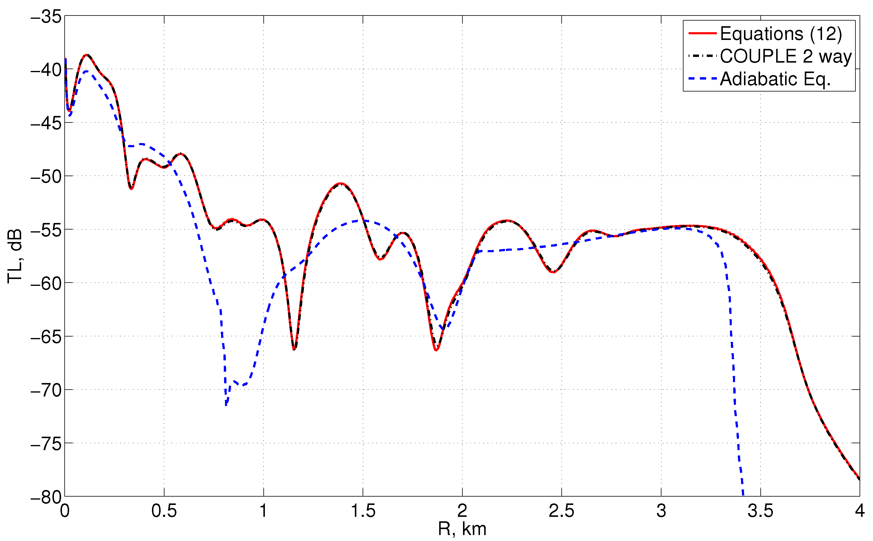
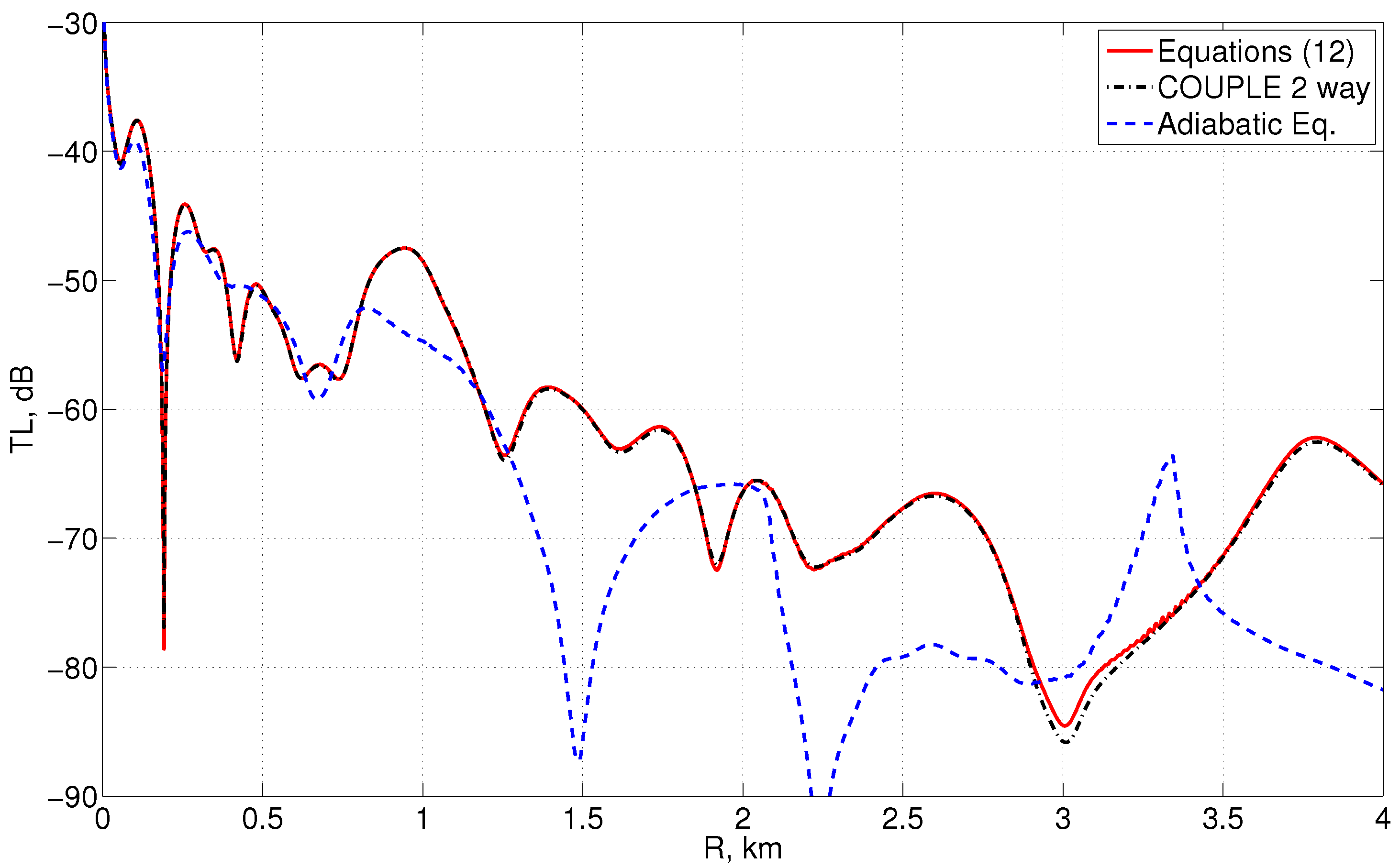
Figure 1 illustrates the dependence of the transmission loss on r for the receiver depth of 30 m obtained by solving coupled equations for mode amplitudes (23) and its adiabatic counterpart. With use a numerical solution obtained by using widely accepted COUPLE code [24] as a reference. It can be seen from Figure 1 that coupled mode solution exhibits excellent agreement with the field computed by COUPLE. By contrast, the adiabatic solution substantially differs from them. Indeed, it is known that in the upslope propagation scenario the waterborne modes excited by the source undergo cut-off one by one, until only bottom modes are left. Note that root mean square difference between the two coupled mode solution and the solution by couple in this case is about 0.15 dB. Similar results can be seen for the receiver depth of 150 m (usually these two depth are used in validation of various sound propagation models). The transmission loss curves are shown for this case in Figure 2. The root mean square difference between the solution obtained by solving Equation (23) and by COUPLE code in this case is about 0.4 dB.

It is no wonder that coupled mode models discussed here allow to obtain highly accurate solutions for the propagation scenarios with strong mode coupling by solving the equations for mode amplitudes on a relative coarse grid with the meshsize of about $\lambda /2$. Indeed, as it was shown above, we actually deal with a WKBJ-type approximation where the principal oscillation is cancelled (see Equation (10)), and the new unknown functions $B_j\left(r\right)$ are actually smooth envelopes for mode amplitudes.

7. Conclusions

In this study we present two different rigorous derivations of one-way coupled equations for mode amplitudes in the sea. Although similar equations have already appeared in the literature [2,12], the derivations above are, in our opinion, somewhat more clear, and within the asymptotic framework of this study the role of each of the involved approximations is very clearly seen. By contrast to other known equations for mode amplitudes (see, e.g., [6,22]), the ones presented here are obtained by a WKBJ-type asymptotic methods, and, consequently, admit relatively large steps in range when solved numerically. In this respect, the presented coupled equations are similar to parabolic equations theory, where the principal oscillation is also cancelled out. In fact, it can be shown that Equation (13) can be obtained from coupled mode parabolic equations by neglecting derivatives with respect to y (or to polar angle $\theta$ in the horizontal plane).

It is also shown that the derived coupled equations asymptotically preserve energy flux conservation property of the Helmholtz equation. We rigorously proved a theorem that guarantees energy flux conservation modulo high-order infinitesimal quantities. These quantities are small as long as the assumptions under which the equations are derived hold true.

The test calculations were done for the penetrable wedge benchmark scenario and proved excellent agreement of the field obtained by solving mode coupling equations presented in this work with the solution of the Helmholtz Equation (1) computed by the COUPLE program [24].

Our study also highlights the multiscale nature of the modal representation of acoustic field. In the framework of the normal mode theory its spatial variations involve three different scales, the slowest of which is described by a stretched range coordinate R and corresponds to the envelope that modulates the fastest spatial variations associated with modal phases that actually work as carrier waves. The variations in depth z described by the modes are of some intermediate scale. This insight can be fully exploited when constructing mode parabolic approximations for solving 3D sound propagation problems. On the other hand, this somehow reveals the physical nature of low- and mid-frequency acoustic fields in shallow water that has not been discussed in the literature until now.

References

1. Jensen, F.B.; Kuperman, W.A.; Porter, M.B.; Schmidt, H. Computational Ocean Acoustics; Springer: Berlin/Heidelberg, Germany, 2011. [Google Scholar]
2. Katsnelson, B.; Petnikov, V.; Lynch, J. Fundamentals of Shallow Water Acoustics; Springer: Berlin/Heidelberg, Germany, 2012. [Google Scholar]
3. Luo, W.; Zhang, R.; Schmidt, H. An efficient and numerically stable coupled-mode solution for range-dependent propagation. J. Comput. Acoust. 2012, 20, 1250008. [Google Scholar] [CrossRef]
4. Fawcett, J.A. A derivation of the differential equations of coupled-mode propagation. J. Acoust. Soc. Am. 1992, 92, 290–295. [Google Scholar] [CrossRef]
5. Porter, M.B.; Reiss, E.L. A numerical method for bottom interacting ocean acoustic normal modes. J. Acoust. Soc. Am. 1985, 77, 1760–1767. [Google Scholar] [CrossRef]
6. Godin, O.A. A note on differential equations of coupled-mode propagation in fluids. J. Acoust. Soc. Am. 1998, 103, 159–168. [Google Scholar] [CrossRef]
7. Godin, O.A. Coupled-mode sound propagation in a range-dependent, moving fluid. J. Acoust. Soc. Am. 2002, 111, 1984–1995. [Google Scholar] [CrossRef] [PubMed]
8. Stotts, S.A.; Koch, R.A. A two-way coupled mode formalism that satisfies energy conservation for impedance boundaries in underwater acoustics. J. Acoust. Soc. Am. 2015, 138, 3383–3396. [Google Scholar] [CrossRef] [PubMed]
9. Nayfeh, A.H. Perturbation Methods; John Wiley and Sons: New York, NY, USA, 1973; p. 437. [Google Scholar]
10. Trofimov, M.Y.; Kozitskiy, S.; Zakharenko, A. A mode parabolic equation method in the case of the resonant mode interaction. Wave Motion 2015, 58, 42–52. [Google Scholar] [CrossRef]
11. Maslov, V.P.; Fedoriuk, M.V. Semi-Classical Approximation in Quantum Mechanics; Springer: Berlin/Heidelberg, Germany, 2001; Volume 7. [Google Scholar]
12. Petrov, P.S.; Kazak, M.S.; Petrova, T.N. A generalization of WKBJ method for solving a system describing propagation of coupled modes in underwater acoustics. Phys. Lett. A 2022, 450, 128383. [Google Scholar] [CrossRef]
13. Landau, L.D.; Lifshitz, E.M. Quantum Mechanics: Non-Relativistic Theory; Elsevier: Amsterdam, The Netherlands, 2013; Volume 3. [Google Scholar]
14. Kozitskiy, S. Coupled-Mode Parabolic Equations for the Modeling of Sound Propagation in a Shallow-Water Waveguide with Weak Elastic Bottom. J. Mar. Sci. Eng. 2022, 10, 1355. [Google Scholar] [CrossRef]
15. Petrov, P.; Makarov, D.; Ehrhardt, M. Wide-angle parabolic approximations for the nonlinear Helmholtz equation in the Kerr media. Europhys. Lett. 2016, 116, 24004. [Google Scholar] [CrossRef]
16. Petrov, P.S.; Ehrhardt, M.; Tyshchenko, A.G.; Petrov, P.N. Wide-angle mode parabolic equations for the modelling of horizontal refraction in underwater acoustics and their numerical solution on unbounded domains. J. Sound Vib. 2020, 484, 115526. [Google Scholar] [CrossRef]
17. Liu, L.; Qin, Y.; Xu, Y.; Zhao, Y. The uniqueness and existence of solutions for the 3-D Helmholtz equation in a stratified medium with unbounded perturbation. Math. Methods Appl. Sci. 2013, 36, 2033–2047. [Google Scholar] [CrossRef]
18. Sveshnikov, A. The radiation principle. Dokl. Akad. Nauk SSSR 1950, 73, 917–920. [Google Scholar]
19. Naimark, M.A. Linear Differential Operators. Elementary Theory of Linear Differential Operators: With Additional Material by the Author, Part I; Frederick Ungar Publishing Company: New York, NY, USA, 1967; p. 144. [Google Scholar]
20. Petrov, P.; Trofimov, M.Y.; Zakharenko, A. Modal perturbation theory in the case of bathymetry variations in shallow-water acoustics. Russ. J. Math. Phys. 2021, 28, 257–262. [Google Scholar] [CrossRef]
21. Zakharenko, A.; Petrov, P. Perturbations of Modal Attenuation Coefficients and Group Velocities due to Depth Variations along a Shallow-Water Acoustic Track. Acoust. Phys. 2022, 68, 575–581. [Google Scholar] [CrossRef]
22. Brekhovskikh, L.M.; Godin, O.A. Acoustics of Layered Media I: Plane and Quasi-Plane Waves; Springer: Berlin/Heidelberg, Germany, 2012; Volume 5. [Google Scholar]
23. Landau, L.D.; Lifshits, E.M. Fluid Mechanics, Course of Theoretical Physics; Pergamon Press: Oxford, UK, 1999; Volume 6, p. 539. [Google Scholar]
24. Evans, R.B. COUPLE, Documentation. 2007. Available online: https://oalib-acoustics.org/website_resources/Modes/couple/COUPLE07.tx&quot (accessed on 28 March 2023).
Figure 1. Transmission loss for the propagation along the bottom slope as a function of distance r from the source in ASA wedge benchmark computed by solving equations for mode amplitudes (23). The reference solution is obtained by the COUPLE program [24]. Adiabatic solution is shown for comparison. The source is deployed at the depth of 100 m, and the depth of the receiver is 30 m.
Jmse 11 00797 g001
Figure 2. Transmission loss for the propagation along the bottom slope as a function of distance r from the source in ASA wedge benchmark computed by solving equations for mode amplitudes (23). The reference solution is obtained by the COUPLE program [24]. Adiabatic solution is shown for comparison. The source is deployed at the depth of 100 m, and the depth of the receiver is 150 m.
Jmse 11 00797 g002
Disclaimer/Publisher’s Note: The statements, opinions and data contained in all publications are solely those of the individual author(s) and contributor(s) and not of MDPI and/or the editor(s). MDPI and/or the editor(s) disclaim responsibility for any injury to people or property resulting from any ideas, methods, instructions or products referred to in the content.