Article

Random Matrix Theory for Sound Propagation in a Shallow-Water Acoustic Waveguide with Sea Bottom Roughness

by
Denis V. Makarov
1,*,
Pavel S. Petrov
1,2 and
Michael Yu. Uleysky
1
1
V.I. Il’ichev Pacific Oceanological Institute of the Far-East Branch of the Russian Academy of Sciences, 690041 Vladivostok, Russia
2
Fakultät IV–Mathematik und Naturwissenschaften, Bergische Universität Wuppertal, Gaußstraße 20, 42119 Wuppertal, Germany
*
Author to whom correspondence should be addressed.
J. Mar. Sci. Eng. 2023, 11(10), 1987; https://doi.org/10.3390/jmse11101987
Submission received: 31 August 2023 / Revised: 2 October 2023 / Accepted: 12 October 2023 / Published: 14 October 2023
(This article belongs to the Special Issue Sound Scattering in the Ocean)

Abstract

:
The problem of sound propagation in a shallow sea with a rough sea bottom is considered. A random matrix approach for studying sound scattering by the water–bottom interface inhomogeneities is developed. This approach is based on the construction of a statistical ensemble of the propagator matrices that describe the evolution of the wavefield in the basis of normal modes. A formula for the coupling term corresponding to inter-mode transitions due to scattering by the sea bottom is derived. The Weisskopf–Wigner approximation is utilized for the coupling between waterborne and sediment modes. A model of a waveguide with the bottom roughness described by the stochastic Ornstein–Uhlenbeck process is considered as an example. Range dependencies of mode energies, modal cross coherences and scintillation indices are computed using Monte Carlo simulations. It is shown that decreasing the roughness correlation length enhances mode coupling and facilitates sound scattering.

1. Introduction

Sound scattering by random inhomogeneities of the marine environment is one of the fundamental problems in ocean acoustics. Usually, multiple scattering of acoustic signals causes phase and amplitude fluctuations and complicates interference pattern and dispersion characteristics [1]. This process acts as an obstacle preventing the application of acoustic methods to solving various practical problems in marine science, e.g., underwater communication and navigation [2,3,4,5], or hydroacoustical tomography [6,7,8,9,10].
The stochastic nature of inhomogeneities anticipates the usage of statistical methods for their description. Typically, longitudinal inhomogeneities of the marine environment are relatively weak and can be fairly described as perturbations superimposed onto a range-independent waveguide, in which the acoustic field is conveniently described in terms of normal modes. This explains why mode-based approaches taking the effect of scattering into account via the mode coupling are widely used in underwater acoustics community [11].
One of the most popular approaches is the derivation of coupled kinetic equations for ensemble-averaged modal intensities. It was originally proposed in the seminal work of Tappert of Dozier [12], and further developed in a series of papers [13,14,15,16]. The ray-based theory of mode coupling was developed by Virovlyansky [17]. In the present paper, we consider another promising approach based on the construction of a wavefield propagator based on the random matrix theory [18,19]. By definition, a propagator is an operator that governs wavefield evolution in the course of its propagation along the waveguide [20]. The matrix representation of the propagator can be obtained using the basis of normal modes, and the matrix elements are complex-valued random amplitudes of intermode transitions (the propagator matrices considered here are not to be confused with the ones emerging in the vector–matrix formalism [21] for the representation of the solutions for wave equations). The main advantage of this approach is the possibility to take into account interference effects within a full-wave picture. We conducted early studies of a wavefield propagator for idealized range-periodic waveguides in the context of the wave chaos problem [22,23,24]. The propagator properties for waveguides with random inhomogeneities caused by linear internal waves were considered in [25,26,27]. The case of nonlinear internal waves was considered in [28,29,30]. In [31], this approach was generalized onto the case of waveguides with adiabatic longitudinal variations. The propagator taking into account temporal variability of the medium was considered in [5].
In the majority of works concerning the wavefield propagators for randomly inhomogeneous waveguides, deep-water propagation scenarios with volumetric inhomogeneities were investigated. At the same time, the propagators describing sound scattering on random sea bottom roughnesshave not been thoroughly studied until now. Indeed, scattering from rough surfaces is a fairly extensive field of wave physics (see, for example, a brief review [32], or another paper from the present special issue [33]). However, multiple scattering from roughness in waveguides has some specific features and still is a predominantly open problem. Sound scattering of this kind has a lot in common with the general problem of wave transport in disordered quantum mesoscopic waveguides [34,35], and some of the ideas of the matrix propagator theory are drawn from there (this issue is discussed in [18]). In fact, the problem of scattering from bottom roughness is of great importance for shallow-sea acoustics, mainly due to the fact that in real-world applications, the information on the bathymetry is often insufficiently accurate. To our knowledge, the first paper studying acoustic mode interaction in a waveguide with range-dependent bathymetry is [36]. A kind of a wavefield propagator for a shallow sea was studied in [37], where a waveguide with randomly perturbed interfaces was considered, and the staircase approximation was used for the interface representation. In addition, we can mention the paper [38] devoted to the effect of scattering from the rough sea bottom on modal energies, and the paper [39] with the application of the cross-section method to a waveguide with random bathymetry.
In the present paper, we develop a theoretical approach that goes beyond the staircase approximation used in [37] and allows one to take into account the actual form of the sea bottom roughness. In addition, the particular case of the roughness described by the stochastic Ornstein–Uhlenbeck process is considered.
The paper is organized as follows. In the next section, we represent the general theory of the non-unitary matrix propagator for a shallow sea. Section 3 is devoted to the construction of the matrix propagator in the presence of bottom roughness. The particular case of the roughness described by the Ornstein–Uhlenbeck process is analyzed in Section 4. Section 5 presents the result of the numerical simulation of a model waveguide with a near-bottom sound channel. In the Discussion setion, we summarize the main results and outline the ways of further development of the approach.

2. General Theory

We start with the Helmholtz equation in cylindrical coordinates r , θ , z . Under the assumption that azimuthal coupling is weak (i.e., the derivative with respect to θ can be neglected), it can be written as
2 P r 2 + 1 r P r + ρ z 1 ρ P z + k 0 2 n 2 P = 0 ,
where r is the range, z is the depth, P ( r , z ) is the acoustic pressure, ρ is the density, k 0 = 2 π f / c 0 is a reference wavenumber, c 0 is a reference sound speed, and n ( r , z ) is the refractive index. Invoking the far-field approximation and neglecting back-scattering, we can transform Equation (1) to a one-way equation for the wavefield envelope function Ψ = P k 0 r exp ( i k 0 r ) :
Ψ r = i k 0 Q ^ 1 Ψ ,
where the prefactor k 0 r takes into account cylindrical sound spreading, and the operator Q ^ is given by the expression [40]
Q ^ = n 2 + 1 k 0 2 ρ z 1 ρ z .
The solution of Equation (2) can be formally written in terms of the propagator G ^ defined as
Ψ ( r , z ) = G ^ ( r , r 0 ) Ψ ( r 0 , z ) .
In order to facilitate the calculation of G ^ , it is reasonable to use the basis of normal modes, i.e., solutions of the Sturm–Liouville problem [40]
k 0 2 Q ^ 2 Ψ m = k r m 2 Ψ m ,
with properly imposed boundary and interface conditions [40]. A wavefield can be represented as an expansion over normal modes:
Ψ ( r , z ) = m a m ( r ) Ψ m ( z ) .
The amplitude of the m-th mode is determined as
a m ( r ) = z = 0 h Ψ m * ( r , z ) Ψ ( r , z ) ρ ( z ) d z .
Hereafter, we consider the case of weak range dependence, assuming that the operator Q ^ can be expressed as a sum of the range-independent part Q ^ 0 and a small perturbation V ^ , i.e.,
Ψ r = i k 0 Q ^ 0 + V ^ ( r ) 1 Ψ .
In the rest of this study we assume that modes in the Sturm–Liouville problem (5) are computed for Q ^ = Q ^ 0 , i.e., for the reference range-independent waveguide.
Substituting the ansatz (6) into Equation (8), and taking into account that Ψ m satisfies (5) for Q ^ = Q ^ 0 , we obtain a system of coupled equations for the modal amplitudes a m ( r ) :
d a m d r = i ( k r m k 0 ) a m + i k 0 n V m n ( r ) a n ,
where
V m n ( r ) = 1 ρ ( z ) Ψ m * ( z ) V ^ ( r ) Ψ n ( z ) d z
are the matrix elements of the operator V ^ . Equation (9) is similar to the perturbation theory for the Schrödinger equation in the way it is derived in [41], where the wave function of the perturbed (time-dependent) quantum system is represented in the form of expansion over the eigenstates of its counterpart with the time-independent Hamiltonian. Other approaches to the derivation of the mode coupling equations can be found in [11,40,42,43,44].
Using the substitution
b m ( r ) = a m ( r ) e i ( k r m k 0 ) r ,
we can transform Equation (9) to the following form:
d b m d r = i k 0 n V m n e i ( k r n k r m ) r b n .
It is formally equivalent to a Volterra-type integral equation
b m ( r ) = b m ( r = r 0 ) + i k 0 n r = r 0 r V m n e i ( k r n k r m ) r b n ( r ) d r .
The respective expression for mode amplitudes a m reads as
a m = e i ( k r m k 0 ) r a m ( r = 0 ) + i k 0 n r = 0 r V m n ( r ) e i ( k r n k r m ) r a n ( r ) d r .
Basically, there are two kinds of modes in a shallow-water waveguide: waterborne modes with weak attenuation, and modes predominantly propagating inside the bottom sediment layer and experiencing strong losses. In practice, the latter ones are poorly known (due to the lack of data about precise bottom structure), and it is reasonable to exploit the fact that their contribution to the field is relatively small. This can be performed in the spirit of the Weisskopf–Wigner approach that is well known in the theory of open quantum systems [45]. Without loss of generality, we can assume that waterborne modes correspond to m M , and modes with m > M have maxima in the bottom.
The expansion (6) can be rewritten as
Ψ ( r , z ) = m = 1 M b m ( r ) e i ( k r m k 0 ) r Ψ m ( z ) + m = M + 1 M max b m ( r ) e i ( k r m k 0 ) r Ψ m ( z ) ,
where M max is the total number of discrete-spectrum modes taken into account. Separating the contributions of water and sedimental modes in (12), we have
d b m d r = i k 0 n = 1 M V m n ( r ) e i ( k r n k r m ) r b n + i k 0 n = M + 1 M max V m n ( r ) e i ( k r n k r m ) r b n .
Waterborne and sedimental modes overlap weakly; therefore, transitions between them can be considered a second-order effect. Except for very low frequencies, the sedimental modes have very strong attenuation; therefore, we can neglect the scattering of acoustic energy from sedimental to water modes. Since it is natural to assume that only the water modes are excited at r = r 0 , it means that solutions for the sedimental modes can be written as
b n ( r ) = i k 0 n = 1 M max r = r 0 r V n n ( r ) e i ( k r n k r n ) r b n ( r ) d r , n > M .
Substituting (17) into (16), we obtain equations for modes with m M
d b m d r = i k 0 n = 1 M V m n ( r ) e i ( k r n k r m ) r b n       k 0 2 n = M + 1 M max n = 1 M max r = r 0 r V m n ( r ) V n n ( r ) e i ( k r n k r m ) r + i ( k r n k r n ) r b n ( r ) d r .
If r is sufficiently large, only the terms with n = m efficiently contribute to this double sum, and we rewrite the latter equality as
d b m d r = i k 0 n = 1 M V m n ( r ) e i ( k r n k r m ) r b n       k 0 2 n = M + 1 M max r = r 0 r V m n ( r ) V n m ( r ) e ( α m α n ) ( r r ) e i ( k n k m ) ( r r ) b m ( r ) d r ,
where k m = k r m , α m = k r m . The second term describes the mode attenuation caused by coupling to sedimental modes. Here, we do not imply any symmetries for the perturbation matrix, assuming that in general V m n V n m .
Below, we consider only the case of an operator V ^ describing some stationary random process. It means that the corresponding matrix elements V m n ( r ) are stationary random functions as well, and Equation (19) is stochastic with non-Markovian kernels [15,46]. The presence of V m n within the kernels anticipates fluctuations of attenuation. However, as long as perturbation is assumed to be weak, matrix elements V m n are small. Therefore, we can ignore fluctuations of attenuation and replace the product V m n V n m by its statistical average. Also, we can take into account that sedimental modes have much higher damping rates α m . This implies that the function
C m n ( r , r ) = V m n ( r ) V n m ( r ) e ( α m α n ) ( r r ) , n > M ,
rapidly decays with increasing | r r | . This allows us to invoke the Markov approximation and ignore range non-locality. Thus, we obtain
d b m d r = i k 0 n = 1 M V m n ( r ) e i ( k r n k r m ) r b n Γ m b m .
Here the damping coefficients Γ m are evaluated by means of the Wiener–Khintchin theorem,
Γ m = k 0 2 n = M + 1 M max C ˜ m n ( Δ k m n ) , Δ k m n = k m k n ,
where C ˜ m n ( k ) is Fourier-transformed C m n ( r ) . Invoking the perturbation theory for Equation (21) and taking into account (11), we obtain the first-order approximation for the waterborne modes in the following form:
a m ( r ) = e i k m r γ m r a m ( r = 0 ) + i k 0 n = 1 M r = 0 r V m n ( r ) e i ( k r n k r m ) r a n ( r ) d r ,
where γ m = α m + Γ m . This equation can be rewritten in the matrix form as
G ( r , r 0 ) = Λ ( I + i A ) ,
where I is the identity matrix, and Λ is a diagonal matrix corresponding to the unperturbed propagator
Λ m n ( r , r 0 ) δ m n e i ( k r m k 0 ) ( r r 0 ) ,
and A is the perturbation matrix with elements
A m n ( r , r 0 ) = k 0 r = 0 r V m n ( r ) e i ( k r n k r m ) r d r .
Note that within this study bold letters denote matrices, e.g., A , while their respective elements are written as A m n .
The key idea of the approach based on random matrix theory is to represent matrix elements A m n as random Gaussian variables whose variance is determined by variance of the integral (26). This approach is well developed in the case of deep-water acoustic waveguides with volume inhomogeneities, when the propagator is nearly unitary [18,19,27,31].
The validity of the first-order perturbation theory demands the propagator step to be sufficiently small. In order to perform long-range propagation modeling, we can partition the waveguide into short segments of length Δ r , and represent the resulting propagator as a product
G ^ ( r F , r 0 ) = G ^ ( r F , r F Δ r ) G ^ ( r F Δ r , r F 2 Δ r ) . . . G ^ ( r 0 + Δ r , r 0 ) ,
or, in the matrix representation,
G ( r F , r 0 ) = G ( r F , r F Δ r ) G ( r F Δ r , r F 2 Δ r ) . . . G ( r 0 + Δ r , r 0 ) ,
Now the segment propagators can be obtained from Equation (24).

3. Random Sea Bottom Roughness

Let us now consider the case where the water depth randomly fluctuates with the range r, i.e.,
h ( r ) = h 0 + δ h ( r ) ,
where δ h ( r ) is some random function to be specified later. To derive the expression for the perturbation operator V ^ , it is convenient to introduce the rescaled depth variable
Z = h 0 h ( r ) z = 1 1 + η z ,
where
η δ h h 0 .
Similar transformations of variables are often used in quantum–mechanical problems with moving boundaries [47,48,49]. We assume that variations of the water depth are weak, i.e., that η 1 . Transformation of the depth variable (30) leads to the transformation of derivatives in (2) and (3):
r r + Z ( h / r ) h Z ,
z 1 ( 1 + η ) Z .
Substituting (32) and (33) into (2) and (3), we obtain
Ψ r = Z h d h d r Ψ Z + i k 0 n 2 ( r , Z ) + ρ ( r , Z ) k 0 2 ( 1 + η ) 2 Z 1 ρ ( r , Z ) Z 1 Ψ .
As long as η is small compared to 1, we can separate the range-independent and range-dependent parts of n 2 ( r , Z ) and ρ ( r , Z ) using the Taylor expansion. Leaving only the zero-order and first-order terms, we have
n 2 ( r , Z ) = n 0 2 ( Z ) + 2 n 0 ( Z ) n 0 Z Z η ( r ) ,
ρ ( r , Z ) = ρ 0 ( Z ) + ρ Z Z η ( r ) ,
where
n 0 ( Z ) n ( Z ) | η = 0 ,
ρ 0 ( Z ) ρ ( Z ) | η = 0 .
For the sake of simplicity, we neglect the terms involving ρ / Z . Also, we can take into account that
1 h d h d r d η d r , 1 ( 1 + η ) 2 1 2 η .
Now Equation (34) can be rewritten as
Ψ r = i d η d r D ^ a Ψ + i k 0 n 0 2 ( r , Z ) + ρ 0 ( Z ) k 0 2 Z 1 ρ 0 ( Z ) Z + 2 η ( r ) D ^ b 1 Ψ ,
where differential operators D ^ a and D ^ b are given by expressions
D ^ a = i Z Z ,
D ^ b = n 0 ( Z ) n 0 Z Z ρ 0 ( Z ) k 0 2 Z 1 ρ 0 ( Z ) Z .
In order to find out the resulting perturbation operator V ^ (see (8)), we have to extract the perturbation term containing η ( r ) from the square-root operator. This problem can be solved by means of the Taylor approximation (which is widely used in similar studies, see, for example, [50]):
Q ^ Q ^ 0 + 1 + 2 η ( r ) D ^ b 1 Q ^ 0 + η ( r ) D ^ b .
After such transformation, the perturbation operator reads as
V ^ ( r ) = 1 k 0 d η ( r ) d r D ^ a + η ( r ) D ^ b ,
Matrix elements of the operator V ^ are expressed as
V m n = 1 k 0 d η ( r ) d r D a , m n + η ( r ) D b , m n ,
where
D a , m n = Ψ m * ( Z ) D ^ a Ψ n ( Z ) ρ 0 ( Z ) d Z ,
D b , m n = Ψ m * ( Z ) D ^ b Ψ n ( Z ) ρ 0 ( Z ) d Z ,
and normal modes Ψ n ( z ) correspond to the unperturbed problem with V ^ = 0 . Elements of the perturbation matrix A are given by the formula
A m n ( Δ r ) = k 0 υ a , m n D a , m n + υ b , m n D b , m n ,
where
υ a , m n = 1 k 0 r = 0 Δ r d η d r ( r ) e i ( k r n k r m ) r d r ,
υ b , m n = r = 0 Δ r η ( r ) e i ( k r n k r m ) r d r .
Here, υ a , m n and υ b , m n are stochastic integrals which depend on statistical properties of η ( r ) . The presence of nonzero imaginary parts of wavenumbers k r n destroys symmetries of the matrix A . However, the attenuation of water modes is usually weak and obeys inequality k r n Δ r 1 . Therefore, we can neglect the impact of imaginary parts in Equations (47) and (48) and assume k r n k n . Then, Equations (47) and (48) read as
υ a , m n = 1 k 0 r = 0 Δ r d η d r ( r ) e i ( k n k m ) r d r ,
υ b , m n = r = 0 Δ r η ( r ) e i ( k n k m ) r d r .

4. Ornstein–Uhlenbeck Sea Bottom Roughness

In this section, we consider the sea bottom roughness described by the formula
η ( r ) = σ η η ¯ ( r ) ,
where η ¯ ( r ) is the normalized stochastic Ornstein–Uhlenbeck process being the solution of the Langevin equation
d η ¯ d r = η ¯ r c + 2 r c ξ .
In this formula, r c is the roughness correlation length, and ξ is Gaussian white noise,
ξ = 0 , ξ ( r ) ξ ( r ) = δ ( r r ) ,
δ ( r ) is the delta function, and angular brackets denote ensemble averaging. Roughness autocorrelation function is given by [51]
C η ( s ) = η ( r ) η ( r s ) = σ η 2 e | s | r c .
Taking into account (52), we find
υ a , m n = υ b , m n k 0 r c + σ η k 0 2 r c ξ a , m n ,
where ξ a , m n is a Gaussian complex random variable with zero mean and unit variance. These Gaussian variables obey the relation
ξ a , m n = ξ a , n m * .
In order to find the corresponding expression for υ b , m n , we can use spectral representation of the Ornstein–Uhlenbeck process:
η = d k S ( k ) e i ( k r + ϕ ( k ) ) ,
where ϕ ( k ) is a random phase function obeying
π ϕ π , ϕ ( k ) = ϕ ( k ) , ϕ ( k ) ϕ ( k ± k ) = 0 ,
and S ( k ) is the power spectrum of η ( r ) given by the formula
S ( k ) = C ( s ) e i k s d s = σ η 2 r c π ( 1 + k 2 r c 2 ) .
Substituting (57) into (48), we obtain
υ b , m n = σ m n ξ b , m n ,
where ξ a , m n is another Gaussian random variable with zero mean and unit variance, also obeying
ξ b , m n = ξ b , n m * .
and the corresponding variance is determined via the formula
σ m n 2 = d k S ( k ) sin c 2 ( k + k n k m ) Δ r 2 .
The resulting expression for perturbation matrix elements can be written as
A m n = k 0 D a , m n 2 Δ r r c ξ a , m n + W m n ξ b , m n ,
where
W m n = D b , m n υ a , m n k 0 r c .
In order to evaluate the coefficients of damping caused by coupling to sedimental modes, one has to compute the correlator C m n ( r , r ) (20). Let us denote η = d η / d r and recall that
ξ ( r ) η ( r s ) = 0 .
Then, according to (52), we have
η ( r ) η ( r s ) = 1 r c C η ( s ) , η ( r ) η ( r s ) = C η ( s ) r c 2 + 2 r c δ ( s ) ,
where δ ( s ) is the delta function. The correlator can therefore be written as
C m n ( r , r ) = σ η 2 W m n 2 exp 1 r c + α n α m | r r | + 2 D a , m n k 0 2 r c δ ( r r ) .
Applying the Wiener–Khintchin theorem, we find that
C ˜ ( k ) = 2 D a , m n 2 k 0 2 r c + σ η 2 W m n 2 π γ c ( 1 + k 2 r c 2 ) ,
where
γ c = 1 r c + α n α m .

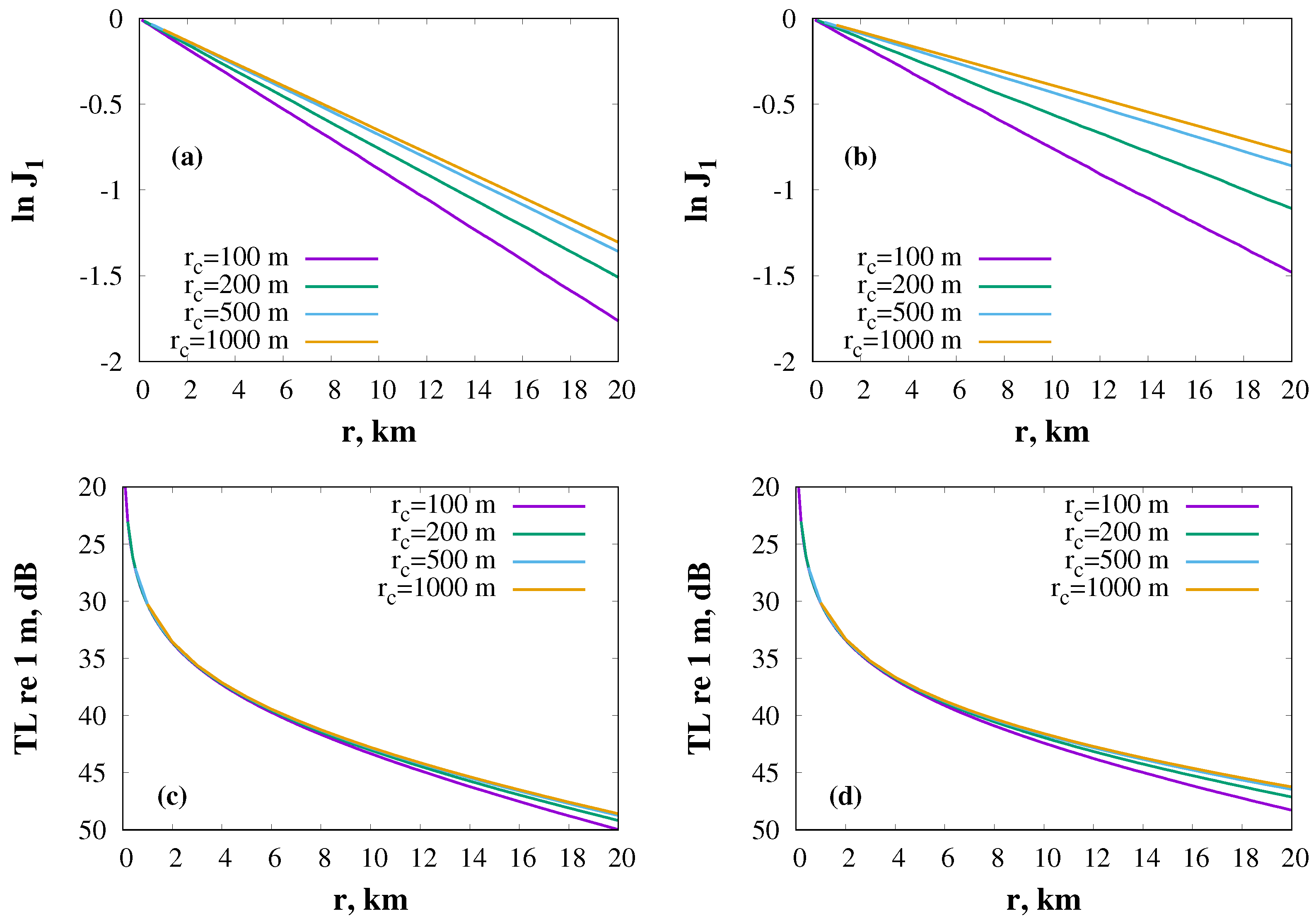
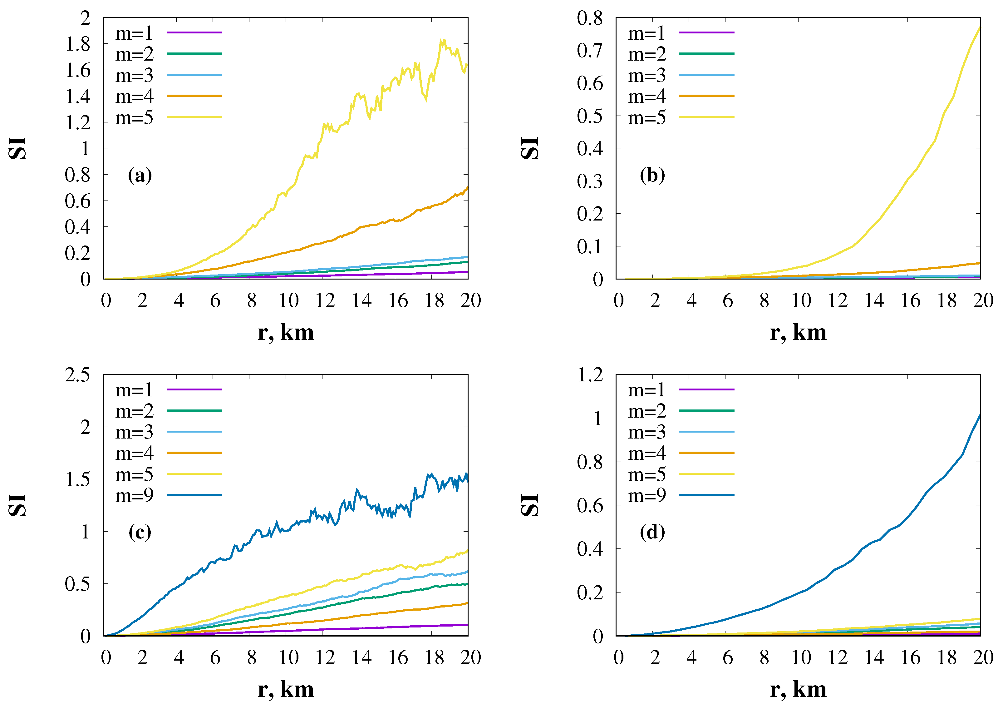
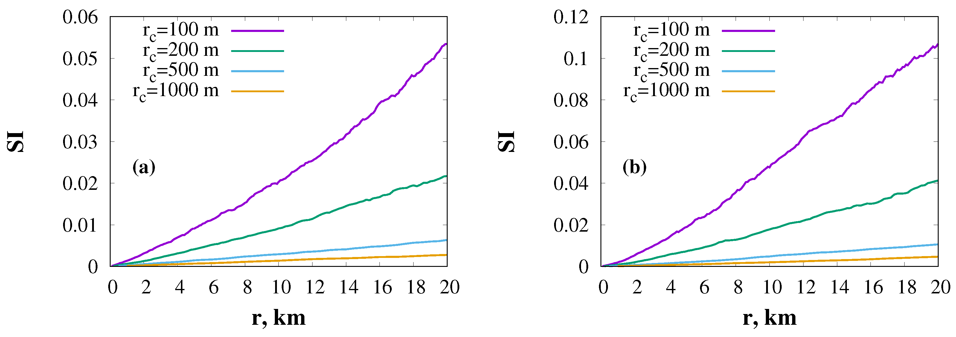
5. Numerical Simulation

For the numerical simulation, we use a model of a shallow-water waveguide with the sound–speed profile described by the formula [52,53,54]
c ( z ) = c 0 Δ c 2 1 + tanh z z c Δ z , 0 z < h , c b , h z L ,
where c 0 = 1500 m/s is the sound speed at the ocean surface, Δ c = 25 m/s, z c = 50 m, Δ z = 10 m, c b = 1600 m/s, and L = 300 m. The interface at the depth z = h = 100 m separates the water water column and sediment layer. The sound speed profile in the water is presented in Figure 1.
The magnitude of the bottom roughness is σ η = 0.01 ; this corresponds to the r.m.s. displacement of 1 m. The correlation length of roughness r c is varied from 100 to 1000 m. The sediment attenuation coefficient is taken to be 0.5 dB per wavelength.
Calculation of the propagator described above is based on the mode perturbation theory that provides accurate prediction only for relatively low signal frequencies. We carried out the statistical modeling of propagator matrices for two values of frequency, namely 100 and 200 Hz. It was found that the number of waterborne modes in the considered model of a waveguide is related to the acoustic frequency via the formula f 20 M . That is, we have 5 waterborne modes for 100 Hz, and 10 waterborne modes for 200 Hz. The propagator step Δ r is taken to be equal to the correlation length of the roughness Δ r = r c . This ensures the applicability of the perturbation theory to the evaluation of the matrix elements of the propagator, and, on the other hand, meets the condition of statistical independence of the propagators for neighboring waveguide segments. This condition allows us to neglect the correlations between the segment propagators. For each set of the parameters, a statistical analysis is carried out using 1000 realizations of propagator matrices.
Firsly, let us examine range variations of modal energies. In the case of a single-mode source, normalized mean energies are determined by the formula
J m ( r ) = | a m ( r ) | 2 | a m ( r = 0 ) | 2 = | G m m ( r , 0 ) | 2 .
The angular brackets in this formula denote averaging over the ensemble of roughness realizations. Decreasing the roughness correlation length enhances the impact of scattering and transitions of mode energy to higher-order modes, exhibiting faster attenuation by the bottom. Therefore, in this case, the scattering increases energy losses. It is confirmed by the data presented in Figure 2 and Figure 3. Notably, in the case of the acoustic frequency of 100 Hz, the decay is exponential (this is revealed by the linear decreasing of the energy logarithm). In the case of f = 200 Hz, higher-order modes decay slower than the exponential rate due to the partial re-pumping from much more energetic lower-order modes. The presence of energy flux from lower to higher modes due to mode coupling is illustrated in Figure 3a,b, where the range dependence of the first mode energy is depicted. It is shown that decreasing r c , anticipating stronger coupling, leads to faster attenuation.
Decay of the first mode energy consists of two components: energy transfer to the sedimental modes with high loss, and energy transfer to the waterborne modes with relatively low loss. To eliminate the contribution of the latter component, we can estimate the roughness-induced enhancement of losses. In particular, we can consider the depth-integrated transmission loss for a wavefield created by a single-mode source. Using the propagator, it can be calculated using the formula
TL ( n , r ) = 10 log 10 r ref r m | G m n ( r , 0 ) | 2 ,
where r ref = 1 m. The corresponding data for n = 1 are presented in Figure 3c,d. It turns out that the coupling of the first mode to lossy sedimental modes is fairly weak; therefore, the bottom roughness weakly influences transmission loss.
Another characteristics that can be used for the description of mode coupling is modal cross-coherence defined as
J m n ( r ) = | a m ( r ) a n * ( r ) | | a m ( r ) | 2 | a n ( r ) | 2 ,
where range dependencies of modal amplitudes are calculated for the initial conditions of the following form:
a j = 1 2 , j = m , n , 0 , j m , n .
We focus our attention on the cross-coherence of the first mode with other waterborne modes. Data for frequency of 100 Hz are presented in Figure 4. The data suggest that the first three modes maintain a high degree of coherence throughout the entire distance under consideration. On the other hand, the fifth mode experiencing the strongest scattering among the waterborne modes undergoes the fastest decoherence.
In the case of f = 200 Hz (see Figure 5), we also consider the first five modes. However, as the frequency is increased, these modes correspond to flatter rays [55] that are less in contact with the sea bottom roughness. Therefore, they expose much weaker scattering: considerable decoherence is observed only in the case of short-range roughness. In the cases of r c = 500 and 1000 m, the cross-coherence decay is very weak.
Fluctuations of modal amplitudes can be estimated by means of the corresponding scintillation index defined as
SI ( m , r ) = | G m m ( r , 0 ) | 2 | G m m ( r , 0 ) 2 1 .
The data presented in Figure 6 demonstrates the growth of fluctuations as the unperturbed (i.e., calculated in the unperturbed waveguide without roughness) modal attenuation rate increases. However, with a distance of 20 km, only the highest waterborne modes manage to achieve statistical saturation with SI 1 [56]. Moreover, in the case of f = 100 Hz (see Figure 4a,b), even the highest five modes do not achieve plateau, despite the high values of the scintillation index. It means that saturation for low-frequency propagation should occur at longer distances. According to Figure 7, the first mode exposes very weak fluctuations for all values of the roughness correlation length, anticipating nearly adiabatic propagation. Comparing Figure 7a,b, a twofold increase in frequency leads to a twofold increase in the scintillation index, implying that the fluctuation strength is proportional to the frequency.

6. Discussion

In the present study, we outline a novel approach to the modeling of sound scattering by random sea bottom roughness. This approach is based on the construction of random propagator matrices. It is a very computationally efficient tool for wavefield modeling that has many other attractive features as well. In particular, the propagator takes into account almost all information about the acoustic properties of the waveguide segment under consideration. Therefore, it can provide comprehensive information about the scattering physics, including statistics of losses and fluctuations, and estimates of cross-modal coherence, as well as the behavior of many other wavefield parameters.
We derive explicit analytical expressions for the propagator matrix elements for roughness described by the stochastic Ornstein–Uhlenbeck process. It is very important from the viewpoint of practical implementation, as the Ornstein–Uhlenbeck process represents a typical example of roughness with exponentially decaying autocorrelation function that can be a good model of realistic water depth variations in a shallow sea. Statistical analysis of sound propagation in a shallow-sea with the Ornstein–Uhlenbeck bottom roughness shows that the low-order modes are weakly affected by the scattering and exhibit highly unsaturated statistics of fluctuations. Nevertheless, mode coupling due to scattering results in significant increasing of attenuation rates of the lowest-order modes. Decreasing the roughness correlation length leads to drastic enhancement of the scattering, especially for the highest waterborne modes. It is reflected as the fast decay of cross-mode coherence functions, as well as the sharp increase in the modal scintillation indices. Such enhancement of scattering was earlier reported in [39].
Further development of the propagator approach based on the random matrix theory, in our opinion, should involve generalization to 3D propagation scenarios [57,58,59]. This can be accomplished, for example, in the framework of pseudodifferential mode parabolic equations [60,61]. Indeed, the effect of the horizontal refraction on the field at a reception point can be very significant in a shallow sea. Some phenomena similar to the branching of light beams in optics can be expected in this case [62]. Another promising direction of generalization of the results presented here is the development of the random matrix theory for broadband signals that would accurately handle inter-frequency correlations. Finally, the results of the present work can be extended to the case of an elastic bottom by using the approach proposed in [63]. Arguably, bottom elasticity would not significantly change the results of the numerical experiments reported here, as one can expect its contribution to manifest primarily in somewhat greater attenuation coefficients of the bottom modes.

Author Contributions

Conceptualization, D.V.M. and P.S.P.; methodology and formal derivations, D.V.M. and M.Y.U.; software, D.V.M. and P.S.P.; numerical experiments, D.V.M.; writing—original draft preparation, D.V.M.; writing—review and editing, P.S.P. All authors have read and agreed to the published version of the manuscript.

Funding

The work of all authors at POI is within state assignment program No. 121021700341-2.

Institutional Review Board Statement

Not applicable.

Informed Consent Statement

Not applicable.

Data Availability Statement

Not applicable.

Conflicts of Interest

The authors declare no conflict of interest.

References

  1. Dashen, R.; Flatté, S.M.; Munk, W.H.; Watson, K.M.; Zachariasen, F. Sound Transmission through a Fluctuating Ocean; Cambridge University Press: Cambridge, UK, 2010; p. 320. [Google Scholar]
  2. Chitre, M.; Shahabudeen, S.; Stojanovic, M. Underwater Acoustic Communications and Networking: Recent Advances and Future Challenges. Mar. Technol. Soc. J. 2008, 42, 103–116. [Google Scholar] [CrossRef]
  3. Virovlyansky, A.L.; Kazarova, A.Y.; Lyubavin, L.Y. Focusing of sound pulses using the time reversal technique on 100-km paths in a deep sea. Acoust. Phys. 2012, 58, 678–686. [Google Scholar] [CrossRef]
  4. Morgunov, Y.N.; Golov, A.A.; Burenin, A.V.; Petrov, P.S. Studies of spatiotemporal structure of the acoustic field formed in deep water by a broadband pulsed signal source on the shelf of the Sea of Japan. Acoust. Phys. 2019, 65, 537–544. [Google Scholar] [CrossRef]
  5. Makarov, D.V.; Komissarov, A.A. Chaos and wavefront reversal for long-range sound propagation. Dokl. Earth Sci. 2022, 507, 1118–1123. [Google Scholar] [CrossRef]
  6. Tappert, F.D.; Tang, X. Ray chaos and eigenrays. J. Acoust. Soc. Am. 1996, 99, 185–195. [Google Scholar] [CrossRef]
  7. Worcester, P.F.; Cornuelle, B.D.; Dzieciuch, M.A.; Munk, W.H.; Howe, B.M.; Mercer, J.A.; Spindel, R.C.; Colosi, J.A.; Metzger, K.; Birdsall, T.G.; et al. A test of basin-scale acoustic thermometry using a large-aperture vertical array at 3250-km range in the eastern North Pacific Ocean. J. Acoust. Soc. Am. 1999, 105, 3185–3201. [Google Scholar] [CrossRef]
  8. Colosi, J.A.; Scheer, E.K.; Flatté, S.M.; Cornuelle, B.D.; Dzieciuch, M.A.; Munk, W.H.; Worcester, P.F.; Howe, B.M.; Mercer, J.A.; Spindel, R.C.; et al. Comparisons of measured and predicted acoustic fluctuations for a 3250-km propagation experiment in the eastern North Pacific Ocean. J. Acoust. Soc. Am. 1999, 105, 3202–3218. [Google Scholar] [CrossRef]
  9. Beron-Vera, F.J.; Brown, M.G.; Colosi, J.A.; Tomsovic, S.; Virovlyansky, A.L.; Wolfson, M.A.; Zaslavsky, G.M. Ray dynamics in a long-range acoustic propagation experiment. J. Acoust. Soc. Am. 2003, 114, 1226–1242. [Google Scholar] [CrossRef]
  10. Makarov, D.V.; Kon’kov, L.E.; Petrov, P.S. Influence of oceanic synoptic eddies on duration of modal acoustic pulses. Radiophys. Quantum Electron. 2016, 59, 576–591. [Google Scholar] [CrossRef]
  11. Katsnelson, B.; Petnikov, V.; Lynch, J. Fundamentals of Shallow Water Acoustics; Springer: New York, NY, USA, 2012; p. 540. [Google Scholar] [CrossRef]
  12. Dozier, L.B.; Tappert, F.D. Statistics of normal mode amplitudes in a random ocean. I. Theory. J. Acoust. Soc. Am. 1978, 63, 353–365. [Google Scholar] [CrossRef]
  13. Dozier, L.B.; Tappert, F.D. Statistics of normal mode amplitudes in a random ocean. II. Computations. J. Acoust. Soc. Am. 1978, 64, 533–547. [Google Scholar] [CrossRef]
  14. Creamer, D.B. Scintillating shallow-water waveguides. J. Acoust. Soc. Am. 1996, 99, 2825–2838. [Google Scholar] [CrossRef]
  15. Morozov, A.K.; Colosi, J.A. Stochastic differential equation analysis for sound scattering by random internal waves in the ocean. Acoust. Phys. 2007, 53, 335–347. [Google Scholar] [CrossRef]
  16. Colosi, J.A.; Morozov, A.K. Statistics of normal mode amplitudes in an ocean with random sound-speed perturbations: Cross-mode coherence and mean intensity. J. Acoust. Soc. Am. 2009, 126, 1026–1035. [Google Scholar] [CrossRef]
  17. Virovlyansky, A.L. Ray-based description of mode coupling by sound speed fluctuations in the ocean. J. Acoust. Soc. Am. 2015, 137, 2137–2147. [Google Scholar] [CrossRef]
  18. Hegewisch, K.C.; Tomsovic, S. Random matrix theory for underwater sound propagation. Europhys. Lett. 2012, 97, 34002. [Google Scholar] [CrossRef]
  19. Hegewisch, K.C.; Tomsovic, S. Constructing acoustic timefronts using random matrix theory. J. Acoust. Soc. Am. 2013, 134, 3174–3184. [Google Scholar] [CrossRef]
  20. Xu, C.; Tang, J. A propagation matrix method for the solution of the parabolic equation in ocean acoustics. J. Acoust. Soc. Am. 2019, 146, EL464–EL469. [Google Scholar] [CrossRef]
  21. Wapenaar, K. Wave-field representations with Green’s functions, propagator matrices, and Marchenko-type focusing functions. J. Acoust. Soc. Am. 2022, 151, 587–608. [Google Scholar] [CrossRef]
  22. Virovlyansky, A.L.; Zaslavsky, G.M. Manifestation of scarring in a driven system with wave chaos. Chaos Interdiscip. J. Nonlinear Sci. 2005, 15, 023301. [Google Scholar] [CrossRef]
  23. Smirnov, I.P.; Virovlyansky, A.L.; Edelman, M.; Zaslavsky, G.M. Chaos-induced intensification of wave scattering. Phys. Rev. E 2005, 72, 026206. [Google Scholar] [CrossRef] [PubMed]
  24. Kon’kov, L.E.; Makarov, D.V.; Sosedko, E.V.; Uleysky, M.Y. Recovery of ordered periodic orbits with increasing wavelength for sound propagation in a range-dependent waveguide. Phys. Rev. E 2007, 76, 056212. [Google Scholar] [CrossRef] [PubMed]
  25. Virovlyansky, A.L.; Makarov, D.V.; Prants, S.V. Ray and wave chaos in underwater acoustic waveguides. Physics-Uspekhi 2012, 55, 18–46. [Google Scholar] [CrossRef]
  26. Makarov, D.V.; Kon’kov, L.E.; Uleysky, M.Y.; Petrov, P.S. Wave chaos in a randomly inhomogeneous waveguide: Spectral analysis of the finite-range evolution operator. Phys. Rev. E 2013, 87, 012911. [Google Scholar] [CrossRef]
  27. Makarov, D. Random Matrix Theory for Low-Frequency Sound Propagation in the Ocean: A Spectral Statistics Test. J. Theor. Comput. Acoust. 2018, 26, 1850002. [Google Scholar] [CrossRef]
  28. Yang, T.C. Acoustic mode coupling induced by nonlinear internal waves: Evaluation of the mode coupling matrices and applications. J. Acoust. Soc. Am. 2014, 135, 610–625. [Google Scholar] [CrossRef]
  29. Li, X.; Song, W.; Gao, D.; Gao, W.; Wang, H. Training a U-Net based on a random mode-coupling matrix model to recover acoustic interference striations. J. Acoust. Soc. Am. 2020, 147, EL363–EL369. [Google Scholar] [CrossRef]
  30. Li, Q.; Sun, C.; Xie, L.; Huang, X. Modulation effects of internal-wave evolution on acoustic modal intensity fluctuations in a shallow-water waveguide. J. Mar. Sci. Eng. 2023, 11, 1686. [Google Scholar] [CrossRef]
  31. Makarov, D. Random matrix theory for an adiabatically-varying oceanic acoustic waveguide. Wave Motion 2019, 90, 205–217. [Google Scholar] [CrossRef]
  32. Darmon, M.; Dorval, V.; Baqué, F. Acoustic Scattering Models from Rough Surfaces: A Brief Review and Recent Advances. Appl. Sci. 2020, 10, 8305. [Google Scholar] [CrossRef]
  33. Ermoshkin, A.V.; Kosteev, D.A.; Ponomarenko, A.A.; Razumov, D.D.; Salin, M.B. Surface Waves Prediction Based on Long-Range Acoustic Backscattering in a Mid-Frequency Range. J. Mar. Sci. Eng. 2022, 10, 722. [Google Scholar] [CrossRef]
  34. Mello, P.; Yépez, M.; Froufe-Pérez, L.; Sáenz, J. Statistical scattering of waves in disordered waveguides: Universal properties. Phys. A Stat. Mech. Appl. 2006, 372, 203–209. [Google Scholar] [CrossRef]
  35. Froufe-Pérez, L.S.; Yépez, M.; Mello, P.A.; Sáenz, J.J. Statistical scattering of waves in disordered waveguides: From microscopic potentials to limiting macroscopic statistics. Phys. Rev. E 2007, 75, 031113. [Google Scholar] [CrossRef] [PubMed]
  36. Evans, R.B. A coupled mode solution for acoustic propagation in a waveguide with stepwise depth variations of a penetrable bottom. J. Acoust. Soc. Am. 1983, 74, 188–195. [Google Scholar] [CrossRef]
  37. Morozov, A.K.; Colosi, J.A. Equations for normal-mode statistics of sound scattering by a rough elastic boundary in an underwater waveguide, including backscattering. J. Acoust. Soc. Am. 2017, 142, EL292–EL298. [Google Scholar] [CrossRef] [PubMed]
  38. Knobles, D.P.; Sagers, J.D. Forward and backward modal statistics for rough surface scattering in shallow water. J. Comput. Acoust. 2014, 22, 1440004. [Google Scholar] [CrossRef]
  39. Gulin, O.E.; Yaroshchuk, I.O. On Average Losses of Low-Frequency Sound in a Two-Dimensional Shallow-Water Random Waveguide. J. Mar. Sci. Eng. 2022, 10, 822. [Google Scholar] [CrossRef]
  40. Jensen, F.B.; Kuperman, W.A.; Porter, M.B.; Schmidt, H. Computational Ocean Acoustics; Springer: New York, NY, USA, 2011; p. 794. [Google Scholar] [CrossRef]
  41. Landau, L.D.; Lifshitz, E.M. Quantum Mechanics Non-Relativistic Theory; Elsevier: Amsterdam, The Netherlands, 2013; Volume 3. [Google Scholar]
  42. Godin, O.A. A note on differential equations of coupled-mode propagation in fluids. J. Acoust. Soc. Am. 1998, 103, 159–168. [Google Scholar] [CrossRef]
  43. Trofimov, M.; Kozitskiy, S.; Zakharenko, A.; Petrov, P. Formal Derivations of Mode Coupling Equations in Underwater Acoustics: How the Method of Multiple Scales Results in an Expansion over Eigenfunctions and the Vectorized WKBJ Solution for the Amplitudes. J. Mar. Sci. Eng. 2023, 11, 797. [Google Scholar] [CrossRef]
  44. Petrov, P.S.; Kazak, M.S.; Petrova, T.N. A generalization of WKBJ method for solving a system describing propagation of coupled modes in underwater acoustics. Phys. Lett. A 2022, 450, 128383. [Google Scholar] [CrossRef]
  45. Berman, P.R.; Ford, G.W. Spontaneous Decay, Unitarity, and the Weisskopf–Wigner Approximation. In Advances in Atomic, Molecular, and Optical Physics; Arimondo, E., Berman, P., Lin, C., Eds.; Academic Press: Cambridge, MA, USA, 2010; Volume 59, Chapter 5; pp. 175–221. [Google Scholar] [CrossRef]
  46. de Vega, I.; Alonso, D. Dynamics of non-Markovian open quantum systems. Rev. Mod. Phys. 2017, 89, 015001. [Google Scholar] [CrossRef]
  47. Fojón, O.; Gadella, M.; Lara, L. The quantum square well with moving boundaries: A numerical analysis. Comput. Math. Appl. 2010, 59, 964–976. [Google Scholar] [CrossRef]
  48. Rosanov, N.N.; Vysotina, N.V. Soliton in stationary and dynamical traps. JETP Lett. 2014, 100, 508–511. [Google Scholar] [CrossRef]
  49. Rosanov, N.N.; Vysotina, N.V. Fermi-Ulam problem for solitons. Phys. Rev. A 2015, 91, 013622. [Google Scholar] [CrossRef]
  50. Thomson, D.J.; Chapman, N.R. A wide-angle split-step algorithm for the parabolic equation. J. Acoust. Soc. Am. 1983, 74, 1848–1854. [Google Scholar] [CrossRef]
  51. Gardiner, C.W. Handbook of Stochastic Methods; Springer: Berlin, Germany, 1985. [Google Scholar]
  52. Makarov, D. Application of the discrete variable representation approach to formation of amplitude–phase field distributions on a vertical array in a waveguide. Acoust. Phys. 2021, 67, 397–412. [Google Scholar] [CrossRef]
  53. Makarov, D.; Petrov, P. Full reconstruction of acoustic wavefields by means of pointwise measurements. Wave Motion 2022, 115, 103084. [Google Scholar] [CrossRef]
  54. Komissarov, A.A.; Makarov, D.V.; Kholmogorov, A.O.; Shakirov, R.B. Low-Frequency Sound Propagation in an Underwater Waveguide with a Giant Gassy Pockmark. J. Mar. Sci. Eng. 2023, 11, 211. [Google Scholar] [CrossRef]
  55. Virovlyansky, A.L.; Zaslavsky, G.M. Wave chaos in terms of normal modes. Phys. Rev. E 1999, 59, 1656–1668. [Google Scholar] [CrossRef]
  56. Colosi, J.A.; Baggeroer, A.B. On the kinematics of broadband multipath scintillation and the approach to saturation. J. Acoust. Soc. Am. 2004, 116, 3515–3522. [Google Scholar] [CrossRef]
  57. Mo, Q.; Yeh, H.; Manocha, D. Tracing Analytic Ray Curves for Light and Sound Propagation in Non-Linear Media. IEEE Trans. Vis. Comput. Graph. 2016, 22, 2493–2506. [Google Scholar] [CrossRef] [PubMed]
  58. Liu, S.; Liu, J. Outdoor Sound Propagation Based on Adaptive FDTD-PE. In Proceedings of the 2020 IEEE Conference on Virtual Reality and 3D User Interfaces (VR), Atlanta, GA, USA, 22–26 March 2020; pp. 859–867. [Google Scholar] [CrossRef]
  59. Ding, R.; Liu, S. Underwater sound propagation for virtual environments. Vis. Comput. 2021, 37, 2797–2807. [Google Scholar] [CrossRef]
  60. Trofimov, M.Y.; Kozitskiy, S.; Zakharenko, A. A mode parabolic equation method in the case of the resonant mode interaction. Wave Motion 2015, 58, 42–52. [Google Scholar] [CrossRef]
  61. Petrov, P.S.; Antoine, X. Pseudodifferential adiabatic mode parabolic equations in curvilinear coordinates and their numerical solution. J. Comput. Phys. 2020, 410, 109392. [Google Scholar] [CrossRef]
  62. Patsyk, A.; Sivan, U.; Segev, M.; Bandres, M.A. Observation of branched flow of light. Nature 2020, 583, 60–65. [Google Scholar] [CrossRef]
  63. Kozitskiy, S. Coupled-Mode Parabolic Equations for the Modeling of Sound Propagation in a Shallow-Water Waveguide with Weak Elastic Bottom. J. Mar. Sci. Eng. 2022, 10, 1355. [Google Scholar] [CrossRef]
Figure 1. Sound–speed profile for the waveguide model used in numerical simulation.
Jmse 11 01987 g001
Figure 2. Dependence of mode energies on range. Values of acoustic frequency: 100 Hz for panels (a,b), and 200 Hz for panels (c,d). Values of roughness correlation length r c : 100 m for panels (a,c), and 500 m for panels (b,d).
Jmse 11 01987 g002
Figure 3. Range dependence of the first mode energy (panels (a,b)) and depth-integrated transmission loss of a wavefield with the initial condition in the form of the first mode. Values of acoustic frequency: 100 Hz (a,c), and 200 Hz (b,d). Values of roughness correlation length are indicated in the figure.
Jmse 11 01987 g003
Figure 4. Cross-coherence functions for the first mode for acoustic frequency 100 Hz. Values of roughness correlation length r c : 100 m (a), 200 m (b), 500 m (c), and 1000 m (d).
Jmse 11 01987 g004
Figure 5. Cross-coherence functions for the first mode for acoustic frequency 200 Hz. Values of roughness correlation length r c : 100 m (a), 200 m (b), 500 m (c), and 1000 m (d).
Jmse 11 01987 g005
Figure 6. Dependence of mode scintillation indices on range. Values of acoustic frequency: 100 Hz for panels (a,b), and 200 Hz for panels (c,d). Values of roughness correlation length r c : 100 m for panels (a,c), and 500 m for panels (b,d).
Jmse 11 01987 g006
Figure 7. Range dependence of the first mode scintillation index. Values of acoustic frequency: 100 Hz (a), and 200 Hz (b). Values of roughness correlation length are indicated in the figure.
Jmse 11 01987 g007
Disclaimer/Publisher’s Note: The statements, opinions and data contained in all publications are solely those of the individual author(s) and contributor(s) and not of MDPI and/or the editor(s). MDPI and/or the editor(s) disclaim responsibility for any injury to people or property resulting from any ideas, methods, instructions or products referred to in the content.

