Use of Interference Patterns to Control Sound Field Focusing in Shallow Water

Abstract

The possibility of controlling localized fields in multimode shallow water waveguides based on the principle of interference invariance was studied. Within the framework of the numerical experiments in a wide frequency range of 100–350 Hz and range intervals of 10–100 km, the possibilities of focusing the sound field by wavefront reversal and controlling of the focusing of the focal spot by frequency tuning in shallow water waveguides was analyzed. The focal spot scanning was carried out by frequency tuning with a fixed distribution of the sound field at receiving and transmitting vertical antenna apertures. A comparative analysis of the features of focusing and focal spot control for summer and winter stratification of the water layer was carried out. It is shown that the parameters of the focal spot during frequency tuning were more stable in the winter waveguide. It is demonstrated that the sound frequency tuning had a piecewise continuous character and was carried out on a domain of one continuous track and jump-passing on the other track in accordance with the waveguide interference fringes in the range–frequency domain.

1. Introduction

The problem of the localization of the field at a given point of a regular ocean waveguide based on the principle of phase conjugation (wavefront reversal (WFR)) was apparently first discussed in [1,2]. The WFR spatial focusing consists of recording the sound field from a distant probe source by a receiving and transmitting vertical antenna (RTA), reversing the recording signals by phase conjugation and propagating the reversed signal back in the ocean waveguide. As a result, the sound field is spatially focused by WFR at the probe source location.

The studies of WFR in ocean waveguides were developed in [3,4,5,6,7,8,9,10,11,12,13,14,15,16]. In [3], the behavior of acoustic phase-conjugate arrays was illustrated in several examples, some highly idealized and some more realistic. The effects of apertures size and inhomogeneities in the propagation medium were treated for both the near-field and far-field regions. It was concluded that phase-conjugate arrays offer an attractive approach to some long-standing problems in underwater acoustics. In [4], the theoretical narrow-band performance of acoustic phase-conjugate arrays in the presence of static and dynamic random media was presented. For a static random medium, analytical formulas were derived for the mean focus field of a Gaussian-shaded volumetric phase-conjugate array. In [5,6], the temporal and spatial focusing properties of time-reversal mirrors were studied in a waveguide. The width of the focal spot and the spatial and temporal sidelobe levels were experimentally and numerically analyzed with respect to the characteristics of the waveguide. In [7], an experiment conducted in the Mediterranean Sea in April 1996 demonstrated that a time-reversal mirror (or phase conjugate array) can be implemented to spatially and temporally refocus an incident acoustic field back to its origin. In [8], the waveguide time-reversal mirror technique was extended to refocus at ranges other than that of the probe source. This procedure was based on the acoustic-field-invariant property in the coordinates of frequency and range in an oceanic waveguide. In [9], an example of active focusing within the waveguide using the first invariant of the time-reversal operator was presented, showing the enhanced focusing capability. Furthermore, the localization of the scatterers in the water column was obtained using a range-dependent acoustic model. In [10], a time-reversal mirror refocused back at the original probe source position. The goal was to refocus at different positions without model-based calculations. In [11], a method was introduced for using a pair of RTAs to produce time-reversal focusing fields at any location in a range-independent shallow ocean waveguide. In [13], the problems of the structure formation of the acoustic field in multimode waveguides were considered in more detail. In [14], the control of localized fields in multimode waveguides on the basis of interference invariance was proposed. The efficiency of sound field focusing and scanning for long ranges and low frequencies was analyzed in [15]. Reverberation control by sound field focusing in a shallow water waveguide was considered in [16].

The practical needs of the remote sensing of the inhomogeneities of the oceanic environment lead to the task of controlling the focusing (localization) of sound fields in planar multimode shallow water waveguides. The application of the traditional approach to scanning the ocean with a focal spot at range and depth, combined with the rearrangement of the field distribution at the aperture, leads to a considerable complication and an increase in the cost of large-scale experiments. This situation forces us to investigate and test fundamentally new approaches to this problem that are realistic from an experimental point of view. The principle of interference invariance, for example, fulfills this goal [17,18,19,20,21]. This principle is based on the idea that the phase changes of a group of similar modes caused by variations in the observation conditions can be compensated by shifting the radiation frequency. The theory of interference invariance was constructed and confirmed by numerous experiments with respect to a point source. Its generalization to the case of an extended vertical antenna, where the same type of mode groups is excited differently at different horizons, is not obvious and deserves a detailed study. In this paper, which is a further development of the ideas of [17,18,19,20,21], the results of the numerical simulation of the control of localized wavefields by adjusting the radiation frequency without changing the distribution of the initial field along the aperture are presented.

The aim of the paper was to present the results of a study of the possibility and effectiveness of focusing control based on WFR by frequency tuning without changing the distribution of the reversed field at the RTA. The focal spot controlling at long distances from the RTA (up to 100 km) was analyzed. As is known, low-frequency sound waves propagate over long distances. The low-frequency sound field (100–300 Hz) was considered in our paper. The focal spot controlling method was based on waveguide dispersion, which makes it possible to equalize changes in the phase modes by changing the frequency of radiation. The paper consists of five sections. Section 1 is the Introduction. In Section 2, the general principles of focusing the sound field based on the WFR are considered. The parameters of the focal spots that are used to characterize the quality of the localization of the wave field are determined. The results of a comparative analysis of the localization of the sound field in the summer waveguide and winter waveguide are presented. In Section 3, the comparative analysis structure of the interferogram and the hologram of the sound field in the vicinity of the focal spot in the summer waveguide and winter waveguide is considered. In Section 4, the possibility of scanning a focal spot by frequency tuning is analyzed. The nature of the radiation frequency adjustment is established. The effect of the spatial repeatability of focal spots is analyzed. Section 5 gives the conclusion.

2. Sound Field Focusing Parameters in Shallow Water Waveguide

Let us consider an oceanic waveguide in a Cartesian coordinate system ($r,z$) as a layer of water bounded in depth by the sea surface ($z=0$) and the flat bottom surface ($z=H$). The oceanic waveguide model and problem geometry are shown in Figure 1. The depth-dependent refractive index and density of the water layer are $n\left(z\right)$ and $\rho \left(z\right)$. The constant refractive index and density of the bottom are $n_b(1+\mathrm{i}\alpha )$ and ${\rho }_b$. The parameter $\alpha$ is determined by the absorption properties of the bottom.

The receiving and transmitting antenna (RTA) is located at the coordinate origin ($r=0$) (see Figure 1). It consists of non-directional point receiving and transmitting elements that are equidistant at depths $z_i=(i-1)d_A$, $(i=1,2,\dots ,N_A)$, where $d_A$ is the antenna element spacing and $N_A$ is the number of antenna elements. The upper element is located on the surface, $z_1=0$, and the lower element of the antenna is on the bottom, $z_{N_A}=H$. It was assumed that the point monochromatic probe source is located in the reference point (RP) of the field focus $Q(r_0,z_0)$.

Let us describe the distribution of the sources in the case of focusing the array field on the RP $Q_0$. We represent the vertical field distribution with frequency $f_0$ at the coordinate origin generated by a point source at RP $Q_0$ in terms of a finite sum of normal modes of a discrete spectrum:

$$w_0(0,z)=\sum _{m=1}^M{w}_m(0,z),$$

(1)

where

$$w_m(0,z)=\sqrt{{\rho }_0{c}_0}\frac{{\psi }_m(r_0,z_0){\psi }_m(0,z)}{\sqrt{q_m\left(f_0\right)r_0}}exp\left(\frac{\mathrm{i}\pi }{4}\right)exp\left[\mathrm{i}{q}_m\left(f_0\right)r_0\right].$$

(2)

Here, ${\rho }_0=\rho (r_0,z_0)$ and $c_0=c(r_0,z_0)$ are the water density and the sound speed at distance $r_0$ and depth $z_0$, ${\psi }_m(r,z)$ and $q_m\left(r\right)$ are the eigenfunctions and the propagation factor of the m-th mode, while M is the number of propagating modes. In Equation (2), the power of the source is assumed to be equal to one. The principle of phase conjugation assumes that the sound field radiated from the i-th element of the antenna array is phase conjugate to the received sound field $w_0(0,z_i)$, Equation (1), at the i-th element point, i.e., the radiated sound field is

$$W_i={\eta }_0{\left|w_0(0,z_i)\right|}^2{W}_0.$$

(3)

In the absence of interactions between the array elements, the expression for the proportionality coefficient ${\eta }_0$ can be obtained from the normalization condition ${\sum }_{i=1}^I{W}_i=W_0$ given by Equation (3) in the form:

$${\eta }_0={\left[\sum _{i=1}^I{\left|w_0(0,z_i)\right|}^2\right]}^{-1}.$$

(4)

Such a phase distribution of sources produces a conjugate field, i.e., a field converging to the RP $Q_0$. Let us sum up the fields of the point sources. In this case, the radiation field of the array $u(r,z)$ can be reduced to the following form using Equations (3) and (4):

$$u(r,z)=\sum _{m=1}^M{u}_m(r,z),$$

(5)

where

$$u_m(r,z)=a_m\frac{{\psi }_m(r,z)}{\sqrt{q_{m}r}}exp\left[\mathrm{i}{q}_{m}r\right],$$

(6)

with

$$a_m=\sqrt{{\eta }_0{W}_0}exp\left(\frac{\mathrm{i}\pi }{4}\right)\sum _{i=1}^{N_A}\sqrt{{\rho }_i{c}_i}{w}_0^{*}(0,z_i){\psi }_m(0,z_i).$$

(7)

The focusing of the field by wavefront reversal (WFR) at frequency $f_0$ at the reference point is as follows. The field $G(r_0,0;z_0,z_i)$ generated by the probe source is registered at the RTA at frequency $f_0$. A source distribution is generated at the RTA aperture that is phase-conjugate with the received field $K{G}^{*}(0,r_0;z_i,z_0)$. The coefficient is then assumed to be $K=1$. Such a distribution of the field at the aperture of the RTA excites an inverted wave localized at the point $Q(r_0,z_0)$:

$$\mathsf{\Psi }(r,z,f)=\sum _{i=1}^{N_A}{G}^{*}(0,r;z_i,z;f)G(r_0,0;z_0,z_i;f_0).$$

(8)

The complex sound pressure of RP, $Q(r_0,z_0)$ in points of RTA elements, $z_i=(i-1)d_A$, $(i=1,2,\dots ,N_A)$, can be written as follows:

$$G(r_0,0;z_0,z_i;f_0)=\frac{\mathrm{i}{e}^{-\mathrm{i}\pi /4}}{\rho \left(z_0\right)\sqrt{8\pi }}\sum _{m=1}^M{\displaystyle \frac{{\psi }_m(z_0,f_0){\psi }_m(z_i,f_0)exp\left[\mathrm{i}{q}_m\left(f_0\right)r_0\right]}{\sqrt{q_m\left(f_0\right)r_0}}}.$$

(9)

Thus,

$$G(0,r;z_i,z;f)=\frac{\mathrm{i}{e}^{-\mathrm{i}\pi /4}}{\rho \left(z_i\right)\sqrt{8\pi }}\sum _{m=1}^M{\displaystyle \frac{{\psi }_m(z_i,f){\psi }_m(z,f)exp\left[\mathrm{i}{q}_m\left(f\right)r\right]}{\sqrt{q_m\left(f\right)r}}}.$$

(10)

Let us now consider the parameters of sound field focusing. The quality of the localization of the field is determined by the focusing factor g, the bandwidth $\mathsf{\Delta }f$, and the geometrical dimensions of the focal peak: horizontally $\mathsf{\Delta }r$ and vertically $\mathsf{\Delta }z$ (see Figure 2). The focusing factor characterizes the excess of the mean (background) level $\overline{\left|\mathsf{\Psi }\right|}$ near the focal spot level at frequency $f_0$:

$$g\left(f\right)=\frac{\left|\mathsf{\Psi }\right(r_0,z_0,f\left)\right|}{\overline{\left|\mathsf{\Psi }\right|}}.$$

(11)

The magnitude of the focusing factor characterizes the contrast of the focal spot in relation to the sound field. The value of the average level of the sound field is determined by the neighborhood in the plane of the waveguide:

$$\overline{\left|\mathsf{\Psi }\right|}=\frac{1}{2{\mathsf{\Delta }}_{r}H}{\int }_{r_0-{\mathsf{\Delta }}_r}^{r_0+{\mathsf{\Delta }}_r}{\int }_0^H\left|\mathsf{\Psi }(r,z,f_0)\right|dzdr.$$

(12)

The width of the band and the geometrical dimensions of the focal spot characterizing its blur are determined by a fixed level from the maximum value of the field near the localization point. Another parameter of the sound field focusing is $\delta z\left(r\right)$, the absolute value of the difference between $z_0$ (the depth of the reference point Q) and $z_0^{\prime }$ (the depth of the interference maximum nearest Q):

$$\delta z=|z_0-z_0^{\prime }|.$$

(13)

Let us consider the characteristics of field focusing by WFR in a shallow water waveguide. We considered the influence of water layer stratification and absorption at the waveguide bottom on the quality of sound field focusing for different ranges and depths of the localization point Q and for different sound frequencies. As an example, we considered a shallow water waveguide with parameters corresponding to the experiments of JUSREX (1992) [22] and SWARM (1995) [23]. The water stratifications of these experiments are shown in Figure 3. Figure 3a corresponds to JUSREX (1992). Figure 3b corresponds to SWARM (1995). Curve 1 in Figure 2 is the water stratification in the winter season—winter waveguide (WW). Curve 2 in Figure 2 is the water stratification in the summer season—summer waveguide (SW). The water layer depth is $H=72$ m. Bottom parameters: $c_b=1700$ m/s, ${\rho }_b=1.8$ g/cm³, ${\alpha }_b=0.02$. RTA parameters: $d_A=3$ m, $N_A=25$. Sound radiation frequencies: $f_1=150$ Hz, $f_2=300$ Hz.

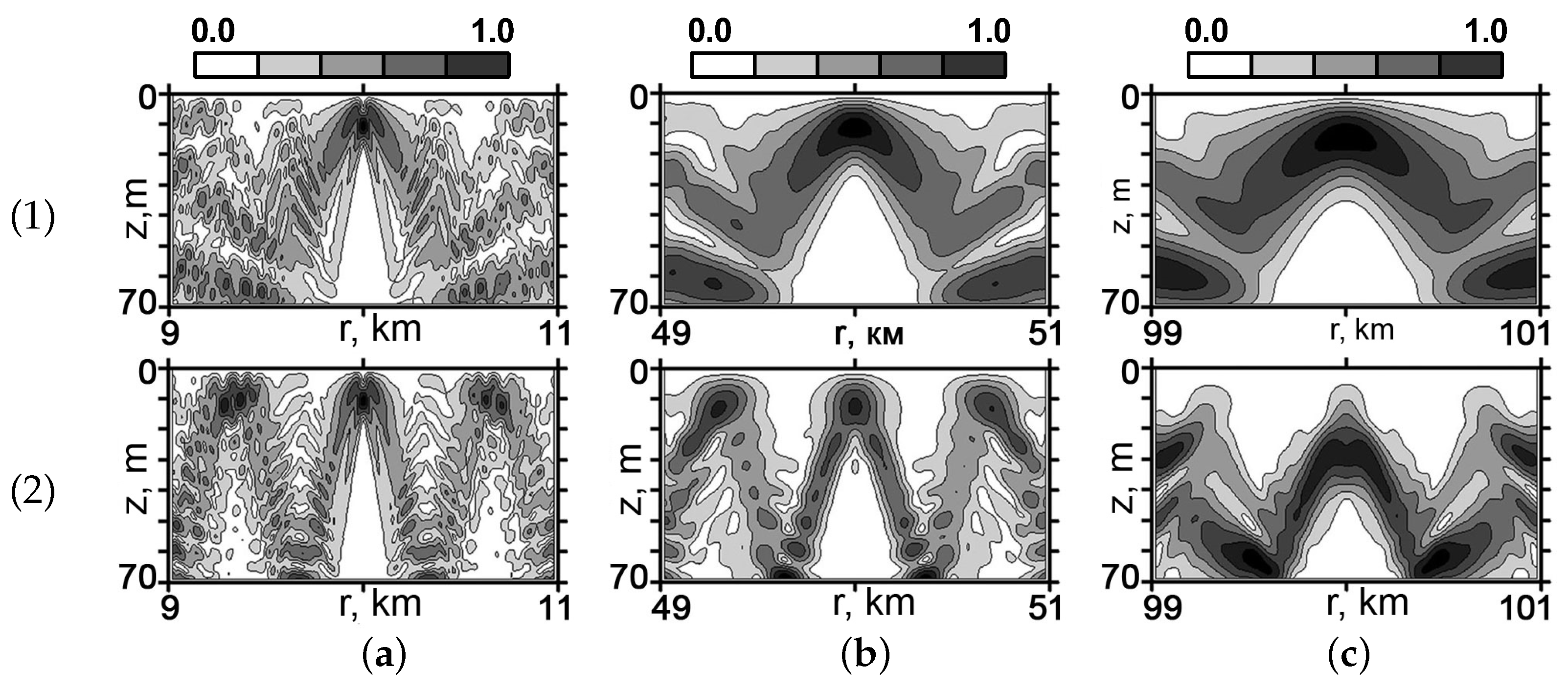
Let us consider the following reference points: $Q_{ij}(r_i,z_j)$, where $r_1=10$ km, $r_2=50$ km, $r_3=100$ km, $z_1=10$ m, $z_2=35$ m, and $z_3=60$ m. The results of the numerical modeling for the reference points $Q_{ij}$ are shown in Figure 4, Figure 5, Figure 6, Figure 7 and Figure 8. Figure 4 and Figure 5 show the brightness patterns of the normalized sound field $\left|\mathsf{\Psi }\right(r,z\left)\right|$ in the vicinity of the localization point $Q_{i_1}(r_i,z_1=10$ m) for the WW and SW at different distances ($r_1=10$ km, $r_2=50$ km, $r_3=100$ km) from the RTA. Figure 4 corresponds to $f_1=150$ Hz and Figure 5 to $f_2=300$ Hz.

As can be seen from Figure 4 and Figure 5, as the distance from the localization point of the field $Q(r_0,z_0)$ increases, the longitudinal and transverse dimensions of the focal spot increase. For example, for the SW at a distance of $r_1=10$ km at a frequency of $f_1=150$ Hz, the dimensions of the focal spot are $\mathsf{\Delta }z=7.7$ m and $\mathsf{\Delta }r=80$ m. For a frequency of $f_2=300$ Hz: $\mathsf{\Delta }z=3.9$ m and $\mathsf{\Delta }r=30$ m. For a distance of $r_3=100$ km and a frequency of $f_1=150$ Hz, the dimensions of the focal spot are $\mathsf{\Delta }z=16.4$ m and $\mathsf{\Delta }r=224$ m. For a frequency of $f_2=300$ Hz: $\mathsf{\Delta }z=9.6$ m and $\mathsf{\Delta }r=126$ m.

A similar behavior of the focal spot parameters was also observed for the WW. This effect is explained by the manifestation of bottom absorption, by which, with increasing distance, the fraction of modes with high numbers, responsible for the small-scale structure of the field, decreases. As a result, the spatial distribution of the field in the localization region becomes smoother with increasing distance. This, in turn, leads to a decrease in the contrast of the focal spot, i.e., a decrease in the focus factor. For an SW at a distance of $r_1=10$ km at a frequency of $f_1=150$ Hz, $g=5.11$, and at a frequency of $f_2=300$ Hz, $g=8.73$. At a distance of $r_3=100$ km at a frequency of $f_1=150$ Hz, $g=2.47$, and at a frequency of $f_2=300$ Hz, $g=4.14$.

Figure 6 shows the dependence of the focusing factor $g\left(r\right)$ (a) and the horizontal size $\mathsf{\Delta }r\left(r\right)$ of the focal spot (b) on the distance to the localization point. The results are related to the SW. Note that such a characteristic decrease of the focusing factor and an increase of the transverse dimension $\mathsf{\Delta }r\left(r\right)$ is practically independent of the depth of the focusing point and the channel stratification.

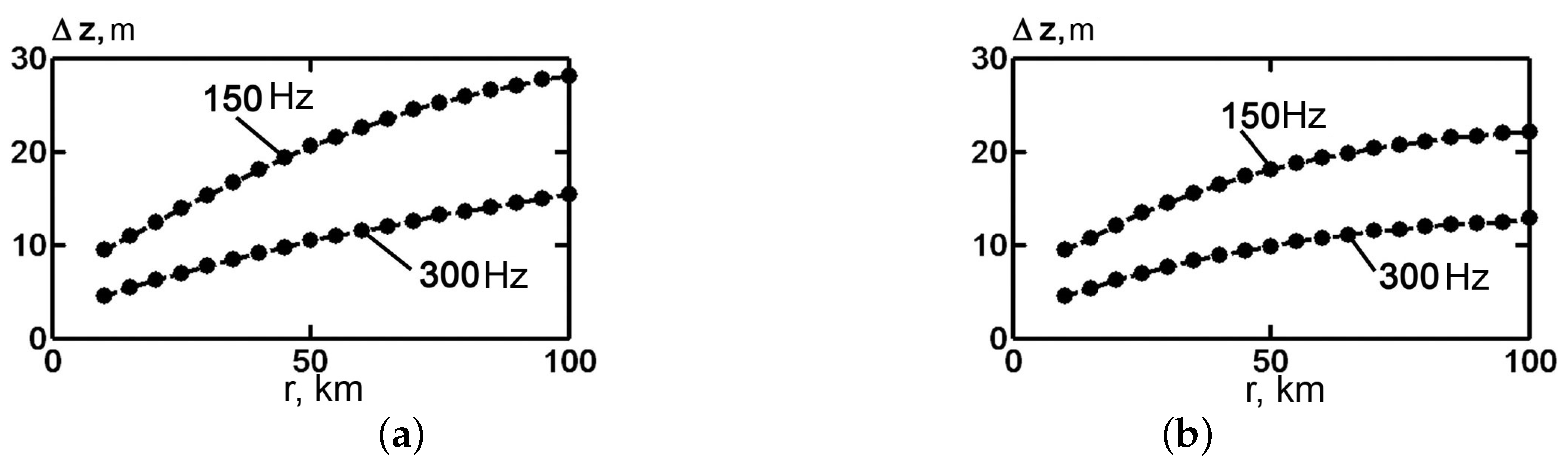
Figure 7 shows the dependence of the longitudinal size $\mathsf{\Delta }z\left(r\right)$ of the focal spot on the distance to the localization point. Figure 7a corresponds to the WW and Figure 7b to the SW. As can be seen, faster growth is observed in the WW than in the SW. This is explained by the less uniform depth distribution of the modes in the waveguide with summer stratification.

In a shallow water waveguide, with the increase of the geometrical dimensions of the focal spot $\mathsf{\Delta }r$, $\mathsf{\Delta }z$ and with the decrease of the focusing factor g, another effect was observed. It consists of the displacement of the focal spot from the position of the localization point in depth. To illustrate this effect, Figure 8 shows the dependence $\delta z\left(r\right)$ on the absolute value of the difference between $z_0$ (the depth of RP Q) and $z_0^{\prime }$ (the depth of the interference maximum closest to Q). As can be seen, the focal spot is most displaced from the RP position near the free surface of the sound channel at frequencies of $f_1=150$ Hz and $f_2=300$ Hz: $Q_{01}(r_0,z_0=10$ m).

Moreover, in the sound channel with summer stratification, this effect is the most pronounced. At a distance of 100 km for a frequency of $f_1=150$ Hz, the shift of the focal spot from $Q(r_0,z_0=10$ m) in the SW is $\mathsf{\Delta }z=27$ m. This is approximately twice as much as compared to the WW, in which $\mathsf{\Delta }z=14$ m. At the same time, at a high frequency $f_2=300$ Hz, the displacement does not exceed two meters in the WW for all considered depths. This situation persists over the entire distance range considered, from 10 km to 100 km. A similar situation was also observed in the SW for localization points below the thermocline, but for $Q(r_0,z_0=10$ m), it increases abruptly to the value of $\mathsf{\Delta }z=17$ m at a distance of 100 km. Such behavior is explained by the manifestation of bottom absorption, by which, with increasing distance, the fraction of high modes decreases. As is known, the high modes form the focal spot near the surface in the SW.

3. Interferogram and Hologram of the Sound Field in the Focusing Point

The intensity of a field of frequency $\omega$ at a horizontal distance r from the source can be represented as the sum of propagating interacting modes:

$$I(r,\omega )=p(r,\omega )p^{*}(r,\omega ),$$

(14)

where

$$p(r,\omega )=\sum _n{C}_n\left(r\right),exp\left[\mathrm{i}{\int }_0^r{q}_n(\omega ,r^{\prime })d{r}^{\prime }\right].$$

Here, $C_n$ is the mode amplitude and $q_n$ is the horizontal wavenumber of the $n-th$ mode. The value $\beta$ determined by the slope angle of the interference lines ${\vartheta }_0$ near the point (${\omega }_0,r_0$) in the range–frequency coordinates has the following form [18]:

$$\beta =\frac{\mathsf{\Delta }\omega /{\omega }_0}{\mathsf{\Delta }r/r_0}=(r_0/{\omega }_0)\mathrm{tg}{\vartheta }_0=-\frac{r_0}{{\omega }_0}\frac{\partial I(r_0,{\omega }_0)/\partial r}{\partial I(r_0,{\omega }_0)/\partial \omega }.$$

(15)

Here, $\mathsf{\Delta }\omega =\omega -{\omega }_0$ and $\mathsf{\Delta }r=r-r_0$ are the frequency and distance increments corresponding to the shift of the considered field extremum on the distance–frequency plane. The value $\beta$ is called the waveguide interference invariant (II) of the sound field.

3.1. Differential Approach

Most work examining various aspects of $\beta$ uses the definition of $\beta$ in terms of a differential approach. As is well known, the conditions of sound propagation in the ocean [18,19] are such that a local interference structure that is resistant to changes in propagation conditions is effectively formed by a small number of constructively interfering modes of the same type. Assuming that the amplitude of the modes is a slower function of their arguments than the phase, one can obtain an expression for the magnitude [18,19]:

$${\beta }_0={\beta }_m\left({\omega }_0\right)=-{\left[\frac{c_{gm}\left({\omega }_0\right)}{c_{pm}\left({\omega }_0\right)}\right]}^2\frac{d{c}_{pm}\left({\omega }_0\right)}{d{c}_{gm}\left({\omega }_0\right)},$$

(16)

where $c_{pm}=\omega /q_m$ and $c_{gm}=d\omega /d{q}_m$ are the phase and group velocities of the reference m-th mode, in the vicinity of which the modes are in phase. As follows from Equation (16), the value thus-determined depends on the number of reference modes m. It should be noted that Equation (16) makes it possible, knowing II, to determine the number of m-th mode, which plays a crucial role in the formation of II.

As an example, consider a typical water layer stratification observed in the shelf region of the ocean—WW and SW (see Figure 3). Figure 9 shows the II value dependencies (${\beta }_m$) on frequency f calculated using Equation (16) for the stratifications shown in Figure 3. From Figure 9, it can be seen that for the WW and SW, the II value ${\beta }_m$ of the first mode is negative and approximately equal, ${\beta }_1\approx -1$. For the WW, all modes ($m=3-12$) have almost the same value, ${\beta }_m\approx 1$. The value ${\beta }_2\approx 0.7$ slightly deviates from this value of 1. In the behavior of ${\beta }_m$ for the SW (Figure 9(1)), there is a clear dependence on the number m. For the group of bottom surface modes (6–12), the behavior of ${\beta }_m$ is similar to the behavior in the WW (${\beta }_m\approx 1$). These bottom surface modes are not very sensitive to the expression of the type of sound speed profile. There is a significant increase in the value of ${\beta }_m$ for the bottom modes in the SW compared to the corresponding modes in the WW (${\beta }_2\approx 1.75$, ${\beta }_3\approx 2.5$, ${\beta }_4\approx 3.0$). As the frequency increases, the mode number $m=5$, which lies at the boundary between the bottom and bottom surface modes, begins to change from one group of modes to another. At the same time, the value ${\beta }_m$ starts to increase. At a certain frequency, it assumes a maximum value and then falls. This behavior of the II modal value ${\beta }_m$ is related to the transformation of the mode in the SW with increasing frequency. The difference in the behavior of the II modal values ${\beta }_m$ should also manifest itself in the different slope of the fringes of the interference structure in the WW and SW. We analyzed this difference in the framework of the integral (spectral) approach [24,25,26,27,28].

3.2. Integral Approach

We considered the sound field intensity distribution $u(r,f)$ (interferogram) Equation (14) in the range–frequency domain $(r,f)$ in the window $r_0-\mathsf{\Delta }r\le r\le r_0+\mathsf{\Delta }r$, $f_0-\mathsf{\Delta }f\le f\le f_0+\mathsf{\Delta }f$:

$$u(r,f)=I(r,f)-\overline{I(r,f)},$$

(17)

where $I(r,f)$—sound field intensity Equation (14). Here, $\overline{I(r,f)}$ denotes the smoothing over the range–frequency window $r_0-\mathsf{\Delta }r\le r\le r_0+\mathsf{\Delta }r$, $f_0-\mathsf{\Delta }f\le f\le f_0+\mathsf{\Delta }f$. We supposed that $u(r,f)=0$ outside of this window. Let us consider a hologram of the sound field $\tilde{u}(\kappa ,\tau )$. The hologram is a result of the two-dimensional Fourier transform (2D-FT) to the interferogram $u(r,f)$ (Equation (17)) in the range–frequency domain $(r,f)$. As an example, the interferogram $u(r,f)$ and the hologram $\tilde{u}(\kappa ,\tau )$ for the SWARM (1995) winter and summer waveguides are presented in Figure 10. Within the framework of the integral approach, the angular distribution $\mathsf{\Phi }\left(\beta \right)$ of the hologram $\tilde{u}(\kappa ,\tau )$ is analyzed.

$$\mathsf{\Phi }\left(\beta \right)={\int }_0^{\infty }{\left|\tilde{u}(\rho cos\vartheta ,\rho sin\vartheta )\right|}^2\rho d\rho ,$$

(18)

where $\kappa =\rho sin\vartheta$; $\tau =\rho cos\vartheta$, $(\rho ,\vartheta )$—polar coordinates in the $(\kappa ,\tau )$ domain; $\beta =(r_0/{\omega }_0)\mathrm{tg}\vartheta$.

The maximum $\mathsf{\Phi }\left(\beta \right)$ falls at the value $\vartheta ={\vartheta }_0$ corresponding to the ${\beta }_0$-II value. The width $\mathsf{\Delta }\beta$ of the function $\mathsf{\Phi }\left(\beta \right)$ (Figure 11) determines the error in specifying the position of the maximum of the function $\mathsf{\Phi }\left(\beta \right)$, i.e., the “blurring” of the direction of observation of the interference fringe. The significance $\mathsf{\Delta }\beta$ increases as the number $\delta l$ of constructively interfering modes decreases. The next width $\mathsf{\Delta }\beta$ was evaluated at the level $0.5\mathsf{\Phi }\left({\beta }_0\right)$.

The width $\mathsf{\Delta }\beta$ in the first approximation is equal to

$$\mathsf{\Delta }\beta =\sqrt{\frac{\mathsf{\Phi }\left(\beta \right)}{d^2\mathsf{\Phi }\left(\beta \right)/d^2\beta }}{|}_{\beta ={\beta }_0}.$$

(19)

The width value $\mathsf{\Delta }\beta$ (Equation (19)) describes the stability of the interference structure of the sound field in the shallow water waveguide. While the width value $\mathsf{\Delta }\beta$ is insignificant, the interference structure of the sound field is stable. While the width value $\mathsf{\Delta }\beta$ becomes more significant, the interference structure of the sound field loses stability. Thus, the value $\mathsf{\Delta }\beta$ can be considered as a measure of the stability of the interference structure of the sound field as a function of distance and frequency variations. The increase in the width value $\mathsf{\Delta }\beta$ is due to two factors. The first is a decrease in the contribution of the high modes (mode attenuation) in the structure of the sound field. The second factor is a decrease in the length of the interference fringes in which the phases of the field modes are preserved.

The results of the analysis of the interference structure in the framework of the integral approach are shown in Figure 12, Figure 13 and Figure 14. These figures show the results of computing the distribution of the normalized dependence $\widehat{\mathsf{\Phi }}\left(\beta \right)=\mathsf{\Phi }\left(\beta \right)/max\left[\mathsf{\Phi }\left(\beta \right)\right]$. Figure 12 corresponds to the WW. Figure 13 corresponds to the SW. Numerical estimates of the values ${\beta }_{0j}$ and $\mathsf{\Delta }{\beta }_j$ corresponding to the dependencies $\mathsf{\Phi }\left(\beta \right)$ in Figure 12 and Figure 13 are given in

Table 1. Values ${\beta }_{0j}$ and $\mathsf{\Delta }{\beta }_j$ corresponding to the dependencies $\mathsf{\Phi }\left(\beta \right)$ in Figure 12.

	(a)	(b)	(c)
(1)	${\beta }_{01}\approx 0.97$, $\mathsf{\Delta }{\beta }_{01}\approx 0.15$	${\beta }_{01}\approx 1.03$, $\mathsf{\Delta }{\beta }_{01}\approx 0.73$	${\beta }_{01}\approx 1.01$, $\mathsf{\Delta }{\beta }_{01}\approx 0.91$
(2)	${\beta }_{02}\approx 0.99$, $\mathsf{\Delta }{\beta }_{02}\approx 0.25$	${\beta }_{02}\approx 0.98$, $\mathsf{\Delta }{\beta }_{02}\approx 0.3$	${\beta }_{02}\approx 1.04$, $\mathsf{\Delta }{\beta }_{02}\approx 0.84$
(3)	${\beta }_{03}\approx 0.97$, $\mathsf{\Delta }{\beta }_{03}\approx 0.23$	${\beta }_{03}\approx 1.01$, $\mathsf{\Delta }{\beta }_{03}\approx 0.24$	${\beta }_{03}\approx 1.03$, $\mathsf{\Delta }{\beta }_{03}\approx 0.52$

and

Table 2. Values ${\beta }_{0j}$ and $\mathsf{\Delta }{\beta }_j$ corresponding to the dependencies $\mathsf{\Phi }\left(\beta \right)$ in Figure 13.

	(a)	(b)	(c)
(1)	${\beta }_{01}\approx 0.98,$ $\mathsf{\Delta }{\beta }_{01}\approx 0.25$	${\beta }_{01}\approx 2.03,$ $\mathsf{\Delta }{\beta }_{01}\approx 1.97$	${\beta }_{01}\approx 2.50,$ $\mathsf{\Delta }{\beta }_{01}\approx 2.02$
(2)	${\beta }_{02}\approx 1.18,$ $\mathsf{\Delta }{\beta }_{02}\approx 0.4$	${\beta }_{02}\approx 1.85,$ $\mathsf{\Delta }{\beta }_{02}\approx 1.73$	${\beta }_{02}\approx 2.47,$ $\mathsf{\Delta }{\beta }_{02}\approx 1.88$
(3)	${\beta }_{03}\approx 0.92,$ $\mathsf{\Delta }{\beta }_{03}\approx 0.4$	${\beta }_{03}\approx 2.15,$ $\mathsf{\Delta }{\beta }_{03}\approx 2.43$	${\beta }_{03}\approx 2.36,$ $\mathsf{\Delta }{\beta }_{03}\approx 2.07$

, respectively. The dependencies of the quantities ${\beta }_{0j}\left(r\right)$ and $\mathsf{\Delta }{\beta }_j\left(r\right)$ on the distance are shown in Figure 14.

Let us consider the results for the WW. The value ${\beta }_0$ for the WW is practically independent of the frequency range and distance. It remains close to ${\beta }_{0j}\approx 1$ throughout the considered range. The value $\mathsf{\Delta }{\beta }_j$ increases with increasing distance. This effect is explained by the “extinction” of modes with high numbers responsible for the small-scale structure of the distribution $u(r,f)$. This leads to an increase in the contribution of modes with low numbers to the field structure responsible for the large-scale structure of the distribution $u(r,f)$. At short distances (∼10 km), the magnitude $\mathsf{\Delta }{\beta }_j$ increases slightly with increasing frequency (see Figure 10(2) and Table 1). Already at a distance (∼50 km), the frequency dependence changes. This is due to the fact that the mode structure shows a faster “depletion” at 100 Hz than at 300 Hz. As a result, at a distance ≥50 km, the width $\mathsf{\Delta }{\beta }_j$ decreases with increasing frequency.

The results corresponding to the SW (Figure 13) demonstrate the complexity of the interference structure of the sound field compared to the WW. In the addition $\mathsf{\Phi }\left(\beta \right)$, several maxima are observed, resulting from the superposition of interference fringes with different tilt angles. These fringes correspond to different groups of modes.

At short distances from the source (∼10 km), the bottom surface modes play a crucial role in the formation of the mode structure of the sound field. As a consequence, at short distances, the quantity ${\beta }_{0j}\approx 1$ over the entire frequency range. As the distance from the source increases, the contribution of the bottom surface modes decreases significantly and the contribution of the bottom modes increases. As a result, at a distance (∼50 km), the II value ${\beta }_{0j}\approx 2$ increases. At such distances, the function $\mathsf{\Phi }\left(\beta \right)$ exhibits, in addition to the main maximum, secondary maxima corresponding to different groups of modes. This is particularly pronounced at higher frequencies (Figure 13(3b)). Over long distances (∼100 km), the sound field is formed only by bottom modes. This leads to an even stronger increase in the magnitude of II: ${\beta }_{0j}\approx 2.5$. In this case, the side maxima of the dependencies $\mathsf{\Phi }\left(\beta \right)$ corresponding to the extinct mode groups disappear. After the distribution $u(r,f)$, they acquire a spotted structure. In this case, the tilt angle of the interference fringes ${\vartheta }_0$ is larger in the SW than in the WW. The value $\mathsf{\Delta }{\beta }_j$ increases with increasing distance. As in the WW, this is due to the “extinction” of modes with high numbers. In the SW, a certain range of distances is observed where $\mathsf{\Delta }{\beta }_j$ increases sharply. For example, for the frequency range $\mathsf{\Delta }{f}_3$ = (350–370) Hz, at a distance ∼50 km, the width reaches $\mathsf{\Delta }{\beta }_3\approx 2.4$. This is due to the fact that, at such distances, the bottom modes and the bottom surface modes make approximately the same contribution to the formation of the sound field. As the distance is further increased, the contribution of the bottom modes becomes dominant. As a result, the width of the function $\mathsf{\Phi }\left(\beta \right)$ decreases to the value $\mathsf{\Delta }{\beta }_j\approx 2$. At short distances (∼10 km), the magnitude $\mathsf{\Delta }{\beta }_j$ increases more with increasing frequency than in the WW. At longer distances (≥50 km), the width $\mathsf{\Delta }{\beta }_j$ decreases with increasing frequency.

The above conclusions were confirmed by the dependence graphs ${\beta }_{0j}$ and $\mathsf{\Delta }{\beta }_j$ from the distance shown in Figure 14 for different frequency ranges.

4. Sound Field Focusing Control by Frequency Tuning

In this section, the results of the work [14] are further developed and the efficiency of controlling the field focusing by frequency tuning in a regular waveguide with different types of water layer stratification (WW and SW) is investigated.

The sound field is localized by the RTA field at frequency $f_0$ at RP $Q_0(r_0,z_0)$. When moving to the point $Q(r,z)$ with frequency $f_0$, the focal spot is destroyed due to the mode dephasing caused by the distance and depth values. The alignment of the mode phases, i.e., the restoration of the sound field focal point, is performed by frequency tuning f ($\delta f=f-f_0$—frequency shift). The frequency tuning allows shifting the undestroyed focal spot to the point $Q(r,z)$ without changing the original distribution of the sound field on the RTA. At the point $Q(r,z)$, the maximum of the sound field $\left|\mathsf{\Psi }\right(Q\left)\right|$ is reached at frequency f. At frequencies deviating from the value f, the sound field value $\left|\mathsf{\Psi }\right(Q\left)\right|$ assumes a lower value.

As an example, we considered a shallow water waveguide (WW and SW) with parameters corresponding to the experiments of JUSREX (1992) [22] and SWARM (1995) [23]. Localization points $Q_{ij}$ ($r_i,z_j$) were placed $r_1=10$ km, $r_2=50$ km, $r_3=100$ km, $z_1=10$ m, $z_2=35$ m, and $z_3=60$ m. The frequency band is $f-\delta f\le f+\delta f$, where $\delta f=10$ Hz. The range domain is $r-\delta r\le r+\delta r$, where $\delta r=2$ km.

The results of modeling the sound field focusing control by frequency tuning are shown in Figure 15, Figure 16, Figure 17, Figure 18, Figure 19, Figure 20 and Figure 21. Figure 15 and Figure 16 show the value distribution of the sound field focused on RP $Q_0(r_0,z_0)$ at reference frequency $f_0$. Figure 15 corresponds to the reference frequency $f_1=150$ Hz and Figure 16 to the reference frequency $f_2=300$ Hz.

It can be seen that the frequency band $\mathsf{\Delta }f$ of the focal spot does not behave monotonically with increasing distance r. First, $\mathsf{\Delta }f$ increases and then decreases. This can be observed especially in the range of higher frequencies. $f_2=300$ Hz. For the WW: $\mathsf{\Delta }{f}_1=1$ Hz, $\mathsf{\Delta }{f}_2=2$ Hz, and $\mathsf{\Delta }{f}_3=1.5$ Hz. For the SW: $\mathsf{\Delta }{f}_1=1.37$ Hz, $\mathsf{\Delta }{f}_2=5.2$ Hz, and $\mathsf{\Delta }{f}_3=3.8$ Hz.

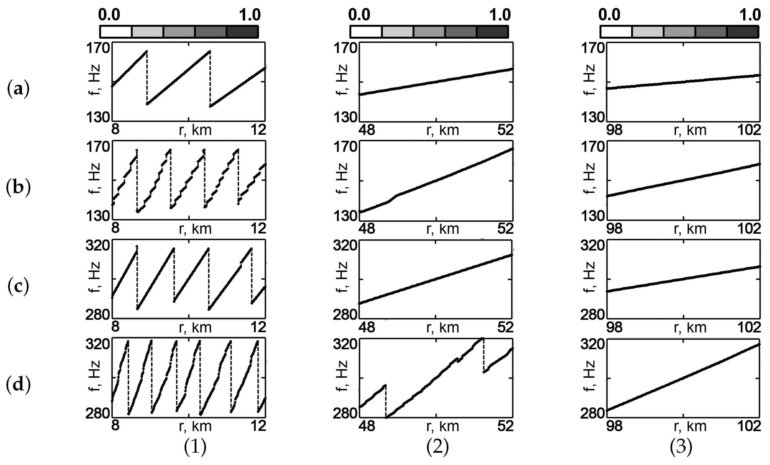
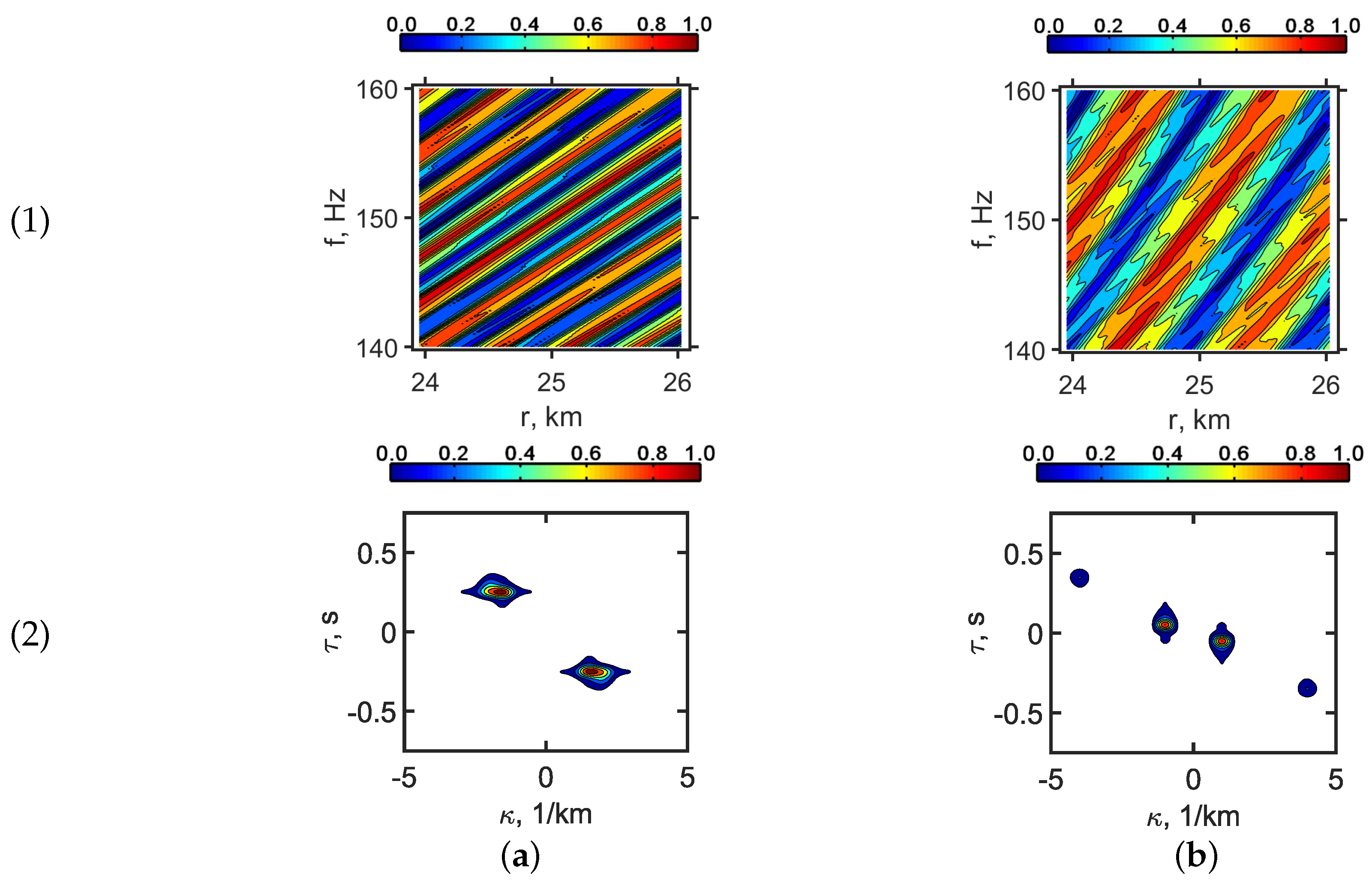
Another feature can be seen in the distributions in Figure 15 and Figure 16. At constant depth, there is a spatial periodicity of the focal points that is most evident in the distributions for distances $r_2=50$ km and $r_3=100$ km. This effect is a consequence of the property of multimode waveguides providing spatially periodic (though somewhat poorer) images [29]. Naturally, the magnitudes of the subsequent focal points gradually become blurred, and the amplitude decreases due to the increasing dephasing of the modes. To illustrate the noticed features of the periodicity of the focal spots, we considered the parameters of the interference structure of the sound field in the coordinates $(r,f)$. The field distributions in the coordinate system $(r,f)$ at the frequency change at depth $z=60$ m are shown in Figure 17. The field localization regions are a sequence of the interference fringes of different slopes due to the periodic repetition of the focal points. The value of II $\beta$ and the space period $D_l$ corresponding to Figure 17 are given in

Table 3. Interference patterns parameters in Figure 17.

	(a)	(b)	(c)
(1)	$\mathrm{tg}\theta \approx 18$ Hz/km, $\beta \approx 1.2$, $D_3\approx 918$ m	$\mathrm{tg}\theta \approx 3$ Hz/km, $\beta \approx 1.0$, $D_3\approx 918$ m	$\mathrm{tg}\theta \approx 1.5$ Hz/km, $\beta \approx 1.0$, $D_3\approx 918$ m
(2)	$\mathrm{tg}\theta \approx 40$ Hz/km, $\beta \approx 2.7$, $D_3\approx 738$ m	$\mathrm{tg}\theta \approx 8$ Hz/km, $\beta \approx 2.7$, $D_3\approx 738$ m	$\mathrm{tg}\theta \approx 4$ Hz/km, $\beta \approx 2.7$, $D_3\approx 738$ m
(3)	$\mathrm{tg}\theta \approx 36$ Hz/km, $\beta \approx 1.2$, $D_3\approx 965$ m,	$\mathrm{tg}\theta \approx 6$ Hz/km, $\beta \approx 1.0$, $D_3\approx 965$ m	$\mathrm{tg}\theta \approx 3$ Hz/km, $\beta \approx 1.0$, $D_3\approx 965$ m
(4)	$\mathrm{tg}\theta \approx 80$ Hz/km, $\beta \approx 2.7$, $D_3\approx 723$ m,	$\mathrm{tg}\theta \approx 16$ Hz/km, $\beta \approx 2.7$, $D_3\approx 723$ m	$\mathrm{tg}\theta \approx 8$ Hz/km, $\beta \approx 2.7$, $D_3\approx 723$ m

.

As can be seen from Figure 17, the angle of the interference fringes $\theta$ decreases with increasing range r. The values $\mathrm{tg}\theta$ for the SW exceed the corresponding values for the WW by more than twice. The same relation was observed for the II value $\beta$ related to the SW and WW.

Figure 18 shows the dependence of the tuning frequency $f\left(r\right)$ on the distance r as the focal spot moves to an arbitrary point $Q(r,z_0)$.

For given dependencies $f\left(r\right)$, radiation frequency tunings are piecewise continuous. The dashed line marks the values of the distance at which the frequency undergoes a jump. The frequency $f\left(r\right)$ was calculated as follows. Along the interference fringe (Figure 17), in the region where the reference point $Q_0(r_0,z_0,f)$ is located, the frequency values f corresponding to the maximum amplitude of the field $\left|\mathsf{\Psi }\right(r,f\left)\right|$ were determined. After passing to the boundaries of the current frequency tuning band f, the transition to the neighboring band was performed with a frequency jump, and along this band, the process of calculating the tuning frequency was repeated, and so on. The $f\left(r\right)$ calculation algorithm was terminated when the limits of the distance change r were reached. Thus, it is possible to control localized fields within a given frequency tuning band by jumping from one band to another. The piecewise continuity of the tuning frequency $f\left(r\right)$ is a consequence of the limited area of the focal spot within which the phase relations are preserved.

At the boundary of the region, the phase undergoes a discontinuity, which causes the frequency jump necessary to compensate for the change in the phases of the modes as they transit to another region of the field focusing. Scanning by focusing occurs on average along straight lines, with slope coefficients $\mathrm{tg}\theta$ decreasing with increasing distance. This property of the evolution of the slope of the straight lines is related to the variance of the II value with respect to the distance and the radiation frequency. This continuous region of focal spots corresponds to a dark band in which the reference point and the reference frequency of the radiation are located in the distributions of Figure 17. There are practically no frequency jumps within this band. The slope coefficients corresponding to these bands are close to the values given above (see Table 3). Thus, scanning with a focal spot in a section of a continuous trajectory is in agreement with the behavior of the II value $\beta$. The frequency of focal spot repetition apparently makes it possible to control localized fields at large distances with a narrow frequency band of the source. The limiting distances are, of course, limited by the width of the interval of constructively interfering modes, which provide an acceptable quality of focusing.

As an example, we show the structure of the field in coordinates $(r,z)$ near the focal spot, shifted by frequency tuning. In Figure 19 is shown the distribution of the sound field for the reference point with coordinates Q(50 km, 60 m). The sound field frequency corresponding to Figure 19 is given in

Table 4. Sound field frequencies corresponding to Figure 19.

	(1)	(2)	(3)
(a)	$f=146$ Hz	$f=150$ Hz	$f=154$ Hz
(b)	$f=142$ Hz	$f=150$ Hz	$f=158$ Hz
(c)	$f=292$ Hz	$f=300$ Hz	$f=308$ Hz
(d)	$f=284$ Hz	$f=300$ Hz	$f=316$ Hz

.

For the value $f_1=150$ Hz, when the focal spot is shifted by a distance of $\pm 1$ km, the frequency must be tuned to $\pm 8$ Hz in the SW and to $\pm 4$ Hz in the WW. For the value $f_2=300$ Hz, the frequency must be tuned to $\pm 16$ Hz in the SW and to $\pm 8$ Hz in the WW. These numerical values of frequency tuning are in good agreement with the parameters of the interference structure of the sound field (Figure 17) in the vicinity of the focal spot. As can be seen from Figure 19, scanning with a focal spot by frequency tuning practically does not change the structure of the sound field in coordinates $(r,z)$ in the vicinity of the focal point.

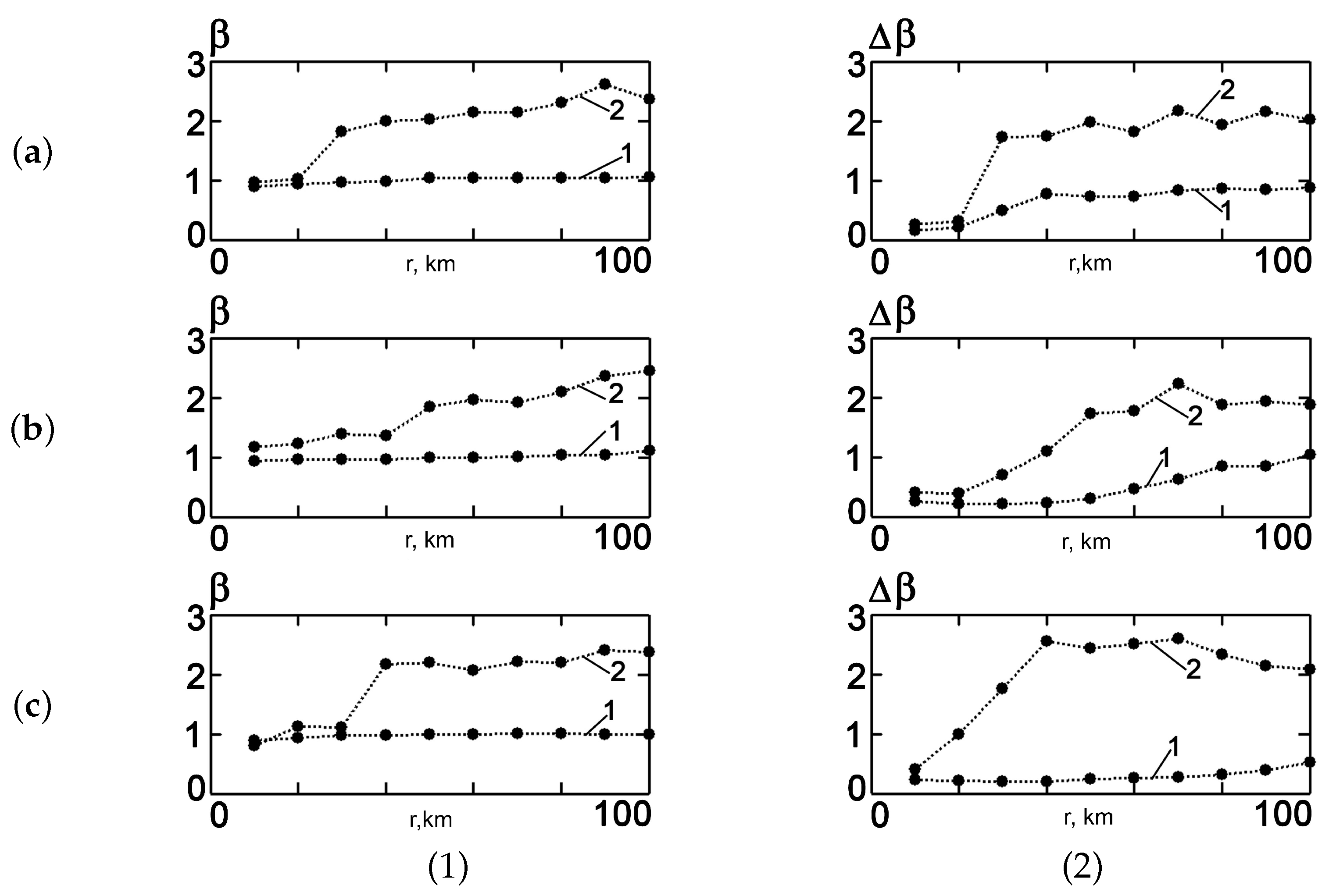
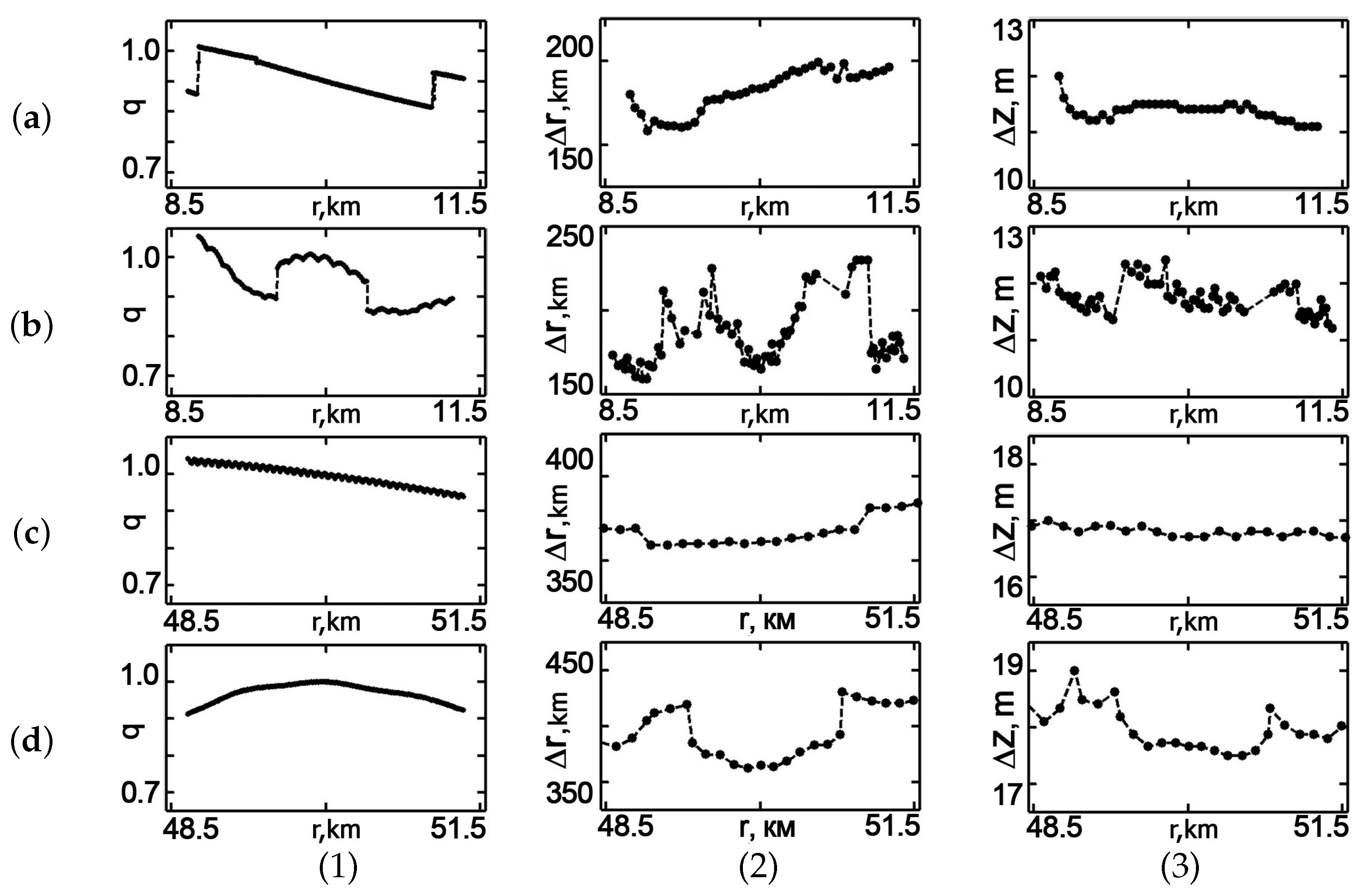
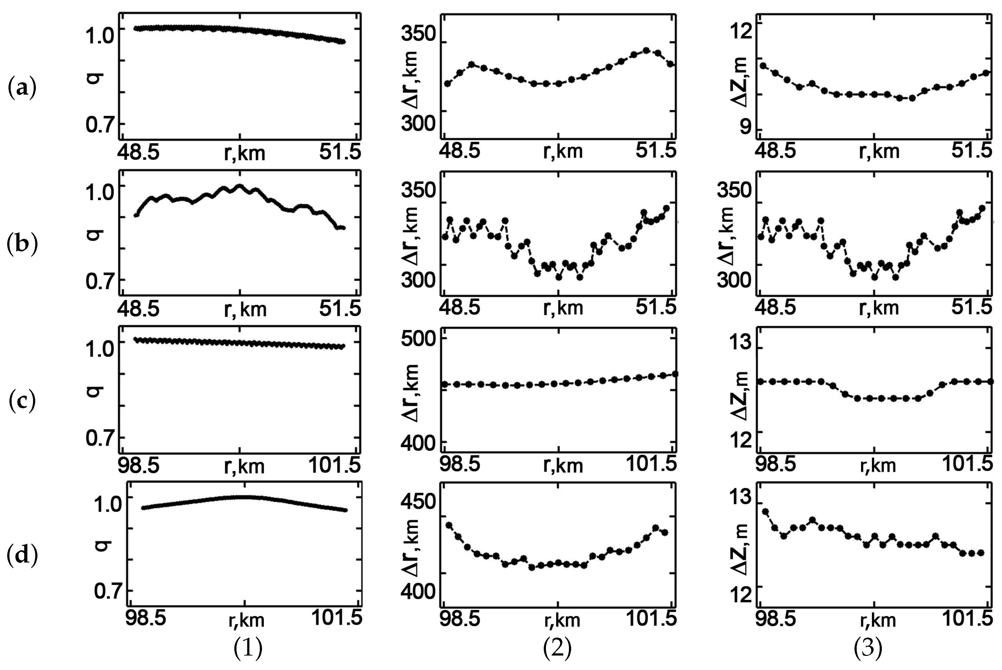
Let us consider the dependence of the focal spot parameters on the scanning distance, taking into account the longitudinal $\mathsf{\Delta }r\left(r\right)$ and transverse $\mathsf{\Delta }z\left(r\right)$ focal spot sizes, as well as the relative focusing factor $q\left(r\right)$. By the relative focusing factor is meant the value:

$$q\left(r\right)=|\mathsf{\Psi }(r,z_0,f\left(r\right))|/|\mathsf{\Psi }(r_0,z_0,f_{1,2})|.$$

(20)

Here, $\left|\mathsf{\Psi }\right(r,z_0,f\left(r\right)\left)\right|$ denotes the field amplitude at a point $Q(r,z_0)$, focused by changing the radiation frequency f; $\left|\mathsf{\Psi }\right(r_0,z_0,f_{1,2}\left)\right|$ is the amplitude of the focused field at the reference point $Q_0$ at the reference frequency $f_{1,2}$. $f_{1,2}$ denotes one of the two cases: $f_1=150$ Hz, $f_2=300$ Hz. The dependence of the focal spot parameters on the distance is shown in Figure 20 and Figure 21. The reference point depth is 60 m.

As can be seen, the parameters of the focal spot are smoother (more stable) during frequency tuning in the WW. This can be explained by the fact that the interference structure in the SW consists of modes with significantly different spatial scales. The focal spot parameters are more stable at low frequencies than at high frequencies. Moreover, the instability of the focal spot parameters decreases with increasing distance from the reference point as the fraction of the bottom surface modes decreases. Regions with strong changes in magnitude q correspond to neighborhoods of tuning frequency jumps f. It should also be noted that the value q increases as the focal spot $Q\ne Q_0$ is shifted forward to the RTA. There are two processes that affect the value of q: the dephasing and the attenuation of the sound modes. The dephasing of the sound modes is due to the shift of the focal spot. The dephasing of the modes leads to a decrease in the focal spot value q for both cases: shift towards the RTA and shift from the RTA. The attenuation of the modes leads to an increase of the focal spot value in the case of a shift towards the RTA and to a decrease of the focal spot value in the case of a shift from the RTA.

The process caused by the modes’ attenuation is stronger than the process caused by the modes’ dephasing for short range ($r=10$ km). As a result, the focal spot shift to the RTA leads an increase of the focal spot value q. In contrast to a short range ($r=10$ km), at a long range ($r=100$ km), the focal spot value $q\left(r\right)$ decreases for both cases: shift forward the RTA and shift from the RTA. This is due to a decrease of the high modes’ contribution (modes’ attenuation) in structure of the sound field with the range increasing.

5. Conclusions

The possibility of controlling localized fields in multimode shallow water waveguides based on the principle of interference invariance was studied. Within the framework of the numerical experiments in a wide frequency range of 100–300 Hz and range intervals of 10–100 km, the possibilities of focusing the sound field by WFR and controlling the focusing of the focal spot by frequency tuning in shallow water waveguides were analyzed. The spatial focusing by WFR consists of recording the sound field from a distant probe source by the RTA, reversing of the recording signals by phase conjugation, and propagating the reversed signal back in a shallow water waveguide. As a result, the sound field is spatially focused at the probe source location. The focal spot scanning was carried out by frequency tuning with a fixed distribution of the sound field at the RTA aperture. A comparative analysis of the features of focusing and focal spot control for summer and winter stratification of the water layer was carried out. It was shown that the focal spot parameters are more stable during frequency tuning in the winter waveguide. It was demonstrated that the sound frequency tuning has a piecewise continuous character and was carried out on a domain of one continuous track and jump passing on another track in accordance with the waveguide interference fringes in the range–frequency domain.

The conclusions presented do not refer to the specific model of this shallow water waveguide. The behavior of the focal spot is qualitatively preserved in different waveguides. The proposed method of controlling the focal spot by frequency tuning is feasible in waveguides that form an interference pattern of the sound field. This means that the criterion for the feasibility of the proposed method is the criterion used for interference invariance [18]. This criterion determines the limits for both the waveguide parameters and the focal spot control range.