

Qualitative Study of the Transport of Microplastics in the Río de la Plata Estuary, Argentina, through Numerical Simulation


Abstract
:1. Introduction
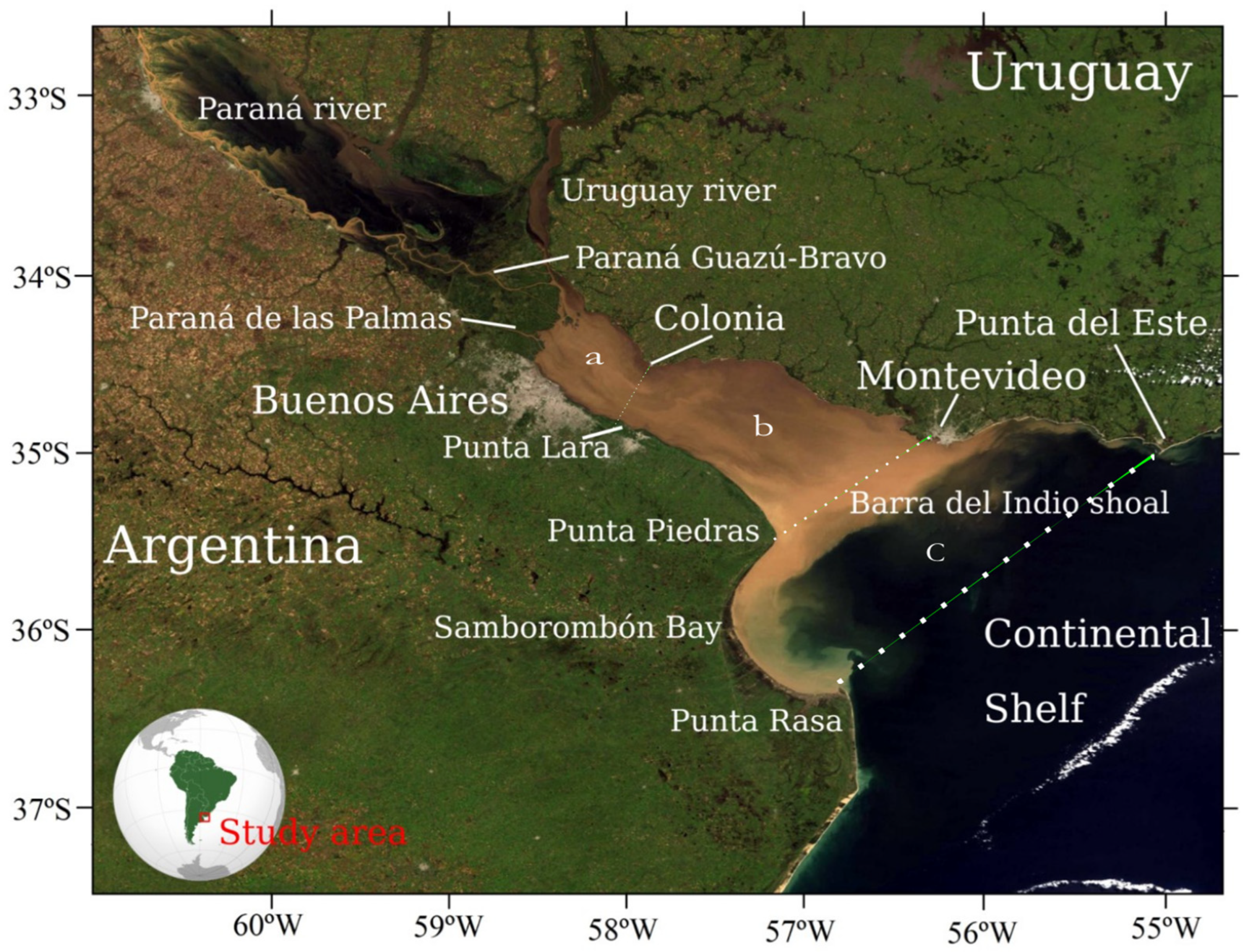
Study Area
2. Methods
2.1. Numerical Model
2.1.1. Hydrodynamic Simulation
2.1.2. Tracking Model
- -
- For sphere
- -
- For cylinders
2.2. Model Configuration
2.2.1. Hydrodynamic Effects
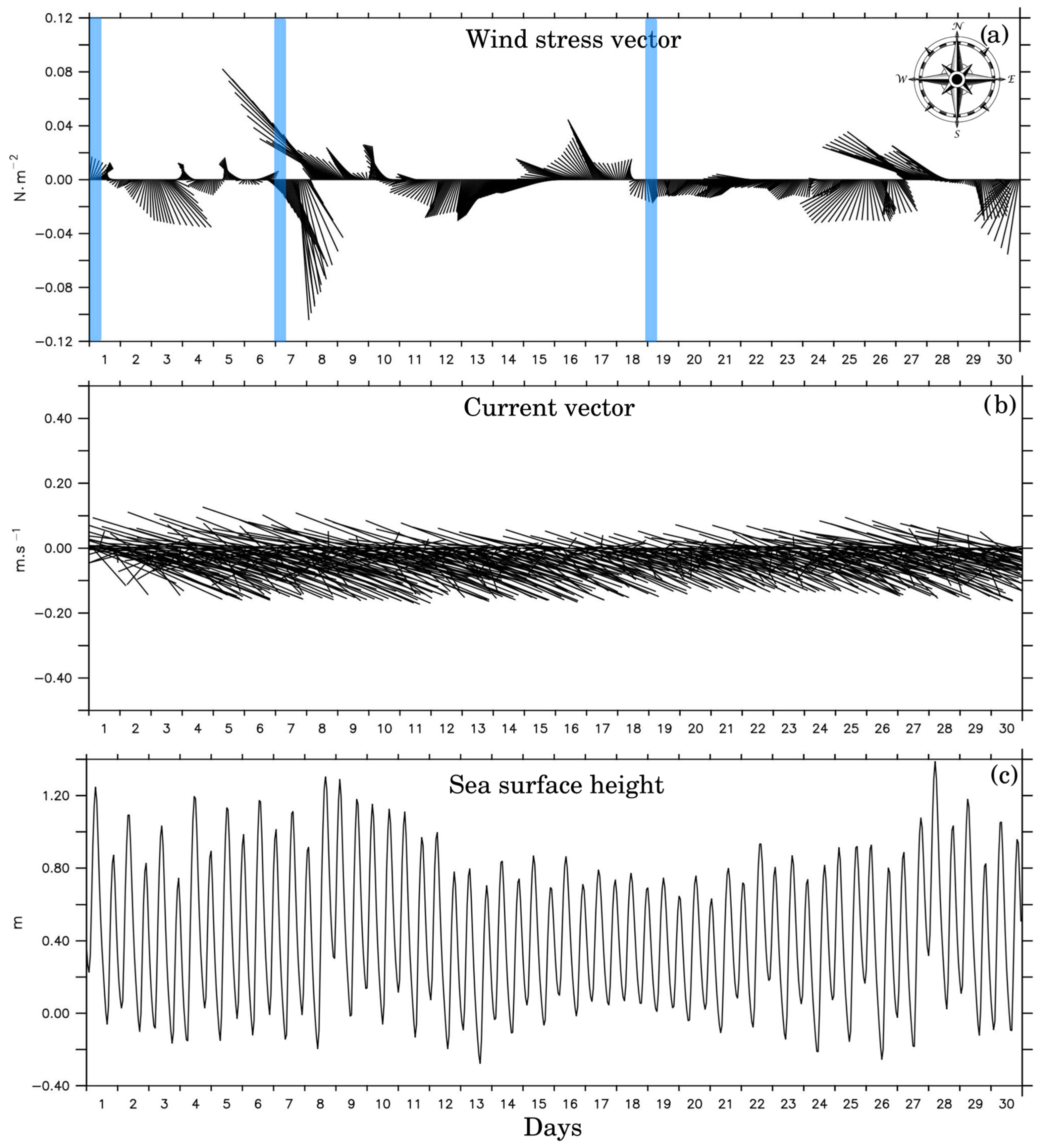
2.2.2. Dependence on Winds
2.2.3. Effect of Morphology
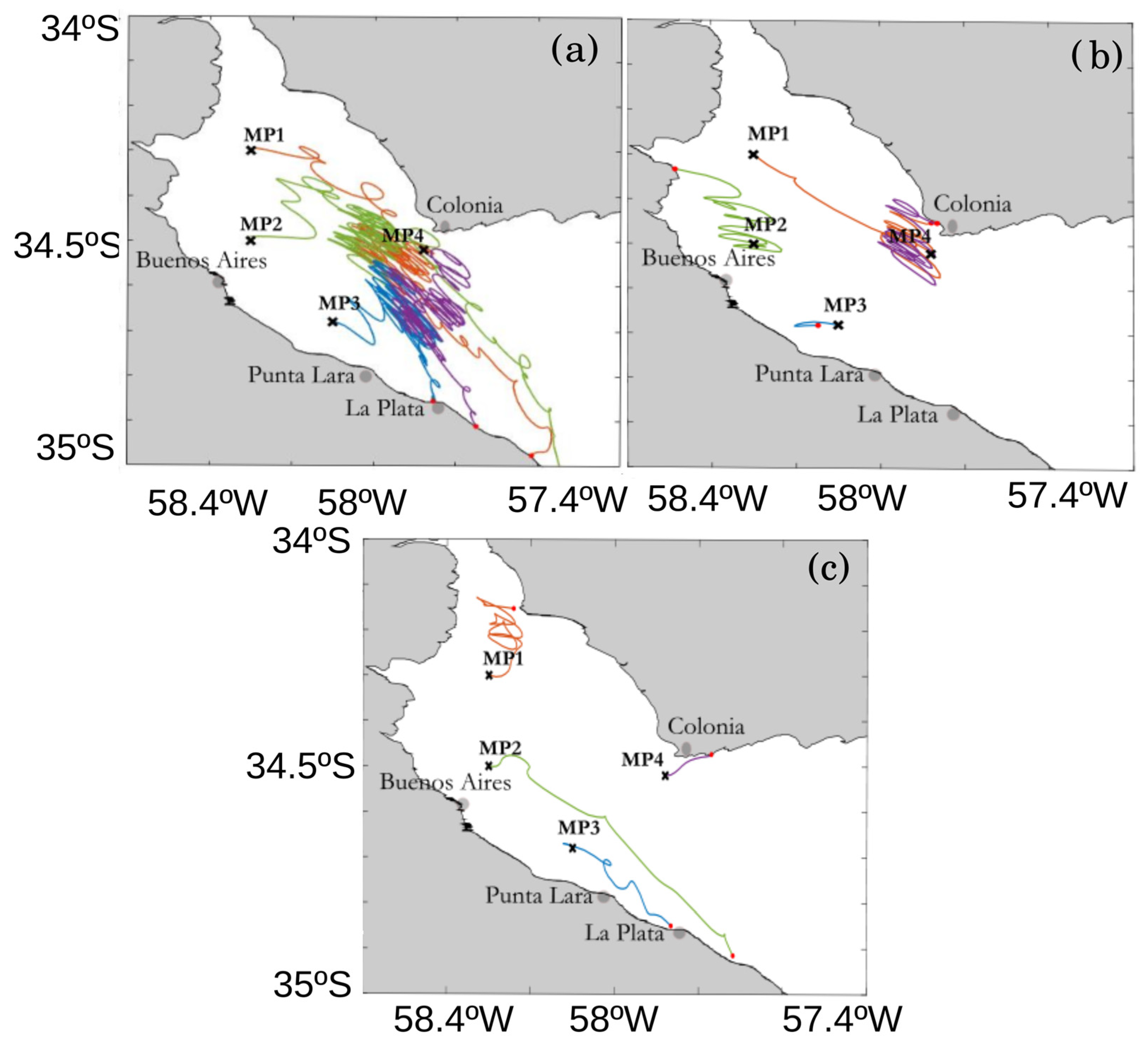
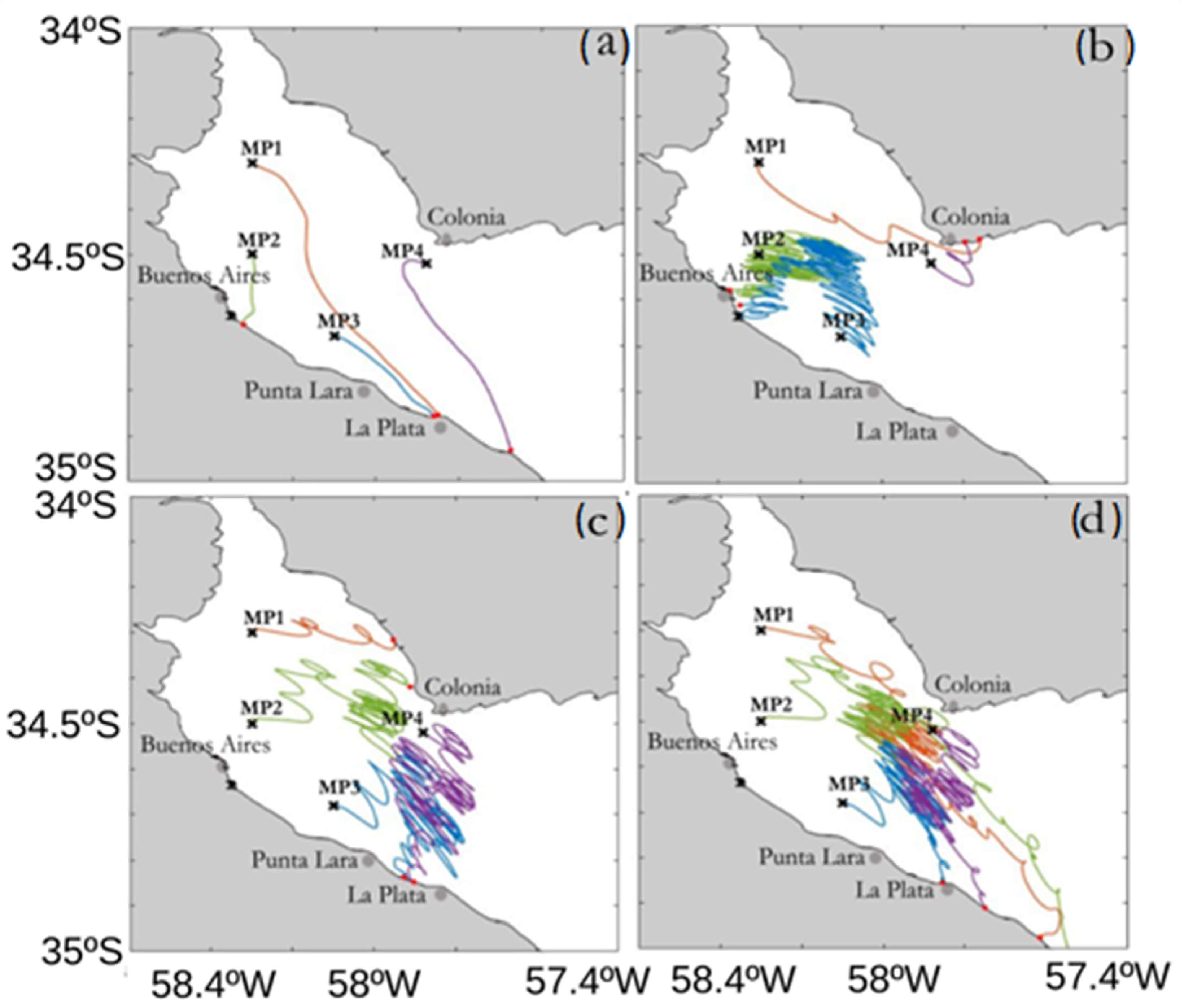
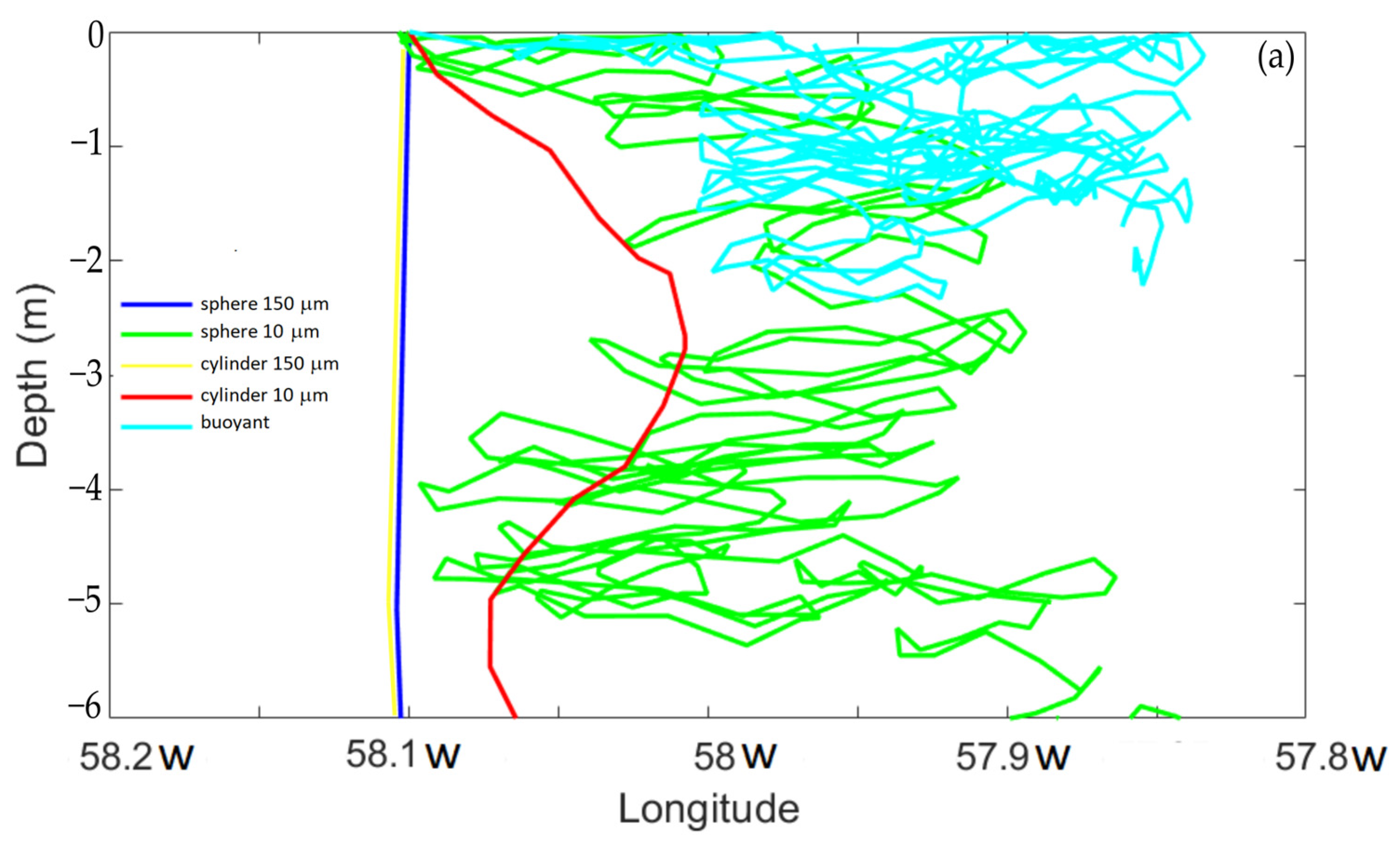
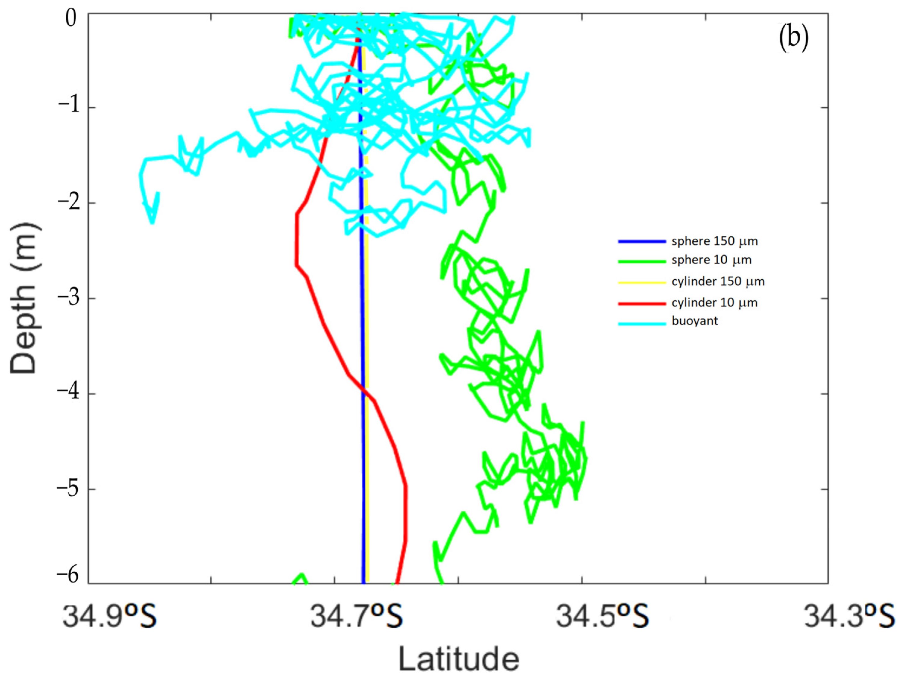
3. Results
3.1. Hydrodynamic Simulation Cases
3.1.1. Hydrodynamic Case I: Effect of the Continental Discharge
3.1.2. Hydrodynamic Case II: Effect of the Continental Discharge Plus Tides
3.1.3. Hydrodynamic Case III: Effect of the Continental Discharge Plus Tides Plus Winds
3.1.4. Hydrodynamic Case IV: Effect of the Continental Discharge Plus Tides Plus Winds Plus Waves
3.1.5. Wind Dependence
3.2. Morphology Effects
4. Discussion
5. Conclusions
Author Contributions
Funding
Institutional Review Board Statement
Informed Consent Statement
Data Availability Statement
Conflicts of Interest
References
- Kane, I.A.; Clare, M.A.; Hodgson, D.M.; Kane, I.A. Dispersion, Accumulation, and the Ultimate Fate of Microplastics in Deep-Marine Environments: A Review and Future Directions. Front. Earth Sci. 2019, 7, 80. [Google Scholar] [CrossRef]
- Petersen, F.; Hubbart, J.A. The Occurrence and Transport of Microplastics: The State of the Science. Sci. Total Environ. 2021, 758, 143936. [Google Scholar] [CrossRef] [PubMed]
- He, J.; Yang, X.; Liu, H. Enhanced Toxicity of Triphenyl Phosphate to Zebrafish in the Presence of Micro- and Nano-Plastics. Sci. Total Environ. 2021, 756, 143986. [Google Scholar] [CrossRef] [PubMed]
- Bermúdez, M.; Vilas, C.; Quintana, R.; Gonzales-Fernandez, D.; Cózar, A.; Diez-Minguito, M. Unravelling Spatio-Temporal Patterns of Suspended Microplastic Concentration in the Natura 2000 Guadalquivir Estuary (SW Spain): Observations and Model Simulations. Mar. Pollut. Bull. 2021, 170, 112622. [Google Scholar] [CrossRef] [PubMed]
- Geyer, R.; Jambeck, J.R.; Law, K.L. Production, Use, and Fate of All Plastics Ever Made. Sci. Adv. 2017, 3, 25–29. [Google Scholar] [CrossRef]
- Luo, W.; Su, L.; Craig, N.J.; Du, F.; Wu, C.; Shi, H.A.C. Comparison of microplastic pollution in different water bodies from urban creeks to coastal waters. Environ. Pollut. 2018, 246, 174–182. [Google Scholar] [CrossRef] [PubMed]
- Chen, X.; Chen, X.; Zhao, Y.; Zhou, H.; Xiong, X.; Wu, C. Effects of Microplastic Biofilms on Nutrient Cycling in Simulated Freshwater Systems. Sci. Total. Environ. 2020, 719, 137276. [Google Scholar] [CrossRef]
- Tursi, A.; Baratta, M.F.; Easton, T.; Chatzisymeon, E.; Chidichimo, F.; De Biase, M.; De Filpo, G. Microplastics in Aquatic Systems, a Comprehensive Review: Origination, Accumulation, Impact, and Removal Technologies. R. Soc. Chem. 2022, 12, 28318–28340. [Google Scholar] [CrossRef]
- Isobe, A.; Uchiyama-Matsumoto, K.; Uchida, K.; Tokai, T. Microplastics in the Southern Ocean. Mar. Pollut. Bull. 2017, 114, 623–626. [Google Scholar] [CrossRef]
- Lu, H.C.; Ziajahromi, S.; Neale, P.A.; Leusch, F.D.L. A Systematic Review of Freshwater Microplastics in Water and Sediments: Recommendations for Harmonisation to Enhance Future Study Comparisons. Sci. Total Environ. 2021, 781, 146693. [Google Scholar] [CrossRef]
- Bom, F.C.; Sá, F. Concentration of Microplastics in Bivalves of the Environment: A Systematic Review. Environ. Monit. Assess. 2021, 193, 1–30. [Google Scholar] [CrossRef] [PubMed]
- Van Sebille, E.; Aliani, S.; Law, K.L.; Maximenko, N.; Alsina, J.M.; Bagaev, A.; Bergmann, M.; Chapron, B.; Chubarenko, I.; Cózar, A.; et al. The Physical Oceanography of the Transport of Floating Marine Debris. Environ. Res. Lett. 2020, 15, 023003. [Google Scholar] [CrossRef]
- Larsen, B.E.; Al-Obaidi, M.A.A.; Guler, H.G.; Carstensen, S.; Goral, K.D.; Christensen, E.D.; Kerpen, N.B.; Schlurmann, T.; Fuhrman, D.R. Experimental Investigation on the Nearshore Transport of Buoyant Microplastic Particles. Mar. Pollut. Bull. 2023, 187, 114610. [Google Scholar] [CrossRef] [PubMed]
- Khatmullina, L.; Chubarenko, I. Transport of Marine Microplastic Particles: Why Is It so Difficult to Predict? Anthr. Coasts 2019, 2, 293–305. [Google Scholar] [CrossRef]
- Hardesty, B.D.; Harari, J.; Isobe, A.; Lebreton, L.; Maximenko, N.; Potemra, J.; Sebille, E.V.; Vethaak, A.D.; Wilcox, C. Using Numerical Model Simulations to Improve the Understanding of Micro-Plastic Distribution and Pathways in the Marine Environment. Front. Mar. Sci. 2017, 4, 1–9. [Google Scholar] [CrossRef]
- Lebreton, L.; Slat, B.; Ferrari, F.; Sainte-Rose, B.; Aitken, J.; Marthouse, R.; Hajbane, S.; Cunsolo, S.; Schwarz, A.; Levivier, A.; et al. Evidence That the Great Pacific Garbage Patch Is Rapidly Accumulating Plastic. Sci. Rep. 2018, 8, 4666. [Google Scholar] [CrossRef]
- Neumann, D.; Callies, U.; Matthies, M. Marine Litter Ensemble Transport Simulations in the Southern North Sea. Mar. Pollut. Bull. 2014, 86, 219–228. [Google Scholar] [CrossRef]
- Critchell, K.; Grech, A.; Schlaefer, J.; Andutta, F.P.; Lambrechts, J.; Wolanski, E.; Hamann, M. Modelling the Fate of Marine Debris along a Complex Shoreline: Lessons from the Great Barrier Reef. Estuar. Coast. Shelf Sci. 2015, 167, 414–426. [Google Scholar] [CrossRef]
- Liubartseva, S.; Coppini, G.; Lecci, R.; Creti, S. Regional Approach to Modeling the Transport of Floating Plastic Debris in the Adriatic Sea. Mar. Pollut. Bull. 2016, 103, 115–127. [Google Scholar] [CrossRef]
- Carlson, D.F.; Suaria, G.; Aliani, S.; Fredj, E.; Fortibuoni, T.; Griffa, A.; Russo, A.; Melli, V. Combining Litter Observations with a Regional Ocean Model to Identify Sources and Sinks of Floating Debris in a Semi-Enclosed Basin: The Adriatic Sea. Front. Mar. Sci. 2017, 4, 78. [Google Scholar] [CrossRef]
- Alsina, J.M.; Jongedijk, C.E.; van Sebille, E. Laboratory Measurements of the Wave-Induced Motion of Plastic Particles: Influence of Wave Period, Plastic Size and Plastic Density. J. Geophys. Res. Oceans 2020, 125, e2020JC016294. [Google Scholar] [CrossRef] [PubMed]
- Guler, H.G.; Larsen, B.E.; Quintana, O.; Goral, K.D.; Carstensen, S.; Christensen, E.D.; Kerpen, N.B.; Schlurmann, T.; Fuhrman, D.R. Experimental Study of Non-Buoyant Microplastic Transport beneath Breaking Irregular Waves on a Live Sediment Bed. Mar. Pollut. Bull. 2022, 181, 113902. [Google Scholar] [CrossRef] [PubMed]
- Passalacqua, G.; Iuppa, C.; Faraci, C. A Simplified Experimental Method to Estimate the Transport of Non-Buoyant Plastic Particles Due to Waves by 2D Image Processing. J. Mar. Sci. Eng. 2023, 11, 1599. [Google Scholar] [CrossRef]
- Jalón-Rojas, I.; Wang, X.H.; Fredj, E. A 3D Numerical Model to Track Marine Plastic Debris (TrackMPD): Sensitivity of Microplastic Trajectories and Fates to Particle Dynamical Properties and Physical Processes. Mar. Pollut. Bull. 2019, 141, 256–272. [Google Scholar] [CrossRef]
- Cheng, M.L.H.; Lippmann, T.C.; Dijkstra, J.A.; Bradt, G.; Cook, S.; Choi, J.; Brown, B.L. A Baseline for Microplastic Particle Occurrence and Distribution in Great Bay Estuary. Mar. Pollut. Bull. 2021, 170, 112653. [Google Scholar] [CrossRef] [PubMed]
- Siegfried, M.; Koelmans, A.A.; Besseling, E.; Kroeze, C. Export of Microplastics from Land to Sea. A Modelling Approach. Water Res. 2017, 127, 249–257. [Google Scholar] [CrossRef]
- Carreto, J.I.; Montoya, N.G.; Akselman, R.; Roja, P.M. Proyecto “Protección Ambiental del Río de la Plata y su Frente Marítimo: Prevención y Control de la Contaminación y Restauración de Hábitats”. RLA 2004, 99, G31. [Google Scholar]
- Simionato, C.G.; Vera, C.S.; Siegismund, F.; Beach, W.P.; Simionato, C.G.; Vera, C.S.; Siegismund, F. Surface Wind Variability on Seasonal and Interannual Scales Over Río de La Plata Area Surface Wind Variability on Seasonal and Interannual Scales Over Rı ´ o de La Plata Area. J. Coast. Res. 2005, 214, 770–783. [Google Scholar] [CrossRef]
- Pazos, R.S.; Amalvy, J.; Pecile, A.; Cochero, J.; Gomez, N. Temporal Patterns in the Abundance, Type and Composition of Microplastics on the Coast of the Río de La Plata Estuary. Mar. Pollut. Bull. 2021, 168, 112382. [Google Scholar] [CrossRef]
- Arias, A.H.; Ronda, A.C.; Oliva, A.L.; Marcovecchio, J.E. Evidence of Microplastic Ingestion by Fish from the Bahía Blanca Estuary in Argentina, South America. Bull. Environ. Contam. Toxicol. 2019, 102, 750–756. [Google Scholar] [CrossRef]
- Balay, M.A. El Río de La Plata Entre La Atmósfera y El Mar. H-621 B. Aires Serv. Hidrogr. Nav. Armada Argent. 1961, 153. [Google Scholar]
- Borús, J.; Giacosa, J. Evaluación de Caudales Diarios Descargados Por Los Grandes Ríos Del Sistema Del Plata al Río de La Plata. In Direccion y Alerta Hidrológico; Instituto Nacional del Agua: Ezeiza, Argentina, 2014. [Google Scholar]
- Borús, J.; Uriburu Quirno, M.; Calvo, D. Evaluación de Caudales Diarios Descargados 470 Por Los Grandes Ríos del Sistema del Plata al Estuario del Río de la Plata, Dirección de Sistemas de Información y Alerta Hidrológico; Instituto Nacional del Agua: Ezeiza, Argentina, 2017. [Google Scholar]
- Simionato, C.G. Estudio de La Dinámica Hidro-Sedimentológica-Del Río de La Plata. Proyecto FREPLATA 2011, 99, G31. [Google Scholar]
- Ottoman, F.; Urien, C.M. Sur Quelques Problemes Sedimentologiques Dans Le Río de La Plata. Rev. Géographie Phys. Géologie Dyn. 1996, 209–224. [Google Scholar]
- Parker, G.; Cavalloto, J.L.; Marcolini, S.; Violante, R. Los Registros Acústicos en la Diferenciación de Sedimentos Subácueos Actuales (Río de La Plata); 1986; pp. 32–44. [Google Scholar]
- Siomionato, C.G.; Meccia, V.L.; Guerrero, R.A.; Dragani, W.C.; Nuñez, M.N. The Río de La Plata Estuary Response to Wind Variability in Synoptic to Intra-Seasonal Scales: II Currents Vertical Structure and Its Implications on the Salt Wedge Structure. J. Geophys. Res. Oceans 2007, 112, C07005. [Google Scholar] [CrossRef]
- Simionato, C.G.; Dragani, W.C.; Nuñez, M.N.; Engel, M. A Set of 3-D Nested Models for Tidal Propagation from the Argentinean Continental Shelf to the Río de La Plata Estuary—Part I M2. J. Coast. Res. 2004, 20, 893–912. [Google Scholar] [CrossRef]
- Guerrero, R.A.; Acha, E.M.; Framiñan, M.B.; Lasta, C. Physical Oceanography of the Río de La Plata Estuary, Argentina. Cont. Shelf Res. 1997, 17, 727–742. [Google Scholar] [CrossRef]
- Meccia, V.L.; Simionato, C.G.; Guerrero, R.A. The Río de la plata estuary response to wind variability in synoptic timescale: Salinity fields and salt wedge structure. J. Coast. Res. 2013, 29, 61–77. [Google Scholar] [CrossRef]
- Simionato, C.; Dragani, W.C.; Meccia, V.L.; Nuñez, M.N. A Numerical Study of the Barotropic Circulation of the Río de La Plata Estuary: Sensitivity to Bathymetry, Earth Rotation and Low Frequency Wind Variability. Estuar. Coast. Shelf Sci. 2004, 61, 261–273. [Google Scholar] [CrossRef]
- Jaime, P.R.; Menéndez, Á.N. Vinculación Entre ElCaudal Del Río Paraná yEl Fenómeno de El Niño. Instituto Nacional del Agua. 2003. Available online: https://repositorio.ina.gob.ar/handle/123456789/462 (accessed on 20 November 2023).
- Jaime, P.R.; Menéndez, Á.N. Modelo Hidrodinámico “Ríode La Plata 2000”. Report LHA-INA 183-01-99, INA. 1999. Available online: https://repositorio.ina.gob.ar/handle/123456789/92 (accessed on 20 November 2023).
- Magni, L.F.; Castro, L.N.; Rendina, A.E. Evaluation of Heavy Metal Contamination Levels in River Sediments and Their Risk to Human Health in Urban Areas: A Case Study in the Matanza-Riachuelo Basin, Agentina. Environ. Res. 2021, 197, 110979. [Google Scholar] [CrossRef]
- O’Farrell, I.; Lombardo, R.; Tezanos, P.; Loez, C. The Assessment of Water Quality in the Lower Luján River (Buenos Aires, Argentina): Phytoplankton and Algal Bioassay. Environ. Pollut. 2002, 20, 207–218. [Google Scholar] [CrossRef]
- Moreira, D.; Simionato, C.G. Modeling the Suspended Sediment Transport in a Very Wide, Shallow, and Microtidal Estuary, the Río de La Plata, Argentina. J. Adv. Model. Earth Syst. 2019, 11, 3284–3304. [Google Scholar] [CrossRef]
- Minetti, J.L.; Vargas, W.M. Comportamiento Del Borde Antiticiclónico Subtropical En Sudamérica. Rev. Geofísica 1990, 177–190. [Google Scholar]
- Simionato, C.; Meccia, V.L.; Dragani, W.C.; Nuñez, M.N. On the Use of the NCEP/NCAR Surface Winds for Modeling Barotropic Circulation in the Río de La Plata Estuary. Estuar. Coast. Shelf Sci. 2006, 70, 195–206. [Google Scholar] [CrossRef]
- Vera, C.S.; Vigliarolo, P.K.; Berbery, E.H. Cold Season Synoptic Scale Waves over Subtropical South America. Mon. Weather Rev. 2002, 130, 684–699. [Google Scholar] [CrossRef]
- Dragani, W.C.; Romero, S.I. Impact of a Possible Local Wind Change on the Wave Climate in the Upper Río de La Plata. Int. J. Climatol. 2004, 24, 1149–1157. [Google Scholar] [CrossRef]
- Lazure, P.; Dumas, F. An External-Internal Mode Coupling for a 3D Hydrodynamical Model for Applications at Regional Scale (MARS). Adv. Water Resour. 2008, 31, 233–250. [Google Scholar] [CrossRef]
- Lazure, P.; Salomon, J.C. Coupled 2-D and 3-D Modelling of Coastal Hydrodynamics. Oceanol. Acta 1991, 14, 173–180. [Google Scholar]
- Andre, G.; Garreau, P.; Garnier, V.; Fraunié, P. Modelled Variability of the Sea Surface Circulation in the North-Western Mediterranean Sea and in the Gulf of Lions. Ocean Dyn. 2005, 55, 294–308. [Google Scholar] [CrossRef]
- Pous, S. Dynamique Océanique Dans Les Golfes Persique et d’Oman, Phdthesis, Université de Bretagne Occidentale. 2005. Available online: https://theses.hal.science/tel-01301686 (accessed on 20 November 2023).
- Fossati, M.; Piedra-Cueva, I. A 3D Hydrodynamic Numerical Model of the Río de La Plata and Montevideo’s Coastal Zone. Appl. Math. Model. 2013, 37, 1310–1332. [Google Scholar] [CrossRef]
- Moreira, D. Estudio de Los Procesos Que Determinan El Transporte de Los Sedimentos Finos y Su Variabilidad En El Río de La Plata En Base a Simulaciones Numéricas y Observaciones Satelitales e in Situ. Phdthesis Universidad de Buenos Aires, Facultad de Ciencias Exactas y Naturales, Buenos Aires, Argentina. 2016. Available online: https://hdl.handle.net/20.500.12110/tesis_n6101_Moreira (accessed on 20 November 2023).
- Simionato, C.; Meccia, V.L.; Dragani, W.C. On the Path of Plumes of the Río de La Plata Estuary Main Tributaries and Their Mixing Scales. GEOACTA 2009, 34, 87–116. [Google Scholar]
- Jaime, P. Analisis Del Regimen Hidrologico de Los Rios Parana y Uruguay. Prot. Ambient. Rio Plata Su Frente Maritimo Prev. Control Contam. Restaur. Habitats 2002, 53, 160. [Google Scholar]
- Enders, K.; Lenz, R.; Stedmon, C.A.; Nielsen, T.G. Abundance, Size and Polymer Composition of Marine Microplastics ≥10 Μm in the Atlantic Ocean and Their Modelled Vertical Distribution. Mar. Pollut. Bull. 2015, 100, 70–81. [Google Scholar] [CrossRef] [PubMed]
- Plastic Europe. Plastics—The Facts 2019. Plastics Europe AISBL. Brussel, Belgium. 2019. Available online: https://plasticseurope.org/wp-content/uploads/2021/10/2019-Plastics-the-facts.pd. (accessed on 20 November 2023).
- Rodrigues, S.M.; Almeida, C.M.R.; Silva, D.; Cunha, J.; Antunes, C.; Freitas, V.; Ramos, S. Science of the Total Environment Microplastic Contamination in an Urban Estuary: Abundance and Distribution of Microplastics and Fi Sh Larvae in the Douro Estuary. Sci. Total Environ. 2019, 659, 1071–1081. [Google Scholar] [CrossRef]
- Moreira, D.; Simionato, C.; Re, M.; Gerbec, M.S.; Cayocca, F.; Fossati, M. Implementación de Un Modelo Numérico Para El Estudio Del Transporte de Sedimentos Finos En El Río de La Plata. In Proceedings of the IFRH 2012-Primer Encuentro de Investigadores en Formación en Recursos Hídricos, Buenos Aires, Argentina, 14–15 June 2012. [Google Scholar]
- Feng, Q.; An, C.; Chen, Z.; Lee, K.; Zheng, W. Identification of the Driving Factors of Microplastic Load and Morphology in Estuaries for Improving Monitoring and Management Strategies: A Global Meta-Analysis. Environ. Pollut. 2023, 333, 122014. [Google Scholar] [CrossRef] [PubMed]
- Lentz, S.; Fewings, M.R. The Wind- and Wave-Driven Inner-Shelf Circulation. Annu. Rev. Mar. Sci. 2012, 4, 317–343. [Google Scholar] [CrossRef] [PubMed]
- Diez-Minguito, M.; Bermúdez, M.; Gago, J.; Carretero, O.; Viña, L. Observations and Idealized Modelling of Microplastic Transport in Estuaries: The Exemplary Case of an Upwelling System (Ría de Vigo, NW Spain). Mar. Chem. 2020, 222, 103780. [Google Scholar] [CrossRef]
- Lawrence, C.; Neff, J. The Contemporary Physical and Chemical Flux of Aeolian Dust: A Synthesis of Direct Measurements of Dust Deposition. Chem. Geol. 2009, 267, 46–63. [Google Scholar] [CrossRef]
- Elagami, H.; Ahmadi, P.; Fleckenstein, J.H.; Frei, S.; Obst, M.; Agarwal, S.; Gilfedder, B.S. Measurement of Microplastic Settling Velocities and Implications for Residence Times in Thermally Stratified Lakes. Limnol. Oceanogr. 2022, 67, 934–945. [Google Scholar] [CrossRef]
- Laursen, S.N.; Fruergaard, M.; Dodhia, M.S.; Posth, N.R.; Rasmussen, M.B.; Larsen, M.N.; Shilla, D.; Shilla, D.; Kilawe, J.J.; Kizenga, H.J.; et al. Settling of Buoyant Microplastic in Estuaries: The Importance of Flocculation. Sci. Total Environ. 2023, 886, 163976. [Google Scholar] [CrossRef]


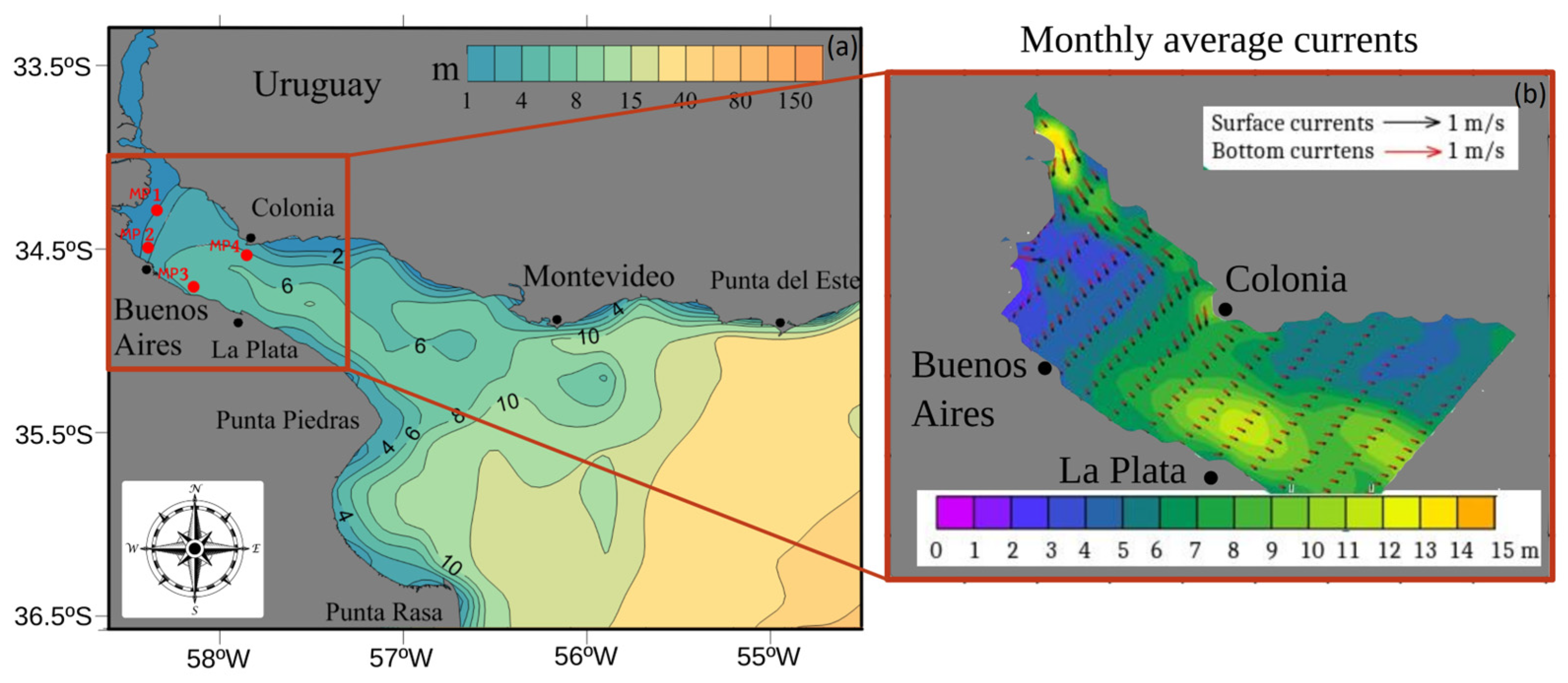
| MPs | Location: Lon, Lat | Reference |
|---|---|---|
| MP1 | 58.3° W, 34.3° S | Playa Honda, influenced by the tributary rivers’ discharge (Uruguay and Paraná Guazú-Bravo). |
| MP2 | 58.3° W, 34.5° S | Playa Honda, influenced by the tributary rivers’ discharge (Uruguay and Paraná Guazú-Bravo). |
| MP3 | 58.1° W, 34.68° S | Berazategui, near the plant of water effluent treatment (AySA). |
| MP4 | 57.88° W, 34.52° S | Near Colonia del Sacramento. |
Disclaimer/Publisher’s Note: The statements, opinions and data contained in all publications are solely those of the individual author(s) and contributor(s) and not of MDPI and/or the editor(s). MDPI and/or the editor(s) disclaim responsibility for any injury to people or property resulting from any ideas, methods, instructions or products referred to in the content. |
© 2023 by the authors. Licensee MDPI, Basel, Switzerland. This article is an open access article distributed under the terms and conditions of the Creative Commons Attribution (CC BY) license (https://creativecommons.org/licenses/by/4.0/).
Share and Cite
Elisei Schicchi, A.; Moreira, D.; Eisenberg, P.; Simionato, C.G. Qualitative Study of the Transport of Microplastics in the Río de la Plata Estuary, Argentina, through Numerical Simulation. J. Mar. Sci. Eng. 2023, 11, 2317. https://doi.org/10.3390/jmse11122317
Elisei Schicchi A, Moreira D, Eisenberg P, Simionato CG. Qualitative Study of the Transport of Microplastics in the Río de la Plata Estuary, Argentina, through Numerical Simulation. Journal of Marine Science and Engineering. 2023; 11(12):2317. https://doi.org/10.3390/jmse11122317
Chicago/Turabian StyleElisei Schicchi, Alejandra, Diego Moreira, Patricia Eisenberg, and Claudia G. Simionato. 2023. "Qualitative Study of the Transport of Microplastics in the Río de la Plata Estuary, Argentina, through Numerical Simulation" Journal of Marine Science and Engineering 11, no. 12: 2317. https://doi.org/10.3390/jmse11122317
APA StyleElisei Schicchi, A., Moreira, D., Eisenberg, P., & Simionato, C. G. (2023). Qualitative Study of the Transport of Microplastics in the Río de la Plata Estuary, Argentina, through Numerical Simulation. Journal of Marine Science and Engineering, 11(12), 2317. https://doi.org/10.3390/jmse11122317