Article

On the Digital Twin of The Ocean Cleanup Systems—Part I: Calibration of the Drag Coefficients of a Netted Screen in OrcaFlex Using CFD and Full-Scale Experiments

by
Martin Alejandro Gonzalez Jimenez
,
Andriarimina Daniel Rakotonirina
*,
Bruno Sainte-Rose
and
David James Cox
The Ocean Cleanup, Coolsingel 6, 3011 AD Rotterdam, The Netherlands
*
Author to whom correspondence should be addressed.
J. Mar. Sci. Eng. 2023, 11(10), 1943; https://doi.org/10.3390/jmse11101943
Submission received: 31 July 2023 / Revised: 18 September 2023 / Accepted: 18 September 2023 / Published: 8 October 2023

Abstract

:
The Ocean Cleanup introduces a Digital Twin (DT) describing the cleanup systems made of netting to extract marine litter from our oceans. It consists of two wings forming a “U-shape” and a retention zone. During operation, the system is towed and drag-driven with a span-to-length ratio of 0.6 S R * 0.8. The twine Reynolds number is R e t * [ 800 : 1600 ] , making it experience various local drag coefficients. The DT was built with OrcaFlex (OF) aiming at: (i) avoiding over- or under-designing the system; (ii) supporting the scale-up of the system; and (iii) estimating the costs and/or the impact of our offshore operations. Therefore, we present an attempt to build an accurate DT using data from the Great Pacific Garbage Patch (GPGP). We developed a three-cycle validation: (i) initial guess applying Naumov’s semi-empirical drag coefficient to define the OF drag coefficients without the influence of the angles of attack θ of the wings; (ii) adjustment of the OF drag coefficients using AquaSim (AS) with its twine-by-twine drag correlation for various θ ; (iii) re-adjustment of the OF drag coefficients from two-dimensional CFD simulations using Direct Numerical Simulation (DNS) for a twine-by-twine establishment of a drag correlation on a 1 m plane net, highlighting the shielding effects for θ < 24 ° . Consequently, an initial underestimation of −3% in the combined towline tension, for a nominal span ( S R * = 0.6 ), was corrected to a slight overestimation of +7% compared to the GPGP data. For a wide span ( S R * = 0.8 ), the deviation remained between +1% and +15% throughout the validation process. For a narrow span ( S R * 0.02), mostly exhibiting low θ , the first cycle showed a +276% deviation, whereas at the end of the third cycle, it showed a +43% deviation.

1. Introduction

In July 2021, a new design of our cleanup system called System 002, also known as “Jenny”, was deployed in the GPGP for a testing campaign. It replaced System 001, which consisted of a 600 m-long passive floating barrier with a 3 m-deep skirt, designed to take advantage of natural oceanic forces, such as currents and winds, to passively capture plastic waste. As opposed to System 001, Jenny was designed to be a 800 m towed (i.e., active propulsion) floating structure composed of a containment boom and a permeable net-like skirt generally inspired by the fishing industry. As a matter of fact, the centuries of existence of fishing and aquaculture have set the ground for the development of most ocean applications involving net-like devices. In essence, the existing knowledge is directly extrapolated onto new technologies along with some additional fine-tuning. In this context, the netting, considered as a basic element of most fishing gears, has been subjected to numerous investigations. Specially, the studies on the hydrodynamic characteristics of the netting highlight the necessity of optimizing them for efficiency purposes.
In the specific case of The Ocean Cleanup, the engineering efficiency and the environmental efficiency are the main drivers of the cleanup project, and they translate into two Key Performance Indicators (KPIs): the costs per kilogram of extracted plastic and the CO 2 emission per kilogram of extracted plastic. Being a Non-profit organization that supports the preservation of marine ecosystems, The Ocean Cleanup is committed to making efficient use of the obtained donations, by setting a cost KPI target that aims to become financially self-sustaining and minimize the environmental impact of its operations, by setting an environmental KPI target that can lead to a net positive environmental impact. Therefore, understanding the hydrodynamic loads acting on its cleanup systems, which impact the fuel consumption of the towing vessels (implicitly their CO 2 emission), becomes imperative. This is especially relevant since the testing phase with System 002 will be followed by a scale-up phase to a fleet of 2 km-long cleanup systems (System 03). It is expected that a larger system will not only increase fuel consumption (implicitly the CO 2 emission), but also decrease the system’s maneuverability such as changing heading and speed. Consequently, this decreases the capacity to sweep through previously identified plastic hot spots, meaning that the efficiency is potentially reduced. Therefore, the project KPIs, the system performance, and the whole offshore operation will have as a backbone the comprehension of the hydrodynamic behavior of the cleanup systems.
Early investigations of the force acting on a plane net moving through water were inspired by fishing activities [1]. The general idea was to show that the resistance, which is the force required to tow the net, is proportional to the area of the plane net, to the square of the velocity of the net relative to the water, and to the angle between the direction of motion and the plane net. Amongst the early numerical models is the work of Christensen [2]. They explored the force acting on elongated fishing net twines and ropes under load. Their model took into account the stress–strain characteristics of the net material. Later, Berteaux [3] carried out a study on the force acting on net cages, mooring cables, and plane nets. The context was about the optimization of the aforementioned force. In their work, Laws and Livesey [4] characterized the flow properties in the vicinity of a screen. Chronologically, it is around the early 1990s that the number of this type of study started to increase. For instance, Rudi et al. [5,6], Løland [7] performed extensive studies on floating cage systems dedicated to fish farming. With computing resources becoming more and more accessible, numerical simulations of these structures arose in the literature.
An important property of these nets is their capacity to sustain heavy loads on every single twine. In Takagi et al. [8], Balash et al. [9], the authors carried out a numerical study of the steady loads on plane nets modeled as an inter-connected system of lumped masses and springs for the local definition of the resistance force. Using the lumped-mass method, Zhao et al. [10] developed a 3D net model, which validated their previous 2D net model for the investigation of the effects of the structure size ratio and mesh type on the deformation of the gravity cage in the current. Naumov et al. [11] studied the drag coefficient of flat netting subjected to a cross-sectional flow and developed a semi-empirical model for the drag coefficient as a function of the flow regime. Another example is the investigation of the structural response of these fishing gears, as seen in Zhao et al. [12]. As the structural integrity plays an important role in many of these applications, numerical methods [13] have to deliver accurate predictions. These innovative approaches, such as demonstrated in the studies by Cheng et al. [14], enable scientists and engineers to enhance the complexity of their aquaculture net modeling. They investigated the hydrodynamic responses of a semi-submersible offshore fish farm, in order to optimize the design, to guarantee its structural integrity, and ensure the safety of workers during intense wave events. Since a fishing net can change orientation with regard to the incoming flow, it is important to understand the effect of its angle of attack. For example, Simonsen et al. [15], Zhao et al. [16], Gansel et al. [17], and Thierry et al. [18], Tang et al. [19], Mi et al. [20], Yu et al. [21], Endresen and Moe Føre [22], Wang et al. [23] studied the effects of the flow speed and angle of attack on the drag and lift forces on nets through numerical simulation, empirical formulation, and/or physical model experiments. As a matter of fact, as the angle between the flow direction and the plane net is getting smaller, a shielding effect can drastically impact the drag coefficient. The leading twine acts as a shield and sheds vortices, subsequently changing the flow features around the following twine, and so on. All of these multiple phenomena are in nature problematic for the design of netted devices such as trawls.
Designing the netting of a trawl (an instrument that is used for sampling the surface or the upper layer of the ocean) includes the consideration of its hydrodynamic properties to ensure its efficiency. For instance, Liu et al. [24] studied the drag characteristics and fluttering motions of a midwater trawl codend since they affect the catch and vice versa. The study of Guo et al. [25] suggested empirical formulas of the hydrodynamic model in terms of drag and lift coefficients for knot-less fine-mesh minnow netting for application to manta trawls. These trawls are effective tools for collecting plankton and other marine organisms while minimizing disturbances to the aquatic environment and providing accurate scientific data. They are employed in numerous prominent scientific investigations, including the comprehensive research conducted by Egger et al. [26,27] on the abundance of microplastics (>500 µm) and mesoplastics (0.5–5 cm) in the surface waters of the eastern North Pacific Ocean and the pelagic distribution of plastic debris and marine organisms in the upper layer of the North Atlantic Ocean or the study of Chong et al. [28] on the concentrations of floating neustonic life in the North Pacific Garbage Patch.
For our case, the System 002 is depicted above water in Figure 1a and underwater in Figure 1b. At first glance, the cleanup system in operation resembles a fishing net during trawling, but a closer examination reveals the following differences:
  • The cleanup system catches plastic at the sea surface. Trawling is mostly performed close to the sea bed or at mid-water depth. That means that the netting, ropes, and floaters of the cleanup system are exposed to cyclic wave-induced forces for longer time periods than fishing rigs. In turn, that leads to increased wear and tear, as has been verified during the System 002 test campaign.
  • The cleanup system netting of System 002 has a mesh size of 10 mm to catch also mesoplastics, which are plastics with sizes between 0.5 cm and 5 cm. The netting used in the trawling has normally a mesh size larger than 10 mm. That means that the drag force on a 800 m-long system (System 002) or 2 km-long system (System 03) is considerably larger than from trawling. As a consequence, understanding this force and the variables influencing it is particularly important for the cleanup application.
  • The wingspan of System 002 adopts a “U-shape” during operation, and the netting draft is 3 m. That means that the bottom of the system is completely open, allowing fish to easily escape. Additionally, in the retention zone’s bottom, there are openings to allow marine life to escape. This emphasizes that the purpose is to capture plastics, not fish. Therefore, since the netting configuration is different from fishing nets, it is valuable to understand how this new application of netting performs in water, how it interacts with marine life, and how the offshore operation around it must be efficient to make it work. All these points were thoroughly studied and monitored within The Ocean Cleanup, and the present work is part of it.
  • An important difference between catching plastic and fishing is how dispersed the plastic is at the ocean’s surface, in comparison to a dense school of fish. There is a large amount of plastic floating in the GPGP, but it circulates on a massive area of the North Pacific Ocean. That means that the area density of the catch that the cleanup system encounters is much lower than in the fishing case. As a consequence, the cleanup system needs to sweep a much larger area to match a fish catch with a plastic catch. Additionally, The Ocean Cleanup objective is to get rid of 90% of the floating plastic in the GPGP by 2040, but it is not the objective of the fisheries to deplete fish to that level. Therefore, the energy invested in cleaning is larger than in fishing, making the efficiency and the hydrodynamic performance of the cleanup system even more relevant.
In Part I of our work, we aimed to shed light on three unknowns. First, we aimed to compare the estimated hydrodynamic force obtained from the cleanup system model or Digital Twin with real-world data. Second, we investigated how various angles of attack along the system’s length impact the overall drag force. In other words, what the impact of the shielding effect is (cf. Section 2.3 for a description of this effect) for different system spans. Third, we explored methods to integrate this effect into the Digital Twin to refine the estimation of the hydrodynamic forces. We addressed these unknowns by intending to improve the accuracy of the hydrodynamic load estimation of our DT, which is built in OF [29], for various spans. To accomplish that, we focused on calibrating and validating the net’s drag coefficients of our System 002 Digital Twin. The validation was based on data directly measured during our GPGP offshore operations with System 002. The method can be summarized as a three-stage validation process, where the following three numerical models were involved:
  • OrcaFlex is used for the dynamic analysis of offshore marine systems, including floating structures, moorings, and risers. We used it for simulating the behavior of our complex ocean cleanup system under different environmental conditions such as waves, currents, and winds. It provides a comprehensive set of features for modeling the geometric structures of the system and its dynamic response, as well as that of the lines to tow the system. It is based on Morison’s equation [30] and potential flow to model the forces on a structure generated by the fluid flow, such as the forces on a mooring line due to waves. It takes into account the inertia and drag forces of the fluid, as well as the added mass of the structure.
  • AquaSim [31,32] is used to predict the behavior of aquatic ecosystems and the impacts of environmental stressors. It uses numerical methods to solve the flow around fishing farms and the resulting loads. It is a Finite-Element Analysis (FEA) program, which allows further details on the physics of interest. On the one hand, AS is ideal to increase the level of accuracy of the drag calculation on the cleanup system. On the other hand, the twine-by-twine calculation increases the computational time, specially in irregular waves. Since AS includes a formula to account for the shielding effects, it is seen, from the perspective of the present work, as an initial approximation to that effect.
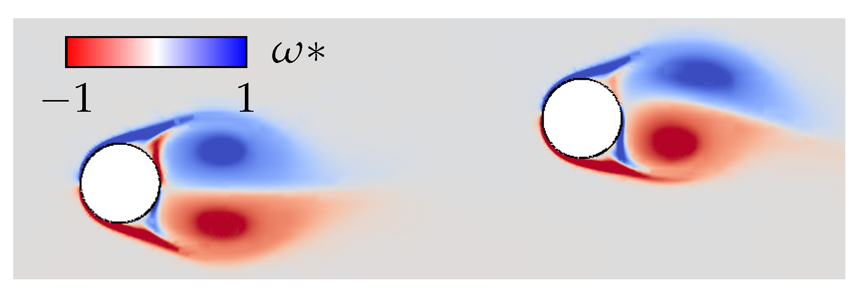
  • Basilisk [33,34,35] is a Direct Numerical Simulation (DNS) solver, which offers an accurate insight into the flow around the twines, especially if they are in tandem at low θ . For this purpose, we highlight the cross-sectional flow features impacting the drag coefficient around individual twines to trigger the shielding effect due to the various angles of attack of the net.
The materials and methods used in the present work are described in Section 2 and Section 3. The main results are reported in Section 4. The discussions, conclusions, and perspectives are reported in Section 5.
In the rest of this manuscript, the “star” symbol ( * ) denotes any dimensionless quantity, and the subscripts OF and AS, respectively, refer to quantities related to OrcaFlex and AquaSim.

2. Materials

2.1. GPGP Measured Data

There are two main necessary variables for the validation of the OF model: the towline tension and the speed through water ( u stw ) of the cleanup system. They have been continuously measured throughout the System 002 GPGP campaign, from August 2021 until December 2022, and more recently, during the GPGP campaigns of systems larger than System 002.
To measure the towline tension, a Running Line Monitor (Figure 2) is installed on each towing line. The tension is measured every second, and it is transmitted and registered to a computer on board the vessel.
These measurements were post-processed in the following manner:
  • The mean tension was calculated for periods of 3 h, for each of the towing lines. The sum of the mean values for each towline provides the combined towline tension, which is the variable to be validated in the present work.
  • The error associated with the combined towline tension was calculated. Taking the mean tension for a specific time period introduces an error because the true mean value, for a specific metocean condition, can be anywhere between the extreme values of the dynamic response. Therefore, the difference between the calculated mean and the maximum tension for the 3 h period was taken as the associated error.
  • The RLM has a high accuracy, typically between 0.5% and 2.0% of the measured load. The associated error described in the previous point is typically higher than the error associated with each instant measurement.
Regarding the speed through water ( u stw ) measurements, two main sources were considered:
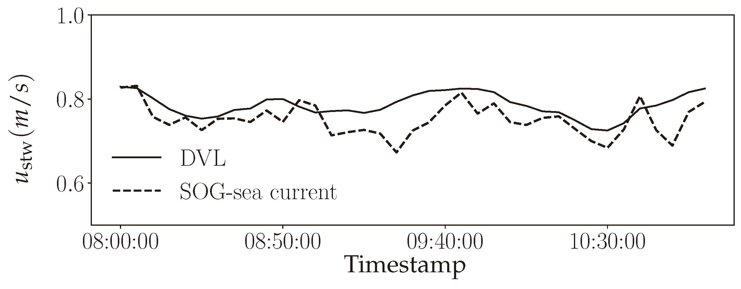
  • A Doppler Velocity Logger (DVL) supplies the u stw of the vessel, which is registered on a computer on board the vessel.
  • The Speed Over Ground (SOG) of the vessel combined with the sea surface current velocity estimation, from the X-band radar of the vessel.
The measurements produced by both sources were compared over a specific amount of time, normally corresponding to three hours of test or normal operation. If the measurements are similar, then u stw is deemed consistent, and the average between the two values is calculated and used in the validation. Figure 3 is an illustration showing this consistency between the two sources.
The error associated with the speed through water measurement is calculated in the following manner:
  • The DVL on the vessels has an accuracy of 1.5%.
  • Since two sources of data are considered to calculate the average value, an error of half the difference between the two measured values is introduced.
  • Finally, the maximum between the previous two errors is taken as the speed-through-water-associated error.
Since the OF simulations to be used in the validation process are run in the no-waves condition, the GPGP measurements must correspond to low wave conditions for comparison purposes. Based on the data gathered during the GPGP expeditions, the significant wave height range was set as H s [ 1 : 2 ] m with periods T s > 12 s, which are considered appropriate for the validation. Further details on the comparison between the OF results and GPGP data are presented in Section 3.4.

2.2. OrcaFlex

Prior to real testing or operation in the GPGP, we used OrcaFlex [29] for the dynamic analysis of System 002. Morison’s equation for the calculation of the wave loads on fixed vertical cylinders involves two force components: the fluid acceleration as the fluid inertia force and the fluid velocity as the drag force. It reads:
f O F = m f C M , OF * d u d t + 1 2 ρ f C D , OF * A | u | u
where ρ f , m f , u , C D , OF * , C M , OF * , A, and f O F , respectively, represent the density of the fluid, the mass of fluid displaced by the body, the fluid velocity relative to the Earth, the drag coefficient for the body, the inertia coefficient for the body, the drag area, and the total force on the object. In the case of a moving body, the equation reads:
f O F = m f C M , OF * d u d t C A , OF * d v b d t + 1 2 ρ f C D , OF * A | u r | u r
where C A , OF * , v b , and u r , respectively, denote the added mass coefficient for the body, the velocity of the body relative to the Earth, and the fluid velocity relative to the body. The second term is the OrcaFlex drag force ( f D , OF ).
Three components of the drag force are considered ( f D x , OF , f D y , OF , and f D z , OF ). The first two are normal to the considered line or slender cylinders. The third component is tangential. These local coordinate directions are depicted in Figure 4.
The equations applied in OrcaFlex for each of the components are the following [29]:
f D x , OF = 1 2 ρ f C D x , OF * d s l s u x | u n |
f D y , OF = 1 2 ρ f C D y , OF * d s l s u y | u n |
f D z , OF = 1 2 ρ f π C D z , OF * d s l s u z | u z |
where u n is the normal component of the fluid velocity relative to the line and u z is the axial component, d s is the diameter of the slender cylinder, l s is the length of the slender cylinder, d s l s is the normal drag area, π d s l s is the axial drag area, C D x , OF * , and C D y , OF * are the normal drag coefficients and C D z , OF * = C D , OF , a * and are the axial or tangential drag coefficient.

2.3. AquaSim

AquaSim is an FEA software for the simulation and analysis of structures exposed in the marine environment subjected to loads such as current, waves, wind, impulse loads, displacements, and other operational loads. The hydrodynamic force in AquaSim is based on the work of Berstad et al. [36].
In AquaSim, a net is the sum of twines and the total force on the net is the sum of the forces of every twine (twine-by-twine approach). If a twine is considered as a circular cylinder of diameter d t and length l t , the force for steady flow acting on the cylinder is expressed as [30]:
f D , A S = 1 2 ρ f C D , cyl * d t l t | u stw | u stw
where C D , cyl * is the drag coefficient for cross flow to a circular cylinder and u stw is the speed through water.
Considering an ideal knot-less mesh, as shown in Figure 5, the conservation of momentum indicates that, in the presence of a flow perpendicular to the net, the fluid velocity must increase. From that fact, a new drag coefficient, named C D , mem * [36], is derived and expressed as a function of C D , cyl * as follows:
C D , mem * = C D , cyl * l y l z 2 ( l y d t ) ( l z d t ) 2
Then, introducing the definition of net solidity as S n * = A e / A t o t , where A e is the netting projected area and A t o t is the total area of the net, the following relation can be deduced:
C D , mem * = C D , cyl * 1 1 S n * 2 3
with
S n * = d t l y + d t l z
Finally, the effect of fluid velocity reaching the net at an arbitrary angle is incorporated into the equation as an updated drag coefficient C D , mem * , based on the angle of attack of the mesh to the flow θ (cf. Equation (10)). This accounts for the so-called shadow or shielding effect. That is the effect an upstream twine wake has on a downstream twine (Figure 6).
C D , mem * = C D , mem * l y sin θ K * d t 1.5
where K * is proposed to be 2.4, according to the findings of Berstad et al. [36].

2.4. Basilisk

The investigation of moving rigid bodies immersed in a fluid is quite abundant in the literature along with the numerous methods tackling this kind of problem, as seen in the reviews of Wachs [37], Wu and Yang [38], Uhlmann et al. [39]. In this study, we used Basilisk, which is an open-source software providing a set of solvers based on a tree data structure. It is able to solve numerous initial-boundary-value problems. The work of Selçuk et al. [40] in Basilisk allowed us to use the Distributed Lagrange Multiplier/Fictitious Domain method (DLM/FD) originally introduced by Glowinski et al. [41,42], Patankar et al. [43], Glowinski et al. [44]. In their work, Selçuk et al. [40] showed the details of the method and its numerical implementation on the dynamic quadtree/octree grid of Basilisk to tackle the problem of immersed bodies in a fluid flow. The principle of the DLM/FD formulation consists of enforcing the rigid body motion on the immersed body domain within an Eulerian grid as a constraint and treats the body boundary and its volume as an object under solid body motion. In fact, Lagrangian points are distributed not only on the boundary, but in the volume occupied by the rigid body as well.
We briefly recall the general DLM/FD formulation for generalized freely moving bodies. It is worth mentioning that, when the bodies are fixed, their velocities are equal to zero, simplifying the conservation equations. Let Ω define a domain of R d , d < 2 , 3 > and Ω its boundary. Then, let N t * be the number of twines B i ( t ) ( i [ 1 : N t * ] ) that Ω is filled with. For the sake of simplicity, N t * is considered to be equal to 1. Dirichlet boundary conditions are set on Ω for the fluid velocity field. Dimensionless variables are defined using the set of the following variables: d t for length, u stw for velocity, t c * = d t / u stw for the convective time scale, ρ f u stw 2 for pressure, and ρ f u stw 2 / d t for the rigid-body motion Lagrange multiplier; ρ f denotes the fluid density. The combined conservation equations that govern both the fluid and the solid (if there is motion) are written as follows:
  • Continuity equation:
    · u * = 0 , over Ω .
  • Combined momentum equations:
    u * t * + u * · u * = p * + 1 R e t * 2 u * λ * over Ω ,
    ( ρ r * 1 ) V b * d v b * d t F r * g g B ( t ) λ * d x * = 0 , over B ( t ) ,
    I b * d ω * d t * + ω * × I b * · ω * + j ( F c ) j * × R j * + B ( t ) ( λ * × r * ) · d x * = 0 , over B ( t ) ,
    u * ( v b * + ω * × r * ) = 0 , over B ( t ) ,
where u * stands for the fluid velocity vector, p * the pressure, λ * the distributed Lagrange multiplier vector, r * the position vector with respect to body gravity center, I b * the body inertia tensor, R * the vector between the body gravity center and the contact point for eventual contact (but not the case in this study), V b * the body volume, M * the body mass, g * the gravity acceleration, ρ r * = ρ b / ρ f the density ratio, and g * the gravity acceleration magnitude. The twine Reynolds number R e t is defined as R e t * = ρ f u stw d t μ f , and the Froude number F r * is defined as F r * = g d t u stw 2 . The full details of this method are reported in Selçuk et al. [40], Wachs [45], Wachs et al. [46].
Using the aforementioned method, the hydrodynamic force about the ith body center of mass can be computed as:
f i * = B i ( t ) σ * · n d S *
where, σ * and n are, respectively, the stress tensor, which is the summation of the Lagrange multipliers of the rigid body, and the outward-oriented unit normal vector to B i . Hence, the total force acting on all the twines is i N t * f i * . In this study, the main focus was the drag force (therefore, the drag coefficient). As the total force is the summation of the individual forces acting on each twine, it is legitimate to consider the twine’s projected area for the calculation of the drag coefficients. For each twine, the dimensional drag force is written as:
f D , CFD i = 1 2 ρ f C D , CFD i * A i | u stw | u stw ,
then the average drag coefficients of the net can be defined as:
C D , CFD * ˜ = 2 i = 0 N t * f D , CFD i ρ f A u stw 2
where A i is the cross-sectional area of the ith twine. Since A i remains constant for all twines, we can write A = i = 0 N t * A i .
In this study, the drag coefficients were projected onto the net intrinsic reference frame (Section 3.5 ). Its axes’ unit vectors are defined as normal and axial (respectively, n and a ).
C D , CFD , n * ˜ = 2 i = 0 N t * f D , CFD , n i ρ f A u stw 2 C D , CFD , a * ˜ = 2 i = 0 N t * f D , CFD , a i ρ f A u stw 2

3. Method

3.1. Overview of the Method

Describing the method implies describing the inputs, outputs, interfaces, and processes necessary to achieve the objective of validating the OF model. An effective way to present this is through the flowchart in Figure 7, which can be further clarified with the following points:
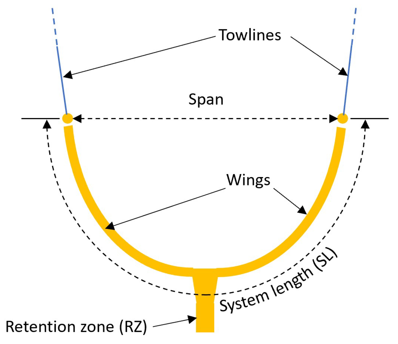
  • The variable to validate is the combined towline tension, defined as the sum of the tensions in each towline, for various speeds through water u stw . The span is the distance between the wing’s extremities as depicted in Figure 8. The figure also shows the System Length ( S L ), towlines, wings, and Retention Zone (RZ). The System Ratio ( S R * ) is defined as the ratio between the span and the system length ( S R * = s p a n / S L ).
    Three span values are considered as shown in Table 1 for System 002’s length equal to 800 m:
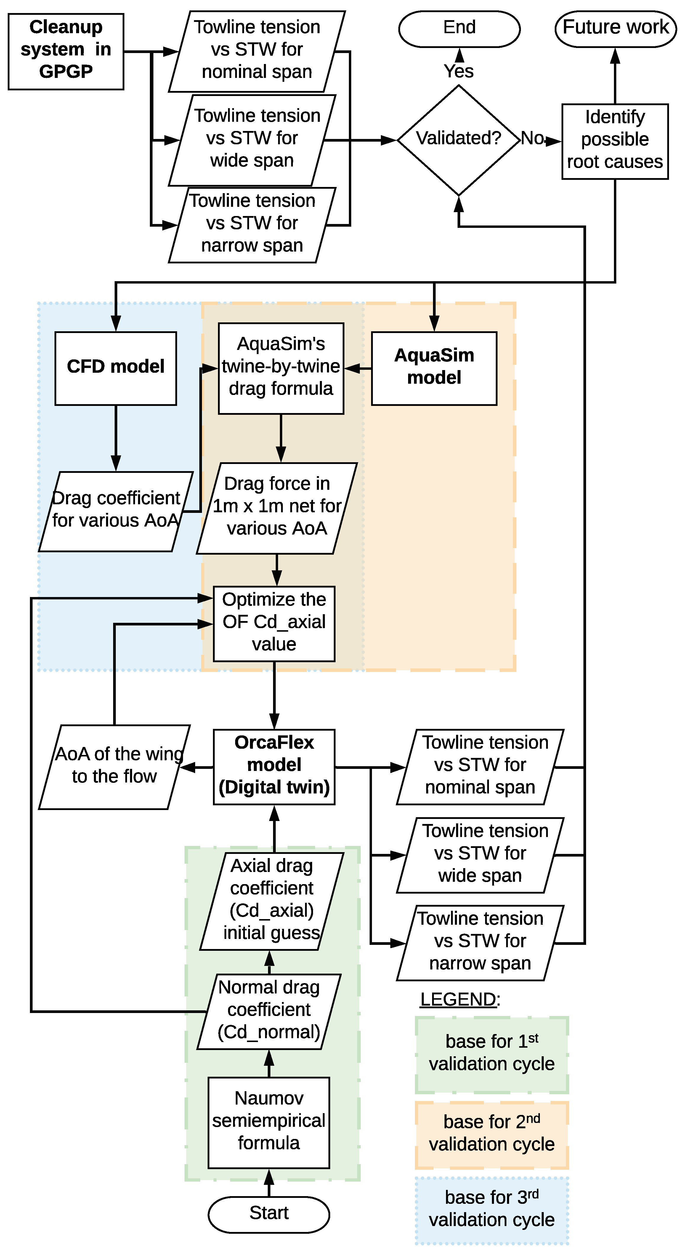
  • The OF model validation was performed in three cycles:
    • First cycle: Simulation based on the initial estimation of the OF axial drag coefficient C D , OF , a * . This step is detailed in Section 3.2.
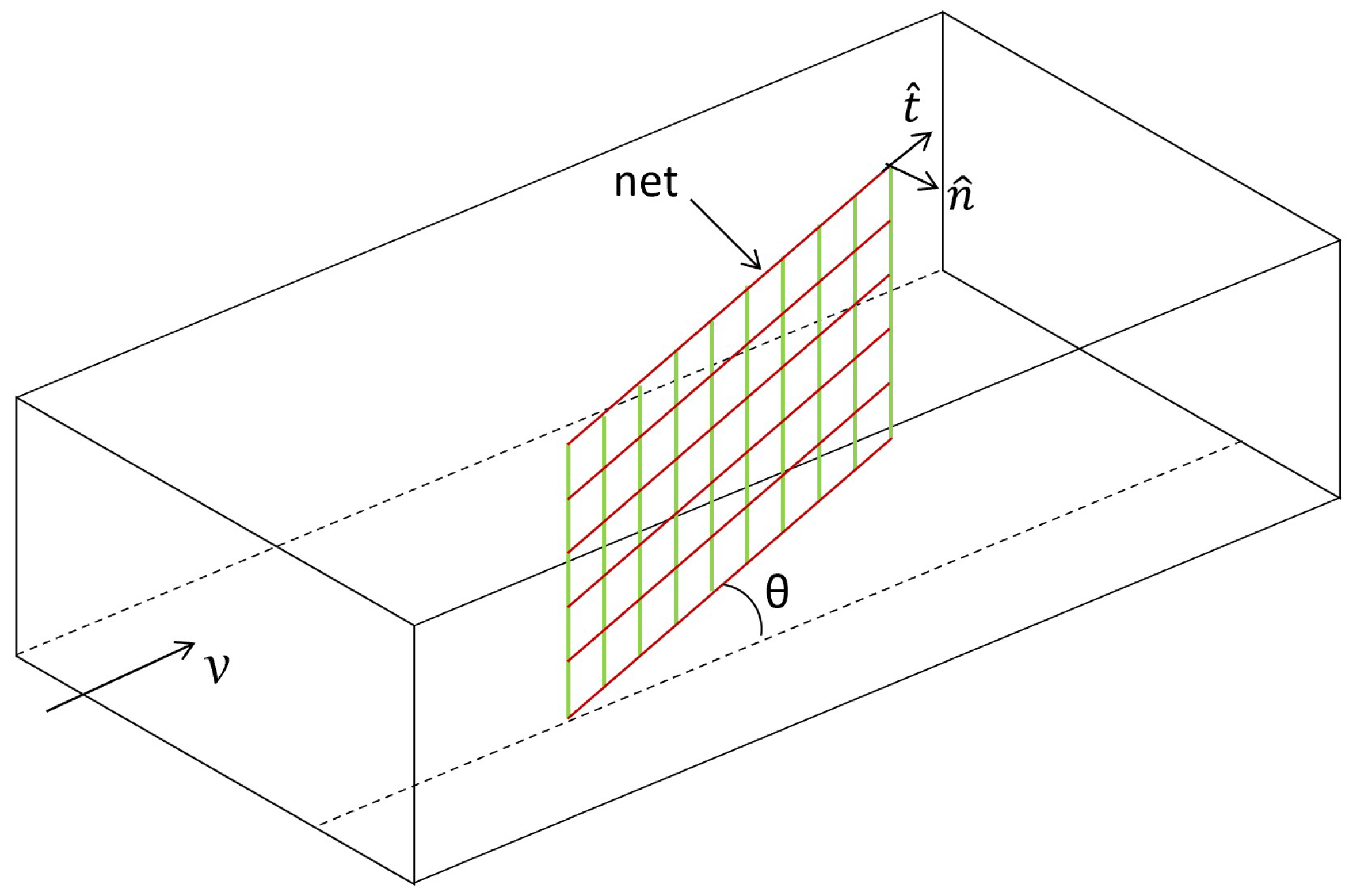
    • Second cycle: Triggered by discrepancies between the model and the GPGP data, especially for a narrow span, we used the AS model of a 1 m × 1 m piece of the system’s net at multiple θ . Then, the difference between the drag forces on a 1 m × 1 m section of the net from OrcaFlex and AquaSim was calculated and written as:
      Δ f D = f D , OF f D , AS
      Then, the Root Mean Square (RMS) of the set of differences for a group of θ , corresponding to a certain span, can be calculated:
      R M S = 1 N θ * j = 1 N θ * | Δ f D | j 2
      where N θ * is the total number of angles of attack for the optimization case. The optimization objective is to obtain the C D , OF , a * value that produces the minimum RMS for the specific optimization case. In that way, the OF drag force will be close to the AS drag force. With this optimization, the accuracy of a twine-by-twine calculation and the shielding effect can be included in OF, leading to more-accurate load estimations. Further details about the OrcaFlex modeling are seen in Section 3.2.
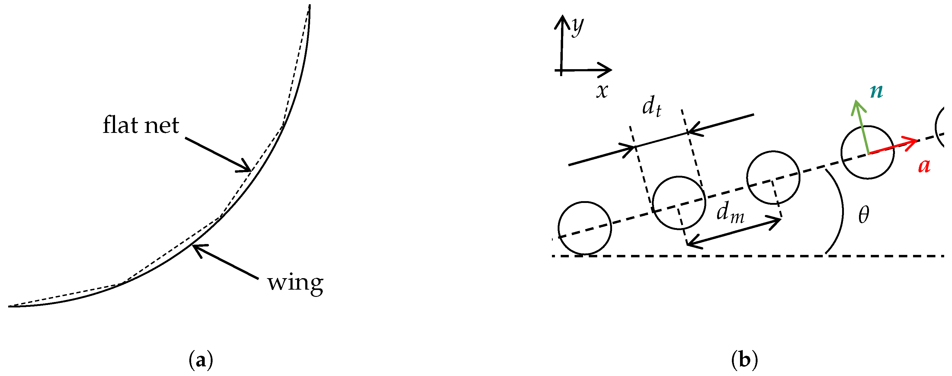
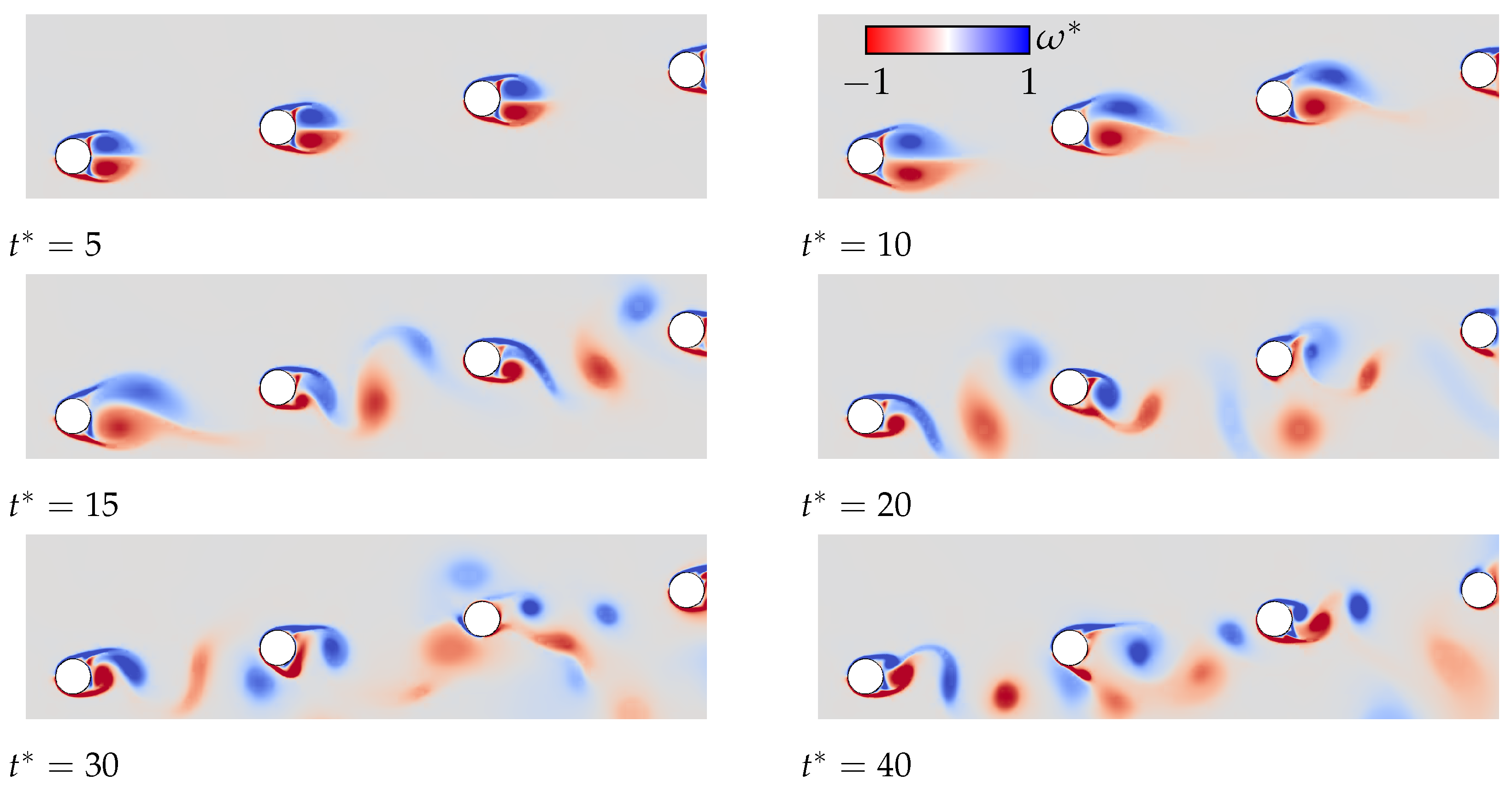
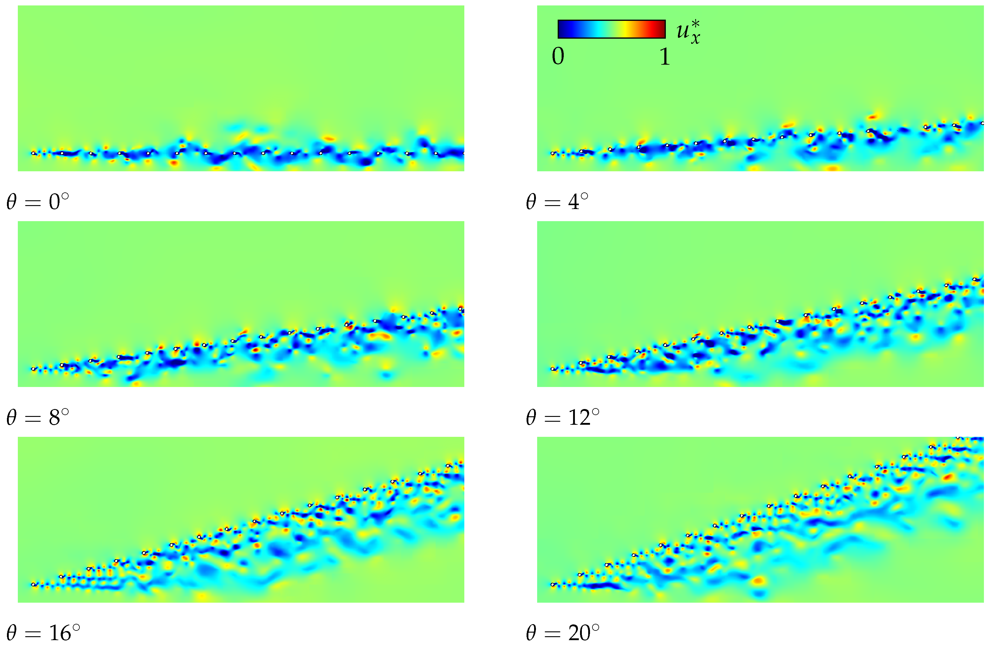
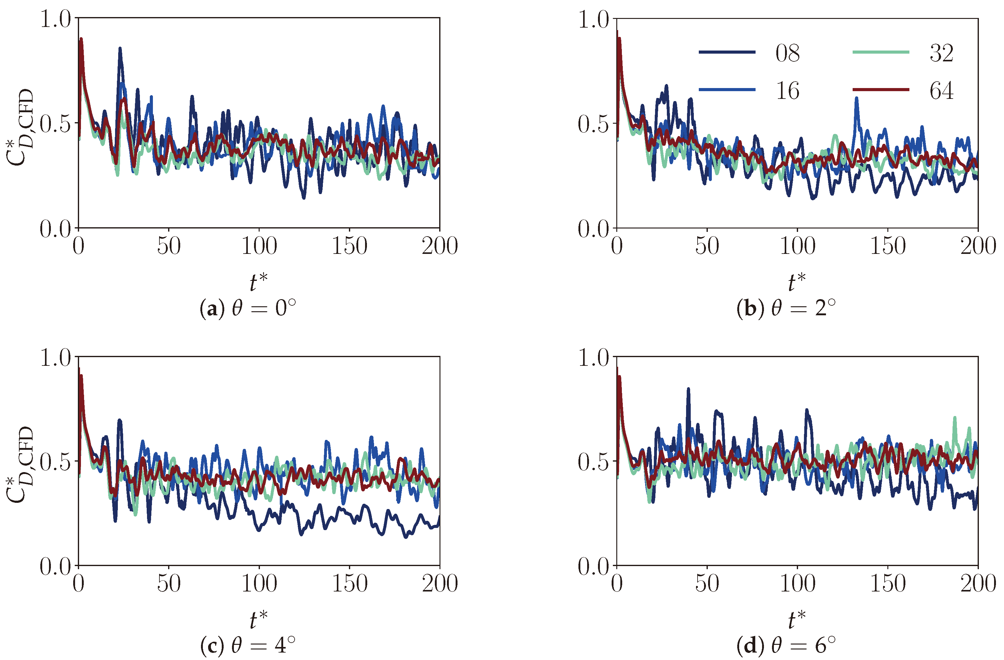
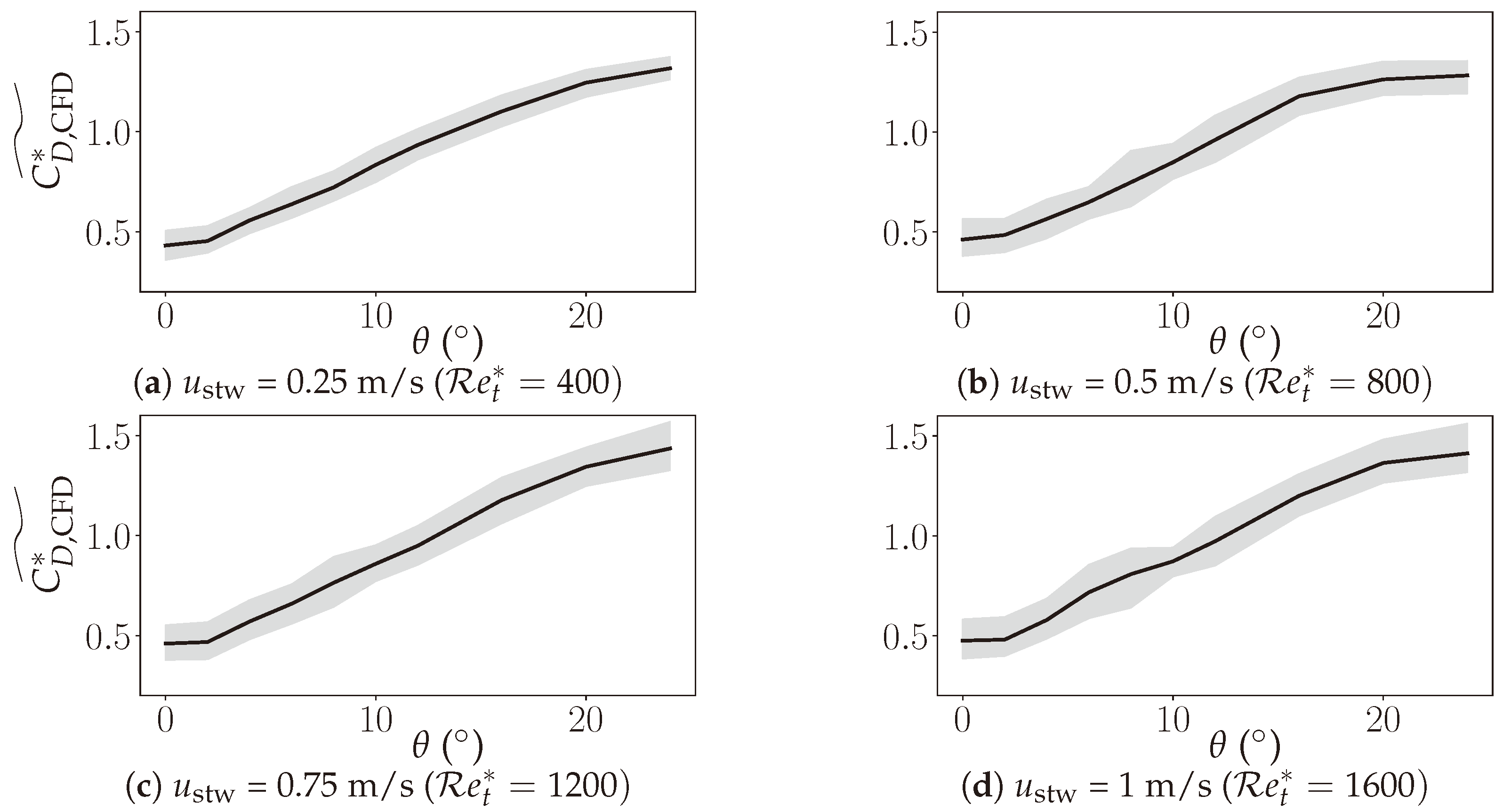
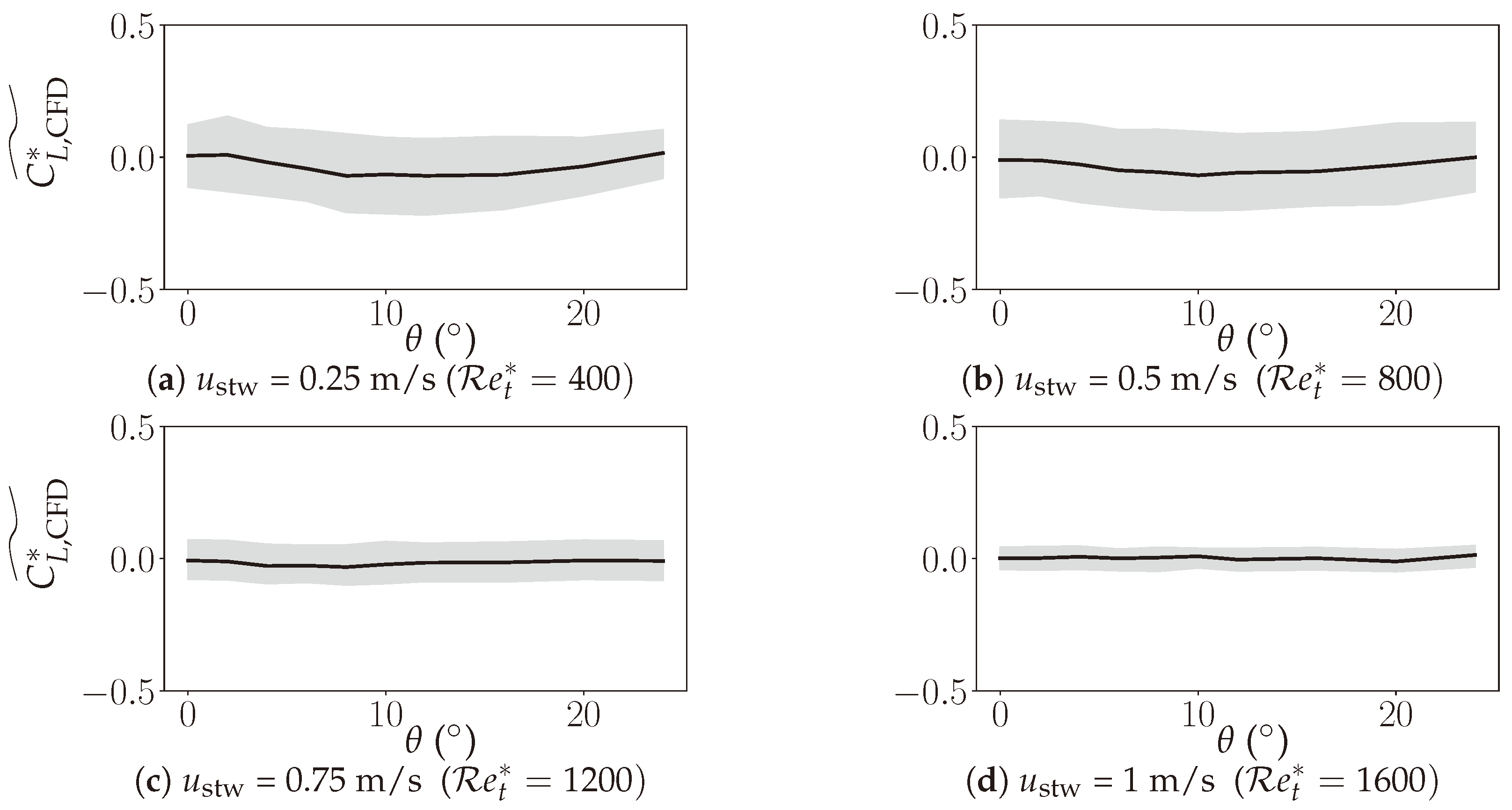
    • Third cycle: Triggered by the necessity to verify the AS results, using a CFD model, a two dimensional piece of the net was simulated for various θ to quantify the effect of the vortex shedding on the twines in tandem on the average drag coefficient. This gives a piecewise definition of the average drag coefficients of the net. They are given as a function of u stw and θ and used in the AS drag force Equation (28), replacing the AS drag coefficients. Then, the same optimization (Equations (20) and (21)) can be carried out one more time.

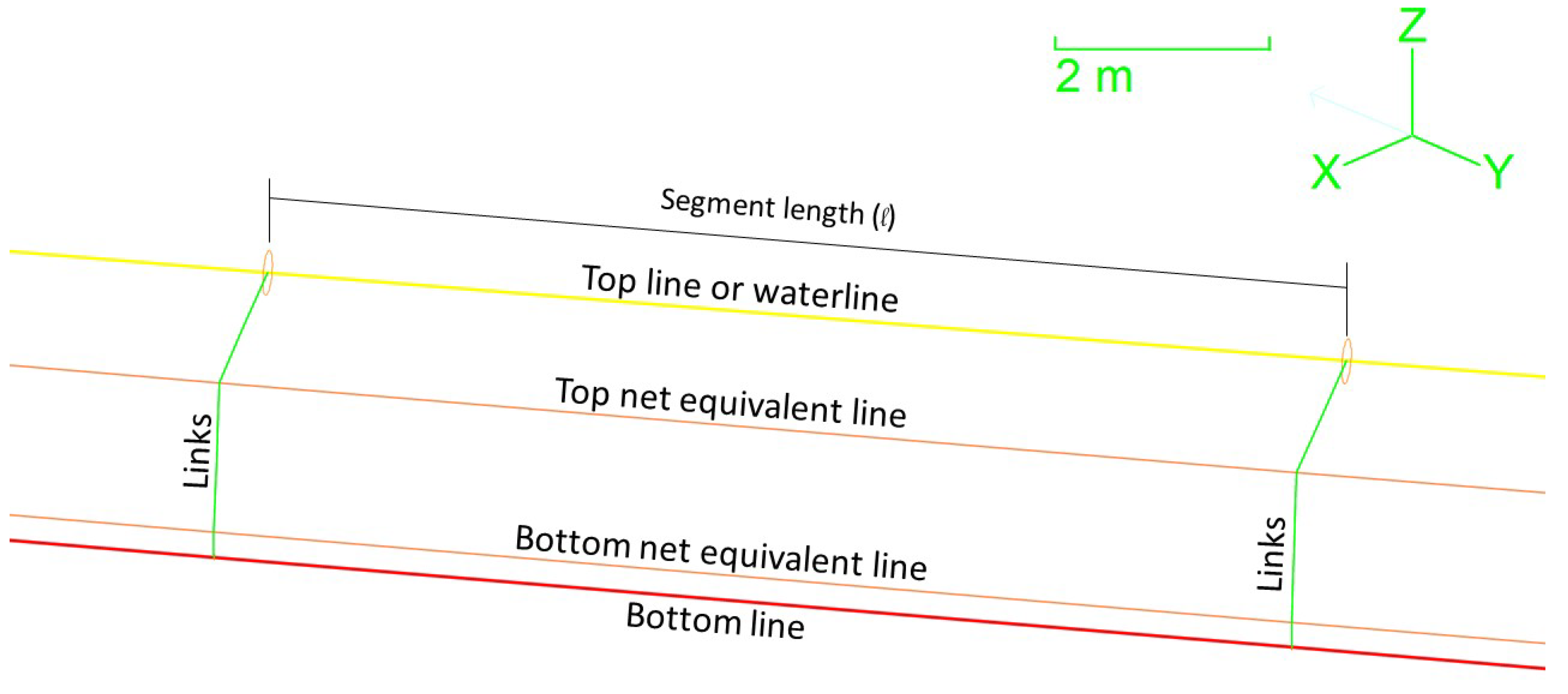
3.2. OrcaFlex Drag Force Calculation

In this section, the question of how to apply the OF calculation capability, described in Section 2.2 to a fishing net, is answered. The used approach is to convert the net into equivalent horizontal cylinders or lines called net equivalent lines, running along the system wings, segmented based on a user-defined slender length ( l s ), and vertically connected by links. Figure 9 presents a section of the wings modeled in OrcaFlex. The drag contribution of each segment is added along the wing to obtain the total drag force on that line. Since the wing underwater shape also influences the drag, it is necessary at least to have two drag equivalent lines vertically distributed to obtain a better representation of the real-world data (cf. the two orange lines in Figure 9).
The normal drag coefficients of the net equivalent lines ( C D x , OF * and C D y , OF * ) were assumed equal to the normal drag coefficient derived from the semi-empirical formula proposed by Naumov et al. [11], which reads:
C D , n * = 19.4 2 ξ * R e t * 0.36 , R e t * < 400 ξ * , 9.3 2 ξ * R e t * 0.22 , 400 ξ * R e t * < R e c * , 1.41 + 1.7 ξ * , R e t * R e c * .
with
ξ * = d t s m i = 0 n | h i | defined in R n , n = 2
R e c * = 2 ξ * 9.33 1.41 + 1.7 ξ * 4.63
where d t , d m , h i , and R e c * , respectively, denote the twine diameter, the mesh size or twine distance, the directional hanging ratios, and the critical Reynolds number related to the transition to a non-linear drag formulation.
The OF axial drag coefficient ( C D , OF , a * = C D z , OF * ) was initially approximated as 1 / ( 3 π ) of the normal drag coefficient, as this approximation is conservative. As an example, in the work of Berstad et al. [36], the tangential or axial drag coefficient was estimated to be 1–2% of the normal drag coefficient.
The OF model had the following three important limitations that triggered the need for a second validation cycle. They also determined the optimization method for the OF axial drag coefficient:
  • Due to the way the net is modeled, since potential flow and one-way coupling were considered, there was no option to directly include or capture what is called the shielding effect between the twines of a submerged net. In contrast, the drag calculation in the software AquaSim and Basilisk does include this effect.
  • Due to the way the net was modeled, it was not possible to calculate the drag twine-by-twine and actually differentiate between horizontal and vertical twines. In contrast, the drag calculation in the software AquaSim does include this option.
  • The effect of the underwater cross-section shape of the net has on the drag force was not included in the model. Both OF normal drag coefficients were considered equal. That is, C D x , OF * = C D y , OF * = C D , OF , n * = C D , n * . This effect can be included by considering the torsion of the drag equivalent line, but that considerably increases the computation time.
Finally, the OF drag force f D , OF for a 1 m × 1 m piece of plain net was constructed considering the angle of attack θ , the speed through water u stw , the net solidity S n * , the  C D , OF , n * , C D , OF , a * , as well as the normal ( n ^ ) and axial/tangential ( t ^ ) directions. It reads:
f D , OF = ( f D · n ^ ) 2 + ( f D · t ^ ) 2
In kilogram-force:
f D , OF = ρ f S n * 2 g C D , OF , n * u stw 2 sin 2 θ 2 + π C D , OF , a * u stw 2 cos 2 θ 2

3.3. AquaSim Drag Force Calculation

Using AquaSim, the drag force on a 1 m × 1 m piece of flat net can be derived as follows: (i) the number of meshes N m * in 1 m 2 of a net with l y = l z = L (Figure 5) is given by N m * = 1 L 2 ; (ii) the drag force f D , AS is constructed considering the angle of attack θ , the twine diameter d t , C D , mem * (Equation (8)), C D , mem * (Equation (10)), and the speed through water u stw . Each term of the equation is linked through colors to either horizontal or vertical twines, as depicted in Figure 10. The force reads:
Jmse 11 01943 i010
In kilogram-force:
Jmse 11 01943 i011
C D , a , t * is the axial drag coefficient of a twine, and it was taken as 1.3 % of C D , cyl * , which is between 1% and 2%, as suggested by Berstad et al. [36], and C D , cyl * = 1 for all the range of Reynolds numbers experienced by the twine of the cleanup system’s net.
Equation (28) was used during the last two validation cycles to calculate the drag force acting on a 1 m by 1 m plane net. This force was then used to optimize the OF axial drag coefficient.

3.4. Comparing GPGP Data with Simulation Results

As mentioned in Section 2.1, H s [ 1 : 2 ] m was used to select the GPGP data. In that range, there is a considerable amount of measurements available and the wave height is relatively close to the no-wave condition imposed in the simulations.
In spite of the relatively low waves, towing the system in waves produces an increase in the mean towline tension. That increase varies as a function of u stw and the metocean conditions. In order to compare the GPGP data with the simulation results, it is necessary to quantify that increase for different speeds and sea states. The quantification of the increase in the mean towline tension in waves was based on OF simulations. We computed wave factors using the results from several System 002 simulations in head sea and nominal span. The wave factor is the ratio between the towline force in waves and the towline force in no waves. They are presented in Table 2 for various u stw and various sea states. From this table, it can be deduced that the wave factors decrease with increasing u stw , and they increase with increasing sea state. Since System 002 normally operates at u stw [ 0.75 : 1.0 ] m/s, it makes sense to focus on that velocity range during the validation procedure. It also makes sense to validate for year-average conditions, that means for annual p50 conditions. Then, a wave factor of 1.15 (reading from the p50 row and 0.75 m/s column) can be used to multiply the combined towline tension estimated by OrcaFlex. That leads to a valid and conservative comparison between the simulation and real-world data.

3.5. Problem Setup for CFD Model

The meshing of the net is defined such that the ratio between the twine distance and the twine diameter d m / d t is equal to 5.882. The system is towed by two vessels with targeted u stw equivalent to Reynolds number R e t * [ 400 : 1600 ] . We modeled our system as a collection of flat nets consisting of a row of circular cylinders in two dimensions (Figure 11b). This will help us quantify the cross-sectional shielding effect on the twine drag coefficients. The modeling approach is exhibited in Figure 11a. The approach consisted of establishing a piecewise definition of the whole submerged net. These segments have an angle of attack θ relative to the flow direction. Therefore, θ varies according to the location of the piecewise plane net on the wings, and it is estimated as θ [ 0 : 90 ] ° . Since it is impossible to obtain accurate flow features around the full-scale net, this decomposition approach appears to be a good alternative for our needs.

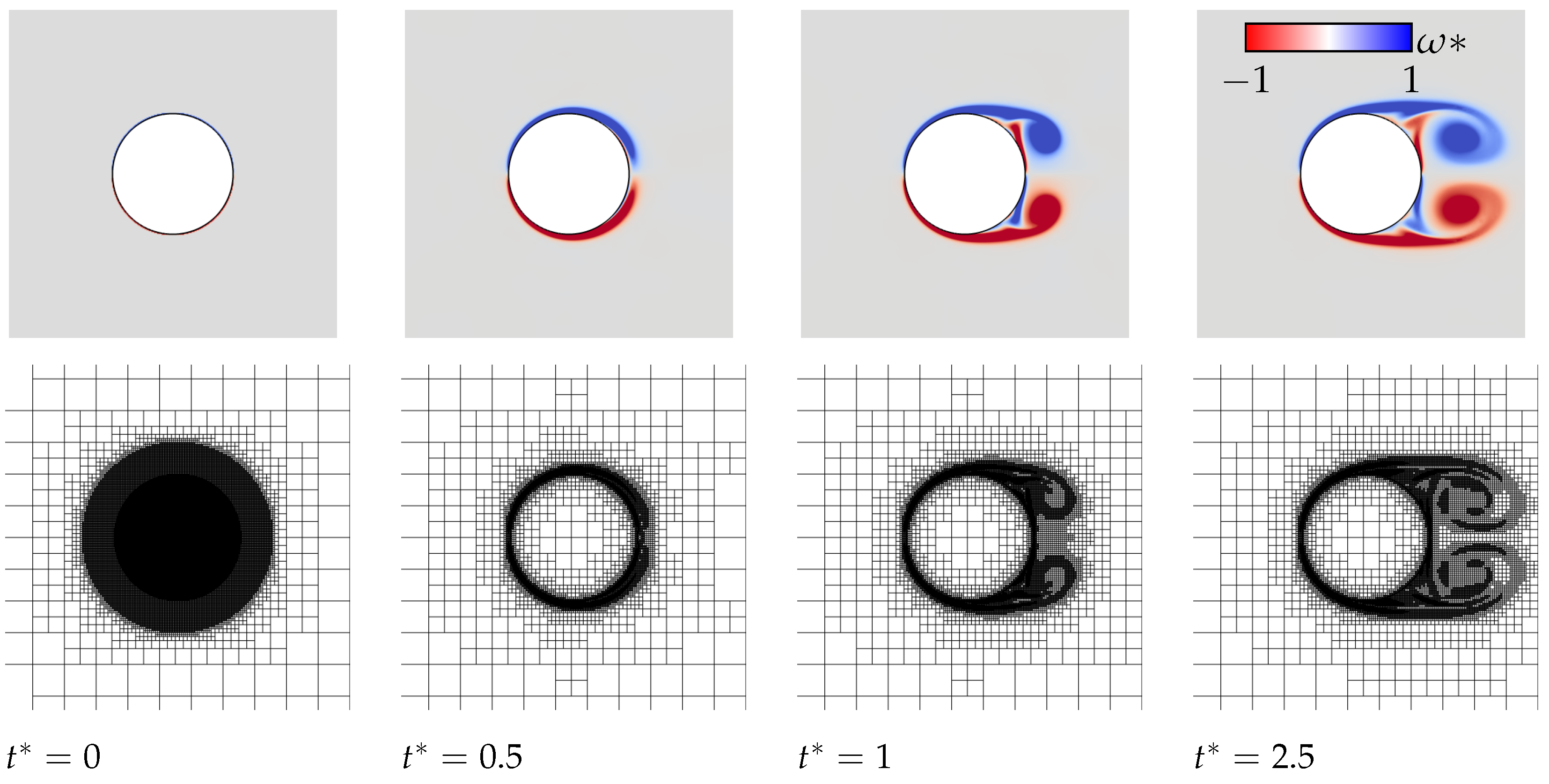
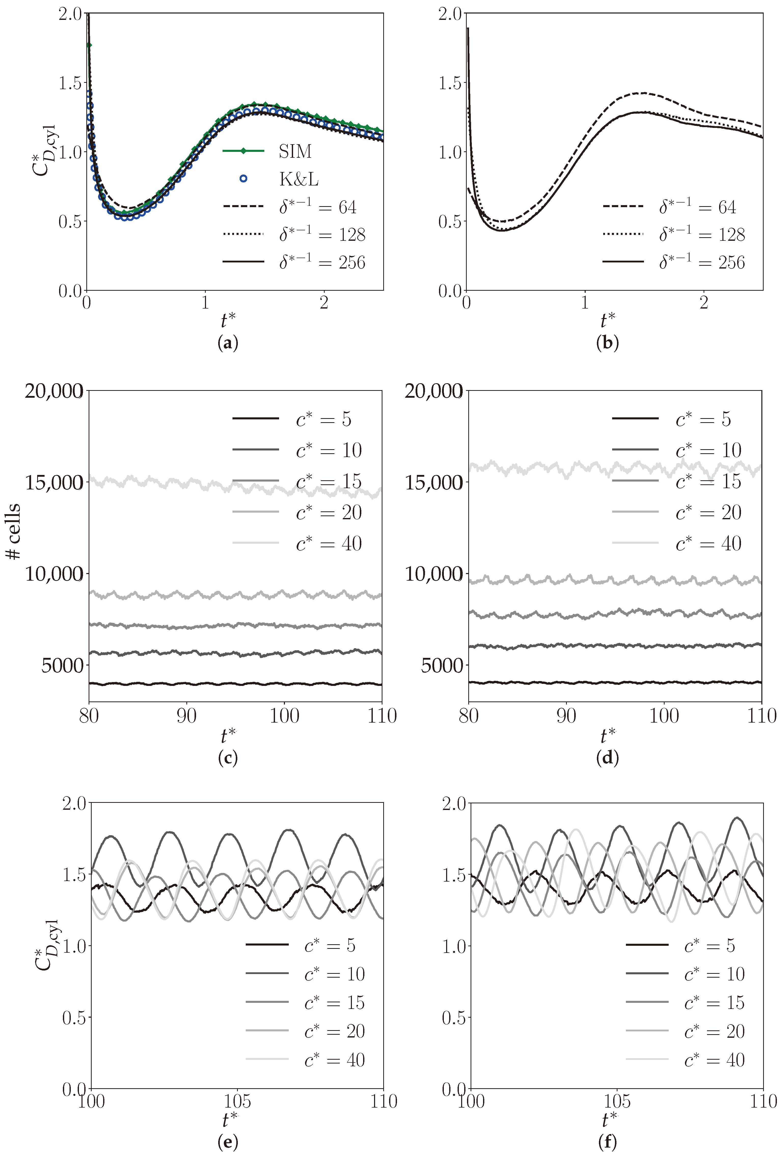
3.5.1. Space Convergence on Flow Past a Circular Cylinder

The accuracy of the present method was assessed in this section. In fact, the spatial key parameters of the AMR features are the maximum level of refinement M * giving the smallest grid size defined as Δ = L 0 / 2 M * , where L 0 is the domain size and the refining criteria c * such that the threshold u stw / c * is necessary to locally refine the grid. In the case of this study, we chose to refine the grid based on the change of the velocity fields. Naturally, in the following, we define the number of discretisation points along a twine diameter as δ * 1 = d t / Δ and the dimensionless time as t * = u stw t / d t . Furthermore, the test consisted of computing the drag coefficient for a single circular body immersed in a constantly moving fluid. The impulsively started flow past a unit-diameter circular cylinder problem is a good candidate to help us in choosing the right numerical parameters to solve the problem of complex boundary layer separation over the circular cylinder. As outlined in Figure 12, the case was based on the experiments of Bouard and Coutanceau [47], and noteworthy early numerical simulations were the works of Koumoutsakos and Leonard [48] and Mohaghegh and Udaykumar [49], hereafter, respectively, referred to as K&L and SIM. In Figure 13a, we show a space convergence with Basilisk on the chosen test case. Additionally, Figure 13c depicts the necessary effort to compute the drag force according to the refinement criteria c * . Finally, we show in Figure 13e the effect for the refinement criteria c on the drag coefficient.
Hereafter, it is clear to us to use a set of ( δ * 1 , c * ) = ( 128 , 20 ) to sufficiently capture the unsteady behavior of the flow behind the cylinder width a relatively modest effort.

3.5.2. Convergence on the Drag Coefficient of Multiple Twines in Tandem at Various Angles of Attack

In this section, we quantified the effect of multiple twines in tandem on the drag coefficient at a low angle of attack. As a matter of fact, the shielding effects are only observed at low angles of attack. An example of the illustration of this effect is depicted in Figure 14 and Figure 15 for R e t * = 1000 . It can be seen that only the leading twine conserves the vortex-shedding pattern, which is responsible for the unsteady separation of the flow, whereas the following twines exhibit broken patterns due to the wake of their respective preceding twine. Therefore, the goal of this section was to show the number of twines N t * for which the average drag coefficient is no longer changing.
In Figure 16, we compare the time history of the instantaneous averaged drag coefficient computed as in Equation (18), but relative to the x-axis. It shows a very clear dependence on the number of twines N t * . For small N t * , the drag coefficient is underestimated by more than 50%. For our following analysis, it is obvious that we considered only N t * 32 . Since the difference between N t * = 32 and N t * = 64 is acceptable and for a relatively modest computational effort, we chose N t * = 32 .
In order to improve our DT, we extracted the drag and lift correlations as seen in Figure 17 and Figure 18. By analyzing these correlations, we can gain a better understanding of the behavior of an object in a fluid medium and how factors such as the angle of attack and velocity affect the drag and lift. It is worth noting that the drag coefficient is almost three-times higher for high angles of attack compared to very low angles of attack. This underscores the importance of considering a wide range of angles of attack when modeling the behavior of a net in a fluid medium and highlights the need for accurate drag and lift correlations in order to create more-precise predictions.

4. Results

4.1. First Validation Cycle
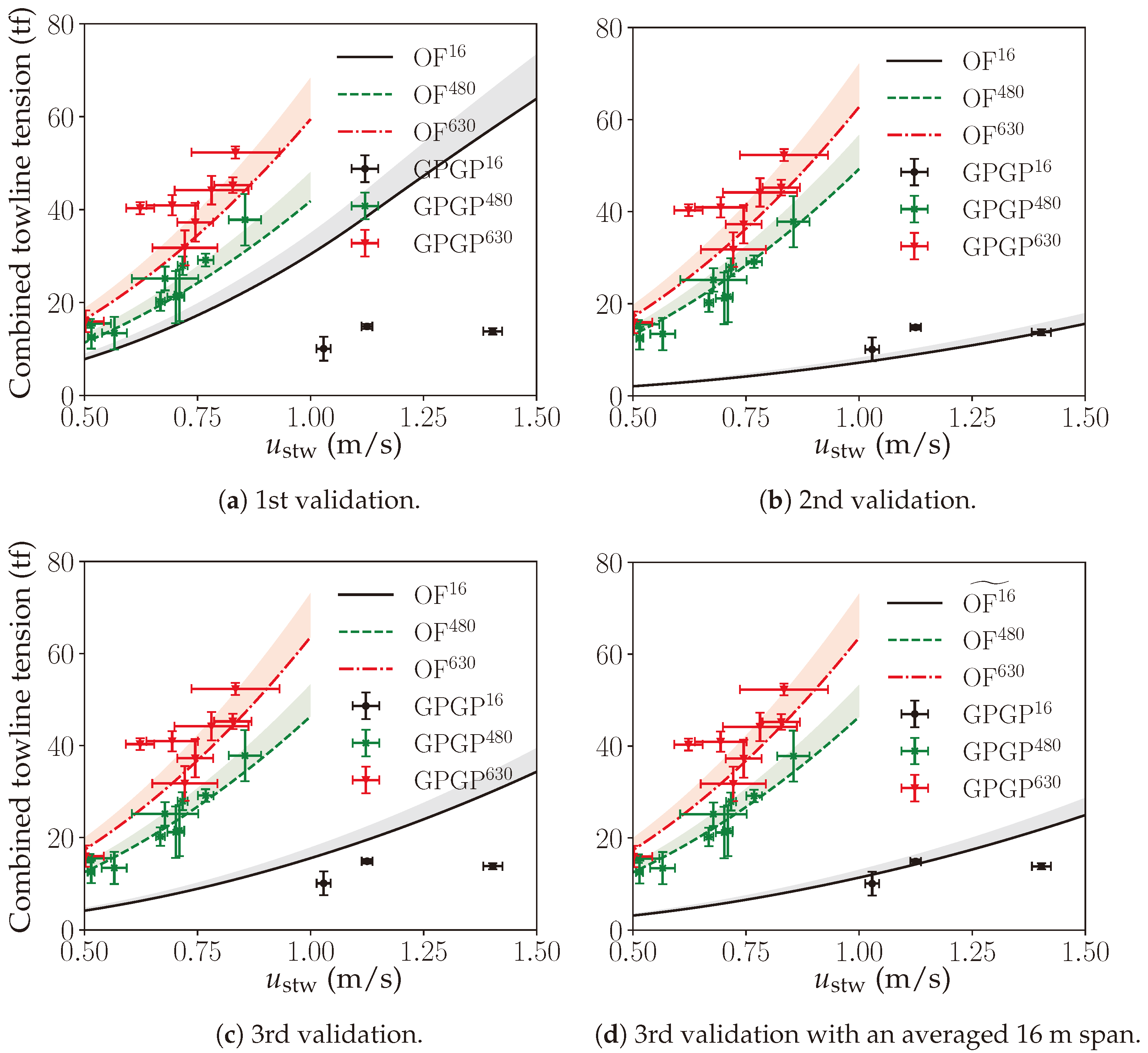
The first validation cycle was based on the drag coefficients derived from the semi-empirical formula of Naumov et al. [11], as shown in Figure 7. These coefficients were applied to the OF DT of System 002. u stw was varied from 0.25 m/s to 1.0m/s in no-wave conditions and with a simulation time t = 2500 s to reach a steady span.
Based on Figure 19a and the comparison criteria given in Section 3.4, a validation criterion can be defined. Focusing on the u stw ranging between 0.75 m/s and 1.0 m/s for nominal and wide spans and between 0.75 m/s and 1.5 m/s for a narrow span, if the data points fall close to or inside the 15% increase area, the simulated curve can be considered as validated. A deviation percentage was also quantified. Considering this, the following findings can be identified:
  • The axial drag coefficient C D , OF , a * led to a DT estimation larger than the measured data in the narrow span. Specifically, the average deviation between the 15% increase area and real-world data was about 276%. The main phenomenon that was not captured by OF in this case was the shielding effect (cf. Section 2.3 for an explanation on this effect).
  • The axial drag coefficient C D , OF , a produced a 15% area that was close to the GPGP data points for the nominal span. Nevertheless, the majority of the data points were still outside of the area, and the computed mean deviation was about −3% (minus sign meaning an underestimation of the ground truth). The expectation was that the second and third validation cycle curves will comply even better with the validation criteria. The reason behind this expectation is that C D , OF , a was not optimized for the angles of attack to the flow and the twine-by-twine calculation had not been included yet.
  • The axial drag coefficient C D , OF , a produced a 15% area that was close to the GPGP data points for a wide span. Even some data points were inside the area, and the calculated mean deviation was just 1%. That means that the OF model might be considered as validated at this cycle for a wide span. Nevertheless, the expectation was that the 2nd and 3rd validation cycle curves would comply with the validation criteria in a more-conservative manner, following the same reasoning as for the nominal span.

4.2. Second Validation Cycle

As is shown in the flowchart of Figure 7, the second validation cycle was mainly based on an optimization process of the OF axial drag coefficient ( C D , OF , a ) with the objective of imitating the AS-calculated drag force over a 1m × 1m net, for multiple θ . Therefore, the present section is divided in two subsections: (i) Section 4.2.1 deals with the optimization cases, which means to define, per span type, which θ are relevant; (ii) Section 4.2.2 presents the findings derived from the second cycle’s results depicted in Figure 19b.

4.2.1. Optimization Cases

The optimization cases depend on the angle of attack θ assumed by the wings for different system spans. Therefore, defining the case requires an analysis of the OF simulation results for each span presented in Table 1. Since there is symmetry, only the results for one wing were considered.
The distribution of the angles of attack along the wing, for the narrow span, is presented in Figure 20a for two values of u stw . As can be seen, with  u stw = 0.5 m/s, the angles of attack were concentrated between 0 ° and 2 ° . That trend strengthened if the speed was increased to 0.75 m/s. Therefore, for a narrow span, C D , OF , a should be optimized for θ 2 ° .
The distribution of the angles of attack for the nominal span is presented in Figure 20b for two values of u stw . In this case, for both values of u stw , about 50% of the angles were between 20 ° and 30 ° and the rest were between 30 ° and 85 ° . According to the CFD results and AS calculation, no major shielding effect was expected for θ > 24 ° . Therefore, the shielding effect was limited for the nominal span, meaning that C D , OF , a can be optimized for angles between 30 ° and 90 ° in order to cover 50% of the angles and give more importance to the higher drag forces close to 90 ° .
The distribution of the angles of attack for the wide span are presented in Figure 20c for two values of u stw . As can be deduced, for both u stw values, about 50% of the angles were between 30 ° and 45 ° , whereas the other 50% were between 45 ° and 90 ° . From the CFD simulations and AS calculation, no major shielding effect was expected for θ > 24 ° . Therefore, the shielding effect was very limited for a wide span. Therefore,  C D , OF , a can be optimized for θ [ 45 : 90 ] ° in order to cover 50% of the angles and give more importance to the higher drag forces close to 90 ° .
The optimization cases are summarized in Table 3:

4.2.2. Findings Based on Second validation Cycle Results

Once the C D , OF , a * was optimized based on the AS drag calculation, the OF model was updated, and the results from these simulations were plotted together with GPGP measurements (data points) and the 15% increase in the mean load, explained in Section 3.4 (colored area above the curves), to produce Figure 19b. Based on the latter and using the same validation criteria as for the first validation cycle, the following findings can be identified:
  • The optimized C D , OF , a * for a narrow span was definitely more accurate than the first cycle value. That demonstrated the influence of the shielding effect on the drag coefficients. Nevertheless, the 15% increase area was still below the data around u stw = 1.0 m/s and u stw = 1.1 m/s. This means that the DT was slightly underestimating for narrow span. The mean deviation in this case was −10%.
  • The optimized C D , OF , a * also produced a more-accurate and more-conservative nominal span curve, in comparison with the first cycle, since all data points between u stw = 0.75 m/s and 1.0 m/s were inside the 15% increase area or below the curve. Having points below the curve might mean that the second cycle curve was slightly overestimating the towline tension for nominal span. Indeed, the mean deviation was about 14%.
  • The optimized C D , OF , a * led to the majority of the data points falling inside the 15% increase area. The mean deviation was computed as 6%. Then, the DT can be considered as validated and sufficiently overestimating for a wide span. This also means that the AS calculation was enough to calibrate the OF axial drag coefficient C D , OF , a * and to obtain a proper estimation of the towline tension in a wide span.

4.3. Third Validation Cycle

Once the C D , OF , a * was optimized based on the CFD results, the OF model was updated, and the results of these simulations were plotted together with GPGP data and the 15% increase in the mean load, explained in Section 3.4, to produce Figure 19c. Based on the latter and using the same validation criteria as for the 1st and 2nd validation cycles, the following findings can be drawn:
  • The optimized C D , OF , a * for a narrow span produced more-accurate results than the first cycle. The results were also more conservative than the second cycle ones. Nevertheless, the curve in no waves was above all points. This means that the DT was overestimating, specifically by a mean deviation of 97%. This overestimation might be due to a missing phenomenon or effect related to the flexibility of the net and the shape it adopts under water. In spite of the overestimation and from an engineering perspective, the 3rd cycle curve was preferred over the 2nd cycle curve. A better option, again from an engineering perspective and to obtain more-accurate results, is to average both curves. That averaged result is plotted in Figure 19d. In terms of validation, it can be said that the DT had not been validated yet for the narrow span. The validation for narrow span depends on future studies. Nevertheless, the validation effort brought the 276% deviation of the 1st cycle to about a −10% deviation after the 2nd cycle and to about 97% after the 3rd cycle. If the averaging option was applied, the combined deviation was about 43%.
  • The optimized C D , OF , a * produced a more-accurate nominal span curve than for the second cycle, since almost all GPGP data points were inside the 15% increase area curve. The mean deviation in this case was just 7%. This also means that the DT was validated for a nominal span.
  • The optimized C D , OF , a led to the majority of the GPGP data points falling inside the 15% increase area, and the mean deviation was calculated to be 8%. Then, the DT at the third cycle can be considered as validated for a wide span. Since the wide span curve was considered as validated already on the second cycle, this result also means that the CFD calculation verified the AS calculation for a wide span.

4.4. Calibrated Drag Coefficients for System 002

The results presented in Figure 19 are a consequence of the optimization of the OF axial drag coefficient ( C D , OF , a * ) for different span lengths. Those coefficients, in turn, are a consequence of the mesh cross flow drag coefficients ( C D , mem * ), calculated with the AquaSim Equation (10) (2nd validation cycle) and estimated by the CFD model (3rd validation cycle). Therefore, it is important to tabulate and analyze these coefficients.
Table 4 includes the mesh cross flow drag coefficients ( C D , mem * ) for the 2nd and 3rd cycles, for different angles of attack.
It is clear that the drag coefficients of the second validation cycle exhibited a sharp reduction until 0.0 with decreasing θ . In contrast, the coefficients estimated by the CFD model followed a less-steep reduction, and in parallel flow, the value was larger than 0.0. This difference explains the deviation between the 2nd and 3rd validation cycle towline tension curves. As an example to quantify the difference, the 3rd cycle drag coefficient was 9.5-times larger than the second cycle drag coefficient at an angle of attack of 2°. In other words, the CFD model provided an estimate of the shielding effect that was very different from the estimate given by AquaSim Equation (10).
Another relevant remark is that the C D , mem * values at 90° were lower than the value of 1.9623 obtained from Naumov semi-empirical Formula (22). This is logical since, in both, the AquaSim formulation and CFD model, the twine is modeled as a cylinder. In Naumov’s case, the twine is a real one moving through water. The results presented in Figure 19 indicate that the Naumov value seems closer to the real-world data and keeping it as the OF normal drag coefficient ( C D , OF , n * ) led to accurate results.
Table 5 presents the OrcaFlex recommended axial drag coefficients for System 002’s net and for u stw > 0.5 m/s.
For a narrow span, the axial drag coefficient decreased from 0.208 in the first cycle to 0.01 in the second cycle and increased to 0.082 in the third cycle. This is consistent with the differences in the mesh cross flow drag coefficient ( C D , mem * ) shown in Table 4. Taking the average of the second and third cycles yielded an axial drag coefficient of 0.046, which is a 78% decrease relative to the first cycle.
For the nominal span, the axial drag coefficient increased from 0.208 in the first cycle to 0.332 in the second cycle and to 0.285 in the third cycle. This is consistent with the differences in the mesh cross flow drag coefficient ( C D , mem * ) shown in Table 4 for an angle of attack of 30°. The 0.285 coefficient represents a 37% increase relative to the first cycle.
For the wide span, the axial drag coefficient increased from 0.208 in the first cycle to 0.301 in the second cycle and further increased to 0.324 in the third cycle, which is a 56% increase relative to the first cycle.

4.5. Boundaries for the Application of the Results

Several results were presented in the previous sections. Nevertheless, it is not clear which boundaries define the scope of application of these results. Moreover, it is neither clear how these results can be applied to other systems, either larger cleaning systems or other netting systems operating in different sectors.
These boundaries are described in the diagram presented in Figure 21. As can be seen, the core (green and orange color) is the scope related to System 002 and the present study, highlighting the inputs, results, project phase, and sector of application. Some of these findings can be readily utilized for new netting systems (colored in orange) when opting for OrcaFlex as the software to build the DT. These encompass the optimization methodology and the software’s constraints and potential opportunities. In contrast, the remaining portion of the results (colored in green) requires modification, recalculation, or re-modeling to align with the requirements of the new netting system.
There are two important clarifications. First, Cleanup System 0X means any future cleanup system (e.g., System 03). Second, the present study considered three discrete system ratios, but in reality, the validation needs to be performed for a larger range of S R * .

5. Discussion and Conclusions

Section 4 was dedicated to present the results from the validation process. In this section, these results are seen from the perspective of the main assumptions and the previous studies, in order to generate conclusions and recommended future studies. Since the validation process consisted of three cycles, it is logical to organize this section making reference to these three cycles.
The main assumption for the first cycle was that the normal drag coefficient obtained from the study of Naumov et al. [11], together with an axial drag coefficient approximation, should be sufficient to accurately model the drag force of the net for different system spans in OrcaFlex. The results in Section 4.1 show that, as the system’s span increased, the net started to resemble the net in perpendicular flow of the experiment carried out by Naumov et al. [11]. That led to a towline tension curve that accurately followed the GPGP data trend for a wide span. In contrast, when the system’s net was experiencing parallel flow almost all along its length (i.e., narrow span), the towline tension considerably deviated from reality. That was due to the fact that an axial drag coefficient magnitude of C D , OF , a * = 1 3 π C D , OF , n * applied all along the wings is too high, in comparison with the reduced drag coefficient as a consequence of the shielding effect when θ < 24 ° . The nominal span result, which slightly underestimated reality, can be explained by comparing Equations (26) and (28). The AS equation includes the term f vert · t ^ , which represents the tangential component of the drag on the vertical twines in cross flow. In the OF model, that term cannot be included in the calculation with the cross flow drag coefficient, but only with the parallel (axial) flow drag coefficient, which is lower in magnitude, leading to the underestimation.
In summary, after the first cycle, it was found that the Naumov semi-empirical formula [11] was sufficient to accurately estimate the drag force of the ocean system’s net in wide span with a mean deviation of just 1%, which, from another perspective, might be considered as lacking the desired minimum overestimation. Besides this, the first two limitations of the OF model, listed in Section 3.2, explain the deviation from reality of the drag force estimation for nominal and narrow spans.
Moving forward to the second cycle, there were three key assumptions. First, by using the AS calculation, defined by Berstad et al. [36], the large deviation between the towline tension curve for a narrow span and the GPGP data should be reduced, because the shielding effect is taken into account. Second, by using the AS calculation, the underestimation of the towline tension for nominal span should be reduced, since the twine-by-twine drag calculation is included. Third, the AS calculation can be reproduced in the OF model by optimizing the OF axial drag coefficient for the θ assumed by the system’s wings in different spans.
The second cycle’s results (Section 4.2) demonstrated that the first assumption is valid. Actually, applying the AS formula for the reduced drag coefficient (Equation (8)) corrected the narrow span curve from 276% deviation from GPGP data to about −10% deviation. The second assumption is also valid, and in fact, the towline tension curve for nominal span moved from a slightly underestimating position to a slightly overestimating position (from a −3% deviation to a 14% deviation), which is preferable. The third assumption was proven to be true since it was demonstrated that the OF axial drag coefficient optimization method, presented in Section 3.1, improved the estimation of the DT, and it can be consistently repeated for different system spans.
Finally, it was assumed that, by developing the third validation cycle, the towline estimation should be improved even further. Besides this, a second assumption was that the CFD model should capture the physics of the problem, including the shielding effect, and therefore, it could be used to verify the AS drag coefficients and the AS shielding effect formula proposed by Berstad et al. [36].
Following the third validation cycle (Section 4.3), the first assumption was proven correct for a nominal span and a wide span. The CFD model produced drag coefficients in cross flow that were close to the AS values, but they led to an even more-accurate towline tension in the nominal span, in comparison with the second validation cycle’s results (the mean deviation improved from 14% to 7%). For the narrow span, the drag coefficients derived from the CFD model generated an overestimation of the towline tension of about 97%. Therefore, the first assumption was not validated for the narrow span, but improvement is expected after including physical phenomena currently missing in the CFD model, for example the net’s flexibility. The outcome was similar for the second assumption. The AS calculation method was verified for nominal and wide spans, but the AS formula in Equation (8) reduced the drag coefficient for low θ more than what was estimated by the CFD model and actually slightly more than what the GPGP data indicated. Therefore, further investigation is necessary to verify what is actually happening in the narrow span. In the meantime, and only for engineering and design purposes, the average between the 2nd and 3rd towline tension curves can be used to obtain results in the narrow span that deviate on average 43% from reality.
There were also general assumptions, meaning that they applied to all three validation cycles. For example, it was assumed that the drag force over other wing components (fenders, ropes, chains, etc.) was correctly modeled in OrcaFlex and/or that the drag force produced by these components was small in comparison with the net’s drag. Although neither of these assumptions have been proven yet, the accuracy of the results indicates that both of them are probably true.
A second general assumption is related to the OF and the CFD models. It was assumed that modeling the system’s net as explained in Section 3.2 and Section 3.5 was sufficient to obtain accurate results for the towline tension. In light of the results from the validation process, presented in Figure 19a–c, this assumption was proven correct.
A third general assumption is related to the CFD model and AS calculation and the quantification of the shielding effect. It was expected that the estimated reduction of the cross-flow drag coefficient when moving from perpendicular flow to parallel flow would be similar for both AS and CFD. The 2D DNS with Basilisk, in nominal operation with u stw = 0.75 m/s and Reynolds number around of 1000, estimated a reduction of about 70%. AS estimated a reduction of 100%. The consequence of that difference was a 3rd cycle towline tension curve in the narrow span that doubled the 2nd cycle’s curve (cf. Figure 19b,c). Since none of these curves were enough to validate the CFD model or the AS calculation, a twofold future investigation needs to be developed. On the one hand, the CFD model needs to be analyzed and improved adding possible missing physics. As an example, the facts that the net is flexible and that it deforms in parallel flow have not been considered yet. On the other hand, the assumptions and supporting data behind the AS formula need to be investigated and validated.
Based on the previous discussion, two types of implications or conclusions can be established. The first type comprises the conclusions directly related to the objective of the present study. The second type comprises conclusions that align with a wider perspective or context and that have an impact on the research or industry sectors.

5.1. Objective-Related Conclusions

Based on the results presented in Section 4, the discussion reported in Section 5, and considering that the main objective of the present study was to improve the accuracy of the hydrodynamic loads’ (mainly the drag force) estimation of the DT, the following objective-related conclusions can be established:
  • The accuracy of the DT on the towline tension estimation of the ocean cleanup System 002 in wide span ( S R * 0.8 ) was improved from having several GPGP data outside of the 15% increase area. Moreover, the DT for the wide span was validated against the GPGP data, with sufficient overestimation (respectively, 6% and 8% mean deviations), at the 2nd and 3rd validation cycles.
  • The accuracy of the DT estimation of the towline tension of the cleanup System 002 in the nominal span ( S R * 0.6 ) was improved from from having most of the GPGP data outside of the 15% increase area. Moreover, the OF model (i.e., the DT) for the nominal span was validated against the GPGP data at the third validation cycle, with a mean deviation of 7%.
  • The accuracy of the DT on the towline tension estimation of the ocean cleanup System 002 in the narrow span ( S R * 0.02) was improved. An initial deviation of 276% with respect to the GPGP data was reduced in the 2nd cycle to −10% and in the 3rd cycle to 97%. In spite of the OF model for the narrow span having not been validated yet and that more GPGP data points are required for a more-robust validation, a combined deviation of 43% can be considered for engineering and design purposes, once the average of the 2nd and 3rd cycle curves is taken.
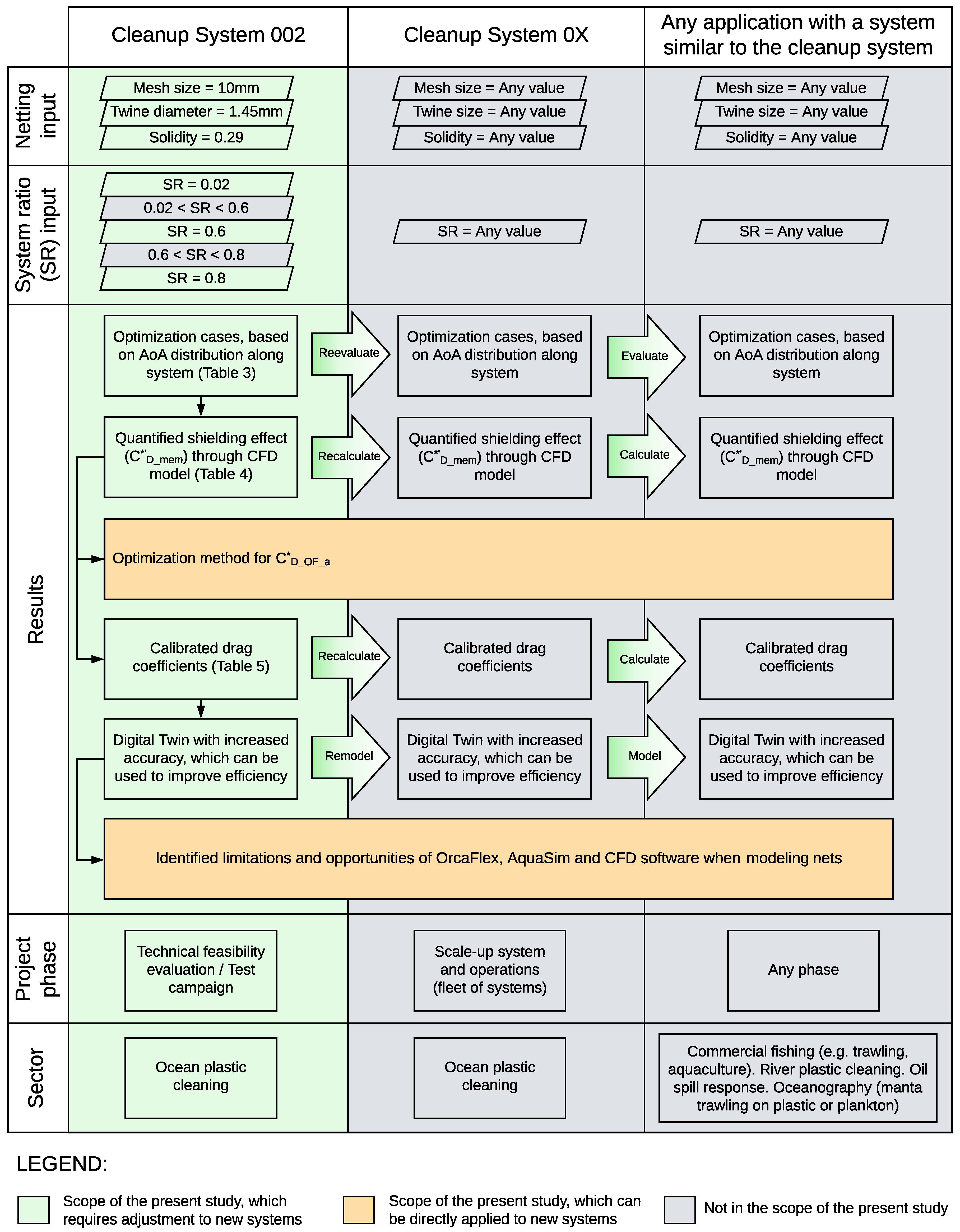
  • The results obtained for System 002 can be either directly applied to System 03 and future systems, if the netting and system ratio inputs are the same, or easily reevaluated, recalculated, and remodeled in case the inputs are different (cf. Figure 21). Therefore, considering the same input, System 03 DT can be also considered as validated for wide and nominal spans.
  • The previous conclusions have important implications for The Ocean Cleanup development. First, the DT of System 002 and System 03, provided that the latter has the same net and SR characteristics of the former, can be used to improve the efficiency of the operations. As an example, the towing configuration can be dynamically optimized through a trip, to sail with a large span when the plastic area density is high (plastic hot-spots) and in a short span in low-density areas. The under-designing and over-designing of the cleanup system were minimized, further reducing capital expenditure, but also operational expenditure by limiting the case of under-designed systems experiencing failures during operation. The maneuverability of the system can also be improved. As an example, the effect of optimizing the netting sizes can be accurately estimated. That will also improve efficiency since the system will reach and be swept through plastic hot-spots faster. Ultimately, all these improvements will bring the KPIs to values that are below the projected targets.

5.2. Wide-Ranging Conclusions

Based on the results presented in Section 4, the discussion reported in Section 5, and focusing on the implications or impacts on a context wider than the present study, the following wide perspective conclusions can be established:
  • The quantification of the shielding effect is considerably different if it is performed with the AS calculation or with the CFD model. On top of that, neither the Basilisk model nor AS produce a towline tension curve that accurately fits the GPGP data for a narrow span. Therefore, both calculation methods should be investigated to find the source of the difference.
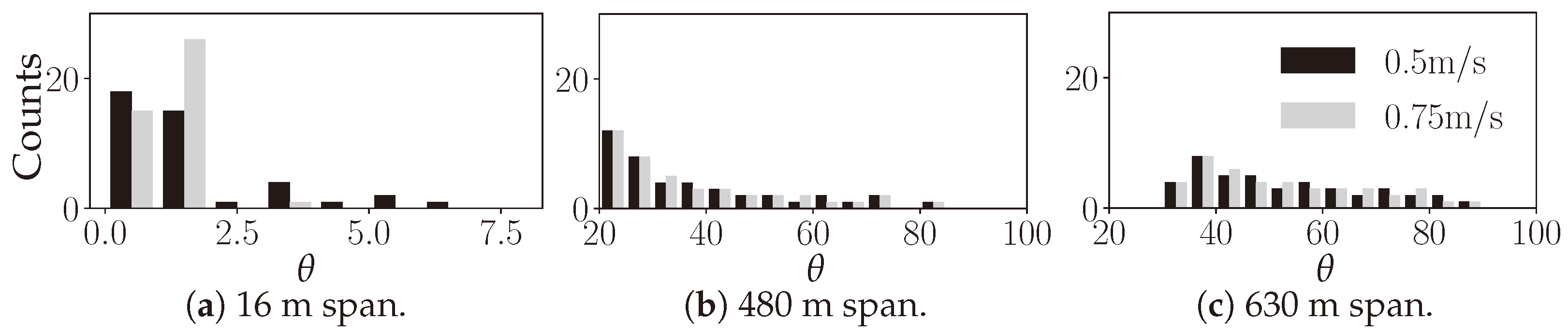
  • Through the validation cycles, it was demonstrated that the semi-empirical formula of Naumov et al. [11] can be used to obtain drag coefficients that produce sufficiently accurate towline tension estimations when the net being towed experiences a flow that is close to perpendicular along most of its length. In terms of θ , 50% or more of the angles found along the length are distributed between 45° and 90°. The same applies for the AS calculation and the CFD-derived drag coefficients. Furthermore, additional (future) GPGP data for a narrow span need to be included to strengthen the validation.
  • Through the validation cycles, it was demonstrated that the AS drag calculation was consistent with the CFD drag calculation until approximately θ 24 ° . Below that angle, which is close to parallel flow, AS seemed to underestimate the real drag and the CFD model seemed to overestimate it. Therefore, a more in-depth investigation of AS Equation (8) and of the CFD model to identify missing physical phenomena is required. In that way, the root causes of the respective deviations can be identified.
  • As clearly depicted in the schematic of Figure 21, it is possible to adapt and apply the results of the present study to different systems, utilized in sectors ranging from river plastic cleaning to oceanography, through to trawling, aquaculture, oil spill response, and marine ecology. In particular, the optimization method of the OrcaFlex drag coefficient can be directly applied to any of these applications, as well as the lessons on the limitations and opportunities of the software. That should allow running OrcaFlex simulations that produce accurate estimations on motions, loads, maneuverability, operability, survivability, and steering strategies, among others. This can be combined with the modeled data on the catch itself (plastic, fish, plankton, oil, etc.) to obtain accurate estimations on catch rates. Then, considering the invested energy or input, this would lead to efficiency estimations. Ultimately, this allows developing optimization actions to improve the efficiency of the system.
    Additionally, the present study can also be utilized by other applications or sectors as a guideline to develop the following activities:
    • To understand the hydrodynamic drag force experienced by submerged nets and the previous research related to it.
    • To validate a model using the materials, knowledge, and method presented in this study.

6. Directions of Further Research

Objectively, this work helped us to fundamentally understand the limitations of the software packages (OrcaFlex and AquaSim) that we use on our daily operations. Despite these obstacles, this research study gave us the opportunity to implement a workflow that helps us to overcome them, although we presented a relatively simple two-dimensional down-scaling approach with its limitations. With the very first version of our Digital Twin, we can now foresee research directions towards which we could improve our Digital Twin either from the numerical or from the application point of view.

6.1. Multi-Scale Numerical Approach

Through the validation cycles, it was demonstrated that the AS drag calculation was consistent with the CFD drag calculation until approximately θ 24 ° . Below that angle, which is close to parallel flow, AquaSim seemed to underestimate the real drag and the CFD model seemed to overestimate it. Therefore, a more in-depth investigation of AS Equation (27) and of the CFD model to identify missing physical phenomena is required. As such, CFD offers a very good insight into the intricacy of the interaction between the net and the surrounding fluid. We aim to model that fluid–structure interaction at multiple local levels of detail induced by the presence of twines to the macroscopic definition of the cleanup systems. Due to the flexibility of the net and its three-dimensional geometry, we will incorporate the third dimension CFD information into our future Digital Twin. We will borrow a well-known method in the field of multiphase flow to solve the behavior between a continuous fluid and a net made with bonded rigid particles. It is known as Discrete Element Method-Computational Fluid Dynamics (DEM-CFD), also known as meso-scale four-way coupled Euler–Lagrange (Anderson and Jackson [50], Kawaguchi et al. [51], Tsuji et al. [52], Esteghamatian et al. [53]). The DEM solver [54,55] calculates particles’ positions, velocities, and forces based on the interactions between individual particles, taking into account factors such as friction, collision, and cohesion. When these particles are bonded, they create a fiber, and a net is just a collection of fibers, as evidenced in the studies of Kong et al. [56,57], Li et al. [58]. The formulation’s core idea involves averaging conservation equations for fluid to account for the presence of DEM particles. It includes closure terms, mainly hydrodynamic forces, to account for how these particles react with the fluid, which are fed into Newton’s equations for the particles to consider the fluid. The added value of this approach is that we can include plastic debris in the numerical environment so that we have a better insight into the efficiency of the netting of our cleanup systems.

6.2. How to Hydrodynamically Choose a Net for Our KPIs?

The KPIs stated in Section 1 are closely linked to both the twine diameter and the mesh size defining the solidity of the net (Figure 22a), which, in turn, drastically influence the total drag coefficient (Figure 22b). In essence, a large mesh size would potentially decrease the hydrodynamic loads on the cleanup system, but leave behind the plastics of small sizes, whereas a small mesh size would substantially increase our CO 2 footprint and the cost of our offshore operations.
The improvement of our Digital Twin would provide us a map of multiple “What if” scenarios when choosing the nets of our future cleanup systems. The improvement can be quantified as the size and shape of the mesh that are designed to target most (if not all) of the floating plastics combined with an optimized hydrodynamic efficiency.
Finally, as we only covered three values of the System Ratio ( S R * = 0.02 ; 0.06 ; 0.8 ), we need to assess the effect of the entire spectrum 0.02 S R * 0.9 on these KPIs. This is particularly important at a narrow span during the deployment and the recovery of the system mainly for safety reasons since our offshore crew executes them from two towing vessels. Moreover, additional (future) GPGP data for a narrow span needs to be included to strengthen the validation.

Author Contributions

Conceptualization, M.A.G.J., A.D.R. and D.J.C.; methodology, M.A.G.J., A.D.R. and D.J.C.; validation, M.A.G.J. and A.D.R.; formal analysis, M.A.G.J.; investigation, M.A.G.J. and A.D.R.; resources, M.A.G.J. and A.D.R.; data curation, M.A.G.J.; writing—original draft preparation, A.D.R.; writing—review and editing, A.D.R., M.A.G.J., B.S.-R. and D.J.C.; visualization, M.A.G.J. and A.D.R.; project administration, B.S.-R. and D.J.C.; funding acquisition, B.S.-R. and D.J.C. All authors have read and agreed to the published version of the manuscript.

Funding

This research was funded by the donors of The Ocean Cleanup.

Institutional Review Board Statement

Not applicable.

Informed Consent Statement

Not applicable.

Data Availability Statement

The raw data required to reproduce the findings in this work and the software application are available from Andriarimina Daniel Rakotonirina upon email request [email protected].

Acknowledgments

We acknowledge The Ocean Cleanup for the permission to publish this work and the offshore team of The Ocean Cleanup for the data collection.

Conflicts of Interest

The authors declare no conflict of interest. The funders had no role in the design of the study; in the collection, analyses, or interpretation of the data; in the writing of the manuscript; nor in the decision to publish the results.

References

  1. Tauti, M. The force acting on the plane net in motion through the water. Nippon Suisan Gakkaishi 1934, 3, 1–4. [Google Scholar] [CrossRef]
  2. Christensen, B. Hydrodynamic modeling of fishing nets. In Proceedings of the OCEAN 75, Okinawa, Japan, 20 July 1975–18 January 1976; pp. 484–490. [Google Scholar] [CrossRef]
  3. Berteaux, H.O. Buoy Engineering (Ocean Engineering, A Wiley Series); John Wiley and Sons: Hoboken, NJ, USA, 1976. [Google Scholar]
  4. Laws, E.; Livesey, J. Flow through screens. Annu. Rev. Fluid Mech. 1978, 10, 247–266. [Google Scholar] [CrossRef]
  5. Rudi, H.; Aarsnes, J.; Dahle, L. Environmental forces on a floating cage system, mooring considerations. In Aquaculture Engineering Technologies for the Future; Hemisphere Publishing Corporation: London, UK, 1988; pp. 97–122. [Google Scholar]
  6. Rudi, H.; Løland, G.; Furunes, L. Model Tests with Net Enclosures. Forces on and Flow through Single Nets and Cage Systems; MTC: Trondheim, Norway, 1988. [Google Scholar]
  7. Løland, G. Current Forces on and Flow through Fish Farms. Ph.D. Thesis, University of Trondheim, Trondheim, Norway, 1993. [Google Scholar]
  8. Takagi, T.; Suzuki, K.; Hiraishi, T. Modeling of net for calculation method of dynamic fishing net shape. Fish. Sci. 2002, 68, 1857–1860. [Google Scholar] [CrossRef] [PubMed]
  9. Balash, C.; Colbourne, B.; Bose, N.; Raman-Nair, W. Aquaculture net drag force and added mass. Aquac. Eng. 2009, 41, 14–21. [Google Scholar] [CrossRef]
  10. Zhao, Y.P.; Li, Y.C.; Dong, G.H.; Gui, F.K.; Teng, B. Numerical simulation of the effects of structure size ratio and mesh type on three-dimensional deformation of the fishing-net gravity cage in current. Aquac. Eng. 2007, 36, 285–301. [Google Scholar] [CrossRef]
  11. Naumov, V.; Velikanov, N.; Kikot, A.; Bojarinova, N. The hydrodynamic drag coefficient of flat netting at a cross-section flow. In Proceedings of the Contributions on the Theory of Fishing Gears and Related Marine Systems: Proceeding of the 11th International Workshop on Methods for the Development and Evaluation of Maritime Technologies, Rostock, Germany, 9–12 October 2013; Volume 8, p. 73. [Google Scholar]
  12. Zhao, Y.; Guan, C.; Bi, C.; Liu, H.; Cui, Y. Experimental investigations on hydrodynamic responses of a semi-submersible offshore fish farm in waves. J. Mar. Sci. Eng. 2019, 7, 238. [Google Scholar] [CrossRef]
  13. Cheng, H.; Li, L.; Aarsæther, K.G.; Ong, M.C. Typical hydrodynamic models for aquaculture nets: A comparative study under pure current conditions. Aquac. Eng. 2020, 90, 102070. [Google Scholar] [CrossRef]
  14. Cheng, H.; Ong, M.C.; Li, L.; Chen, H. Development of a coupling algorithm for fluid-structure interaction analysis of submerged aquaculture nets. Ocean. Eng. 2022, 243, 110208. [Google Scholar] [CrossRef]
  15. Simonsen, K.; Tsukrov, I.; Baldwin, K.; Swift, M.; Patursson, O. Modeling flow through and around a net panel using computational fluid dynamics. In Proceedings of the OCEANS 2006, Boston, MA, USA, 18–21 September 2006; pp. 1–5. [Google Scholar] [CrossRef]
  16. Zhao, Y.P.; Bi, C.W.; Dong, G.H.; Gui, F.K.; Cui, Y.; Guan, C.T.; Xu, T.J. Numerical simulation of the flow around fishing plane nets using the porous media model. Ocean Eng. 2013, 62, 25–37. [Google Scholar] [CrossRef]
  17. Gansel, L.C.; Jensen, Ø.; Lien, E.; Endresen, P.C. Forces on Nets with Bending Stiffness: An Experimental Study on the Effects of Flow Speed and Angle of Attack. In Proceedings of the International Conference on Offshore Mechanics and Arctic Engineering, Rio de Janeiro, Brazil, 1–6 June 2012; pp. 69–76. [Google Scholar] [CrossRef]
  18. Thierry, B.N.N.; Tang, H.; Achile, N.P.; Xu, L.; Zhou, C.; Hu, F. Experimental and Numerical Investigations of the Hydrodynamic Characteristics, Twine Deformation, and Flow Field Around the Netting Structure Composed of Two Types of Twine Materials for Midwater Trawls. J. Ocean Univ. China 2021, 20, 1215–1235. [Google Scholar] [CrossRef]
  19. Tang, H.; Bruno Thierry, N.N.; Pandong, A.N.; Sun, Q.; Xu, L.; Hu, F.; Zou, B. Hydrodynamic and turbulence flow characteristics of fishing nettings made of three twine materials at small attack angles and low Reynolds numbers. Ocean Eng. 2022, 249, 110964. [Google Scholar] [CrossRef]
  20. Mi, S.; Wang, M.; Avital, E.J.; Williams, J.J.; Chatjigeorgiou, I.K. An implicit Eulerian–Lagrangian model for flow-net interaction using immersed boundary method in OpenFOAM. Ocean Eng. 2022, 264, 112843. [Google Scholar] [CrossRef]
  21. Yu, S.; Qin, H.; Li, P.; Gong, F.; Tian, Y. Experimental study on drag characteristics of the practical rigid net under different current conditions. Front. Mar. Sci. 2023, 10. [Google Scholar] [CrossRef]
  22. Endresen, P.C.; Moe Føre, H. Numerical Modelling of Drag and Lift Forces on Aquaculture Nets: Comparing New Numerical Load Model With Physical Model Test Results. In Proceedings of the International Conference on Offshore Mechanics and Arctic Engineering, Hamburg, Germany, 5–10 June 2022; Volume 4, p. V004T05A002. [Google Scholar] [CrossRef]
  23. Wang, G.; Cui, Y.; Guan, C.; Gong, P.; Wan, R. Effects of Inclination Angles on the Hydrodynamics of Knotless Net Panels in Currents. J. Mar. Sci. Eng. 2023, 11, 1148. [Google Scholar] [CrossRef]
  24. Liu, W.; Tang, H.; You, X.; Dong, S.; Xu, L.; Hu, F. Effect of Cutting Ratio and Catch on Drag Characteristics and Fluttering Motions of Midwater Trawl Codend. J. Mar. Sci. Eng. 2021, 9, 256. [Google Scholar] [CrossRef]
  25. Guo, G.; You, X.; Hu, F.; Yamazaki, R.; Zhuang, X.; Wu, Q.; Lan, G.; Huang, L. Hydrodynamic characteristics of fine-mesh minnow netting for sampling nets. Ocean Eng. 2023, 281, 114738. [Google Scholar] [CrossRef]
  26. Egger, M.; Nijhof, R.; Quiros, L.; Leone, G.; Royer, S.J.; McWhirter, A.C.; Kantakov, G.; Radchenko, V.; Pakhomov, E.; Hunt, B.; et al. A spatially variable scarcity of floating microplastics in the eastern North Pacific Ocean. Environ. Res. Lett. 2020, 15, 114056. [Google Scholar] [CrossRef]
  27. Egger, M.; Schilt, B.; Wolter, H.A.; Mani, T.; Vries, R.d.; Zettler, E.R.; Niemann, H.; Egger, M.; Schilt, B.; Wolter, H.A.; et al. Pelagic distribution of plastic debris (>500 µm) and marine organisms in the upper layer of the North Atlantic Ocean. Sci. Rep. 2022, 12, 13465. [Google Scholar] [CrossRef]
  28. Chong, F.; Spencer, M.; Maximenko, N.; Hafner, J.; McWhirter, A.C.; Helm, R.R. High concentrations of floating neustonic life in the plastic-rich North Pacific Garbage Patch. PLoS Biol. 2023, 21. [Google Scholar] [CrossRef]
  29. Orcina. OrcaFlex. 1986–2022. Available online: https://www.orcina.com/ (accessed on 17 September 2023).
  30. Morison, J.; Johnson, J.; Schaaf, S. The Force Exerted by Surface Waves on Piles. J. Pet. Technol. 1950, 2, 149–154. [Google Scholar] [CrossRef]
  31. Reichert, P. AQUASIM—A tool for simulation and data analysis of aquatic systems. Water Sci. Technol. 1994, 30, 21–30. [Google Scholar] [CrossRef]
  32. Reichert, P. Design techniques of a computer program for the identification of processes and the simulation of water quality in aquatic systems. Environ. Softw. 1995, 10, 199–210. [Google Scholar] [CrossRef]
  33. Popinet, S.; Collaborators. Basilisk. 2013–2023. Available online: http://basilisk.fr (accessed on 17 September 2023).
  34. Popinet, S. Gerris: A tree-based adaptive solver for the incompressible Euler equations in complex geometries. J. Comput. Phys. 2003, 190, 572–600. [Google Scholar] [CrossRef]
  35. Popinet, S. An accurate adaptive solver for surface-tension-driven interfacial flows. J. Comput. Phys. 2009, 228, 5838–5866. [Google Scholar] [CrossRef]
  36. Berstad, A.; Walaunet, J.; Heimstad, L. Loads From Currents and Waves on Net Structures. Proc. Int. Conf. Offshore Mech. Arct. Eng. OMAE 2012, 7, 95–104. [Google Scholar] [CrossRef]
  37. Wachs, A. Particle-scale computational approaches to model dry and saturated granular flows of non-Brownian, non-cohesive, and non-spherical rigid bodies. Acta Mech. 2019, 230, 1919–1980. [Google Scholar] [CrossRef]
  38. Wu, Y.; Yang, B. An Overview of Numerical Methods for Incompressible Viscous Flow with Moving Particles. Arch. Comput. Methods Eng. 2019, 26, 1255–1282. [Google Scholar] [CrossRef]
  39. Uhlmann, M.; Derksen, J.; Wachs, A.; Wang, L.P.; Moriche, M. Efficient methods for particle-resolved direct numerical simulation. In Modeling Approaches and Computational Methods for Particle-Laden Turbulent Flows; Subramaniam, S., Balachandar, S., Eds.; Computation and Analysis of Turbulent Flows; Academic Press: Cambridge, MA, USA, 2023; pp. 147–184. [Google Scholar] [CrossRef]
  40. Selçuk, C.; Ghigo, A.R.; Popinet, S.; Wachs, A. A fictitious domain method with distributed Lagrange multipliers on adaptive quad/octrees for the direct numerical simulation of particle-laden flows. J. Comput. Phys. 2021, 430, 109954. [Google Scholar] [CrossRef]
  41. Glowinski, R.; Pan, T.; Périaux, J. Distributed Lagrange multiplier methods for incompressible viscous flow around moving rigid bodies. Comput. Methods Appl. Mech. Eng. 1998, 151, 181–194. [Google Scholar] [CrossRef]
  42. Glowinski, R.; Pan, T.; Hesla, T.; Joseph, D. A distributed Lagrange multiplier/fictitious domain method for particulate flows. Int. J. Multiph. Flow 1999, 25, 755–794. [Google Scholar] [CrossRef]
  43. Patankar, N.; Singh, P.; Joseph, D.; Glowinski, R.; Pan, T. A new formulation of the distributed Lagrange multiplier/fictitious domain method for particulate flows. Int. J. Multiph. Flow 2000, 26, 1509–1524. [Google Scholar] [CrossRef]
  44. Glowinski, R.; Pan, T.; Hesla, T.; Joseph, D.; Periaux, J. A fictitious domain approach to the direct numerical simulation of incompressible viscous flow past moving rigid bodies: Application to particulate flow. J. Comput. Phys. 2001, 169, 363–426. [Google Scholar] [CrossRef]
  45. Wachs, A. PeliGRIFF, a parallel DEM-DLM/FD direct numerical simulation tool for 3D particulate flows. J. Eng. Math. 2011, 71, 131–155. [Google Scholar] [CrossRef]
  46. Wachs, A.; Hammouti, A.; Vinay, G.; Rahmani, M. Accuracy of Finite Volume/Staggered Grid Distributed Lagrange Multiplier/Fictitious Domain simulations of particulate flows. Comput. Fluids 2015, 115, 154–172. [Google Scholar] [CrossRef]
  47. Bouard, R.; Coutanceau, M. The early stage of development of the wake behind an impulsively started cylinder for 40 < Re < 104. J. Fluid Mech. 1980, 101, 583–607. [Google Scholar] [CrossRef]
  48. Koumoutsakos, P.; Leonard, A. High-resolution simulations of the flow around an impulsively started cylinder using vortex methods. J. Fluid Mech. 1995, 296, 1–38. [Google Scholar] [CrossRef]
  49. Mohaghegh, F.; Udaykumar, H. Comparison of sharp and smoothed interface methods for simulation of particulate flows II: Inertial and added mass effects. Comput. Fluids 2017, 143, 103–119. [Google Scholar] [CrossRef]
  50. Anderson, T.B.; Jackson, R. Fluid Mechanical Description of Fluidized Beds. Equations of Motion Ind. Eng. Chem. Fundamen. 1967, 6, 527–539. [Google Scholar] [CrossRef]
  51. Kawaguchi, T.; Tanaka, T.; Tsuji, Y. Numerical simulation of two-dimensional fluidized beds using the discrete element method (comparison between the two- and three-dimensional models). Powder Technol. 1998, 96, 129–138. [Google Scholar] [CrossRef]
  52. Tsuji, T.; Yabumoto, K.; Tanaka, T. Spontaneous structures in three-dimensional bubbling gas-fluidized bed by parallel DEM–CFD coupling simulation. Powder Technol. 2008, 184, 132–140. [Google Scholar] [CrossRef]
  53. Esteghamatian, A.; Euzenat, F.; Hammouti, A.; Lance, M.; Wachs, A. A stochastic formulation for the drag force based on multiscale numerical simulation of fluidized beds. Int. J. Multiph. Flow 2018, 99, 363–382. [Google Scholar] [CrossRef]
  54. Cundall, P.A.; Strack, O.D. Discrete numerical model for granular assemblies. Geotechnique 1979, 29, 47–65. [Google Scholar] [CrossRef]
  55. Cundall, P. Formulation of a three-dimensional distinct element model - Part I. A scheme to detect and represent contacts in a system composed of many polyhedral blocks. Int. J. Rock Mech. Min. Sci. Geomech. Abstr. 1988, 25, 107–116. [Google Scholar] [CrossRef]
  56. Kong, Y.; Zhao, J.; Li, X. Assessing the performance of flexible barrier subjected to impacts of typical geophysical flows: A unified computational approach based on coupled CFD/DEM. In Proceedings of the EGU General Assembly Conference Abstracts, Online, 4–8 May 2020. [Google Scholar] [CrossRef]
  57. Kong, Y.; Guan, M.; Li, X.; Zhao, J.; Yan, H. How Flexible, Slit and Rigid Barriers Mitigate Two-Phase Geophysical Mass Flows: A Numerical Appraisal. J. Geophys. Res. Earth Surf. 2021, 127, e2021JF006587. [Google Scholar] [CrossRef]
  58. Li, X.; Zhao, J.; Kwan, J.S. Assessing debris flow impact on flexible ring net barrier: A coupled CFD-DEM study. Comput. Geotech. 2020, 128, 103850. [Google Scholar] [CrossRef]
  59. Tang, H.; Xu, L.; Hu, F. Hydrodynamic characteristics of knotted and knotless purse seine netting panels as determined in a flume tank. PLoS ONE 2018, 13, e0192206. [Google Scholar] [CrossRef]
  60. Gansel, L.C.; Plew, D.R.; Endresen, P.C.; Olsen, A.I.; Misimi, E.; Guenther, J.; Jensen, Ø. Drag of Clean and Fouled Net Panels - Measurements and Parameterization of Fouling. PLoS ONE 2015, 10, e0131051. [Google Scholar] [CrossRef]
  61. Tsukrov, I.; Drach, A.; DeCew, J.; Robinson Swift, M.; Celikkol, B. Characterization of geometry and normal drag coefficients of copper nets. Ocean Eng. 2011, 38, 1979–1988. [Google Scholar] [CrossRef]
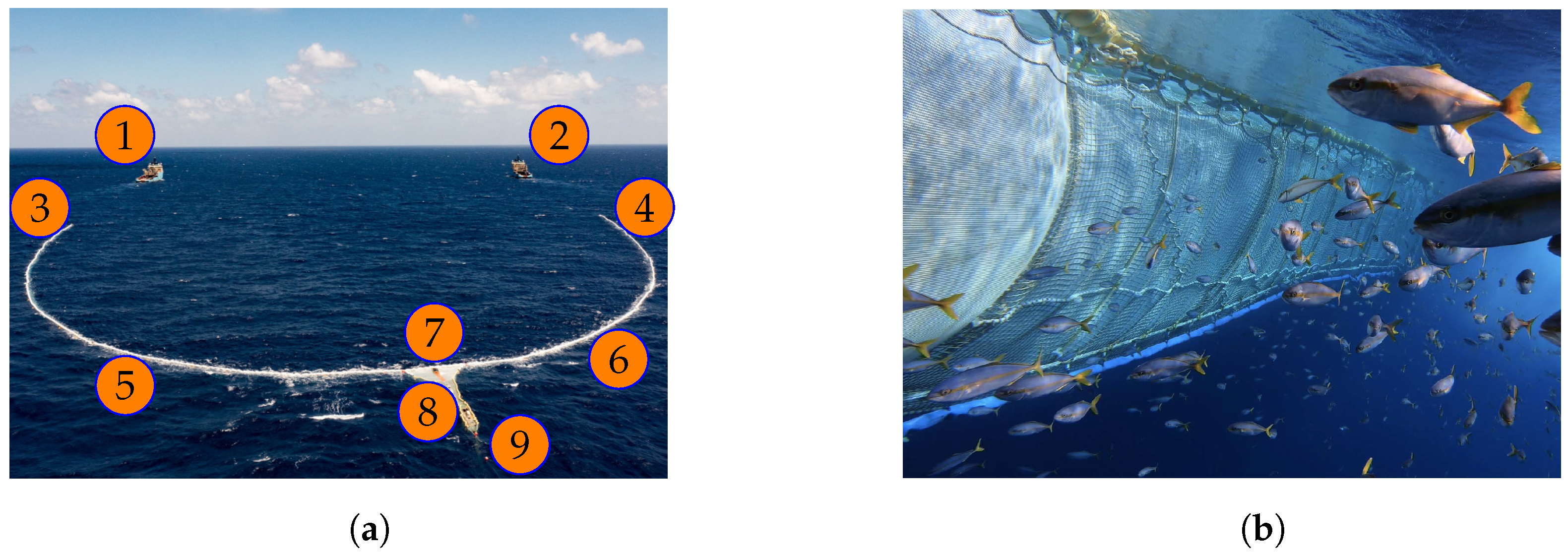
Figure 1. Above-water and underwater footage of System 002. Jmse 11 01943 i001 Port-side vessel. Jmse 11 01943 i002 Starboard-side vessel. Jmse 11 01943 i003 
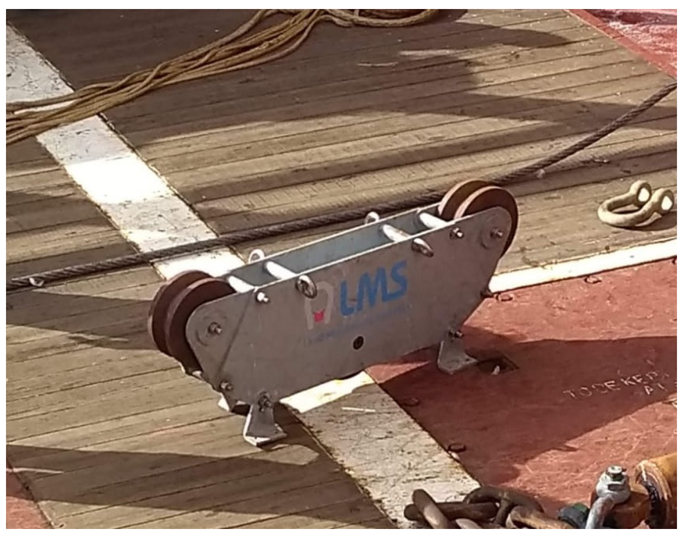
Port-side tow bar and towing bridle, connected to a towing line. Jmse 11 01943 i004 Starboard-side tow bar and towing bridle, connected to a towing line. Jmse 11 01943 i005 Port-side wingspan. Jmse 11 01943 i006 Starboard-side wingspan. Jmse 11 01943 i007 Retention opening. Jmse 11 01943 i008 Retention zone. Jmse 11 01943 i009 Extraction pick-up line. (a) Aerial view of System 002 towed by two vessels. (b) Underwater view of the retention zone made of nets.
Jmse 11 01943 g001
Figure 2. Running Line Monitor (RLM) to measure towline tension.
Jmse 11 01943 g002
Figure 3. Example comparison between u stw from DVL and u stw calculated with SOG-sea current.
Jmse 11 01943 g003
Figure 4. Local and global coordinate systems in OrcaFlex.
Jmse 11 01943 g004
Figure 5. Basic definition of a knot-less net.
Jmse 11 01943 g005
Figure 6. A twine in the wake of a leading twine. Illustration with dimensionless vorticity field from 2D direct numerical simulation.
Jmse 11 01943 g006
Figure 7. Method flowchart.
Jmse 11 01943 g007
Figure 8. Sketch of the system with basic definitions.
Jmse 11 01943 g008
Figure 9. Wing section model in OF.
Jmse 11 01943 g009
Figure 10. The 3D sketch of a plane net. Vertical twines in green color. Horizontal twines in red color. These colors are corresponding to the components of Equations (27) and (28).
Jmse 11 01943 g010
Figure 11. (a) Top view of Jenny’s wing modeled as collections of successive plane nets. (b) The 2D cross-sectional sketch of a plane net modeled as circular cylinders.
Jmse 11 01943 g011
Figure 12. Illustration of a complex boundary layer separation at R e t * = 1000 as seen in the research of Bouard and Coutanceau [47], Koumoutsakos and Leonard [48], Mohaghegh and Udaykumar [49] captured by Basilisk [33]. Vorticity field (top) and the quadtree structure (bottom).
Jmse 11 01943 g012
Figure 13. Illustration of the drag coefficient and the numerical parameters related to its computation. (a) Instantaneous drag coefficient at R e t * = 1000 for various smallest grid sizes. (b) Instantaneous drag coefficient at R e t * = 1600 for various smallest grid sizes. (c) Instantaneous number of cells for δ * 1 = 128 as a function of c at R e t * = 1000 . (d) Instantaneous number of cells for δ * 1 = 128 as a function of c at R e t * = 1600 . (e) Instantaneous drag coefficient for δ * 1 = 128 as a function of c * at R e t * = 1000 . (f) Instantaneous drag coefficient for δ * 1 = 128 as a function of c * at R e t * = 1600 .
Jmse 11 01943 g013
Figure 14. Close-up illustration of the shielding effect mechanism for θ = 8 ° at R e t * = 1000 . Blue and red, respectively, indicate negative and positive values of the vorticity fields.
Jmse 11 01943 g014
Figure 15. Illustration of the flow structure using the velocity field u x as a function of θ at R e t * = 1000 and t * = 90 . Blue and red, respectively, indicate low and high values of u x * .
Jmse 11 01943 g015
Figure 16. Influence of the number of twines N t * on the instantaneous total drag coefficient for various low angles of attack θ at R e t * = 800 .
Jmse 11 01943 g016
Figure 17. Dependence of the drag coefficient on the angle of attack. The median of the fluctuations is shown with the standard deviation.
Jmse 11 01943 g017
Figure 18. Dependence of the lift coefficient on the angle of attack. Median of the fluctuations is shown with standard deviation.
Jmse 11 01943 g018
Figure 19. Dependence of the combined towline tension on the u stw . Superscripts 16, 480, and 630 indicate the span in meters. The colored areas are the 15% increase in the mean load. GPGP data selected from August 2021 to August 2022. The error bar estimation is explained in Section 2.1.
Jmse 11 01943 g019
Figure 20. Distribution of the angles of attack.
Jmse 11 01943 g020
Figure 21. Schematic representation of the boundaries for the application of the results.
Jmse 11 01943 g021
Figure 22. Interdependence of the twine diameter, the mesh size, the solidity, and the drag coefficient of a net. Adapted from the work of Cheng et al. [13]. (a) Dependence of the solidity S n * on the twine diameter and the mesh size. (b) Dependence of the drag coefficient on the solidity for nylon nets at θ = 90 ° . (I) Tang et al. [59], (II) Gansel et al. [60], (III) Tsukrov et al. [61].
Jmse 11 01943 g022
Table 1. Span values for S L = 800 m.
Span TypeSpan (m)System RatioSystem Status
Narrow≈160.02Towing behind one vessel
Nominal≈4800.6Optimal performance in operation
Wide≈6300.8Maximize plastic catch
Table 2. Wave factors for several u stw and several sea states. () Annual non-exceeding probability in the GPGP considered location.
Sea State u stw (m/s)
a.n.e.p. (†) H s (m) T p (s)0.10.250.50.751.0
p251.710.83.831.741.191.091.11
p502.311.94.722.021.301.151.13
p753.011.96.772.621.541.281.19
p904.113.19.563.371.811.411.26
Table 3. Optimization cases.
Optimization CaseSpan TypeAngles
1Narrow 0 ° θ 2 °
2Nominal 30 ° θ 90 °
3Wide 45 ° θ 90 °
Table 4. Mesh cross flow drag coefficients ( C D , mem * ) for the 2nd and 3rd validation cycles.
θ ( ° )2nd Cycle3rd Cycle
901.59991.5967
451.59991.5589
301.59991.3822
201.55891.2649
100.56390.8492
50.20050.6076
30.09330.5253
20.05080.4849
10.01800.4732
00.00.4614
Table 5. Recommended axial drag coefficients ( C D , OF , a * ) for OrcaFlex System 002 model.
Span Type1st Cycle2nd Cycle3rd Cycle3rd Cycle—Averaged
Narrow0.2080.0100.0820.046
Nominal0.2080.3320.2850.285
Wide0.2080.3010.3240.324
Disclaimer/Publisher’s Note: The statements, opinions and data contained in all publications are solely those of the individual author(s) and contributor(s) and not of MDPI and/or the editor(s). MDPI and/or the editor(s) disclaim responsibility for any injury to people or property resulting from any ideas, methods, instructions or products referred to in the content.

