Probability Distribution Analysis of Hydrodynamic Wave Pressure on Large-Scale Thin-Walled Structure for Sea-Crossing Bridge

Abstract

Evaluation of hydrodynamic wave pressure on large-scale structure is an important task in the wave load design of thin-walled components used in sea-crossing bridge. This study focuses on the probability distribution of hydrodynamic wave pressure on a large-scale thin-walled structure using on-site measurement data. An in-situ observation project is conducted to collect the wave elevation and the wave pressure on a rectangle cofferdam during a tropical cyclone event. With the measured data, the wave conditions and the fluctuating wave pressure are extracted, and the corresponding statistical characteristics such as the cumulative density function (CDF) are derived. In addition, a time domain boundary element model (TDBEM) is introduced to provide the statistical comparison. Several wave conditions derived by the statistical wave indicators during the cyclone event are fed to the numerical model for pressure investigation. Based on the statistical indicators and the modeling results, the comparison of wave pressure spatial distribution between TDBEM and the on-site measurement is presented. The pressure probability distribution is presented to further reveal the differences on the statistical characteristics. The resultant bias mainly occurs in the low-exceeding-probability range on the up-wave side and the high-exceeding-probability range on the down-wave side.

1. Introduction

Wave load is one of the major environmental loads acting on the sea-crossing bridge [1,2,3], which may impact the dynamic behavior of the bridge and lead to some problems such as obvious structural response [4,5,6] and fatigue [7,8]. Moreover, in the construction stage, the extreme hydrodynamic pressure caused by high waves may severely threaten the safety of the bridge and other temporary structures [9,10,11]. With the concerns above, the wave load thus needs to be considered reasonably in both of design and construction.

Due to the relatively large radial dimension of the substructure, such as pylon and pier, wave diffraction may influence the wave field and result in the more complex wave load which is hard to be determined. The most intuitive way to obtain the wave load (usually evaluated as wave pressure) on the structure is to perform an on-site measurement (field measurement), which directly measures the wave pressure through various sensors or transducers. Many studies are conducted to improve the on-site measurement [12,13]. However, the pressure measurement with high labor and financial costs may be not so friendly for utilization, while another relatively concise way is to evaluate the wave pressure by numerical prediction.

Numerical simulation for ocean wave has been rapidly developed in recent years. The major simulation models extensively applied include finite element method (FEM) [14], finite volume method (FVM) [15], volume of fluid method (VOF) [16], and boundary element method (BEM) [17,18]. Among those modeling methods, boundary element method (BEM) shows the advantages that simplifying the dimension of problem (e.g., simplifying 3D problem to 2D) and reducing the computational complexity due to the discretization on the boundary surfaces instead of the whole fluid volume. However, BEM is usually applied in float body such as vessels and boats, and barely applied in bridge engineering. In this study, the time domain boundary element method (TDBEM) is developed and introduced for modeling ocean wave and evaluating pressure for a sea-crossing bridge. In numerical simulation for ocean wave, the representative wave method is commonly used [19,20,21], which transforms the actual random incident waves into a regular wave with certain wave conditions (wave height, period, etc.) according to the statistical characteristics. With the representative waves, the numerical simulation can reflect the actual wave pressure in a certain degree and provide the reference for design.

In general, due to the high cost of the on-site measurement, the measured wave data is hard to be obtained and seldom compared with TDBEM which is also less applied on structures, and it is meaningful to present the differences between the two methods in spatial and statistical distributions, which is barely studied and reported. In this study, based on a temporary cofferdam used in the construction of a sea-crossing bridge, the comparison of the wave pressures measured and predicted by TDBEM is carried out in both aspects of spatial distribution and statistical characteristics. Firstly, an on-site measurement was performed to record the time history of the incident wave elevation and the wave pressure through the wave elevation gauge and the pressure transducers, respectively. The incident wave height and the corresponding period are extracted from the wave elevation time history, and for the prediction by TDBEM with the representative wave method, several wave height statistical indicators such as average wave heights of the greatest $1/k$ waves $H_{1/k}$, including the significant height, are obtained through the cumulative density functions (CDFs) derived by the kernel density estimation (KDE) of the measured wave heights. Meanwhile, amplitude of the wave pressure on each transducer is also extracted, and similar with the wave height, through the cumulative density functions (CDFs) of the wave pressure amplitude, the statistical indicators for pressure amplitude, i.e., the average pressure amplitudes of the greatest $1/k$ amplitudes $P_{1/k}$, are obtained for comparing with the prediction. In addition, some other measured parameters which is useful to prediction and comparison such as still water level (SWL) and the main wave direction are also obtained by the measurement. Then, the theory of TDBEM is introduced and the prediction configurations are determined. According to the measured wave height, the representative wave method is applied into TDBEM to predict the wave pressure amplitude for comparing with the measured pressure indicators in spatial distribution. Afterwards, for further clarifying the differences between the measurement and TDBEM prediction in statistical characteristics, the pressure amplitude CDFs of the prediction are derived for comparing with the measurement. The differences in probability distribution are presented and discussed, then some conclusions are summarized at the end.

2. On-Site Measurement

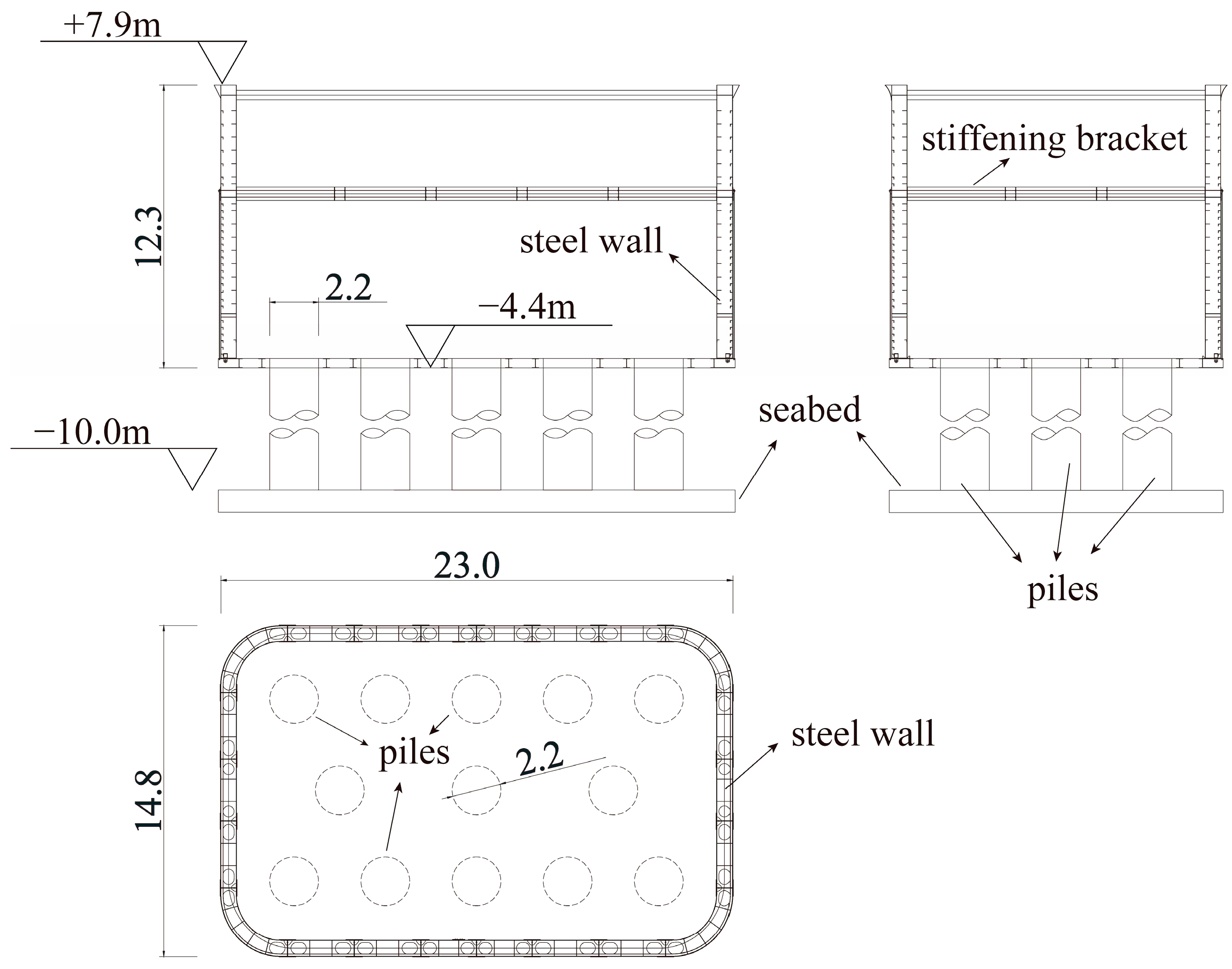
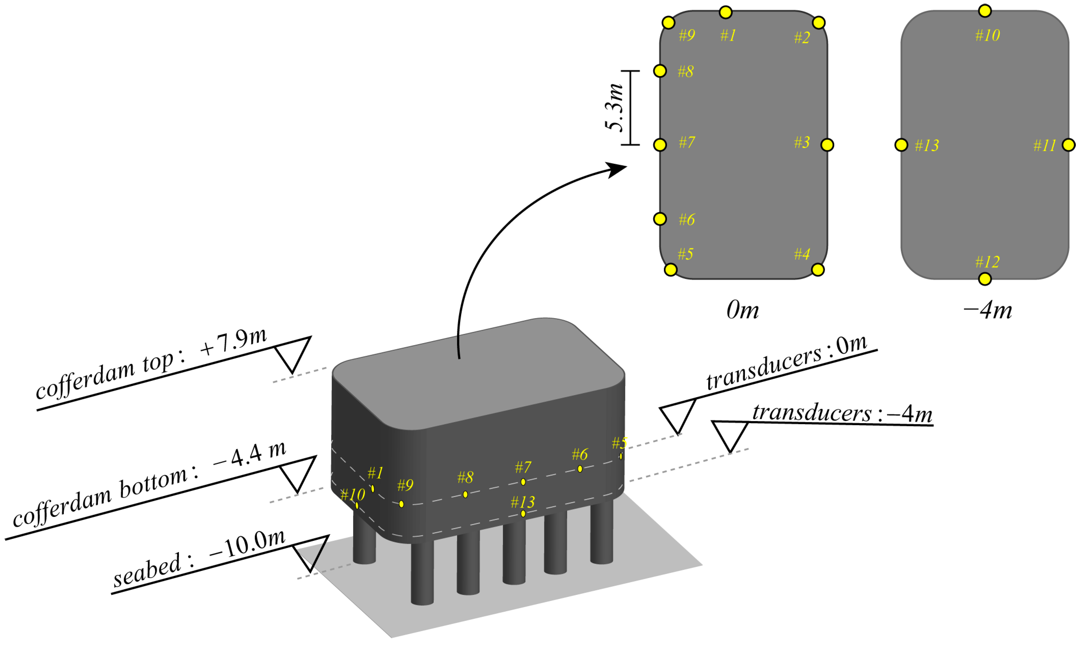
2.1. Case Discreption and Measurement Layout

Pingtan Strait Bridge is a 16.2 km long rail-road sea-crossing bridge in the China East Sea, connecting Fuzhou city and Pingtan Island, as shown in Figure 1. Due to the opened northeast offshore, the waves propagating from the northeast caused by cyclone may threaten the bridge under construction. For analyzing the impact of the destructive waves on construction of the bridge, a temporary cofferdam is taken for the on-site measurement, of which cross-sections are sketched in Figure 2. The thin-walled steel cofferdam locates at 25.72° N, 119.61° E, of which dimensions are 23.0 × 14.8 × 12.3 m. Below the cofferdam, 13 reinforced concrete piles with diameter of 2.2 m are used for supporting, and all of them are fixed on the seabed whose altitude is −10 m. The top and the bottom altitudes of the cofferdam are +7.9 m and −4.4 m, respectively.

The on-site measurement includes the measurements of wave elevation and wave pressure. The wave surface elevation was measured by a SBY 2-1 ultrasonic wave gauge whose measuring accuracy is ±0.2 m for wave height and ±0.25 s for wave period. The sampling frequency is set to 2 Hz, which is adequate for the most waves. As the measurement layout shown in Figure 1, the wave gauge is fixed on a cantilever connecting to the platform which supplies electric power for the gauge, and the 80 m distance between the platform and the cofferdam is set to reduce the interference of construction on the incident wave as possible. The seabed altitude of the platform is −9.3 m, approximately equal to the cofferdam of −10 m, which can thus ignore the wave shoaling effect, and the wave spectrums at the two locations can be considered the same.

For the hydrodynamic pressure measurement, thirteen CSW560 type pressure transducers are deployed around the cofferdam for the random wave pressures. The measurement range of the transducers is 0–200 kPa and the margin of error is within 0.5%, which is sufficient for the pressure measurement. Setup of the transducers is drawn in Figure 3. Among those transducers, nine of them, i.e., #1–#9, are deployed at altitudes of 0 m for capturing the wave pressure around the still water level (SWL), and the rest four transducers of #10–#13 are deployed at altitude of −4 m.

At 8:00 a.m., 29 September 2015, when the Typhoon Dujuan begun to decay, the on-site measurement was performed, in which the maximum wind speed reached 35 m/s. After 17 min of measurement, about 100 waves were captured, and the wave surface elevation and the pressure were recorded successfully.

With the measured wave elevation and the pressure, the analysis based on stochastic process is prepared to be performed for the statistical characteristics. The analysis can be divided into two parts, i.e., analysis for the measured wave elevation and the measured wave pressure. Through the measured wave elevation, still water level (SWL), wave heights and periods, cumulative distribution function (CDF) of wave height, and the average wave height of the greatest $1/k$ waves $H_{1/k}$, which is the statistical indicator for wave height used for the prediction later, can be obtained. While the main wave direction, the amplitude of wave pressure, CDF for pressure amplitude, and the average pressure amplitude of the greatest $1/k$ amplitudes $P_{1/k}$—which is the statistical indicator for wave pressure used for comparing with the prediction—can be derived with the measured wave pressure. Each method for the statistical characteristics will be briefly introduced later.

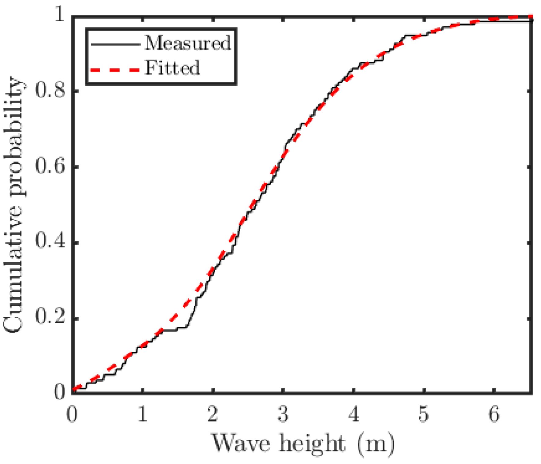
2.2. Wave Height and Period

Firstly, from the wave surface elevation time history, the wave heights can be extracted with the zero up-crossing method which is commonly used in many studies [22,23,24], and the period corresponding to each wave height is recorded. Then the probability density function (PDF) can be approximated by kernel density estimation (KDE), and the cumulative distribution function (CDF) can be further obtained by integration of the PDF, which indicates the probability of wave height $H$ lower than the specified value. Similar to the significant wave height, defining the average wave height of the greatest $1/k$ waves $H_{1/k}$ (Harish and Baba, 1986) as the statistical indicator for the wave height, which can be simply derived from the CDF as shown in Figure 4. A greater $k$ usually yields the less frequently encountered $H_{1/k}$, and when $k=1/3$, the $H_{1/3}$ denotes the significant wave height $H_s$. With respect to the wave period, each $H_{1/k}$ corresponds to the $T_{1/k}$ which equals the average period of those greatest $1/k$ waves. In addition, the average wave height $H_m$ and period $T_m$ are also obtained.

2.3. Still Water Level (SWL)

SWL can be measured by the ultrasonic wave gauge and was found to be +2.37 m during the measurement. The altitudes of the pressure transducers hence need to be altered, i.e., the altitudes of the transducers at the original 0 m and −4 m are shifted to −2.37 m and −6.37 m, respectively. In addition, the seabed altitude is also altered to −12.37 m from the original −10 m.

2.4. Wave Pressure and Direction

Similar to the wave height, the amplitude of wave pressure is extracted from the measured data, and the CDF of amplitude is obtained then. The maximum pressure $P_{\max }$ and the $P_{1/k}$, i.e., average pressure amplitude of the greatest $1/k$ amplitudes, are defined as the statistical indicators for the wave pressure, which is derived from the measured pressure and the CDF, respectively. Note that the analysis and comparison between the measurement and the prediction by TDBEM require the hydrodynamic wave pressure, thus the original measured wave pressure containing the hydrostatical component needs to be subtracted by the still water pressure according to the measured sinking depth of each transducer. In addition to the pressure, the wave direction also plays a dominant role in the prediction and comparison, which was measured by the time sequence that the transducers reach the peak pressure and it was found to be about 47° of the east–northeast.

3. Boundary Element Modeling in Time Domain

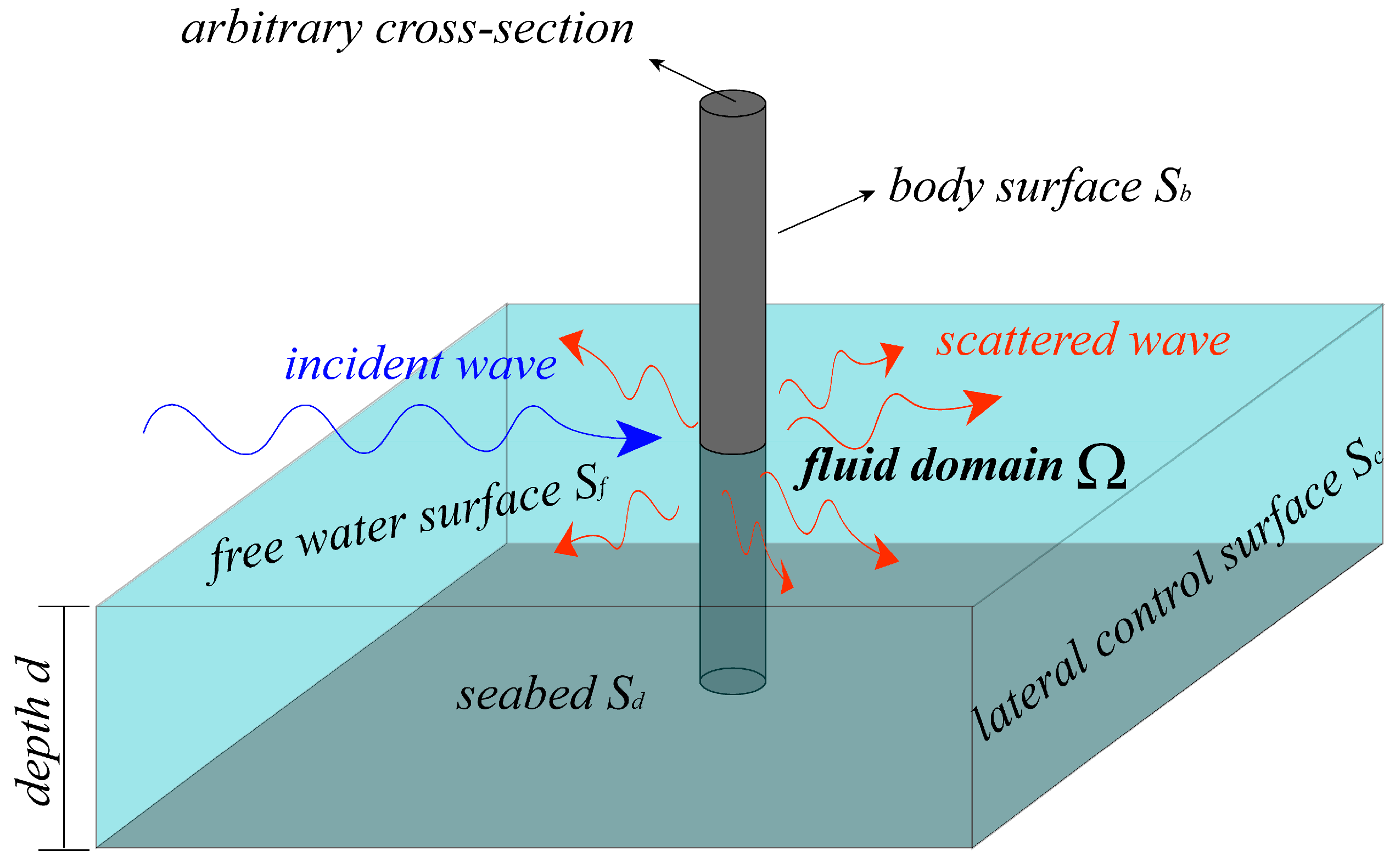
3.1. Fundamentals

When the lateral size of structure is closed to the incident wavelength, the scattered waves induced by diffraction are non-negligible and considerable, which will be superposed to the incident waves and eventually yield a new stable wave field. The fundamental problem of diffraction is shown in Figure 5, in which the fluid domain $\Omega$ with the water depth $d$ is incompressible and inviscid. With the free surface $S_f$ at the top, flat seabed $S_d$ at the bottom, and the lateral control surface $S_c$, the fluid domain $\Omega$ can be considered as a closed control volume. A rigid structure with an arbitrary cross-section (e.g., the cofferdam introduced above) is mounted on the seabed, of which body surface is denoted as $S_b$.

For the incompressible and inviscid fluid, flow potential theory is applied to expediently solve the problem. The time-variant velocity potential of wave $\Phi (x,t)$ meets the Laplace equation:

$${\nabla }^2\Phi (x,t)=0$$

(1)

in which $x$ is the location vector in right-hand Cartesian coordinate system, $x=(x,y,z)$. Since the wave field can be considered as a superposition of the incident and the scattered component, the potential and the water surface can be divided as

$$\Phi ={\Phi }_i+{\Phi }_s$$

(2)

$$\eta ={\eta }_i+{\eta }_s$$

(3)

in which the subscript $i$ refers to the incident components, i.e., ${\Phi }_i$ and ${\eta }_i$, which can be explicitly solved by Airy wave theory, while the subscript $s$ denotes the scattered components, i.e., ${\Phi }_s$ and ${\eta }_s$, which is the problem to be solved.

Before solving the scattered potential and the water surface function, the boundary conditions need to be defined clearly. The boundary conditions for the seabed, the free water surface, and the body surface can be listed as

$$\frac{\partial {\Phi }_s}{\partial z}=0\mathrm{on}{S}_d$$

(4)

$$\frac{\partial {\Phi }_s}{\partial z}-\frac{\partial {\eta }_s}{\partial t}=0\mathrm{on}{S}_f$$

(5)

$$\frac{\partial {\Phi }_s}{\partial t}+g{\eta }_s=0\mathrm{on}{S}_f$$

(6)

$$\frac{\partial {\Phi }_s}{\partial n}=-\frac{\partial {\Phi }_i}{\partial n}\mathrm{on}{S}_b$$

(7)

where $n$ denotes the normal vector on the body surface. For the lateral control surface $S_c$, an approach developed by Bai [25] is applied, which simulates the boundary of $S_c$ by constructing a physics-based beach zone:

$$\gamma (r)=\left\{\begin{array}{l}\alpha \omega {\left(\frac{r-r_0}{l}\right)}^2{r}_0\le r\le r_1=r_0+\beta l\\ 0r<r_0\end{array}\right.$$

(8)

where $\gamma$ is the damping coefficient; $r$ denotes the distance to the origin; $r_0$ is the starting point of the damping zone; $\omega$ and $l$ are wave frequency and wavelength, respectively; $\alpha$ and $\beta$ are the custom parameters defined by user, which is able to alter the damping behavior and is usually defined as 1 [25]. With such an approach, a damping zone whose performance acts like a sort of beach is constructed to hinder the wave motion and eliminate the reflection from the lateral control surface, and thus the lateral control surface can be excluded from the boundary surfaces to simplify the computation. With inserting the damping coefficient Equation (8) into Equations (5) and (6), the free surface boundary conditions in the damping zone can be expressed as

$$\frac{\partial {\eta }_s}{\partial t}=\frac{\partial {\Phi }_s}{\partial t}-\gamma (r){\eta }_s$$

(9)

$$\frac{\partial {\Phi }_s}{\partial t}=-g{\eta }_s-\gamma (r){\Phi }_s$$

(10)

With the Laplace governing equation and the boundary conditions above, the fundamental problem is fully illustrated. Before discretizing and solving the problem, a simplification can be performed by introducing the second Green’s theorem which can transform the three-dimensional volume integral to the two-dimensional surface integral on the boundary surfaces. With the second Green’s theorem, the computation can be further reduced, and the time domain integration formulation of the fundamental problem is obtained:

$$2\pi {\Phi }_s(\upsilon ,t)={\displaystyle {\iint }_S\left[{\Phi }_s(x,t)\frac{\partial G(x,\upsilon )}{\partial n}-G(x,\upsilon )\frac{\partial {\Phi }_s(x,t)}{\partial n}\right]}\mathrm{d}s$$

(11)

In which $x(x,y,z)$ and $\upsilon (\upsilon ,\nu ,\zeta )$ are the field and the source point, respectively; $G(x,\upsilon )$ is the Green function indicating the propagation property of velocity potential; the integral domain $s$ includes the body surface $S_b$, free water surface $S_f$, and the seabed surface $S_d$. Due to the flat and impermeable seabed, it can be excluded from the integral domain by appropriately selecting the simple Green function considering the symmetry about the seabed [17].

After the simplifications above, the body surface $S_b$ and the free water surface $S_f$ can be discretized to finite quadrilateral panels. According to some existing studies [17,26], the discretization of Equation (11) can be expressed as below when the source point is located on the body surface:

$$\begin{array}{l}2\pi {\Phi }_s({\upsilon }_i)-{\displaystyle \sum _{j=1}^{N_b}{\displaystyle {\int }_{\Delta S_j}{\Phi }_s(x_j)\frac{\partial G({\upsilon }_i,x_j)}{\partial n}ds}}+{\displaystyle \sum _{j=1}^{N_f}{\displaystyle {\int }_{\Delta S_j}G({\upsilon }_i,x_j)\frac{\partial {\Phi }_s(x_i)}{\partial n}ds}}=\\ {\displaystyle \sum _{j=1}^{N_f}{\displaystyle {\int }_{\Delta S_j}{\Phi }_s(x_j)\frac{\partial G({\upsilon }_i,x_j)}{\partial n}ds}}-{\displaystyle \sum _{j=1}^{N_b}{\displaystyle {\int }_{\Delta S_j}G({\upsilon }_i,x_j)\frac{\partial {\Phi }_s(x_j)}{\partial n}ds}}i=1\mathrm{to}{N}_b\end{array}$$

(12)

while the source point is located on the free water surface, the discretization can be rewritten as

$$\begin{array}{l}-{\displaystyle \sum _{j=1}^{N_b}{\displaystyle {\int }_{\Delta S_j}{\Phi }_s(x_j)\frac{\partial G({\upsilon }_i,x_j)}{\partial n}ds}}+{\displaystyle \sum _{j=1}^{N_f}{\displaystyle {\int }_{\Delta S_j}G({\upsilon }_i,x_j)\frac{\partial {\Phi }_s(x_i)}{\partial n}ds}}=\\ {\displaystyle \sum _{j=1}^{N_f}{\displaystyle {\int }_{\Delta S_j}{\Phi }_s(x_j)\frac{\partial G({\upsilon }_i,x_j)}{\partial n}ds}}-{\displaystyle \sum _{j=1}^{N_b}{\displaystyle {\int }_{\Delta S_j}G({\upsilon }_i,x_j)\frac{\partial {\Phi }_s(x_j)}{\partial n}ds}}-2\pi {\Phi }_s({\upsilon }_i)i=1\mathrm{to}{N}_f\end{array}$$

(13)

in which $N_b$ and $N_f$ are the numbers of the body surface and the free water surface respectively. In the equations above, the known terms are put on the right side, and the unknown terms which is to be solved are arranged on the left side.

The discretized equations above have clarified the potential solution at one single time step. With certain numerical integration method such as Gaussian integration, the unknown potentials on the body surface and the normal derivatives on the free surface can be obtained. Afterwards, the time-stepping procedure can be launched with certain numerical method such as the Adams-Bashforth method [27] or the Newmark method [28] to obtain the free surface elevation and the potential at the next time step. With the solved potential then, the hydrodynamic pressure on the structure can be derived by the first order Bernoulli equation:

$$p=-\rho \frac{\partial \Phi (x,t)}{\partial t}$$

(14)

in which $\rho$ denotes the fluid density.

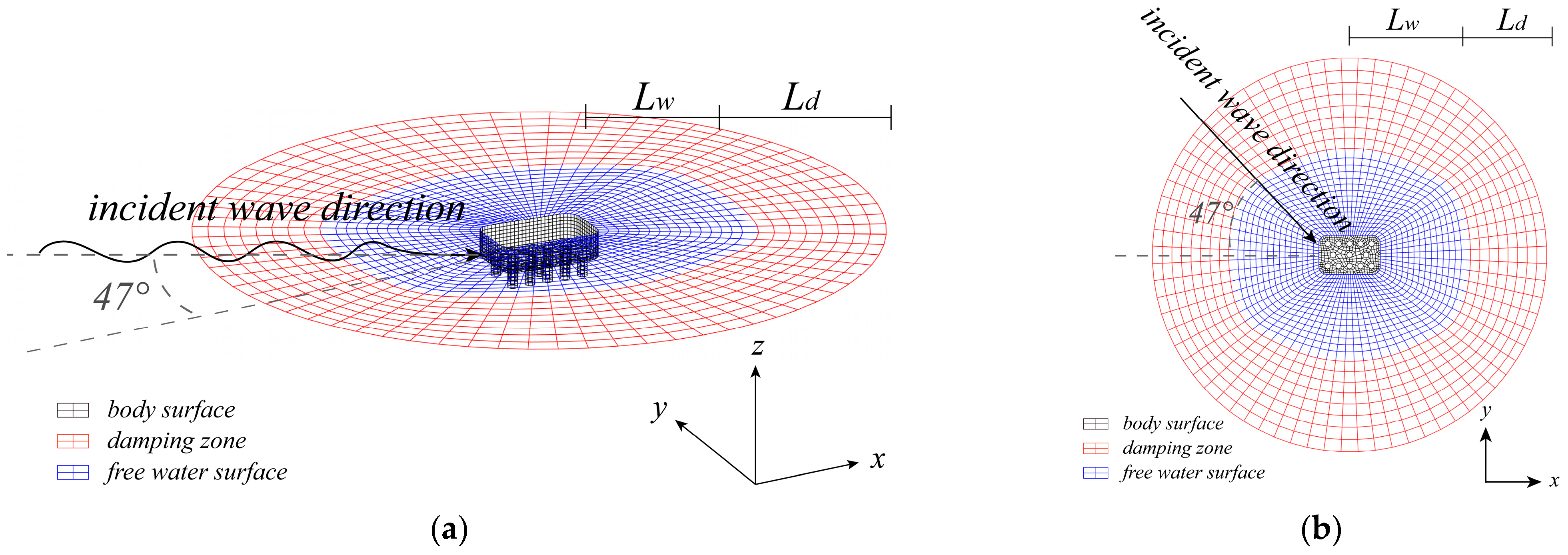
3.2. Mesh and Prediction Configurations

With the approach introduced above, the example cofferdam can be properly meshed for the numerical prediction. Note that, for the mesh quality of structures with various cross-sections, meshing under the polar coordinate system is benefit and reasonable, which can efficiently reduce the sharp corners in the mesh. Under the polar system, the mesh is performed along the three dimensions, i.e., the tangential dimension, the radial dimension, and the vertical dimension. According to the on-site measurement, the water depth is set to 10 m. Due to the relatively complex geometry of the cofferdam, the tangential dimensions of the free surface and the body surface are both divided into 72 partitions to ensure the sufficient accuracy. The radial and the vertical dimensions are divided into 25 and 10 partitions respectively. Due to the non-circular geometry, the mesh in the tangential dimension gradually transitions from the pattern of the cofferdam cross-section to a circle, along the radial direction. Lengths of the free water surface $L_w$ and the damping zone $L_d$ along the major axis of the cofferdam are both set to the incident wavelength $l$ to ensure the sufficient wave diffraction. Mesh of the cofferdam is shown in Figure 6.

With the cofferdam mesh, representative wave method is utilized for prediction, i.e., the actual random wave is represented by a regular wave with certain height and period determined by the statistical indicators for the measured wave height. According to the measurement, the wave direction is set to 47° of the east–northeast. With properly selecting the measured wave height statistical indicators $H_{1/k}$ and the period $T_{1/k}$ as the representative wave height and period, the TDBEM can hence predict the hydrodynamic wave pressure for comparing with the measurement.

4. Probability Analysis and Comparison

For comparing the wave pressures of TDBEM with the on-site measurement, according to some existed studies [29,30,31], the prediction conditions consisting of the measured wave height indicator $H_{1/k}$ and the corresponding period $T_{1/k}$ are specified as $H_{1/100}$ and $T_{1/100}$, $H_{1/100}$ and $T_m$, $H_{1/10}$ and $T_{1/10}$, $H_{1/3}$ and $T_{1/3}$. The wave height $H_{1/k}$ and corresponding period $T_{1/k}$ has been introduced in Section 2.2. Among those $H_{1/k}$, $H_{1/100}$ is to evaluate the wave pressure caused by the greatest part of waves. $H_{1/3}$, i.e., the significant wave height, is selected to evaluate the significant pressure like the common analysis. For more comparison data to discuss the differences between the prediction and the measurement, the wave height $H_{1/10}$ between $H_{1/100}$ and $H_{1/3}$ is also selected for supplementing the prediction.

With the selected $H_{1/k}$ and corresponding periods, wave pressure amplitudes at the transducers’ locations can be predicted by TDBEM. Then, with the known wave pressure statistical indicators $P_{1/k}$, the comparison of wave pressure spatial distribution around the cofferdam can be carried out to present the differences between the measurement and the TDBEM prediction. In addition to the pressure spatial distribution, cumulative distribution functions (CDFs) of the predicted pressure amplitudes can be derived through the wave height CDF, i.e., each wave height input into TDBEM yields the corresponding wave pressure amplitudes around the cofferdam, and with a simple variable substitution, the CDF of wave height (wave height against probability) can be transformed into the CDFs of pressure amplitude (amplitude against probability). With the pressure amplitude CDFs predicted and measured, through the comparison of probability distributions, the hydrodynamic wave pressure differences of the two methods in statistical characteristics will be further discussed.

5. Results and Discussions

5.1. Measurement Results

As introduced in Section 2, the wave surface elevation was measured by the wave gauge, of which result is shown in Figure 7. According to the result, about 17 min of wave elevation was recorded, and for sake of conciseness, the mean elevation is zeroized. The crests and troughs are marked with red circles, of which standard deviations (Std.) are given by the dash lines.

From the measured wave elevation, the wave height is extracted, and the probability distribution (CDF) can be obtained then. The CDF derived by KDE and fitted with Rayleigh’s distribution is shown in Figure 8. According to the CDF, it is found that the wave height range of 1.5–4 m corresponds to the relatively wider probability range, which indicates that the majority of wave heights distribute in the 1.5–4 m range. With the CDF and the representative wave method, the prediction conditions are obtained and listed in

Table 1. Prediction conditions derived from the measured waves.

Prediction Condition	Wave Height (m)	Period (s)
$H_{1/100}$, $T_{1/100}$	6.06	10.25
$H_{1/100}$, $T_m$	6.06	7.44
$H_{1/10}$, $T_{1/10}$	5.04	9.76
$H_{1/3}$, $T_{1/3}$	4.04	9.41
$H_m$, $T_m$	2.62	7.44

, which provides the input wave heights and periods for the TDBEM prediction.

For presenting the wave pressure measurement results concisely, instead of the large amount of the original measured data, the CDFs for wave pressure amplitudes of the transducers are shown and fitted with Rayleigh’s distribution in Figure 9 and Figure 10. Among the CDFs, #1–9 are the results for the transducers located at the altitude of −2.37 m and #11–13 show the results for the altitude of −6.37 m.

5.2. Wave Pressure Distribution Comparison Using Representative Waves

With the representative wave method introduced in 3.2 and the prediction conditions, the wave pressure amplitudes predicted by TDBEM are obtained for comparing with the pressure indicators from the measurement. The wave pressure statistical indicators of each transducer and the corresponding prediction results are detailly listed in

Table 2. Measurements ($P_{\max }$ and $P_{1/100}$ ) and predictions ($H_{1/100}$, $T_{1/100}$ and $H_{1/100}$, $T_m$ ).

Transducer	Measurement (kPa)		Prediction (kPa)
	${\mathit{P}}_{\mathbf{max}}$	${\mathit{P}}_{1/100}$	${\mathit{H}}_{1/100}$$,{\mathit{T}}_{1/100}$	${\mathit{H}}_{1/100}$$,{\mathit{T}}_{\mathit{m}}$
#1	36.24	34.06	31.64	33.07
#2	36.89	35.74	35.18	37.19
#3	33.63	33.72	33.46	37.97
#4	22.91	22.07	26.90	27.62
#5	18.07	18.59	24.05	19.65
#6	20.93	20.21	23.95	19.23
#7	15.95	15.70	23.85	19.16
#8	30.60	30.24	24.38	20.59
#9	26.39	25.08	26.39	24.96
#10	14.04	13.82	26.83	24.38
#11	21.46	20.87	26.36	25.23
#12	14.60	16.95	20.06	14.01
#13	17.76	17.84	19.66	13.01

,

Table 3. Measurement ($P_{1/10}$ ) and prediction ($H_{1/10}$, $T_{1/10}$ ).

Transducer	Measurement (kPa)	Prediction (kPa)
#1	27.60	26.48
#2	28.97	29.57
#3	28.24	28.22
#4	19.77	22.36
#5	15.45	19.63
#6	16.49	19.53
#7	13.41	19.45
#8	24.35	19.95
#9	21.37	21.80
#10	12.17	22.17
#11	16.60	21.85
#12	13.50	16.14
#13	15.40	15.77

and

Table 4. Measurement ($P_{1/3}$ ) and prediction ($H_{1/3}$, $T_{1/3}$ ).

Transducer	Measurement (kPa)	Prediction (kPa)
#1	22.26	21.37
#2	23.15	23.96
#3	23.24	22.98
#4	16.50	17.93
#5	12.95	15.41
#6	13.42	15.32
#7	11.15	15.25
#8	20.05	15.70
#9	18.42	17.36
#10	10.00	17.64
#11	13.20	17.45
#12	11.03	12.46
#13	12.76	12.13

, and the comparison is shown in Figure 11 and Figure 12, which presents the pressure amplitude spatial distributions at the altitudes of −2.37 m and −6.37 m, respectively. For the better visualization of the spatial distributions, the figures are drawn as a contour-like plot with several isopleths of pressure. Figure 11a,b and Figure 12a,b indicate that the prediction conditions of $H_{1/100}$, $T_{1/100}$ and $H_{1/100}$, $T_m$ derive the almost same pressure amplitude results, which means that the both wave periods can reflect the pressure induced by the greatest part of the wave heights. At the altitude of −2.37 m, the favorable agreements are shown in each subplot, particularly for the pressure amplitude predicted by $H_{1/3}$ and the measured $P_{1/3}$. The bias mainly occurs near the down-wave side, while the gap between the prediction and the measurement is negligible and can hence be ignored. At the altitude of −6.37 m, good agreements are shown except the result of #10 that the prediction is greater than the measurement. In Figure 12, the largest bias at #10 reaches about 50% of the predicted pressure, while the gap is gradually narrowed with decreasing of the input wave height $H_{1/k}$. For example, in Figure 12d, with the significant wave height $H_{1/3}$ input, the predicted pressure amplitude of #10 is close to the measured. From the overall view, the pressure amplitude distributions predicted by TDBEM indicate an acceptable agreement with the on-site measurement, and the error mainly exists at the certain location of #10 which has a relatively large water depth.

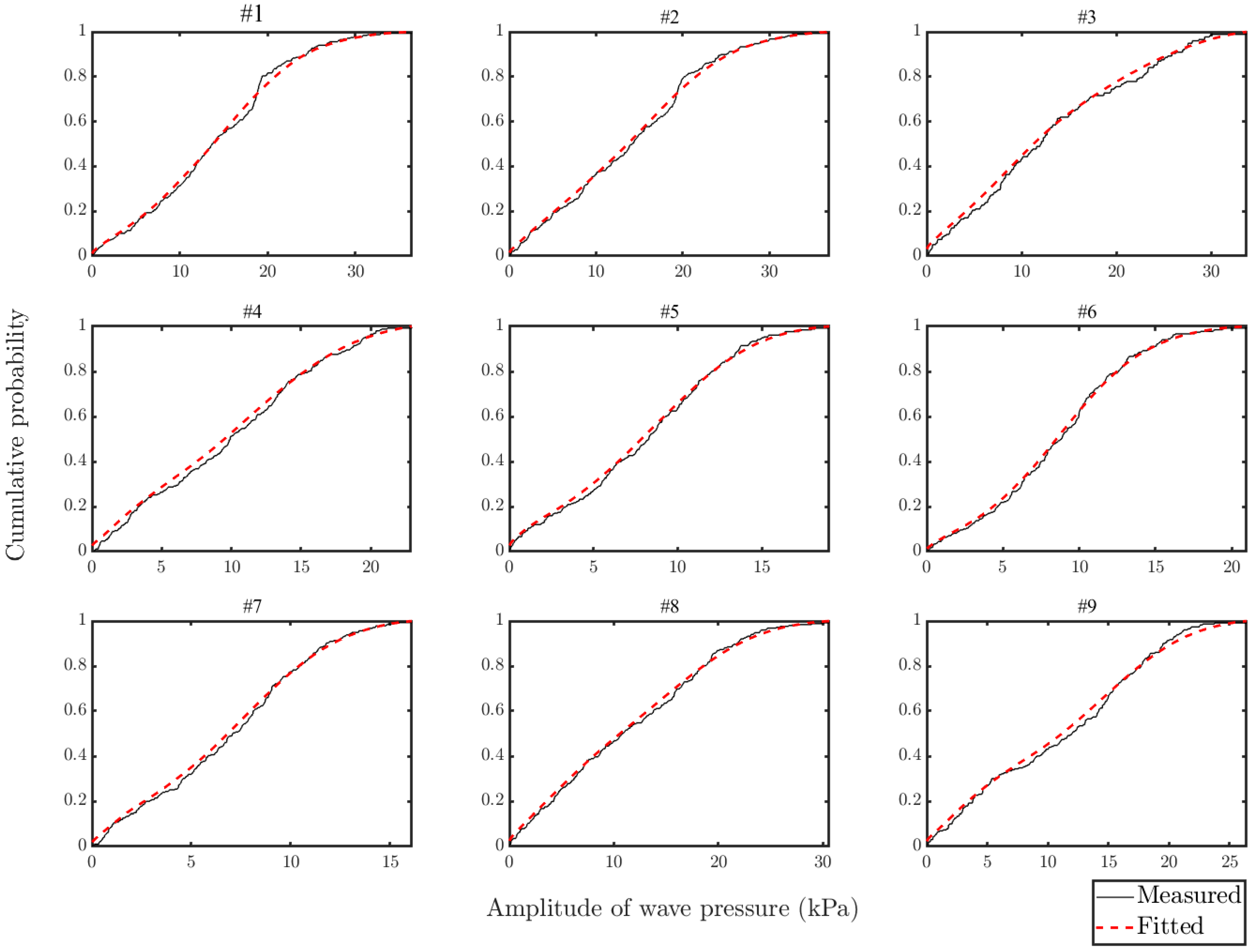
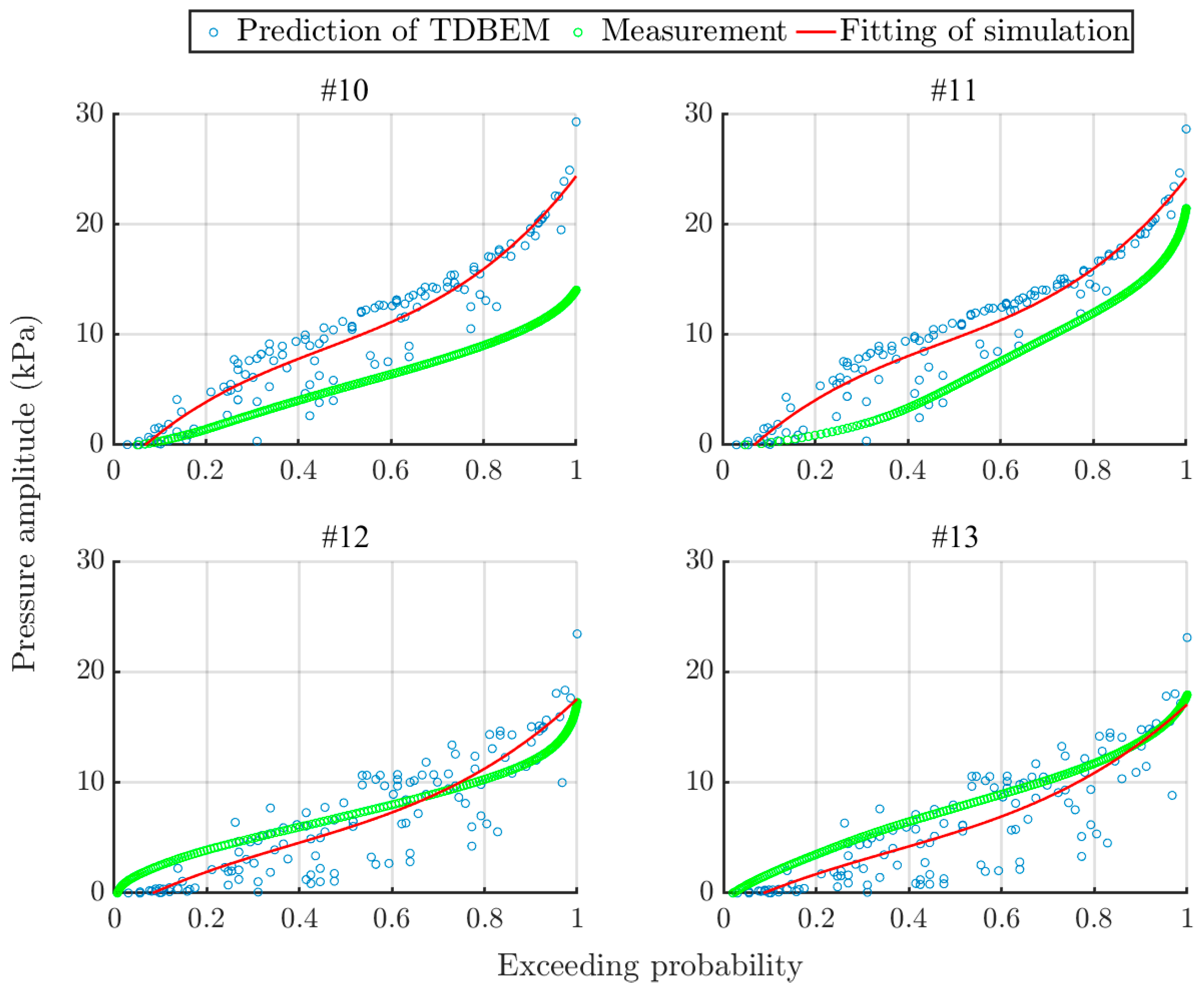
5.3. Wave Pressure Comparison Using Probability Distribution

The wave pressure spatial distribution comparison using the representative wave method and the statistical indicators exactly shows the differences between the TDBEM prediction and the on-site measurement. Still, the comparison in probability distribution is necessary for presenting the differences in greater detail, which is able to show the difference in pressure amplitudes at each probability level. With the CDF of the measured wave height, the CDFs of the predicted pressure amplitude can be derived, and the comparison between the measured and the predicted CDFs can be carried out, as shown in Figure 13 and Figure 14.

For the discussion, the horizontal axis is assigned to the exceeding probability and the vertical is the pressure amplitude. Each subplot illustrates the comparison at each transducer location. The green scatter plot shows the probability distribution of the measured wave pressure amplitude, while the blue shows the predicted probability distribution which is fitted by the red line. In the comparison at the altitude of −2.37 m, as shown in Figure 13, the error mainly occurs in the low-exceeding-probability range of the transducers located in the up-wave side, i.e., the results of #2–#4 whose predictions are greater than the measurements. While in the down-wave side, the error mainly occurs in the high-exceeding-probability range, such as #7 and #8, among which the prediction of #7 is greater than the measurement while it is contrary for #8. At the altitude of −6.37 m, the predictions in the up-wave side are greater than the measurements as shown in results of #10 and #11, while the predictions in the down-wave side are relatively lower than the measurements over the low-exceeding-probability range, as shown in results of #11 and #12. In addition, with increasing the water sinking depth, the margin of error in the comparison is increased, particularly for the up-wave side, which accounts for the large bias occurred in the previous comparison of pressure spatial distribution.

6. Conclusions

This article aims to present the hydrodynamic wave pressure comparison between the on-site measurement and the numerical prediction modeled by time domain boundary element method (TDBEM). Based on the temporary cofferdam used in the construction of Pingtan Strait Bridge, the on-site measurement is introduced and was performed during the Typhoon Dujuan in 2015. The wave height and period, still water level (SWL), and the wave pressure and direction were successfully recorded during the 17 min of measurement. Several statistical indicators such as the average wave height of the greatest $1/k$ waves $H_{1/k}$ and the average wave pressure amplitude of the greatest $1/k$ pressure amplitudes $P_{1/k}$ are derived from the measured data for the prediction and the comparison. Afterwards, the statistical wave conditions are fed to the pressure prediction using a TDBEM model. The time-stepping integration is employed to drive the prediction using the first and fourth order Adams–Bashforth equations, through which the time-variant potential can be hence solved. With the measured and predicted pressure results, the comparisons of the pressure spatial distribution and the probability distribution are analyzed and discussed, from which several major conclusions are summarized as follows:

(1)

In the spatial distribution of the wave pressure amplitude, a favorable agreement is shown at the altitude of −2.37 m, of which the prediction is slightly greater than the measurement on the down-wave side. While at the altitude of −6.37 m, the water depth obviously impacts the results and leads to a relatively large bias at the location of the #10 transducer. However, with decreasing the representative wave height, the gap between the prediction and the measurement is gradually narrowed.

(2)

In the probability distribution of the wave pressure amplitude, the pressure amplitude against exceeding probability at each transducer is presented. At the altitude of −2.37 m, decent agreements are shown in most of the results. The error mainly occurs in the low-exceeding-probability range in the up-wave side and the high-exceeding-probability range in the down-wave side. With increasing the water depth, at the altitude of −6.37 m, the margin of error is greater than the −2.37 m and compared with the down-wave side, the biases are more significant in the up-wave side, which accounts for the relatively large bias which occurred in the pressure spatial distribution.

Since the major scope of this study is to present a comparison of statistical characteristics, in the future, more comprehensive research should be carried out to further discuss the hydrodynamic wave pressure differences between TDBEM and the measurement, particularly for the relatively large bias on the up-wave side at a larger water depth. Another limitation should be noted that the second-order nonlinear wave effect is absent in the presented study to reduce the complexity of the problem and is worth investigating in the future.

References

1. Guo, A.; Fang, Q.; Bai, X.; Li, H. Hydrodynamic experiment of the wave force acting on the superstructures of coastal bridges. J. Bridge Eng. 2015, 20, 04015012. [Google Scholar] [CrossRef]
2. Ti, Z.; Zhang, M.; Li, Y.; Wei, K. Numerical study on the stochastic response of a long-span sea-crossing bridge subjected to extreme nonlinear wave loads. Eng. Struct. 2019, 196, 109287. [Google Scholar] [CrossRef]
3. Chen, X.; Chen, Z.; Xu, G.; Zhuo, X.; Deng, Q. Review of wave forces on bridge decks with experimental and numerical methods. Adv. Bridge Eng. 2021, 2, 1. [Google Scholar] [CrossRef]
4. Chen, L.; Zang, J.; Hillis, A.J.; Morgan, G.C.; Plummer, A.R. Numerical investigation of wave–structure interaction using OpenFOAM. Ocean. Eng. 2014, 88, 91–109. [Google Scholar] [CrossRef] [Green Version]
5. Xiang, T.; Istrati, D. Assessment of Extreme Wave Impact on Coastal Decks with Different Geometries via the Arbitrary Lagrangian-Eulerian Method. J. Mar. Sci. Eng. 2021, 9, 1342. [Google Scholar] [CrossRef]
6. Finnegan, W.; Goggins, J. Numerical simulation of linear water waves and wave–structure interaction. Ocean. Eng. 2012, 43, 23–31. [Google Scholar] [CrossRef] [Green Version]
7. Yeter, B.; Garbatov, Y.; Guedes Soares, C. Spectral Fatigue Assessment of an Offshore Wind Turbine Structure under Wave and Wind Loading. In Developments in Maritime Transportation and Exploitation of Sea Resources; Taylor & Francis Group: London, UK, 2014; pp. 425–433. [Google Scholar]
8. Zhu, J.; Zhang, W. Probabilistic fatigue damage assessment of coastal slender bridges under coupled dynamic loads. Eng. Struct. 2018, 166, 274–285. [Google Scholar] [CrossRef]
9. Hasanpour, A.; Istrati, D. Extreme Storm Wave Impact on Elevated Coastal Buildings. In Proceedings of the 3rd International Conference on Natural Hazards & Infrastructure (ICONHIC2022), Athens, Greece, 5–7 July 2022; pp. 5–7. [Google Scholar]
10. Hua, L. Hydrodynamic problems associated with construction of sea-crossing bridges. J. Hydrodyn. Ser. B 2006, 18, 13–18. [Google Scholar]
11. Ti, Z.; Wei, K.; Qin, S.; Mei, D.; Li, Y. Assessment of random wave pressure on the construction cofferdam for sea-crossing bridges under tropical cyclone. Ocean. Eng. 2018, 160, 335–345. [Google Scholar] [CrossRef]
12. Bishop, C.T.; Donelan, M.A. Measuring waves with pressure transducers. Coast. Eng. 1987, 11, 309–328. [Google Scholar] [CrossRef]
13. Joodaki, G.; Nahavandchi, H.; Cheng, K. Ocean wave measurement using GPS buoys. J. Geod. Sci. 2013, 3, 163–172. [Google Scholar] [CrossRef]
14. Hasanpour, A.; Istrati, D.; Buckle, I. Coupled SPH–FEM Modeling of Tsunami-Borne Large Debris Flow and Impact on Coastal Structures. J. Mar. Sci. Eng. 2021, 9, 1068. [Google Scholar] [CrossRef]
15. Liang, Z.; Jeng, D.-S.; Liu, J. Combined wave–current induced seabed liquefaction around buried pipelines: Design of a trench layer. Ocean. Eng. 2020, 212, 107764. [Google Scholar] [CrossRef]
16. Zhao, X.-Z.; Hu, C.-H.; Sun, Z.-C. Numerical simulation of extreme wave generation using VOF method. J. Hydrodyn. Ser. B 2010, 22, 466–477. [Google Scholar] [CrossRef]
17. Isaacson, M.; Cheung Kwok, F. Time-Domain Second-Order Wave Diffraction in Three Dimensions. J. Waterw. Port Coast. Ocean. Eng. 1992, 118, 496–516. [Google Scholar] [CrossRef]
18. Ti, Z.; Li, Y.; Qin, S. Numerical approach of interaction between wave and flexible bridge pier with arbitrary cross section based on boundary element method. J. Bridge Eng. 2020, 25, 04020095. [Google Scholar] [CrossRef]
19. Chesher, T.; Miles, G. The Concept of a Single Representative Wave for Use in Numerical Models of Long Term Sediment Transport Predictions, Hydraulic and Environmental Modelling; Routledge: London, UK, 2019; pp. 371–380. [Google Scholar]
20. Dibajnia, M.; Moriya, T.; Watanabe, A. A representative wave model for estimation of nearshore local transport rate. Coast. Eng. J. 2001, 43, 1–38. [Google Scholar] [CrossRef]
21. Rattanapitikon, W.; Karunchintadit, R.; Shibayama, T. Irregular wave height transformation using representative wave approach. Coast. Eng. J. 2003, 45, 489–510. [Google Scholar] [CrossRef]
22. Hwang, S.; Lim, C.; Lee, J.L. Extraction of nearshore spectrum by energy-conserved zero-up crossing method and comparison with the TMA spectrum. Ocean. Eng. 2021, 241, 109962. [Google Scholar] [CrossRef]
23. Lin, J.-G.; Lin, Y.-F.; Hsu, S.-Y.; Chiu, Y.-F. A Combined Empirical Decomposition and Zero-Up-Crossing Method on Ocean Wave Analysis. In Proceedings of the Twentieth International Offshore and Polar Engineering Conference, Beijing, China, 20–25 June 2010. [Google Scholar]
24. Manohar, M.; Mobarek, I.; El Sharaky, N. Characteristic Wave Period. In Proceedings of the 15th International Conference on Coastal Engineering, Honolulu, HA, USA, 11–17 July 1976; pp. 273–288. [Google Scholar]
25. Bai, W.; Teng, B. Simulation of second-order wave interaction with fixed and floating structures in time domain. Ocean. Eng. 2013, 74, 168–177. [Google Scholar] [CrossRef]
26. Isaacson, M.; Cheung, K.-F. Time-domain solution for second-order wave diffraction. J. Waterw. Port Coast. Ocean. Eng. 1990, 116, 191–210. [Google Scholar] [CrossRef]
27. Choi, C.-Y.; Balaras, E. A dual reciprocity boundary element formulation using the fractional step method for the incompressible Navier–Stokes equations. Eng. Anal. Bound. Elem. 2009, 33, 741–749. [Google Scholar] [CrossRef]
28. Oyarzún, P.; Loureiro, F.; Carrer, J.; Mansur, W. A time-stepping scheme based on numerical Green’s functions for the domain boundary element method: The ExGA-DBEM Newmark approach. Eng. Anal. Bound. Elem. 2011, 35, 533–542. [Google Scholar] [CrossRef]
29. Harish, C.; Baba, M. On spectral and statistical characteristics of shallow water waves. Ocean. Eng. 1986, 13, 239–248. [Google Scholar] [CrossRef]
30. Putz, R. Statistical distributions for ocean waves. Eos Trans. Am. Geophys. Union 1952, 33, 685–692. [Google Scholar] [CrossRef]
31. Vandever, J.P.; Siegel, E.M.; Brubaker, J.M.; Friedrichs, C.T. Influence of spectral width on wave height parameter estimates in coastal environments. J. Waterw. Port Coast. Ocean. Eng. 2008, 134, 187–194. [Google Scholar] [CrossRef]
Figure 1. The on-site measurement location and layout.
Jmse 11 00081 g001
Figure 2. Cross-sections of the cofferdam.
Jmse 11 00081 g002
Figure 3. Setup of the transducers.
Jmse 11 00081 g003
Figure 4. The relationship between H 1 / k and the CDF.
Jmse 11 00081 g004
Figure 5. Foundamental problem of wave diffraction.
Jmse 11 00081 g005
Figure 6. Mesh of the cofferdam. (a) Stereoscopic view; (b) Vertical view.
Jmse 11 00081 g006
Figure 7. Time history of the measured wave height.
Jmse 11 00081 g007
Figure 8. CDF of the measured wave height.
Jmse 11 00081 g008
Figure 9. CDFs of the measured wave pressure amplitude at −2.37 m.
Jmse 11 00081 g009
Figure 10. CDFs of the measured wave pressure amplitude at −6.37 m.
Jmse 11 00081 g010
Figure 11. Pressure spatial distributions at −2.37 m. (a) H 1 / 100 , T 1 / 100 (b) H 1 / 100 , T m (c) H 1 / 10 , T 1 / 10 (d) H 1 / 3 , T 1 / 3 .
Jmse 11 00081 g011
Figure 12. Pressure spatial distributions at −6.37 m. (a) H 1 / 100 , T 1 / 100 (b) H 1 / 100 , T m (c) H 1 / 10 , T 1 / 10 (d) H 1 / 3 , T 1 / 3 .
Jmse 11 00081 g012
Figure 13. Probability distributions of the pressure amplitude at −2.37 m.
Jmse 11 00081 g013
Figure 14. Probability distributions of the pressure amplitude at −6.37 m.
Jmse 11 00081 g014