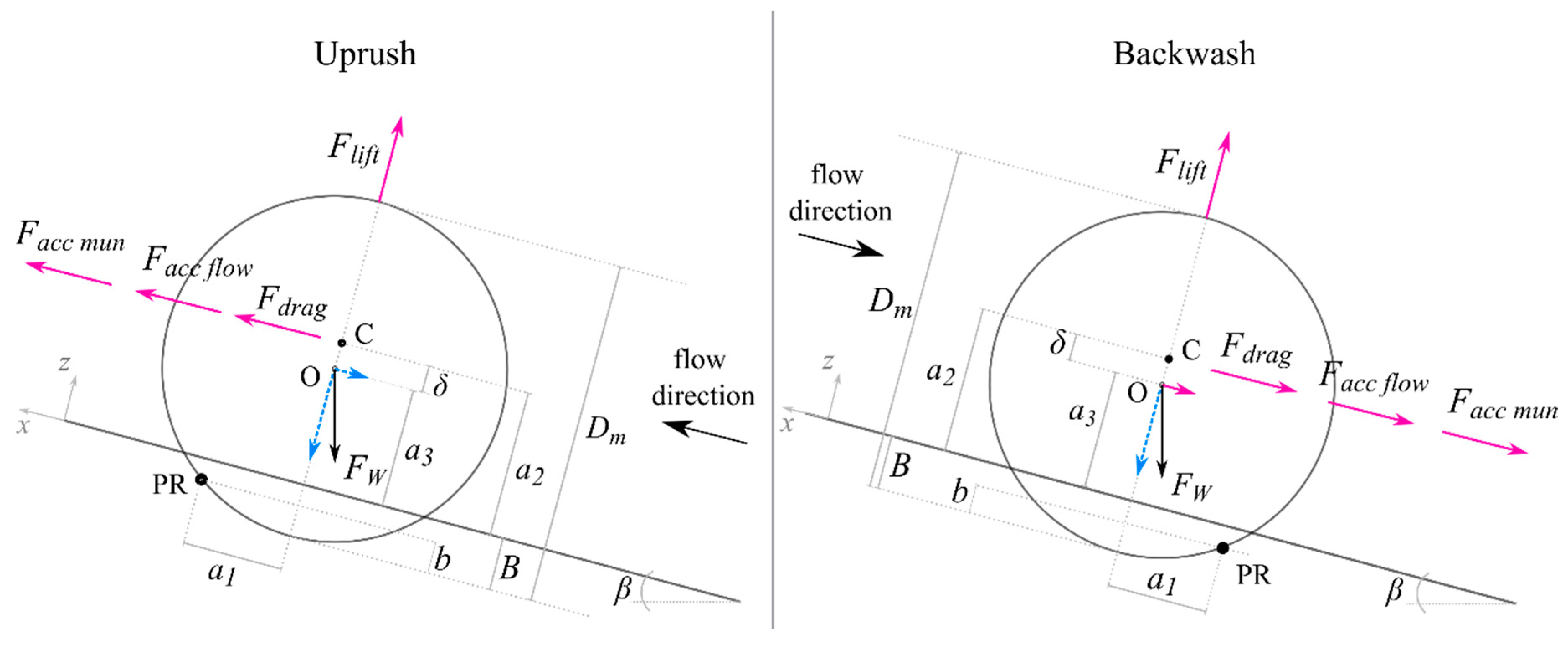
Article

Momentum Balance Analysis of Spherical Objects and Long-Term Field Observations of Unexploded Ordnance (UXO) in the Swash Zone

1
Marine and Coastal Risk Management, JBA Consulting, Edinburgh EH14 4AP, UK
2
Olsen Associates, Inc., Jacksonville, FL 32204, USA
3
Center for Applied Coastal Research, University of Delaware, Newark, DE 19716, USA
*
Author to whom correspondence should be addressed.
J. Mar. Sci. Eng. 2023, 11(1), 79; https://doi.org/10.3390/jmse11010079
Submission received: 23 November 2022 / Revised: 18 December 2022 / Accepted: 21 December 2022 / Published: 3 January 2023
(This article belongs to the Section Coastal Engineering)

Abstract

:
Military activity has resulted in unexploded ordnance (UXO) existing in the nearshore. Understanding and predicting UXO behavior is important for object identification, and management. Here, two studies (laboratory and fieldwork) have been conducted to observe UXO surrogates in the swash zone and relate burial and migration to the underlying forcing conditions. A small-scale laboratory dam-break study was conducted to quantify migration of varying density spherical objects at different locations on a sloping, mobile, sandy bed. A moment balance was applied to derive two data-driven relationships to: (1) predict moments from the cross-shore flow velocity with predictions confined within a factor of two; (2) predict upslope or downslope migration from the moment. Fitting coefficients for the upslope and downslope relationships vary as a function of density, initial position, and burial. A field study was also conducted to investigate long-term behavior of eight varieties of UXO surrogates. Of the 129 observations, 56% were mobilized of which 76% were directed offshore. Burial/exposure was mostly related to far-field beach accretion/erosion (67%). However, scouring processes were also observed. Data showed that migration is likely a short-term process and most munitions will ultimately scour into a mobile bed.

1. Introduction

The swash zone is the nearshore environment where wave bores run up the beach. It extends from the limit of run-down to the limit of wave run-up [1,2]. The swash zone is a dynamic environment where wave motion continuously rushes up and down the beach face (also called foreshore). Sediment transport along and across the beach face may be significant depending on forcing conditions. In addition, isolated objects may be found resting on the beach face as a result of offshore-onshore migration due to wave forcing or as a result of beach morphodynamics that lead to object exhumation.
Larger sediment grains, cobbles, (0.064–0.256 m in size) or boulders (>0.256 m) may be present on the beach due to high-energy events (storms or tsunamis). Some experimental and modeling efforts have been conducted to determine the applicability of theoretical formulations for cobble motion in the swash and surf zones [3,4,5]. Many other studies have been carried out on boulder motion with the aim to develop mobility models and an inverse estimate of the magnitude of the high-energy event [6,7,8,9,10].
Intense military activity carried out in the past resulted in the presence of a large quantity of unexploded ordnance (UXO) on coastal seafloors worldwide including over 400 formerly used defense sites in the US [11]. Identifying and possibly retrieving UXO are crucial for safety reasons as beaches are used for recreational activities. Understanding UXO behavior, mobility, and burial, in relation to the forcing conditions is fundamental for UXO localization and determining if UXO pose a threat to human receptors [12]. Probabilistic predictive models of mobility exist [13] but require additional data to improve the range of applicable conditions. Field observations of munition mobility are scarce [14,15] and were generally obtained seaward of the swash zone. Swash zone field data on munition mobility do not exist to the authors’ knowledge. Thus, field data are needed to improve predictive models and especially long-term observations to mimic real-world scenarios.
Burial and migration of objects were investigated through a variety of laboratory experiments under various hydrodynamic conditions. Burial of short cylinders subjected to combined waves and currents was found to strongly depend on the Shields parameter and the Keulegan-Carpenter number [16]. This dependance is also the case for cylinders under oscillatory flows [17]. However, the equilibrium burial depth was observed to be larger for oscillatory flows when compared to wave-current forcing [17]. The dependency between burial and dimensionless numbers was also confirmed by a study that synthetized a compilation of available published data [18]. In the compilation paper, the critical object mobility number of underwater cylinders under steady flows was expressed as a function of the ratio between object diameter and bed roughness. Modifications to the critical mobility number were made for accelerating flows where competing mechanisms of scour burial and critical shear stress exist. More recently, observations of objects and surrogate munitions were collected under active surf and swash zone conditions [19,20,21]. Discrete correlation between burial and migration with dimensionless numbers was observed in the swash zone [20]. Although less dense munitions and steeper beach slopes were deemed responsible for greatest migration distances, UXO response under intense swash zone hydrodynamics is highly variabile [20].
In this paper two data sets are used to investigate UXO behavior on a sloping mobile bed. (1) A laboratory study was conducted in a small-scale flume to determine UXO behavior under dam-break forcing. UXO were deployed at different cross-shore positions on the beach slope and with three different initial burial depths. Repeatability tests were conducted to assess variability, with a total of 275 runs. The laboratory results were used to calculate forces exerted to the objects and perform a moment balance analysis to investigate initiation of motion. (2) A field experiment was carried out for over two months. The aim of the study was to observe long term UXO behavior in a natural environment comprehensive of beach morphodynamics, tides, and varying wave forcing conditions. Measurements of hydrodynamics and morphology were collected, while munitions of different shapes, sizes, and densities, originally deployed at the beach face at the beginning of the experiment, were free to be mobilized by the forcing. In addition, observations of five different types of munitions subjected to a single swash event were acquired for additional object force balance analysis.
The present study provides two comprehensive datasets of UXO in the swash zone to support future UXO predictions and probabilistic model calibration and validation. The analysis carried out assists in parametrizing UXO migration on the beach face in relation to the local hydrodynamics. Ultimately, the goal of this work is to contribute to coastal risk management and localization of UXO.

2. Methodology

2.1. Momentum Balance of an Intermittently Submerged Object Resting on a Sloping Beach Face

Object migration on the beach face due to varying forcing conditions is a complex phenomenon. The complexity is attributed to a series of factors: (1) the sandy bed represents a permeable and mobile surface, interacting with the object that may induce scour; (2) the physical properties of the object, such as shape, density, dimensions, and roughness of external surface, alter transport characteristics; (3) object orientation relative to the flow direction alters mobility; and (4) variations in the flow characteristics such as directional variability and water depth add more components to the problem. An additional difficulty is that the parameters that govern object motion vary in time and space and are difficult to estimate with fixed instrumentation and Eulerian measurements.
Swash events are constituted by two phases: uprush and backwash. During uprush, the flow is onshore-directed with a generally decelerating flow field [22]. A mobilized object may, perhaps through uprush impingement, travel upslope. During backwash, the flow is offshore-directed and accelerates downslope under gravity. The flow may decelerate in the latter stages as friction dominates the thinning flow. Objects may be more difficult to mobilize with the flow starting from rest. However, once mobilized, fluid forcing and gravity acting in unison may enable farther migration distance than during uprush [20,23]. Depending on the environment, type of object, and forcing conditions, different modes of transport occur. Sliding and saltation may be analyzed through the object motion equation that applies a balance of forces to the body.
The rolling mode of transport, more common for cylindrical and spherical munitions, is investigated and schematized here. Only cross-shore rolling motion, the main component of motion, is addressed in this study. The analysis requires consideration of the moments around the point of rotation [23,24], different between uprush and backwash phases (point PR in Figure 1). The two-dimensional (2D) coordinate system consists of an x-axis aligned with the slope of the beach face and a z-axis orthogonal to it. The forces acting on the object are drag, Fdrag, lift, Flift, flow acceleration, Facc flow, munition acceleration, Facc mun, reduced gravity, FW, and friction Ffriction. The forces are expressed as [3]:
F d r a g = 1 2 C d ρ w A d | u | u ,
F l i f t = 1 2 C l ρ w A l | u | u ,
F a c c   f l o w = ( 1 + C m ) ρ w V m du dt u | u | ,
F a c c   m u n = ( ρ m + ρ w C m ) V m d u m dt u m | u m | ,
F W = ( ρ m ρ w ) V m g ,
F f r i c t i o n = C f V m ( ρ m ρ w ) gcos ( β ) ,
with Ad the area of the munition facing the flow, Al the area of the object facing up, u the cross-shore flow velocity, um the munition cross-shore velocity, ρ w the water density (~1000 kg/m3), ρ m, Dm and Vm the munition density, diameter and volume, respectively, g the gravitational acceleration (9.81 m/s2), and β the angle between the beach slope and the horizontal.
Four coefficients appear in the force expressions: coefficients of drag, Cd, lift, Cl, added mass, Cm, and friction, Cf. The drag and lift coefficients vary depending on the flow condition, the geometry of the object, and other external factors. For simplicity, the drag coefficient is often provided as a function of the instantaneous Reynolds number of the object defined as [3]:
R e m = ( u u m ) v D m .
The added mass coefficient accounts for the acceleration of the water around the object. Cm increases when the swash impacts the object and is related to the ratio between the water depth and the object diameter [25]. The friction coefficient parametrizes the interactions between the munition and the bed during munition motion. It is tedious, if not impossible, to find the most appropriate value for each coefficient, especially considering the temporal variability. Most often constant coefficient values are used (Table 1). Here, the value 1 is used for all coefficients.
The sign of flow-related forces depends on the flow direction while the munition acceleration depends on the munition motion, if motion occurs. Friction is always opposite to flow direction or opposite to munition motion. Reduced gravity is always vertical and can be decomposed to downslope and slope-orthogonal components.
An assumption is made that the object can move only in the cross-shore direction, either upslope or downslope, by rolling around the point of rotation (point PR in Figure 1). The mobility of the object is determined by comparing the summation of the stabilizing moments that act against the motion, M+, and the summation of the destabilizing moments that induce the object to roll in the flow direction, M. The resulting moment M is defined as:
M = | M | | M + | .
Therefore, when M + exceeds M (negative M) the object remains in place, otherwise (positive M) the object will move. The following equations express stabilizing and destabilizing moments for the two swash phases (highlighted in blue or magenta depending on whether they are associated with M + or M in Figure 1):
  • Uprush
M + = F W   c o s ( β ) a 1 + F W   s i n ( β ) a 3 .
M = F l i f t a 1 + F d r a g a 2 + F a c c   f l o w a 2 + F a c c   m u n a 2 .
  • Backwash
M + = F W   c o s ( β ) a 1 .
M = F W s i n ( β )   a 3 + F l i f t a 1 + F d r a g a 2 + F a c c   f l o w a 2 + F a c c   m u n a 2 ,
where a1, a2 and a3 are the force moment arms relative to point PR. The moment arms are simplified through the following expressions (after [24]):
a 1 = b ( D m b ) ,
a 2 = D m 2 + δ b ,
a 3 = D 2 b   ,
with b the distance between PR and the base of the object and Δ the distance between points C and O (Figure 1), These two distances are expressed as:
b = λ B ,
δ = B 2 .
where B is the burial depth (Figure 1). The factor λ is a function of the dimensionless burial depth, B/Dm, and ranges from 0.44 and 0.49 for B/Dm between 0 and 1 [24].

2.2. Dimensionless Parameters Related to Object Migration and Burial

Burial and migration of objects (e.g., cobbles, cylinders, surrogate munitions) subjected to various forcing conditions (e.g., oscillatory flows, waves with and without a superimposed current, accelerating flow, swash) were related to dimensionless numbers through empirical formulations [5,18,20,26,27,28]. The dimensionless numbers most often related to burial are the Keulegan-Carpenter number, KC, and the Shields parameter, θ. Migration, on the other hand, is usually related to the object mobility number, θm, [8]. Most recently for the swash zone, the Iribarren number, ξ, that accounts for beach slope and offshore forcing, was also included [20]. The empirical formulations derived for migration usually include one or more of these dimensionless numbers.
KC represents the ratio between drag and inertia forces while θ represents the ratio between destabilizing and stabilizing forces for sediment mobilization. They are expressed as:
K C = u T D m ,
θ = τ b ( ρ s ρ w ) g d 50 ,
where here T is the swash duration, ρs is the sediment density (2650 kg/m3), d50 the median sediment grain size, and τb the bed shear stress. The bed shear stress is estimated roughly via the drag law as
τ b = 1 2 ρ w f | u | u ,
with f being a friction coefficient set equal to 0.03 [29]. The object mobility number is defined as:
θ m = | u | u ( ρ m ρ w 1 ) g D m ,
which includes the object diameter and density. The object mobility number is mostly used to study initiation of motion and identify the threshold for motion/no motion. A modified object mobility number considering the initial burial depth, Bi, may be more appropriate if the munition is partially buried prior to mobilization:
θ m   m o d = | u | u ( ρ m ρ w 1 ) g D m D m B i D m .

3. Laboratory Study

3.1. Experimental Setup and Procedure

The laboratory study was conducted in the wave flume located at the Center for Applied Coastal Research (CACR) at the University of Delaware (Newark, NJ, USA) during June, July and August of 2018 to test object mobility and burial in the swash zone. The utilized part of the flume is 9.42 m long and 0.6 m wide (Figure 2). The sloping sandy bed, composed of a median grain diameter d50 = 0.31 mm, was established over the last 4.8 m with a slope tanβ = 1:7 (8 degrees). A dam-break scenario was used to create a single swash event with the gate retaining a reservoir of water (0.73 × 1.00 × 0.57 m3). The retained fluid was released by rapidly lifting the reservoir gate and it propagated down the flume as a broken bore. The bore impinged the sloping bed and initiated swash.
Water levels, flow velocity, object migration and final burial depth, were collected during the experiment. Only those sensors that provided measurements used for the analysis carried out in this paper are mentioned here. Considering the width of the flume, the experimental procedure consisted in measuring the hydrodynamics and the object response separately (mainly to prevent sensor damage due to object mobility and avoid view obstruction in object tracking from the overhead camera). Thus, a set of 10 runs was first conducted to assess the hydrodynamic conditions. Multiple runs were used to verify repeatability of the hydrodynamics within the flume. The runs where objects were deployed contained no corresponding swash zone hydrodynamic measurements. It is assumed that the objects were tested under the same forcing conditions based on the repeatability studies.
Water level was recorded at 10 cross-shore locations using resistance wave gauges (WG) mounted on the flume wall recording at 16 Hz and Banner ultrasonic distance meters (UDM) mounted on carts along the flume wall recording at 8 Hz (Figure 2). Valeport electromagnetic current meters (EM) recording at 8 Hz were used to determine velocity at the toe of the beach and at the locations where objects were deployed. The EMs were positioned roughly 0.02 m above the bed. A wide-angle field of view camera (Prosilica GT1920, 3.5 mm lens) recording at 30 frames per second (fps) was deployed from overhead to capture the object response through video-imagery. A Velodyne Puck lidar system with a motor speed of 600 RPM and data collecting at 10 Hz was mounted above the flume and used to monitor bed variability during reshaping procedures and morphologic change after each swash event.
Time synchronization for WGs, UDMs and EMs was performed using a dedicated time server consisting of Tac32 and Dimension4 software and a Garmin GPS module. The time server received Coordinate Universal Time (UTC) from accessible satellites and distributed this time to the computers logging sensor data. A coordinate system was implemented with the origin set to the toe of the sloping bed and an x-axis aligned with the slope of the beach face pointing onshore and an upward z-axis (Figure 2) matching the coordinate system shown in Figure 1.
The objects tested in this study were surrogates of the nearly spherical BLU-26, BLU-61, BLU-63 Cluster Bomb [30]. Multiple varieties of the Cluster Bomb exist with different diameters (~0.060–0.100 m) and densities (~2900–5000 kg/m3). The objects used here were spherical (no spin-arm flutes as the real munition) with Dm = 0.0769 m and fabricated in four variations: concrete ( C o ,   ρ m = 1800 kg/m3); aluminum ( A l ,   ρ m = 2700 kg/m3); lead-core with a galvanized steel shell ( G S ,   ρ m = 4200 kg/m3); and solid stainless steel ( S S ,   ρ m = 7700 kg/m3). The experimental procedure consisted of deploying each object type at various configurations of initial cross-shore position and burial depth (Table 2) totaling 54 scenarios (Table 3). The three variables of initial position, initial burial depth, and density would yield a total number of 60 = 5 × 3 × 4 (positions × burial × density) scenarios. However, the two densest objects (GS and SS) were not tested under the initial burial depths of 0.3 (B2) and 0.5 (B3) at initial position 13.4 m (P4) and under the initial burial depth of 0.5 (B3) at initial position 14 m (P5) due to lack of motion under preliminary tests. Each scenario is identified with a tag using the acronyms specified in Table 2. For example, the scenario where the stainless steel object was tested at position P4 and burial status B2 is identified by the tag SSP4B2. Five to ten repetitions per scenario were run depending on response variability. However, some runs were discarded after quality control routines. Hence, the number of repetitions per scenario varied between 3 and 9 totaling 275 runs.
A series of procedures was performed every testing day and prior to each run to reduce experimental boundary condition variations and to capture the probabilistic nature of object response under repeated morphological and hydrodynamic conditions:
(1)
A wave was launched in the flume before starting a new set of runs to ‘wet’ the sediment in the flume, so each subsequent run had the initial conditions of a wet beach face.
(2)
The UDM mounted above the reservoir (UDM-GATE) was checked to verify the initial water depth, accepting a maximum error of 2 mm from the 0.73 m target depth.
(3)
The beach was reset manually after each run using a heavy-slider weight with a metal track that was pulled across the beach surface. The Velodyne lidar was used to quantify the bed surface elevation by calculating a root-mean-square error (RMSE) of the smoothed bed compared to an ideal 1:7 profile. A RMSE < 3 mm relative to the baseline slope was maintained for each run.

3.1.1. Hydrodynamic Measurements and Processing

Water depth from WGs was determined through a calibration from voltage to measured water depth. Water depth from UDMs was calculated by subtracting detected distances from the surveyed sensor height. Ensemble averaging techniques were used to quantify variability in the experiment and determine representative hydrodynamics for the swash event (Figure 3a–p). Water level and velocity measurements obtained from the 10 hydrodynamic test repetitions were aligned to relative time using the UDM-GATE signal as a time datum when the free surface in the reservoir exceeded a 0.1 m/s change rate. Aligned data were then ensemble-averaged for approximately 9 s at each sensor position. Disregarding data after the appearance of the reflected wave in the time signal ~7 s after initiation, the UDM-GATE exhibited a standard deviation of less than ±0.01 m for about 85% and less than ±0.02 m for about 95% of the event (Figure 3a). The other five UDMs exhibited a standard deviation less than 0.01 m for 91% and less than 0.015 m for 97% of the event (Figure 3g–k). The WGs were stationed immediately downstream from the gate where the most turbulence occurred and together exhibited a standard deviation less than ±0.01 m for 83% and ±0.015 cm for 92% of the event (Figure 3b–f). The standard deviation for velocity was less than ±0.14 m/s for 90% of the event for the five EMs (Figure 3l–p). Runup was manually traced from rectified imagery captured from the overhead camera through the creation of time stacks. Time stack construction entails plotting a georeferenced transect of pixels on the y-axis over the entire swash duration. Plotting pixels in this manner allows for a depiction of the entire swash event (Figure 3q).
Timeseries of the hydrodynamics are essential to calculate forces and moments. Ideally, h and u are needed at the object location at each timestep during the swash event. Although objects were initially deployed at cross-shore locations ranging from P1 to P5, where velocity measurements were collected and thus available, objects could migrate either upslope or downslope during the swash event. Additionally, water level sensors were not deployed at locations P1-P5. Thus, h and u were spatially interpolated (in the cross-shore direction) for each run based on the object instantaneous position along the slope. The object migration path was always confined within the locations of UDM2 and UDM5, for all runs. Thus, the water level was easily interpolated having always a value of h landward and seaward of the instantaneous object location. On the other hand, unfortunately, velocity data were not available throughout the entire swash event and objects sometimes travelled outside the distance P1-P5 (EM locations). The beginning of the uprush is not captured by the EM due to the initial submergence [22]. A few criteria were set to carry out the interpolation. If the instantaneous object position fell within two positions of available velocity data, the instantaneous velocity was found as a spatial interpolation. If the object position was instead spatially outside the available measurements, if the distance between the object and the closest measurement was less than 0.15 m, the instantaneous velocity was set to that value otherwise was not assigned. The velocity was linearly extrapolated back in time to an h of 0.02 m to capture the beginning of the uprush. Ultimately thisis the cross-shore velocity used for moment calculations and going forward will be referred to as u for simplicity.

3.1.2. Object Tracking Technique

A motion-based technique was used to quantify object cross-shore position in the geo-referenced image sequence [31,32]. The objects were painted green to facilitate identification (contrasting color to that of the background). The object motion tracking technique entailed applying a mask to each frame, which excluded all pixels not within the flume. Next, each raw image was split into red-green-blue pixels, and after choosing the most intense green pixels, a morphological enhancement was performed to select the two largest clusters of pixels. In this case, the ‘green-most’ pixels were selected. The clusters were enhanced to be the only identifiable features in the image. Manual selection of spheres on rectified images was also performed in cases where the automatic tracking failed due to poor visibility.
This series of modifications was applied throughout time to track the sphere trajectory. A cost assignment was applied after every detection to maintain the spheres as separate objects. The spheres were not identifiable in every frame, especially when first impacted by swash and when they were transported during backwash to the highly turbulent region at the toe of the beach. A Kalman filter was applied to predict the new location based on past detections. The Computer Vision Toolbox in Matlab was used to apply these corrections and maintain a time series of sphere detections. The algorithm fails upon bore impact (~2 s) and at offshore locations less than ~0.5 m. Time series smoothing and input of manually identified surrogate locations were used to supplement the time series. Final surrogate locations were recorded after each run and used as the final position in the trajectory time series.
The object distance travelled obtained from the imagery is referred to as dx if referenced to the x-axis of the flume (Figure 2) and dxi if referenced to the initial object position.

3.2. Migration

The 54 scenarios were analyzed individually to determine an average object response and quantify the associated variability. Time series of cross-shore flow velocity and object distance travelled were averaged across the repetitions tested per each scenario. For each repetition, the standard deviations, σu and σx for cross-shore velocity and distance travelled, respectively were determined (for the whole time series) to assess variability. For example, if a scenario was repeated five times, five values of σu and σx would be obtained. Although mean and maximum σu did not exceed 0.1 m/s and 0.16 m/s, respectively (Figure 4a), runs belonging to the same scenario showed object response variability in some cases (Figure 4b). Object response variability is not unexpected given the turbulent nature of the flow field and potentially small differences in initial object conditions. The maximum σx almost reached 0.8 m, with a few other cases showing travel distances exceeding 0.3 m. The maximum average σx was 0.33 m.
The averaged object distance travelled was compared among scenarios related to the initial deployment condition (position and burial depth) and the object density (Figure 5). Upslope migration occurred solely for objects with densities 1800 and 2700 kg/m3; at or below that of dry sand. The slope of the object upslope migration (object velocity) decreases when the object initial position is farther landward (P1 to P5) and/or for greater initial object burial depths (B1 to B3). Nevertheless, the object velocity is also affected by the object density; a lighter object has a faster velocity. Examples are represented by comparing objects with densities 1800 (Co) and 2700 (Al) kg/m3 at position P2 (Figure 5e,f, respectively) and at position P3 (Figure 5i,j, respectively). The object velocity during the uprush phase, and thus the maximum upslope distance travelled, is a function of the initial position of the object, the initial burial condition and the object density. For example, the object with density 1800 kg/m3 at position P2 travelled upslope reaching 1.95, 1.78, and 1.37 m for burial B1, B2, and B3, respectively (Figure 5e). At the same position, the object with density 2700 kg/m3 reached a maximum upslope distance of 1.02, 0.85, and 0.19 m for burial B1, B2, and B3, respectively (Figure 5f). An example of how the initial position on the sloping bed affects the upslope migration can be appreciated comparing the behavior of the object with density 1800 kg/m3 and burial status B1 (Figure 5a,e,i,m,q). The object reached maximum upslope distances of 1.96, 1.95, 1.18, 0.19, and 0 m when initially deployed at P1, P2, P3, P4, and P5, respectively.
The downslope migration, in conjunction with gravity, was observed for objects with densities of 4200 (GS) kg/m3 in addition to those with densities of 1800 (Co) and 2700 (Al) kg/m3. The maximum distance travelled downslope depends on the position at the end of the uprush phase combined with the uprush object speed influence the downslope mobility. For example, the object with burial B1 in Figure 5j was mobilized landward during the uprush. This object migrated farther offshore (−2.56 m) than the same object with initial burial B2 (Figure 5j; −2.18 m) which started migrating only during the backwash. Additionally, the same object with burial B3 was mobilized even later in the swash cycle than the object with burial B2 resulting in a shorter offshore distance travelled (−0.77 m). Moreover, the initial burial conditions of the object affect the velocity of the object during the migration.

3.3. Moment Balance Application

Forces and moments were calculated for each run using the methodology described in Section 2.1 and the measurements u and dxi. Object velocity and acceleration were computed from temporal derivatives of dxi time series. Figure 6 provides an example of the key measured and computed variables during a single swash event for the run conducted with the aluminum object placed at position P1 and with initial dimensionless burial depth B1 (scenario AlP1B1). The key variables include h, u, um (Figure 6a), dxi and the resulting moment M (Figure 6b).
The object migrated upslope reaching a maximum travel distance of 1.05 m during the uprush phase (2–3.5 s). This motion is followed by a temporary rest as the flow reverses (3.5–4.5 s) after which the object migrated downslope during the backwash (4.5–9 s). The flow velocity is captured solely from approximately 2 to 6.6 s and therefore the flow related forces and moments are available only for this duration. The resulting moment is positive for the time windows 2–3.5 s and 4.5–6.6 s (where present) indicating that migration occurred consistent with that detected from the imagery. Similarly, M is negative during flow reversal (3.5–4.5 s) in agreement with the object being at rest.
Overall, the sign of M and the object migration of all runs conducted are in agreement. Positive M corresponds to increments of motion Δdxi (regardless of the direction, either upslope or downslope) and negative M to no motion for most cases. The threshold used to separate motion and no motion cases is 0.005 m for increments calculated over 1/10 s, which corresponds to 0.05 m each s. The majority of the data (75%) falls into the two quadrants of moment and mobility in agreement which are positive M and |Δdxi| ≥ 0.005 m (28.5%) and negative M and |Δdxi| < 0.005 m (46.5%). The remaining 25% of data points is approximately equally split between the other two quadrants where M and Δdxi are discordant; 13.5% (M > 0) and 11.5% (M < 0). The moment balance methodology relies on simplified formulae and some empiricism such that the moment cutoff will not be exactly equal to zero, but instead bounded in a narrow region about zero. The presence of data with large |Δdxi| and negative (but nearly zero) M would then be justified with a negative M threshold. Similarly, the existence of data with no migration increments showing a fairly large M may represent situations where objects are difficult to mobilize due to a high density or a deeper initial burial status. Thus, a positive moment threshold may be appropriate.

3.4. Migration Prediction

Taking advantage of the flume study where objects were tested under a controlled enviroment, an empirical parametrization of the migration was derived based on the cross-shore flow velocity, the moment, and the tracked object path. Two relationships were identified, one between u and M and the other between M and dxi. The ultimate goal was to relate the distance travelled to the swash flow velocity, which may be predicted subsequently usign a process-based hydrodynamic model (e.g., XBeach or SWASH).

3.4.1. Moment—Flow Velocity Relationship

The relationship between u and M was sought on a swash event basis. A function that expresses the moment through the cross-shore velocity was obtained for a complete swash event, from uprush to backwash. Therefore, time series couples (u(t), M(t)) were first normalized based on the swash duration T. The hydrodynamic conditions of each run are constant, but the object initial position and migration differed from run to run. Time normalization was needed to align all runs on a unified dimensionless timescale (0–1) because the hydrodynamics varied spatially based on the instantaneous object position.
Three criteria were identified to segregate the runs to derive the empirical relationship: (1) the distance travelled within the run must exceed 0.15 m; (2) increments of motion |Δdxi| must be larger than 0.005 m; (3) the timeseries must include at least 10 measurement elements. The first criterion ensures that the relationship is developed for runs where substantial object migration was observed. The second criterion discards data at flow reversal where the object is at a temporary or final resting position and M is equal to or below zero. The segregation resulted in 97 runs out of 275 retained.
The shape of the relationship between u and M appeared visually as parabolic (Figure 6). A quadratic function was fit between velocity and moment dimensionless groups as:
M D m I g = c 1 ( u T D m ) 2 + c 2 u T D m + c 3 ,
where uT/Dm, the dimensionless velocity group, is the KC number, MDm/Ig is the dimensionless moment group, with I being the object moment of inertia, and c1, c2 and c3 are the fitting coefficients. Individual fits of Equation (23) (black lines in Figure 7a) through each time series of ( u T D m , M D m I g ) per swash event provided a range of values for each fitting coefficient with mean values being c1m = 0.0011 c2m = −0.0048, c3m = −0.7702 (Table 4). Observed dimensionless moment group data compared against those predicted through the fit using c1m, c2m and c3m (blue line in Figure 7a) fall mostly within the 2:1 and 1:2 lines (Figure 7b). The initial object burial is accounted for in the moment equation. Of the 97 runs, 43 correspond to an initial burial B1, 31 runs correspond to B2 and 23 runs to B3.

3.4.2. Migration—Moment Relationship

The relationship between M and dxi was sought on a swash event basis, similar to the relationship uM. However, unlike the uM relationship, the dxiM relationship was sought for the averaged response and not individual runs. Upslope and downslope migration were analyzed separately, providing two relationships. The separation was needed to reduce the complexity and is justified considering that the two swash phases are different.
Time series averaged couples (M(t), dxi(t)) were first normalized based on the swash duration T (as discussed in Section 3.4.1). Only scenarios where the distance travelled exceeded the threshold (0.15 m) were considered. Altough upslope and downslope migration were separated, the shape of the relationship between M and dxi suggested a parabolic fit for both swash phases. The following quadratic function was used:
d x i R u = k 1 ( M D m I g ) 2 + k 2 M D m I g + k 3 ,
where dxi is nondimensionalized using the horizontal runup, while the non-dimensional moment group is the same as used in Equation (23).

Uprush

The segregation using the 0.15 m threshold resulted in 16 scenarios out of 54 retained. A unique relationship, with the usage of the same coefficients, was not found (Figure 8a,c). Instead, a different set of coefficients was calculated for each scenario (Figure 8b,d, Table 5).
k1 is nearly constant and close to zero for all scenarios (the quadratic curve resembles a straight line). k2 shows some variability for changing scenario with no clear trend with respect to the conditions. On the contrary, k3 is the most variable coefficient which appears to be a function of the density, position, and burial. Hence, it is logical that a unique realtionship does not exist considering the variability of the parameters.

Backwash

A larger number of scenarios were retained for the backwash, 22 out of 54. The distance travelled here is the distance from the most landward position reached during uprush (if the object moved) and the final object position. Equation (24) was fitted through the data (Figure 9a,c,e) finding a different set of coefficients per scenario (Figure 9b,d,f and Table 5).
The cross-shore velocity is not available for the entire downslope object migration. Therefore, the final object destination cannot be determned if using a timeseries relationship Mdxi.

4. Field Study

4.1. Field Site

The field study was conducted from 15 August through 24 October 2018 at a beach site within the NASA Wallops Flight Facility located on Wallops Island (VA, USA; 37.8431° N, 75.4779° W) (Figure 10a,b). The beach is composed of sediment with a median grain diameter, d50, of 0.35 mm. The foreshore slope at the beginning of the experiment was 1:8; the steepest slope observed during the study. However, the beach morphology evolved during the experiment with variations in the foreshore slope (mildest at 1:30). The tidal range varied between 1.0 and 1.4 m (National Oceanic and Atmospheric Administration; NOAA; 8630440 Wallops Island station).
Offshore forcing conditions (Figure 10c–e) were obtained from the NOAA National Data Buoy Center (station 44089—Wallops Island). The smallest significant wave height, Hs, was recorded in August with values below 1 m. In September, Hs was generally greater than 1 m. Two major events occurred during the first half of the month, a tropical storm (8–10 September) followed by Hurricane Florence (11–14 September). In October, Hs was consistently greater than 1 m for the first part of the month and then varied between 0.5 and 2 m except for a peak of 3.4 m on 10 September. The dominant peak period, Tp, was between 5 and 15 s. The wave direction, αm, was mostly oriented around the shore-normal direction of 133° (black solid line in Figure 10a; where 133° is the angle between True North and positive x (see Section 4 for local reference system definition).

4.2. Field Setup and Deployed Instrumentation

The layout of the deployed infrastructure and instrumentation is shown in Figure 11. A confining fence (small grey dots in Figure 11a) was installed with the hope of preventing munitions loss outside the study area. Individual 2.4 m long sections of chain-link fence were made using galvanized pipes (0.9 or 1.2 m high) as the vertical end members. Fence sections were jetted into the beach during low tide to a sediment depth of 0.75 m. Adjacent fence sections were attached to each other using hose clamps. The overall fence structure consisted of three legs, one nearly shore parallel (60 m) and two nearly shore normal (60 m each). The shore normal legs extended from roughly the low tide during spring conditions to the back beach. The fence area identified the majority of the study region and the region where munitions were initially deployed (Figure 11).
Beach elevations, sensor locations, and munition position data were collected using a Leica real time kinematic (RTK) GPS system. Data were collected in Universal Transverse Mercator (UTM) zone 18 with vertical datum referenced to North American Vertical Datum 88 (NAVD88). A local reference system, xf yf zf, was subsequently identified such that xf and yf directions are cross-shore and alongshore, respectively. The horizontal origin was set at the most seaward pipe (Station 11). Positive xf is oriented onshore and positive yf is oriented southward such that the xf yf zf reference system is right-handed. The local vertical coordinate, zf, is positive upward and retains the value relative to NAVD88. Mean Lower-Low Water (MLLW) is 0.32 m below NAVD88 at nearby station 8630249, Chincoteague, USCG VA (NOAA Tides and currents).
A frame consisting of 4.8 cm diameter scaffolding pipes was deployed inside the experimental area, roughly in the middle, as a support structure for instrumentation (grey circles in Figure 11a, schematic in Figure 11b and photo in Figure 11c). The frame extended for a length of roughly 25 m in the cross-shore direction (~15–40 m in xf; Figure 11a). Only the sensors used in this paper are presented and described. Nine instrument stations (stations 1–9) were deployed on the frame with cross-shore spacing of about 2.7 m. Each station contains at least two sensors: an RBR pressure sensor (RBR) for free surface elevations; and a sensor to detect flow velocity, either an electromagnetic current meter from JFE Advantech Co. (JFE, Tokyo, Japan) or an Acoustic Doppler Profiling Velocimeter from Nortek (Vectrino). A schematic of a station configuration is shown in Figure 11b and a photo in Figure 11c as an example. The RBR and JFE or Vectrino always maintained the same horizontal distance relative to each other. The RBR was deployed initially at the local bed level. The JFE and Vectrino were deployed initially at 0.1 and 0.06 m above the bed, respectively. An underwater camera, UC, located at station 2 was oriented to collect imagery of munitions along the side of the frame (it was used solely during force analysis tests; Section 4). Two additional stations, 10 and 11, with a RBR and a Nortek Vector (Figure 11a) were installed on standalone structures one onshore and the other offshore of the containing fence. The Vector is equipped with a canister where a pressure sensor is located and a probe for flow velocity measurements. The RBR and Vector canister were deployed at the bed while the Vector probes were located initially 0.25 m above the bed.
All of the sensors except Vectrinos and the UC camera were self-contained (batteries and data logging). The Vectrinos and the UC camera were cabled and connected to computers located inside a trailer landward of the dune. All computers were synchronized using a local network, Garmin GPS module and Dimension4 and Tac32 software as in the laboratory study. Self-contained sensors were initialized via computers connected to the network prior to deployment. Sample rates were 2 Hz or 16 Hz for RBRs (depending on version), 10 Hz for JFEs, 100 Hz for Vectrinos, 30 fps for the camera and 32 Hz for Vectors. Cabled sensors recorded continuously throughout the duration of the experiment when the sample area was submerged. Recordings from self-contained sensors were interrupted each time battery switching and/or data downloading was needed but otherwise recorded for the duration of the experiment; except when malfunctions occurred (e.g., debris interacting with sensors). Vectors were set to record in bursts of 5 min every 30 min to preserve battery life.
The daily site routine involved sensor elevation adjustments relative to the local bed level and beach profile surveys to roughly 0.5 m depth at low tide using the RTK GPS system. Two cross-shore transects were chosen, one on each side of the frame and approximately 5 m away from it. The selected transects extended from 10 to 60 m in xf. The field site was accessible during weekdays and only between the local hours of 0800 and 1800 (all times are referenced to local time). Thus, surveys and instrumentation adjustments occurred every weekday, during the most convenient low tide.

4.3. Munitions

Munitions of different physical characteristics were used during the study (Table 5 and Figure 12a). Munitions tested are from two categories: inert and surrogate munitions. Inert, realistic munitions with no explosive component, were provided by the Aberdeen Test Center (ATC) SERDP repository in Aberdeen, MD, USA. Surrogate munitions were specifically designed and fabricated for testing in large-scale laboratory and field settings [19].
Some surrogates are capable of housing internal sensors. Sensors that are used for this study are: x-io Inertial Motion Unit (IMU) and Measurements Specialties Pressure Transducer (PT). IMU, for trajectory tracking, stores data to an SD card and power is provided by the internal IMU battery or an external battery to extend deployment time. The PT measures pressure and is used to determine the water level above the munition. A MadgeTech single channel data logger stores the recorded data and power is supplied by an external battery. Additional information on instrumented surrogate munitions and how sensors are housed inside the surrogates can be found in [20,23].
The IMU is a valid low-cost and self-contained sensor to use for tracking the munition trajectory [20,23,33]. The algorithm developed by [20] to derive munition cross-shore trajectories using IMU measurements is adopted here for both the long term deployed munitions and the munitions deployed for force analysis. The method is based on the hypothesis that munitions of cylindrical shape mostly move due to rolling around the axis passing through the longest dimension, xm. The instantaneous orientation relative to xm is used to quantify the cumulative angle of rotation. Subsequently, the distance travelled relative to a local reference system is determined combining the cumulative angle of rotation around xm with the instantaneous heading of xm. Since the algorithm was developed for objects free to move on a sloping bed, the algorithm accounts for the angle β between the plane where the munition moves (beach slope) and the horizontal.

4.3.1. Long Term Deployed Munitions

A total of 50 munitions was deployed on 24 August on both sides of the instrument frame and within the experimental area (Figure 12b and Table 6). The initial munition configuration (Figure 12b) followed the criteria of deploying the same type of munition at the same cross-shore location with different initial burial statuses to observe differences in initiation of motion caused by different degrees of burial. Munitions were deployed with at least 2 m clearance relative to other munitions reducing the chance of collision in case of mobility. Each munition had a string attached to it with a miniature float on the other end to facilitate munition identification in water or in case of burial. Different float sizes were used proportional to the weight of the munitions to avoid interfering with motion.
Only 10 munitions out of the 50 deployed contained sensors (Table 6), due to the large amount of munitions and the relatively smaller number of available sensors. The IMU was housed in 8 munitions: two RKT, three 155-mm, one BLU-61, one 81 mm and one 81-mm-nf. The PT was deployed in four RKT and two 155-mm. Figure 12b provides an overview of where instrumented munitions were deployed and the sensor distribution among the munitions. Instrumented surrogates were deployed with the IMU and PT already in recording mode. The IMU and PT were both initialized using a laptop computer synchronized to the other recording devices in the field trailer. Sampling rates were 16 Hz for IMU and 4 Hz for PT.
The daily munition survey routine involved munition locating aided by metal detectors, surveying of found munition position via RTK GPS, munition orientation (in case of cylindrical-shape munitions) and burial depth relative to local bed level.

4.3.2. Munitions Deployed for Force Analysis

One of the project goals was to investigate initiation of motion and determine the forces applied to a munition during a single swash event. Therefore, each of the munitions listed in Table 6 was deployed alone on the beach face in front of UC when swash conditions occurred at station 2. The munitions selected all contained an IMU. Before performing force testing, the IMU was initialized and synchronized with the rest of the instrumentation. Hydrodynamic data were recorded continuously. The sequence of events for force analysis deployment was: (1) Deploy the munition proud in front of UC; (2) Survey the initial position via RTK GPS; (3) Survey the final position and burial depth following a swash event. Each munition was tested repeatedly but on different days since swash conditions generally lasted for about one hour at station 2. Each swash event per each munition tested is referred to as a case (Table 6). Sampling rates for munition sensors were set equal to long term munition sensors.

4.4. Long Term Field Observations

4.4.1. Forcing Conditions and Bed Level Changes

The hydrodynamics varied considerably over the study duration. As an example, water depths and cross-shore velocities from three days are shown (Figure 13): 24 August when munitions were initially deployed; 9 September when the most energetic storm observed during the experiment occurred; and 2 October when the first efforts for force analysis were conducted. The data excerpts provide an indication of the offshore conditions and a corresponding swash event (the time windows selected correspond to one of the two high tides of the day). Subsequently, data from station 2 and 4 are used for swash zone analysis while station 9, located farther offshore, is used to represent surf zone hydrodynamics. Station 4 is chosen for 24 August due to the steepness of the beach profile when station 3 was rarely inundated and stations 1 and 2 were subaerial for the entire tidal cycle.
Flow velocities are positive (negative) if onshore- (offshore-) oriented. Water depths at station 9 were commonly between 1.5–2 m for 24 August (Figure 13a) and 2 October (Figure 13e) which represent calm conditions. However, h exceeded 3 m at station 9 on 9 September (Figure 13c); the greatest h observed over the experiment duration. Flow velocities were not recorded on 9 September due to beach accretion and sensor burial. Near-bed flow velocities during calm conditions were confined between −0.6 and 1.1 m/s (Figure 13a) and −1.1 and 1.1 m/s (Figure 13e).
The corresponding swash zone data show large cross-shore velocities with maximum magnitudes exceeding 2.5 m/s for both calm days (Figure 13b,f). Maximum water depths are roughly 0.2 m for both days. Depth and cross-shore velocity during the storm (0.3 m and 2.3 m/s, respectively; Figure 13d) are comparable to the calm days perhaps associated with surf zone saturation. However, difference in sensor elevation may be responsible for this unexpected observation. An erosion event of over 1 m vertically occurred between 7 September and the 10 September. RBR and JFE sensors at station 2 on 7 September at 1000 were located at −0.01 m and 0.07 m, respectively. On 10 September at 1200 (the subsequent weekday when the site could be accessed) sensors at station 2 were located ~1.2 m above the bed. The sensor locations relative to the bed suggest that the sensors were also located at a higher relative elevation on 9 September during the storm (Figure 13d). Therefore, h measurements are underestimated potentially by over 1 m and the u time series is truncated well before the swash cycle completes.
The beach profile evolved in response to the forcing conditions with daily changes (Figure 14). The profiles shown were surveyed on the left (north) side of the frame looking seaward (yf ≈ −5 m). Vertical changes were maximally 0.20 m from 24 August to 7 September. After the storm occurred (8–9 September) the landward part of the profile (xf > 21 m) eroded drastically causing the seaward part of the profile (xf < 21) to accrete. The maximum accretion observed was almost 1.3 m at xf = 35 m. In the seaward part of the profile, the erosion observed was of similar magnitude and ~1.4 m at the fence (xf = 6 m). The beach profile flattened and changed steepness from 1:8 (pre-storm) to 1:30 (post-storm). For the rest of the study the beach recovered slowly and readjusted similar to the initial profile (around 20 October). Beach morphology changes that occur in the swash and surf zones influence munition burial or exhumation.

4.4.2. Long Term Munitions Observations

Munitions were deployed initially at different (xf,yf) locations (Section 4.3.1). Throughout the experiment; munitions were surveyed only when they were re-located. Table A1 and Table A2 in Appendix A provide the surveys made for each munition reporting the survey time, the status, the xf and yf coordinates and the dimensionless burial depth B/Dm. The burial depth, B, was measured as the vertical distance from the local bed level to the bottom of the munition. The status indicates whether the munition was deployed (D), found and surveyed (S) or retrieved (R). Table A1 groups together the surveys of retrieved munitions while Table A2 is dedicated to munitions that were never recovered. Only 22 out of 50 munitions deployed were retrieved at the end of the experiment highlighting the difficulty in deploying objects in the nearshore even when contained by a fence.
Munition migration is defined as the distance traveled by a munition between two subsequent surveys, respectively at time ti and ti−1. The migration components Δdxf i and Δdyf i are calculated as
Δ d x f   i = x f   i x f   i 1 ;         Δ d y f   i = y f   i y f   i 1 .
Similarly, the rate of change of the burial depth, ΔBi, is given by the difference between burial depths at times ti and ti−1:
Δ B i = B i B i 1 .
Equations (25) and (26) are used when munition status at times ti−1 and ti are one of the following couples: deployed-surveyed (D-S); surveyed-surveyed (S-S); deployed-retrieved (D-R); or surveyed-retrieved (S-R). In total, 129 field observations of migration and burial were made.

Migration Distances and Morphological Effects on Munition Burial

Migration distances Δdxf i and Δdyf i (Figure 15a) correspond to munitions with different physical characteristics of shape, density, and dimensions. The munition diameter is chosen to differentiate munitions in the figure and is represented based on color (dark color for larger diameter munitions). Note that the observations come from different time durations within the entire experiment meaning that some measurements are associated with calmer conditions (August) and others to more energetic conditions. Additionally, the difference between ti and ti−1 ranged between 1 and 55 days with the average being 9 days. Therefore, there is considerable variation in migration distance associated with different munition physical characteristics, different time scales, and different forcing conditions. Some munitions remained in place and are identified by a vector resultant migration distance of less than 0.15 m. A conservative threshold of 0.15 m is selected to take into account the horizontal RTK GPS accuracy of about 0.02 m and potential munition displacement when locating the munition in a fluidized bed through digging. Of the 129 observations, 56% migrated based on this threshold condition. Cross-shore migration was observed to be more frequently oriented offshore (76%) with a maximum seaward migration of 17.9 m and maximum landward migration of 10.3 m. In the alongshore, the preferred direction was southerly oriented (60%) and likely associated with the direction of the waves (Figure 10e) most often approaching from the north (αm < 133°; Figure 10e) suggesting motion towards the south. The maximum magnitudes of myf i were 21 m (south) and 12.6 m (north). The munition that reached y = 21 m, a BLU-61, was located at the fence and would have migrated farther without the barrier.
Figure 15b,c provide a comparison between the dimensionless rate of change of munition burial depth, ΔBi/Dm, and the dimensionless rate of change of the bed elevation, Δzf i/Dm for the 129 observations. Δzf i was determined depending on munition mobilization between the two subsequent surveys. If a munition experienced no migration (|xf ixf i−1|≤ 0.15 m; the same conservative threshold of 0.15 m was adopted to account for measuring errors), Δzf i was determined as the difference between the bed elevations at the munition cross-shore location at times ti and ti−1
Δ z f   i = z f ( x f   i , t i ) z f ( x f   i 1 , t i 1 ) ;   if   | x f   i x f   i 1 | 0.15   m ,
where zf(xf,t) is the RTK GPS beach profile elevation at cross-shore location xf and time t (the beach profile closest to the munition is chosen). Instead, if the munition migrated between ti−1 and ti, the rate of change becomes
Δ z f   i = z f ( x f   i , t i ) z f ( x f   i , t i 1 ) ;   if   | x f   i x f   i 1 | > 0.15   m .
Considering that the munition probably became exposed when at xi−1 and then migrated to xi, Bi−1 is set to zero in the ΔBi calculation. The time at which the munition moved to position xi is within ti−1 and ti but is unknown. Using the elevation z at time ti−1 is imprecise but it is the best available choice from the data.
Positive Δzf i identifies local bed accretion. Positive ΔBi indicates an increase in burial depth. If burial processes were dominated solely by the beach morphology changes, the data should trend as the 1:1 line. Munitions that remained in place are reported in Figure 15b. Data show scatter around the 1:1 line which indicates near field processes (scour) also dictate munitions burial on the beach face. Different relative processes occur depending on the quadrant the data reside in (Figure 15b):
  • Quadrant I: Represents cases of munition burial and beach accretion (44%). If the beach accreted it is generally expected that the munition buried.
  • Quadrant II: Represents cases of munition burial and beach erosion (21%). This condition is possible considering that a munition became exposed, it was not mobilized and started scouring into the bed. Note that an initial dimensionless burial depth of either 0 or 1 characterizes all second quadrant data (the munition was essentially exposed or close to the local bed level). The maximum burial is below 3 diameters which is a small number considering the measuring errors in burial surveys. Measuring errors have a large impact on small diameter munitions (an error of ±0.01 m translates in ±1 in the parameter B/Dm). The beach profile surveys also refer to a different alongshore location as compared to the munition location although the beach over this short extent is relatively alongshore uniform.
  • Quadrant III: Represents cases of munition exposure and beach erosion (23%). If the beach eroded it is generally expected that the munition became exposed.
  • Quadrant IV: Represents cases of munition exposure during an accretion event (12%). The initial dimensionless burial depths ranged between 1.9 and 7. It is unlikely that a munition buried 7 diameters exposed itself without any change in beach morphology. Likely an erosional event exposed the munition first. Subsequently, the beach accreted and with higher rate covering the munition less than initial status.
Burial of mobilized munitions (56% of observations) is shown in Figure 15c. Unlike Figure 15b, only quadrants 1 and 2 are present based on the assumption the munition began migration being exposed (initial burial of 0 m).
  • Quadrant I: Represents cases of munition burial and beach accretion (64%). Munition burial would be expected if beach accretion occurs. Additionally, the data scatter around the 1:1 line suggests that the burial process and the beach accretion are correlated, as expected.
  • Quadrant II: Represents cases of munition burial and beach erosion (36%). Burial can be explained through scouring processes of the munition (similar to Figure 15b quadrant II). Most of the data with large erosion show low munition burial.

Migration Distances Related to the Hydrodynamics and the Initial Burial Depth

Migration distances of the 129 cases were related to the hydrodynamics through the object mobility number. Station 9 was chosen for the calculation of θ m as it is the most offshore station that recorded continuously (compared to the Vector that recorded in bursts). Nevertheless, velocity data at station 9 are available for the entire tidal cycle with the swash zone occurring there at low tide. For each recording hour four flow velocity values were retained being the 95th percentile of the two components segregated by direction: xf + (onshore) and xf (offshore), yf + (south), and yf (north) velocities. This way four values of object mobility number are obtained for each hour using Equation (21). The reason behind retaining the sign for both xf and yf resides in the desire of relating cross-shore (onshore or offshore) and alongshore (south or north) migration with the corresponding cross-shore or alongshore θ m .
The relationship between the migration distances Δdxf i and Δdyf i (already shown in Figure 15a) and the corresponding   θ m components is reported in Figure 16 also highlighting the munition density and the burial status of the munition before motion (at ti−1). In fact, a deeply buried munition has low probability of motion despite intense hydrodynamics (large   θ m ) unless erosion occurs. The manner that   θ m is associated with a migration component, Δdxf i and Δdyf i, is described by example. Assume the munition migrated offshore (Δdxf i  0) and southward (Δdyf i  > 0) between times ti−1 and ti. The migration Δdxf idyf i) will be associated with the 95th percentile of all the cross-shore and offshore (alongshore and southward) directed object mobility components comprised between ti−1 and ti, θ m x f ( θ m y f + ). Four relationships between migration and object mobility number were drawn, one for each component and sign: onshore (Figure 16a), offshore (Figure 16c), south (Figure 16b), and north (Figure 16d). Absolute values of negative oriented migration (offshore and north) are shown to facilitate comparisons across directions.
Cross-shore components of θ m are mostly confined between values of 1 and 4 and are larger than alongshore components which range between 0.5 and 2, regardless of the sign. For all components, munitions with larger θ m showed no or small magnitudes of migration and are high density munitions. Observations also indicate that some high-density munitions with lower θ m migrated large distances. Accordingly, the majority of the cross-shore migration (offshore-directed) occurred for θ m between 1.5 and 3. There is no indication that larger θ m are necessarily related to larger magnitudes of migration. Most of the migration (offshore and south, the preferred direction of motion for the two components) occurred for lower (<2) Bi−1/Dm (circles and squares), as expected. However, no trends are observed for either munition burial status at ti−1 or density. There are cases of high-density munition with Bi−1/Dm > 5 (triangles) that migrated large distances (>5 m) related to values of θ m ranging between 1.5 and 3. On the other hand, there are lower density munitions buried less than one diameter (circles) that did not migrate.

Burial Related to the Hydrodynamics

Burial of the 129 cases were related to the hydrodynamics through the Shields parameter. Station 9 was used for the calculation of θ , following the same method used to estimate a representative value of the mobility number. However, here the 95th percentile of the magnitude of the resultant velocity was calculated for each hour from Equation (19). Ultimately, the relative burial ΔBi/Dm that the munition experienced between times ti−1 and ti was related to the 95th percentile of the hourly representative Shields parameter estimated between ti−1 and ti, θ V   95 . Shields parameter values range between 11 and 14. For increasing θ V   95 both burial (positive ΔBi/Dm) and exposure (negative ΔBi/Dm) seem to increase in magnitude and then decrease. Observations suggest that denser munitions more frequently buried rather than became exposed (more observations of positive ΔBi/Dm). Less dense munitions showed larger burial depths for larger θ V   95 , suggesting that more intense hydrodynamics are responsible for deeper burial. However, no clear trend is apparent.

Instrumented Munition Observations

A total of nine sensor-enabled munitions were retrieved. Seven of the nine contained an IMU and two contained a PT. Other sensor-enabled munitions were deployed but were not retrieved. Out of the seven deployed with an IMU, three munitions remained in place (a BLU-61 and two 155-mm) while the rest migrated substantial distances. The IMU-estimated offshore-directed travel distances were 5.8 m and 8.5 m for two 81-mm. The motion occurred after 2.5 h and within 1 h from deployment, respectively. Two RKT had a similar rapid response with respect to deployment time with one of them moving 9.7 m offshore after 1 h from deployment and another traveling 0.7 m offshore ~2.5 h after being placed proud on the beach.
The RKT that migrated 9.7 m offshore is used as an example to show the trajectory estimated from the IMU, dxf, and compare to the hydrodynamics (Figure 17). The RKT was deployed at xf = 27.1 m and yf = 8.2 m in between stations 4 and 5 on August 24th during rising tide (see dxf at minute 141 in Figure 17a between stations 4 and 5; dxf and station locations are referenced to xf = 27.1 m). Both IMU and PT were housed inside the munition for this specific case. Travelling 9.7 m in the cross-shore direction, RKT crossed four measuring stations (stations 5–8). Therefore, water depths (Figure 17b) and cross-shore velocity (Figure 17c) of stations 4–8 are shown. The h and u at each station are shown for a limited interval of time when the munition was near the station cross-shore location, to maintain clarity in the plot (see the five rectangles, one for each station, helping visualizing where the RKT is located relative to the stations). Unfortunately, there are no velocity measurements for stations 4 and 5 during the time interval 141–146 min due to water depths below the flow velocity sensor elevation. Looking at the first three waves (Figure 17b), there is a time lag between hRKT and hst.4 (depth at station 4) with station 4 landward of the RKT. The third wave mobilized RKT moving it closer to station 5. Initially, the munition migrated offshore in three (hRKT ~0.05 m) small increments reaching a net distance of −0.7 m at minute 145.5 (point A). After that, four other events, increasing in intensity, moved RKT offshore to −1.5 m (point B, hRKT ~0.08 m), −2.1 m (point C, hRKT ~0.08 m), −3 m (point D, hRKT ~0.18 m) and −4.1 m (point E, hRKT ~0.19 m) during backwash phases (within minute 146.5). At this point RKT was at the same cross-shore location of station 6. An event of h = 0.23 m and maximum uprush and backwash velocities of 1.2 and −1.8 m/s, moved the munition landward (to −2.3 m, point F) and then seaward (to −5 m, point G). Subsequently the munition rested from minute 146.63 to 147.1. The motion restarted at minute 147.1 (point H) when RKT exited the swash zone, approaching station 7. From this point RKT was constantly submerged. A series of events characterized by velocities up to 1.8 m/s moved RKT towards station 8 with an oscillating motion of onshore-offshore segments. RKT reached the final position stopping at −9.7 m. Eventually, the IMU stopped recording due to battery capacity and the trajectory tracking ceased.

4.5. Short-Term Field Observations—Force Balance Application

Munitions were tested in the field to observe UXO response to a single swash event (Section 4.3.2). An example of the measurements collected is shown in Figure 18 for an 81-mm-nf munition. The event, from munition deployment to munition retrieval, lasted 30 s within which a swash event occurred. Observing the data for the key times T1–T9, the following are observed:
  • T1: the munition was deployed proud on the beach face (Figure 18c T1), with the axis xm orthogonal to the cross-shore direction at a time when the beach face was exposed.
  • T2–T3: a wave with h < 0.01 m (Figure 18a) barely reaches the munition which remained undisturbed (Figure 18b,c).
  • T4: a swash event impacted the munition (Figure 18c) with h increasing but no swash velocity recorded (Figure 18a).
  • T5: the munition was covered by water and foam (Figure 18c) with the IMU measurements indicating it remained in place (Figure 18b).
  • T6: h reached 0.07 m and u was 1.11 m/s (Figure 18a). However, no migration was captured by the IMU and the foam still obscured the visibility (Figure 18c).
  • T7: following flow reversal h was 0.08 m with u equal to −0.25 m/s. The IMU indicated initiation of motion. The munition started rolling downslope when the offshore-directed velocity reached −1.95 m/s.
  • T8: the munition migrated 0.65 m offshore from initial deployment.
  • T9: IMU data indicated the munition arrived and stopped at the ultimate destination, 1.4 m offshore of the initial position (Figure 18b,c).
  • From T9 until the munition was surveyed by the GPS, at the hour 18:06:20, the munition recorded little movement which could be related to the second smaller event. The GPS survey matches the cross-shore migration derived from the IMU.
Munitions were tested for 58 different swash events. Considering that each munition type was tested on a different day (for tidal constraints), the swash hydrodynamics under which each munition type was tested were not the same. Additionally, even within the same day, variability was observed in the swash events (Figure 19a,b), as expected. The maximum water levels for the RKT swash events ranged between 0.1 and 0.2 m (Figure 19a). The uprush cross-shore velocity magnitudes varied between 2.1 and 3.9 m/s while the backwash magnitudes were confined between 0.47 and 1.8 m/s. Consequently, the munition response differed from event to event with cases that indicated solely upslope migration, solely downslope migration, or both (Figure 19c). Those cases where both upslope and downslope migration occurred were classified into two categories based on the net migration, onshore (RKT Case 2) or offshore (RKT Case 5).
Frames collected from UC were georeferenced to the local reference system and projected to the beach surface [31]. A transect corresponding to the UXO initial alongshore coordinate was isolated and retained from each frame to construct a time stack. The maximum horizontal runup, evident from the time stack, was manually retained for each case.
The migration distance d x f i was non-dimensionalised by the runup obtained from the video imagery. The dimensionless migration distance group d x f i / R u was related to the dimensionless moment group calculated using Equation (23) to investigate the relationship between the migration and moment dimensionless groups derived for the flume study (Section 3.4). Uprush (Figure 20a) and backwash (Figure 20b) were kept separate following the analysis carried out for the flume study. As a comparison, the migration-moment relationship for concrete (Co), aluminum (Al), and galvanized steel shell (GS) objects at position P1 and no burial (B1) are also reported. The field cases were normalized by the duration of the swash event they were subject to before applying Equation (23). Therefore, even though some munitions experienced downslope migration, they cannot be included in Figure 20b due to the lack of hydrodynamic measurements at the end of the swash event. Figure 20 only reports field cases of mobilized munitions.
RKT, 81-mm, and 81-mm-nf were the only munitions to experience upslope migration. Downslope migration was observed for RKT and 81-mm. The physical characteristics of the mobilized munitions are indeed comparable with the characteristics of the objects tested in the flume.
Diameters of both RKT and the 81 mm and 81-mm-nf (0.07 m and 0.081 m, respectively) are similar to the object diameter tested in the flume (0.0769 m). Densities of the RKT (3320 kg/m3) and 81 mm and 81-mm-nf (4180 kg/m3) are larger than concrete and aluminum objects (1800 and 2700 kg/m3, respectively). Although no upslope migration was observed for the galvanized steel shell (4200 kg/m3) in the flume study, the 81 mm and 81-mm-nf (with comparable densities) were mobilized in the field. Interestingly the spherical shaped munition BLU-61 (diameter of 0.099 m) was not mobilized. However, despite a comparable diameter, the density (4460 kg/m3) is larger than the GS density. Nevertheless, the surrogate BLU-61 also contains spin-arm flutes in the outer shell, which help the munition remain in place. Finally, the 155 mm always scoured in, remaining in the deployment location.
The upslope dimensionless migration distance of munitions RKT, 81 mm and 81-mm-nf is confined within the concrete surrogate migration but reached smaller values than the aluminum surrogate migration (Figure 20a). On the other hand, the dimensionless moment group obtained for the field exceeded that obtained for the flume cases indicating more intense hydrodynamics in the field. The downslope migration of the 81 mm and RKT indicated shorter dimensionless migration distances if compared with the flume.

5. Discussion and Conclusions

5.1. Laboratory Observations

The laboratory study consisted of testing spherical objects of various densities on a mobile sloping bed under a dam-break scenario. Different deployment conditions (initial burial depth and position along the slope) were tested for a total number of 54 unique scenarios. Repeatability runs were undertaken on the hydrodynamics alone and also for each scenario, for a total of 275 runs.
Hydrodynamic and object response variability was quantified against the average for each scenario to investigate repeatability (Figure 4). Little variation was observed in the cross-shore velocity with the largest differences being confined within 0.16 m/s. Object migration differences within the same scenario reached almost 0.8 m maximally and exceeded 0.3 m for several other runs. The maximum average deviation in object migration was 0.33 m. It appears that deviations from the average condition were largest for Co objects with initial burial status B3 (Figure 4b) where objects had a density of 1800 kg/m3 (the least density tested) and were buried half way. Object Co was mobilized the most matching previous finding of variable density object migration in a small-scale flume study and outside the surf zone and for bulk estimates of migration versus burial [14,15]. Additionally, objects were deployed manually. Thus, initial burial depths of the same category (e.g., B2 and B3) may be subject to initial condition variations resulting in larger variability in the object response. Indeed, small difference in initial conditions have been shown to lead to large differences in object migration [34]. No trend was observed between variability in object response and initial deployment position. The maximum variability (0.8 m) was observed for scenario CoP4B3 (the Co object was deployed landward of the mid slope and initially buried half way, Figure 4b). Scenario CoP4B3 was repeated nine times and the final position, relative to the initial, varied between 0 m and −2 m.
Objects with densities less than that of dry sand (Co and Al) were mobilized both upslope and downslope, based on the average responses (Figure 5). GS objects experienced mobility downslope indicating gravity supercedes scour burial under these conditions. Larger object density, deeper initial burial depth, and initial position farther landward all contribute to a decrease in object velocity and upslope migration distances. Downslope migration distances were observed to depend on both the scenario conditions but also on the final upslope position and the upslope object velocity. Therefore, knowledge of antecedent conditions would be required to fully predict object motion in a hindcast or forecast.
The flume enabled the collection of a useful dataset which could be integrated with additional measurements or numerical model output to increase the number of scenarios. Although the object response was observed to be related to object density and initial deployment conditions as expected, quantifying a direct relationship between the response and the object density and/or conditions proved challenging even under these rather benign conditions. Particularly, testing a larger number of objects at different cross-shore positions could aid in refining an empirical description for initiation of motion (see coefficient k3 in Equation (24) and Figure 8) and ultimately migration distance versus tendency to bury.

5.2. Predicting Munition Migration in the Swash Zone

Forces that are exerted on an object placed on a sloping mobile bed subjected to a swash event were schematized and used in a simplified moment balance equation following [15,24]. The moment balance equation applied to the objects tested in the flume was used to derive a pair of equations with the goal of predicting munition migration in the swash zone. The two relationships relate swash zone cross-shore flow velocity and moment (Equation (23)) and moment and migration (Equation (24)) through dimensionless groups. A simplified empirical relationship was sought to yield an applicable parameterization that could be implemented in predictive models and/or applied easily for initial migration estimates when there is lack of detailed munition condition and hydrodynamic forcing data (often the case).
A quadratic fit was sought to relate the dimensionless moment group with the dimensionless velocity group. A unique set of fitting coefficients (found as the average of individual fits, Figure 7a) provided predicted moments confined within a factor 2, when compared with the corresponding observations (Figure 7b). The moment prediction approach was considered partially successful due to the identification of a single relationship. However, the variability in the observed munitions mobility made finding a unique set of coefficients for a single migration formula challenging. Similar challenges occurred when data were parsed into net upslope or net downslope dimensionless migration. It is noted that reasonable agreement was obtained between observed and modelled cobble displacement subjected to swash bores and deployed on an impermeable bed [3]. Similarly, the numerical model used to predict boulder migration due to tsunamis, which used depth-integrated shallow water equations in combination with forces and moments applied to the boulder, showed mixed results in terms of agreement with laboratory data [8]. Nevertheless, none of the mentioned studies included a mobile bed and thus neglected potential burial which adds a substantial level of complexity to the process.
One reason for difficulty in migration predictions is the relationships were derived based on a single set of laboratory experiments. The equation structure and resulting coefficients are reflective of a particular beach face slope, no variety in the hydrodynamics, and a limited set of objects and initial positions/burial tested. Additional datasets that address variability in at least the beach face slope and hydrodynamic forcing should lead to a comprehensive formula. Additionally, approximations had to be made when deriving the formulae. For example, the formulation of force Fw should change when h < Dm as the impacted object surface area changes (in that case, Vm would decrease).
Equation (23) was also applied to the field data to obtain the moment dimensionless group. The latter was compared to the measured migration dimensionless group (Figure 20) to investigate the applicability of Equation (24). The majority of the migration-moment curves obtained for the field data fall outside the reference flume curves for both uprush and backwash. Additionally, the field maximum migration distance is overall lower with respect to the flume objects. This is reasonable considering the density of the munitions tested in the field (for those that were mobilized) is larger (~3320, 4180 kg/m3) than the flume objects used as a baseline (~1800, 2700 kg/m3). The migration-moment curve of the flume GS object (4200 kg/m3) in the backwash (Figure 20b) is in fact more aligned with the field results, probably due to a larger density which is more comparable to the field munitions. In addition, the moment dimensionless group is larger for the field dataset indicating more intense hydrodynamics were observed in the field. Although a direct comparison may be challenging due to differences in the hydrodynamics and the objects/munitions densities, the magnitude and the shape of the curves are comparable.

5.3. Long-Term Field Observations

Surrogate munitions were deployed in the field in the intertidal region and set free for approximately two months. Munitions were subject to swash and surf zone hydrodynamics and the forcing ranged from calm to extreme conditions (Figure 13). Beach elevation changes up to 1.5 m were observed over the course of the experiment (Figure 14). A total of 129 observations were collected and indicated that migration was more frequent offshore (cross-shore) and south (alongshore); commensurate with the waves approaching on average from the north-offshore sector (Figure 15a). The maximum seaward migration (17.9 m) was larger than the maximum landward migration (10.3 m). In the alongshore, the maximum distance travelled south was 21 m, compared to 12.6 m to the north. Far field processes of beach accretion and erosion contributed to the munitions burial and exposure, respectively [35]. Most of the munitions became buried or exposed when accretion or erosion, respectively, was observed (Figure 15b,c). Nevertheless, scour processes [27,35] were also observed with munitions scouring in while beach erosion occurred.
Object migration was related to the object mobility number [20,26], incorporating the munition density and initial burial depth (Figure 16). Although no overarching trend was identified, munitions with small initial burial depth experienced more migration. The object mobility number was largest for the southern component (compared to the northern one), consistent with the southerly migration distances being larger. The same cannot be said for the cross-shore direction. Magnitudes of the onshore and offshore object mobility number components are comparable. Moreover, the largest migration was not necessarily related to the largest object mobility number.
Dimensionless burial depth was related to the hydrodynamics using the Shields parameter [18,20]. Denser munitions tended to bury [14] more frequently than becoming exposed. On the other hand, less dense munitions seemed to require more intense hydrodynamics (larger Shields number) to initiate burial if they did not migrate.
After munition deployment (or once the munition was fully exposed), the migration process was observed to occur after one or multiple swash events. The munition was transported for one or several swash events (Figure 17) before motion ceased and scour processes and far-field burial by accretion dominated. These observations suggest that there are specific regions of the beach profile where munitions are more likely to undergo migration. The seaward edge of the swash zone experiences intense bore collapse and turbulence (e.g., [2]) that may lead to migration. After munitions migrate away from this region, they are likely to experience weaker forcing: (either onshore where swash flows are less intense and depths shallow or offshore where inner surf flows are less intense and bed shear stresses are weaker. Thus, burial should be the expected state of munitions in the nearshore following long-term exposure to hydrodynamics confirmed by the inability to locate some of the munitions after the initial deployment. The migration process, regardless of the final munition migration distance, is likely a short-term process.
Correlating migration distance and burial depths to the hydrodynamics proved challenging especially if the munition was exposed to hydrodynamics for an extended duration (weeks to months). Coupling a process-based model to predict morphodynamics (both erosion and accretion) with a munition migration model would be ideal but is computationally expensive. The far-field accretion and erosion can be predicted, and the presence of a munition should not alter this prediction [35]. The migration model could then be applied only when the munition is exposed. The Delft3D model was already coupled to an object model to predict munition mobility on sandy beds [36]. In the swash zone and the intertidal area, a similar exercise could be undertaken using the model XBeach. Other options for predictions exist and include a probability based framework relying on a collection of realizations under varied forcing and munitions conditions [13].

Author Contributions

Conceptualization, J.A.P. and D.C.; methodology, J.A.P. and D.C.; formal analysis, D.C. and B.M.G.; investigation, D.C., B.M.G. and J.A.P.; resources, J.A.P.; data curation, D.C. and B.M.G.; writing—original draft preparation, D.C.; writing—review and editing, D.C., B.M.G. and J.A.P.; supervision, J.A.P.; funding acquisition, J.A.P. All authors have read and agreed to the published version of the manuscript.

Funding

This research was funded by the Strategic Environmental Research and Development Program (SERDP), project number MR-2503 and MR20-1094.

Institutional Review Board Statement

Not applicable.

Informed Consent Statement

Not applicable.

Data Availability Statement

The data presented in this study are available on request from the corresponding author.

Acknowledgments

The authors would like to thank Joshua Bundick and his team from NASA WFF for providing access, power, and beach assistance during the study. A special thanks goes to the researchers that helped during the flume study and the fieldwork: Katherine Anarde, Stanford Borrell, Shannon Brown, Edward Cruz, Sean Duncan, Alex Ferencz, Caroline Ferreira, Michael Larner, Laura Lopez, Marcel Krause, Daniel Posanski, Peter Rivera Casillas, Jantine Rutten, Rachel Schaefer, Janelle Skaden, Benjamin Tsai, Jose Clemente Tuz Pech.

Conflicts of Interest

The authors declare no conflict of interest.

Appendix A

Table A1. Surveys of of xf,yf position and burial relative to local bed level for long term deployed munitions that were retrieved before the end of the experiment. The character ‘S’ and ‘I’ at the beginning of each UXO id highlight the difference between a Surrogate and an Inert. The acronyms ‘D’, ‘S’ and ‘R’ in the status column stand for Deployed, Surveyed, Retrieved.
UXOStatusTimeB/Dmxf (m)yf (m)UXOStatusTimeB/Dmxf (m)yf (m)
S204D24 August 2018 14:020.027.05.4SRKT3D24 August 2018 14:010.020.95.5
S204S28 August 2018 14:0114.823.15.6SRKT3S4 October 2018 9:010.512.58.2
S204S30 August 2018 17:058.024.65.0SRKT3R5 October 2018 10:001.312.68.2
S204R22 October 2018 13:001.013.82.6SRKT4D24 August 2018 14:030.527.211.0
SBLU2D24 August 2018 14:040.034.46.2SRKT4R28 August 2018 15:002.7NaNNaN
SBLU2S27 August 2018 18:000.534.46.3SRKT5D24 August 2018 14:031.027.114.5
SBLU2R28 August 2018 16:040.534.36.3SRKT5S4 October 2018 9:041.012.512.9
SBLU3D24 August 2018 14:040.534.010.9SRKT5R5 October 2018 9:051.412.512.9
SBLU3S27 August 2018 18:000.534.011.0S1553D24 August 2018 13:050.018.1−14.0
SBLU3S28 August 2018 16:040.534.010.9S1553S28 August 2018 15:041.417.8−13.7
SBLU3S4 September 2018 10:000.534.011.0S1553S31 August 2018 17:041.117.9−14.0
SBLU3S7 September 2018 10:030.834.010.9S1553S7 September 2018 11:002.017.9−13.9
SBLU3S10 September 2018 13:041.330.520.5S1553S10 September 2018 14:001.017.8−13.3
SBLU3S3 October 2018 10:011.015.121.6S1553R10 October 2018 14:043.118.8−14.4
SBLU3R5 October 2018 10:033.015.021.5I402D24 August 2018 14:050.527.4−19.9
SBLU4D24 August 2018 14:041.034.113.9I402S27 August 2018 15:004.8NaNNaN
SBLU4S28 August 2018 16:041.034.113.9I402R28 August 2018 16:019.817.8−19.0
SBLU4S10 September 2018 13:051.524.65.0I402D28 August 2018 16:030.527.9−16.6
SBLU4R5 October 2018 11:002.811.926.0I402S31 August 2018 17:012.323.5−21.9
SBLU6D24 August 2018 14:040.031.013.7I402S4 September 2018 9:037.023.5−21.9
SBLU6S27 August 2018 18:001.731.113.6I402S7 September 2018 11:016.523.6−21.8
SBLU6S10 September 2018 13:041.131.113.2I402S10 September 2018 14:003.523.7−21.9
SBLU6S21 September 2018 12:033.031.313.3I402R9 October 2018 13:029.823.2−21.6
SBLU6R8 October 2018 12:034.330.913.1I811D24 August 2018 14:020.021.422.8
S812D24 August 2018 14:010.020.810.1I811S28 August 2018 15:033.513.323.3
S812S28 August 2018 15:012.515.911.8I811S7 September 2018 10:052.913.323.3
S812S7 September 2018 10:053.115.911.8I811R5 October 2018 10:052.913.223.3
S812S3 October 2018 9:051.015.211.4I813D24 August 2018 14:010.520.9−21.2
S812R19 October 2018 11:034.215.211.5I813R8 October 2018 13:023.514.6−23.5
S815D24 August 2018 14:001.020.7-11.1IRKT1D24 August 2018 14:030.027.217.4
S815S30 August 2018 16:031.014.0-11.7IRKT1R19 October 2018 11:005.314.120.8
S815R8 October 2018 13:054.714.4-11.8IRKT2D24 August 2018 14:030.526.920.9
S816D24 August 2018 14:020.020.814.6IRKT2R28 August 2018 15:021.012.627.2
S816R28 August 2018 14:033.618.718.4IRKT2D30 August 2018 18:010.526.713.9
S816D30 August 2018 18:010.023.18.0IRKT2R5 October 2018 10:053.913.719.5
S816S31 August 2018 16:051.217.97.8I1551D24 August 2018 13:050.018.4−18.8
S816S4 September 2018 9:041.018.07.8I1551S28 August 2018 16:011.618.3−19.1
S816S7 September 2018 10:043.818.07.9I1551S31 August 2018 17:041.118.5−18.8
S816R19 September 2018 11:020.824.56.3I1551S7 September 2018 11:002.118.2−18.9
S817D24 August 2018 14:000.520.6-13.8I1551R8 October 2018 15:003.618.6−18.7
S817R28 August 2018 15:052.617.8-13.9I1552D24 August 2018 13:050.018.5−25.2
SRKT2D24 August 2018 14:020.027.18.0I1552S28 August 2018 16:021.818.7−25.3
SRKT2R28 August 2018 15:012.715.210.1I1552S31 August 2018 17:041.118.6−25.1
SRKT2D30 August 2018 18:010.027.18.3I1552R9 October 2018 14:032.719.5−24.5
SRKT2R31 August 2018 17:000.0NaNNaNI1553D24 August 2018 14:010.021.0−25.5
SRKT2D31 August 2018 17:000.031.48.8I1553S30 August 2018 16:051.820.7−25.4
SRKT2S4 September 2018 9:051.013.419.1I1553R8 October 2018 14:042.322.0−25.0
SRKT2S7 September 2018 10:052.413.618.9
SRKT2R19 September 2018 11:010.823.96.3
Table A2. Surveys of of xf,yf position and burial relative to local bed level for long term deployed munitions that went lost. The acronyms ‘D’, ‘S’ and ‘R’ stand for Deployed, Surveyed, Retrieved.
UXOStatusTimeB/Dmxf (m)yf (m)UXOStatusTimeB/Dmxf (m)yf (m)
S201D24 August 2018 14:030.028.95.3SBLU7D24 August 2018 14:040.031.419.9
S201S30 August 2018 17:058.024.36.3SBLU7S28 August 2018 14:052.215.722.1
S201S10 September 2018 13:055.524.36.2SBLU7S30 August 2018 17:043.715.822.1
S202D24 August 2018 14:030.529.39.4SBLU7S31 August 2018 16:042.015.822.0
S203D24 August 2018 14:031.029.312.4SBLU7S7 September 2018 10:042.615.622.0
S203S30 August 2018 17:058.024.013.3S813D24 August 2018 13:050.020.5−6.5
S203S10 September 2018 13:054.024.013.3S814D24 August 2018 14:000.520.6−8.5
S205D24 August 2018 14:020.024.26.7S814S30 August 2018 17:012.213.6−7.2
S205S31 August 2018 17:007.019.36.9S814S31 August 2018 17:020.014.1−7.6
S401D24 August 2018 14:050.031.6−7.9S814S4 September 2018 9:021.014.0−7.4
S401S29 August 2018 16:053.515.7−5.3S1552D24 August 2018 13:040.018.1−8.6
S402D24 August 2018 14:050.028.9−7.4S1552S28 August 2018 15:031.418.0−8.5
S402S29 August 2018 16:025.519.3−6.7S1552S31 August 2018 17:041.118.0−8.2
S402S31 August 2018 17:011.019.6−7.0I201D24 August 2018 14:030.029.215.7
S403D24 August 2018 14:050.026.3−4.9I201S28 August 2018 14:044.518.119.0
S403S27 August 2018 17:057.321.3−5.3I201S30 August 2018 17:048.518.318.9
S403S29 August 2018 16:026.021.2−5.2I202D24 August 2018 14:040.529.119.0
S403S31 August 2018 17:013.521.2−5.3I202S28 August 2018 14:044.517.919.0
S403S10 September 2018 14:001.021.2−5.2I203D24 August 2018 14:041.028.823.5
S404D24 August 2018 14:050.526.5−9.5I203S28 August 2018 15:014.812.924.6
S404S27 August 2018 17:057.321.9−8.8I401D24 August 2018 14:050.027.1−16.6
S404S31 August 2018 17:013.521.7−8.8I401S28 August 2018 15:052.815.3−14.1
S404S10 September 2018 14:001.021.8−8.6I403D24 August 2018 14:051.027.5−24.4
S405D24 August 2018 14:051.026.8−13.1IBLU1D24 August 2018 14:040.033.318.1
S405S28 August 2018 15:054.815.5−12.6IBLU1S27 August 2018 18:000.036.619.3
S406D24 August 2018 14:050.529.8−14.2IBLU1S28 August 2018 16:040.036.619.3
S407D24 August 2018 13:050.020.7−3.2IBLU1S4 September 2018 10:000.536.619.3
S407S27 August 2018 17:055.319.8−3.1IBLU1S7 September 2018 10:030.836.619.3
S407S31 August 2018 17:023.519.6−3.2IBLU2D24 August 2018 14:040.533.021.6
S408D24 August 2018 13:040.017.8−3.9IBLU2S27 August 2018 18:000.533.021.5
S408S29 August 2018 16:035.516.2−0.4IBLU2S28 August 2018 16:050.533.021.6
S409D24 August 2018 15:000.531.9−14.2IBLU2S4 September 2018 10:000.833.021.6
S409S28 August 2018 15:053.516.9−17.0IBLU3D24 August 2018 14:041.032.625.1
S409S4 September 2018 9:031.017.7−16.6IBLU3S27 August 2018 18:001.232.625.0
SBLU5D24 August 2018 14:040.031.29.2I812D24 August 2018 14:001.021.0−17.5
SBLU5S28 August 2018 14:023.923.711.4I812S29 August 2018 16:042.914.6−18.9
SBLU5S30 August 2018 17:042.523.711.4I812S31 August 2018 17:040.014.5−18.8
SBLU5S31 August 2018 16:043.523.811.4IRKT3D24 August 2018 14:031.026.224.1
SBLU5S4 September 2018 10:001.023.711.4IRKT3S31 August 2018 16:053.113.926.1
SBLU5S7 September 2018 10:045.723.711.3IRKT3S4 September 2018 9:051.013.926.1
SBLU5S10 September 2018 13:052.023.711.4IRKT3S7 September 2018 10:043.913.926.1
S407S31 August 2018 17:023.519.6−3.2IBLU2D24 August 2018 14:040.533.021.6
S408D24 August 2018 13:040.017.8−3.9IBLU2S27 August 2018 18:000.533.021.5
S408S29 August 2018 16:035.516.2−0.4IBLU2S28 August 2018 16:050.533.021.6
S409D24 August 2018 15:000.531.9−14.2IBLU2S4 September 2018 10:000.833.021.6
S409S28 August 2018 15:053.516.9−17.0IBLU3D24 August 2018 14:041.032.625.1
S409S4 September 2018 9:031.017.7−16.6IBLU3S27 August 2018 18:001.232.625.0
SBLU5D24 August 2018 14:040.031.29.2I812D24 August 2018 14:001.021.0−17.5
SBLU5S28 August 2018 14:023.923.711.4I812S29 August 2018 16:042.914.6−18.9

References

  1. CIRIA. Beach Management Manual; CIRIA: London, UK, 1996. [Google Scholar]
  2. Puleo, J.A.; Beach, R.A.; Holman, R.A.; Allen, J.S. Swash Zone Sediment Suspension and Transport and the Importance of Bore-Generated Turnulence. J. Geophys. Res. 2000, 105, 17021–17044. [Google Scholar] [CrossRef] [Green Version]
  3. Luccio, P.A. The Motion of Cobbles in the Swash Zone on an Impermeable Slope. Coast. Eng. 1998, 33, 41–60. [Google Scholar] [CrossRef]
  4. Voropayev, S.I.; Cense, A.W.; McEachern, G.B.; Boyer, D.L.; Fernando, H.J.S. Dynamics of Cobbles in the Shoaling Region of a Surf Zone. Ocean Eng. 2001, 28, 763–788. [Google Scholar] [CrossRef]
  5. Voropayev, S.I.; Testik, F.Y.; Fernando, H.J.S.; Boyer, D.L. Morphodynamics and Cobbles Behavior in and near the Surf Zone. Ocean Eng. 2003, 30, 1741–1764. [Google Scholar] [CrossRef]
  6. Goto, K.; Okada, K.; Imamura, F. Numerical Analysis of Boulder Transport by the 2004 Indian Ocean Tsunami at Pakarang Cape, Thailand. Mar. Geol. 2010, 268, 97–105. [Google Scholar] [CrossRef]
  7. Imamura, F.; Goto, K.; Ohkubo, S. A Numerical Model for the Transport of a Boulder by Tsunami. J. Geophys. Res. 2008, 113, C01008. [Google Scholar] [CrossRef]
  8. Nandasena, N.A.K.; Tanaka, N. Boulder Transport by High Energy: Numerical Model-Fitting Experimental Observations. Ocean Eng. 2013, 57, 163–179. [Google Scholar] [CrossRef]
  9. Nistor, I.; Palermo, D.; Nouri, Y.; Murty, T.; Saatcioglu, M. Tsunami-Induced Forces on Structures. Handbook of coastal and ocean engineering; World Scientific Publishing Company: Singapore, 2009; pp. 261–286. [Google Scholar]
  10. Nott, J. Waves, Coastal Boulder Deposits and the Importance of the Pre-Transport Setting. Earth Planet. Sci. Lett. 2003, 210, 269–276. [Google Scholar] [CrossRef]
  11. US Strategic Environmental Research and Development Program. Munitions in the Underwater Environment: State of the Science and Knowledge Gaps; US Strategic Environmental Research and Development Program: Alexandria, VA, USA, 2010; 17p. [Google Scholar]
  12. MacDonald, J. (Ed.) Unexploded Ordnance: A Critical Review of Risk Assessment Methods; RAND: Santa Monica, CA, USA, 2004; ISBN 978-0-8330-3432-8. [Google Scholar]
  13. Rennie, S.E. Underwater Munitions Expert System to Predict Mobility and Burial; Final Report; US Strategic Environmental Research and Development Program: Alexandria, VA, USA, 2017. [Google Scholar]
  14. Calantoni, J.; Staples, T.; Sheremet, A. Long Time Series Measurements of Munitions Mobility in the Wave-Current Boundary Layer; US Strategic Environmental Research and Development Program: Alexandria, VA, USA, 2014. [Google Scholar]
  15. Traykovski, P.; Austin, T. Continuous Monitoring of Mobility, Burial and Re-Exposure of Underwater Munitions in Energetic Near-Shore Environments; US Strategic Environmental Research and Development Program: Alexandria, VA, USA, 2017; p. 49. [Google Scholar]
  16. Cataño-Lopera, Y.A.; Garcia, M.H. Burial of Short Cylinders Induced by Scour and Bedforms under Waves plus Currents. ASCE J. Waterw. Port Coast. Ocean. Eng. 2005, 132, 439–449. [Google Scholar] [CrossRef]
  17. Cataño-Lopera, Y.A.; Demir, S.T.; García, M.H. Self-Burial of Short Cylinders Under Oscillatory Flows and Combined Waves Plus Currents. IEEE J. Ocean. Eng. 2007, 32, 191–203. [Google Scholar] [CrossRef]
  18. Friedrichs, C.; Rennie, S.; Brandt, A. Self-Burial of Objects on Sandy Beds by Scour: A Synthesis of Observations. In Proceedings of the Scour and Erosion; CRC Press: Oxford, UK, 2016; pp. 179–189. [Google Scholar]
  19. Bruder, B.; Cristaudo, D.; Puleo, J.A. Smart Surrogate Munitions for Nearshore Unexploded Ordnance Mobility/Burial Studies. IEEE J. Ocean. Eng. 2018, 45, 284–303. [Google Scholar] [CrossRef]
  20. Cristaudo, D.; Puleo, J.A. Observation of Munitions Migration and Burial in the Swash and Breaker Zones. Ocean Eng. 2020, 205, 107322. [Google Scholar] [CrossRef]
  21. Gross, B.; Puleo, J.A. Mobility of Unexploded Ordnance Using Spherical Surrogates on the Beach Face; ProQuest: Ann Arbour, MI, USA, 2019; p. 21. [Google Scholar]
  22. Chardón-Maldonado, P.; Pintado-Patiño, J.C.; Puleo, J.A. Advances in Swash-Zone Research: Small-Scale Hydrodynamic and Sediment Transport Processes. Coast. Eng. 2016, 115, 8–25. [Google Scholar] [CrossRef] [Green Version]
  23. Traykovski, P.; Jaffre, F. Rapid Response Surveys of Mobility, Burial and Re-Exposure of Underwater Munitions in Energetic Near-Shore Environments and Object Monitoring Technology Development; US Strategic Environmental Research and Development Program: Alexandria, VA, USA, 2020; p. 42. [Google Scholar]
  24. Chu, P.C. Coupled Ensemble Seafloor Environment and 6-DOF (CESE6D) Model for Assessing Characteristics of Munitions Underwater and Their Environment; US Strategic Environmental Research and Development Program: Alexandria, VA, USA, 2020; p. 58. [Google Scholar]
  25. Noji, M.; Imamura, F.; Shuto, N. Numerical Simulation of Movement of Large Rocks Transported by Tsunamis. In Proceedings of the IUGG/IOC International Tsunami Symposium, Wakayama, Japan, 23–27 August 1993. [Google Scholar]
  26. Rennie, S.E.; Brandt, A.; Friedrichs, C.T. Initiation of Motion and Scour Burial of Objects Underwater. Ocean Eng. 2017, 131, 282–294. [Google Scholar] [CrossRef]
  27. Demir, S.T.; García, M.H. Experimental Studies on Burial of Finite-Length Cylinders under Oscillatory Flow. J. Waterw. Port Coast. Ocean Eng. 2007, 133, 117–124. [Google Scholar] [CrossRef]
  28. Cataño-Lopera, Y.A.; Landry, B.J.; García, M.H. Scour and Burial Mechanics of Conical Frustums on a Sandy Bed under Combined Flow Conditions. Ocean Eng. 2011, 38, 1256–1268. [Google Scholar] [CrossRef]
  29. Puleo, J.A.; Holland, K.T. Estimating Swash Zone Friction Coefficients on a Sandy Beach. Coast. Eng. 2001, 43, 25–40. [Google Scholar] [CrossRef]
  30. Harms, G.E. Improved BLU-63; Final Technical Report; Honeywell Incorporated Defense Systems Division: Hopkins, MN, USA, 1978. [Google Scholar]
  31. Holland, K.T.; Holman, R.A.; Lippmann, T.C.; Stanley, J.; Plant, N. Practical Use of Video Imagery in Nearshore Oceanographic Field Studies. IEEE J. Ocean. Eng. 1997, 22, 81–92. [Google Scholar] [CrossRef]
  32. Holland, K.T.; Puleo, J.A.; Kooney, T.N. Quantification of Swash Flows Using Video-Based Particle Image Velocimetry. Coast. Eng. 2001, 44, 65–77. [Google Scholar] [CrossRef]
  33. Frank, D.; Landry, B.J.; Calantoni, J. Investigating Munitions Mobility in Oscillatory Flows with Inertial Measurement Units. In Proceedings of the IEEE Oceans 2016 MTS, Monterey, CA, USA, 19–23 September 2016; pp. 1–6. [Google Scholar]
  34. Puleo, J.A.; Cristaudo, D. Quantification of Hydrodynamic Forcing and Burial, Exposure and Mobility of Munitions on the Beach Face; US Strategic Environmental Research and Development Program: Alexandria, VA, USA, 2020. [Google Scholar]
  35. Jenkins, S.A.; Inman, D.L.; Richardson, M.D.; Wever, T.F.; Wasyl, J. Scour and Burial Mechanics of Objects in the Nearshore. IEEE J. Ocean. Eng. 2007, 32, 78–90. [Google Scholar] [CrossRef]
  36. Chu, P.C.; Pessanha, V.S.; Fan, C.; Calantoni, J. Coupled Delft3D-Object Model to Predict Mobility of Munition on Sandy Seafloor. Fluids 2021, 6, 330. [Google Scholar] [CrossRef]
Figure 1. Schematic of the forces acting on an object resting on a sloping beach face and moment arms for uprush and backwash. In magenta (blue) the forces that act as destabilizing (stabilizing) in the momentum balance equation.
Jmse 11 00079 g001
Figure 2. Schematic of the Center for Applied Coastal Research (CACR) flume located at the University of Delaware (Newark, NJ, USA) with sensor configurations and object deployment positions outlined.
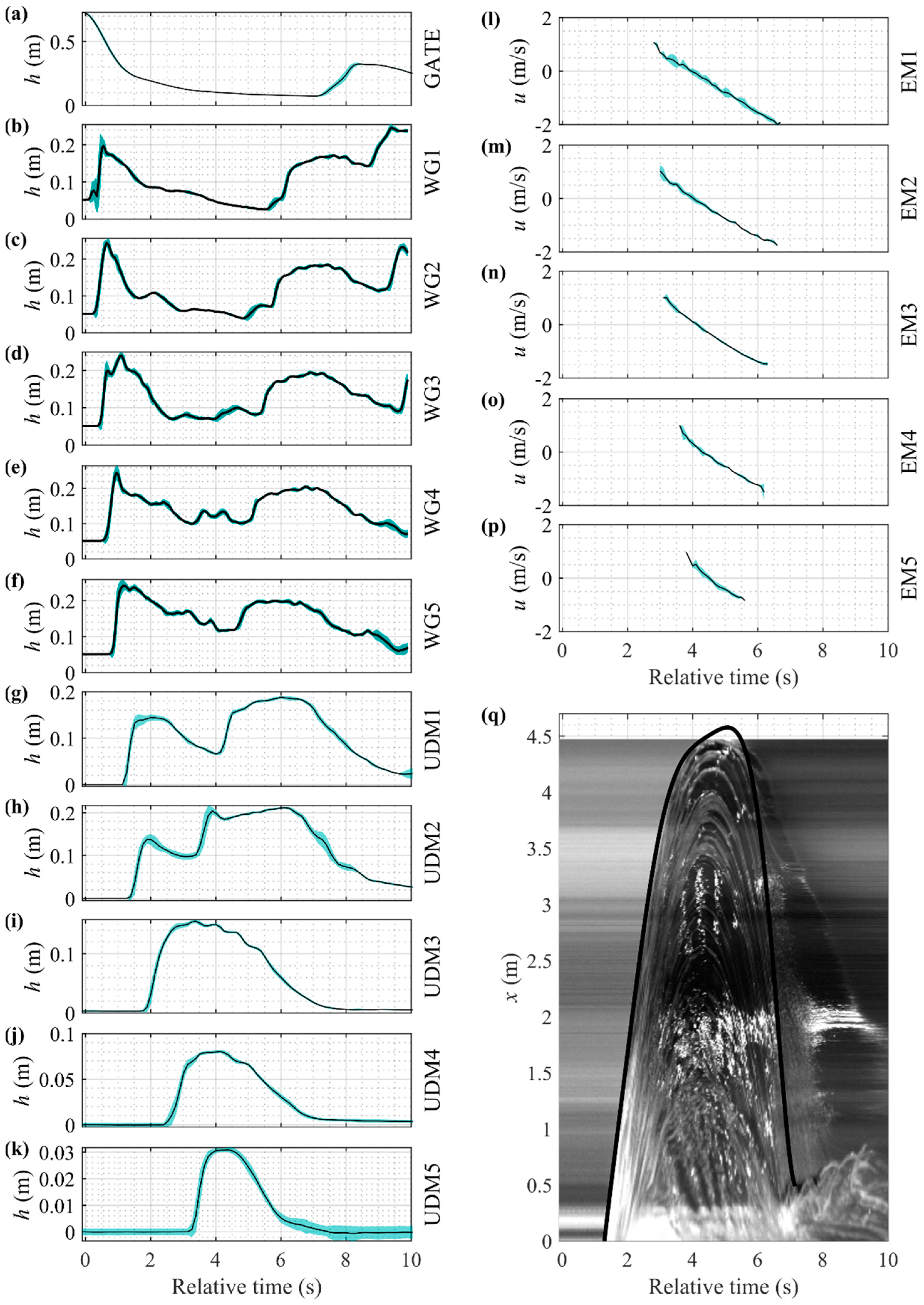
Jmse 11 00079 g002
Figure 3. Ensemble-averaged time series (solid line) and +/−1 standard deviation (shaded area) from the 10 hydrodynamic test repetitions for water level (ak) and velocity (lp), and a typical cross-shore time stack and corresponding runup curve (note that the runup exceeded the field of view and was fit by cubic spline) (q).
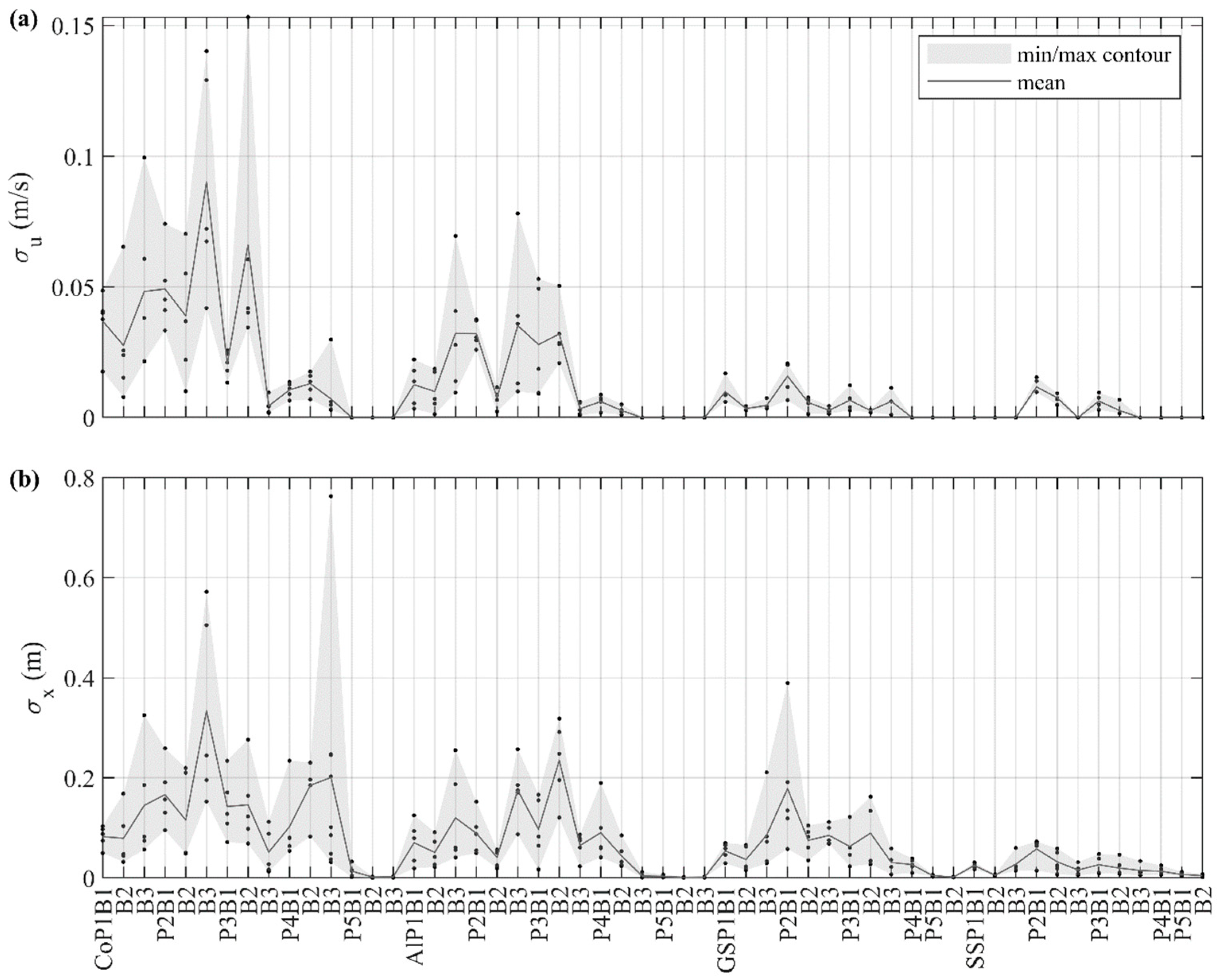
Jmse 11 00079 g003
Figure 4. Standard deviations of velocity (a) and distance travelled (b) for each scenario. Black circles indicate the standard deviations for individual runs.
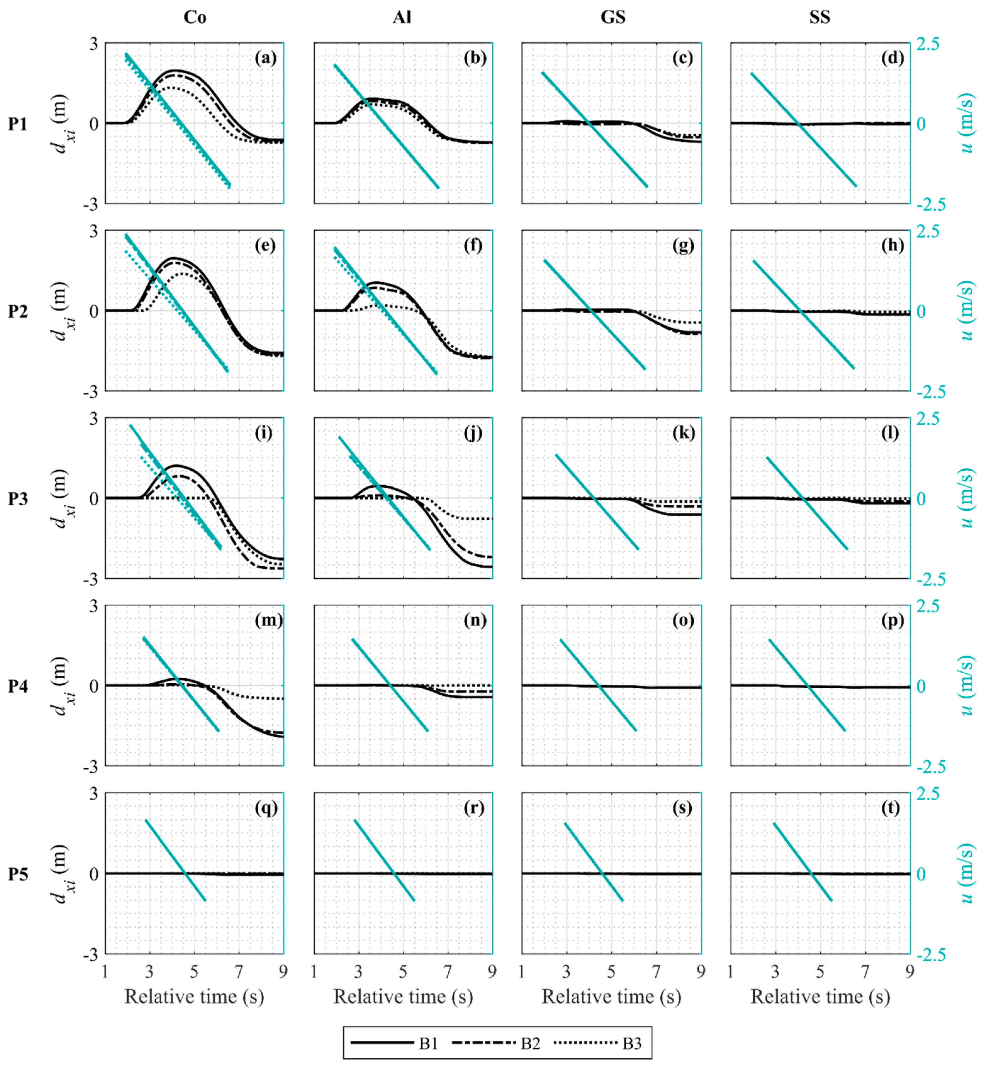
Jmse 11 00079 g004
Figure 5. Averaged distance travelled and averaged interpolated cross-shore flow velocity for each scenario tested. (a) CoP1. (b) AlP1. (c) GSP1. (d) SSP1. (e) CoP2. (f) AlP2. (g) GSP2. (h) SSP2. (i) CoP3. (j) AlP3. (k) GSP3. (l) SSP3. (m) CoP4. (n) AlP4. (o) GSP4. (p) SSP4. (q) CoP5. (r) AlP5. (s) GSP5. (t) SSP5.
Jmse 11 00079 g005
Figure 6. Example of hydrodynamics, object response, and moment for the AlP1B1 scenario. (a) Measured water depth, flow velocity and computed object velocity. (b) Measured object migration and estimated moment.
Jmse 11 00079 g006
Figure 7. (a) Moment—cross-shore flow velocity relationship; observed data (gray circles), Equation (23) fitted for each event (black lines) and Equation (23) with mean coefficients c1m, c2m, and c3m (blue line). (b) Comparison between observed and predicted moment dimensionless group using Equation (23) with mean coefficients.
Jmse 11 00079 g007
Figure 8. Uprush cross-shore distance travelled—moment relationship and coefficients. Lines correspond to Equation (24) fitted for each averaged event for objects with concrete (a) and aluminum (c) densities. Markers indicate the coefficients k1, k2, and k3, of Equation (24) varying as a function of the scenario and for objects with concrete (b) and aluminum (d) densities.
Jmse 11 00079 g008
Figure 9. Backwash cross-shore distance travelled—moment relationship and coefficients. Lines correspond to Equation (24) fitted for each averaged event for objects with concrete (a) and aluminum (c) densities. Markers indicate the coefficients k1, k2, and k3, of Equation (24) (e) varying as a function of the scenario and for objects with concrete (b) and aluminum (d,f) densities.
Jmse 11 00079 g009
Figure 10. Map representing the Delmarva region (a) and a picture of the field site (b). Significant wave height (c), peak wave period (d) and mean wave direction (e) during the study. Direction units are degrees from true North, increasing clockwise, with North as 0° and East as 90°. Solid straight line in panel E indicates the shore normal direction (133°). Shaded time windows represent Hurricane Florence and the force balance munition testing time, respectively. Data are provided by the NOAA National Data Buoy Center; station 44089—Wallops Island (VA).
Jmse 11 00079 g010
Figure 11. Field setup. (a) 2D map of deployed infrastructure and instrumentation in the local reference system. (b) Schematic of a generic instrumentation station (stations 1–9 only) with pipe and sensors configuration. (c) Photo of the frame scaffolding pipes holding instrumentation (offshore into page).
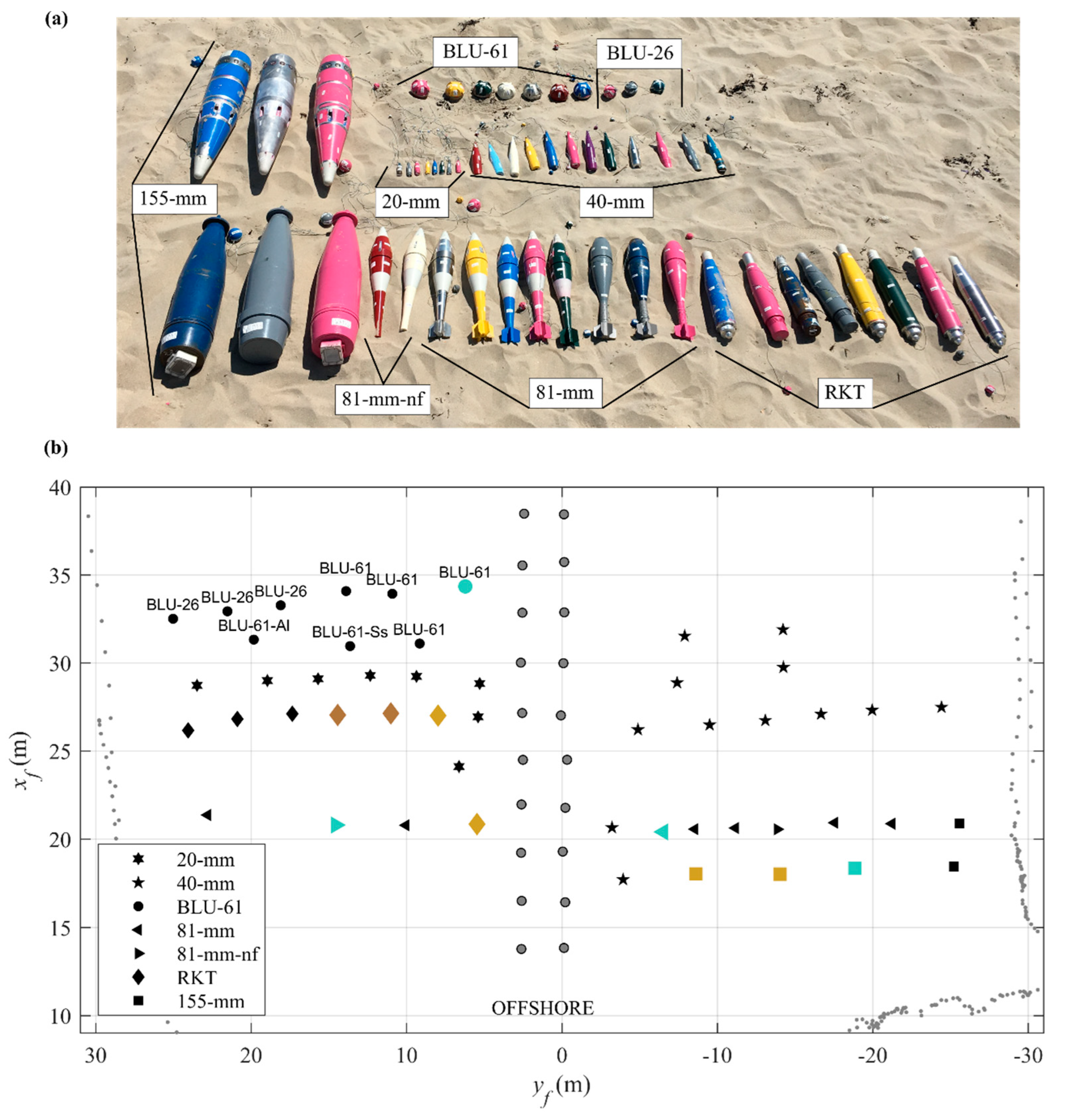
Jmse 11 00079 g011
Figure 12. (a) Munition variety used during the study for both long term and force analysis munitions. (b) Long term munition initial deployment. Color-coding is related to munition instrumentation, brown = PT; turquoise = IMU; gold = IMU and PT and black = not instrumented.
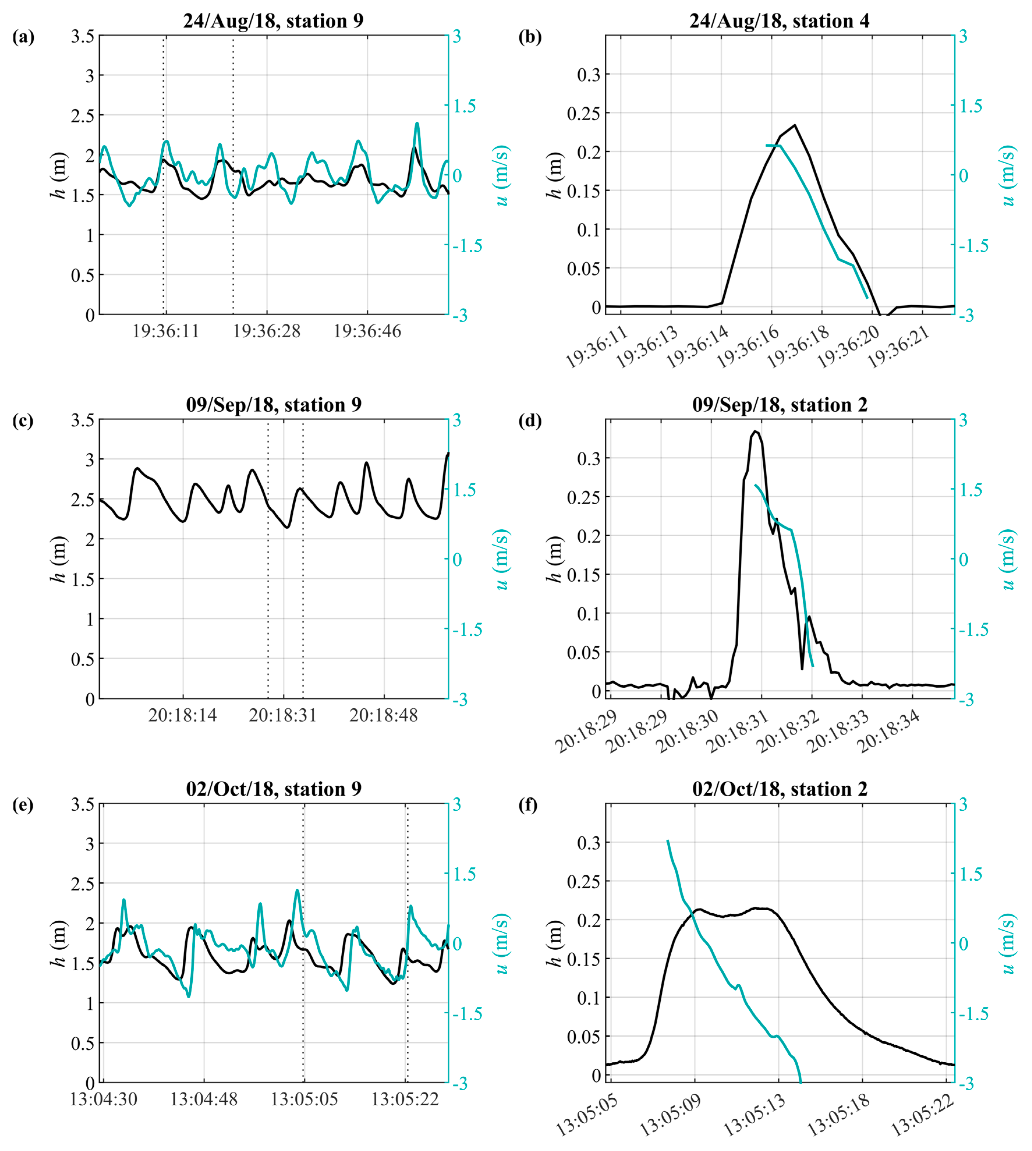
Jmse 11 00079 g012
Figure 13. Example hydrodynamics, water depths and near-bed cross-shore velocities observed during the experiment in calm conditions (a,b), storm event (c,d) and during the period the force balance analysis was carried out (e,f).
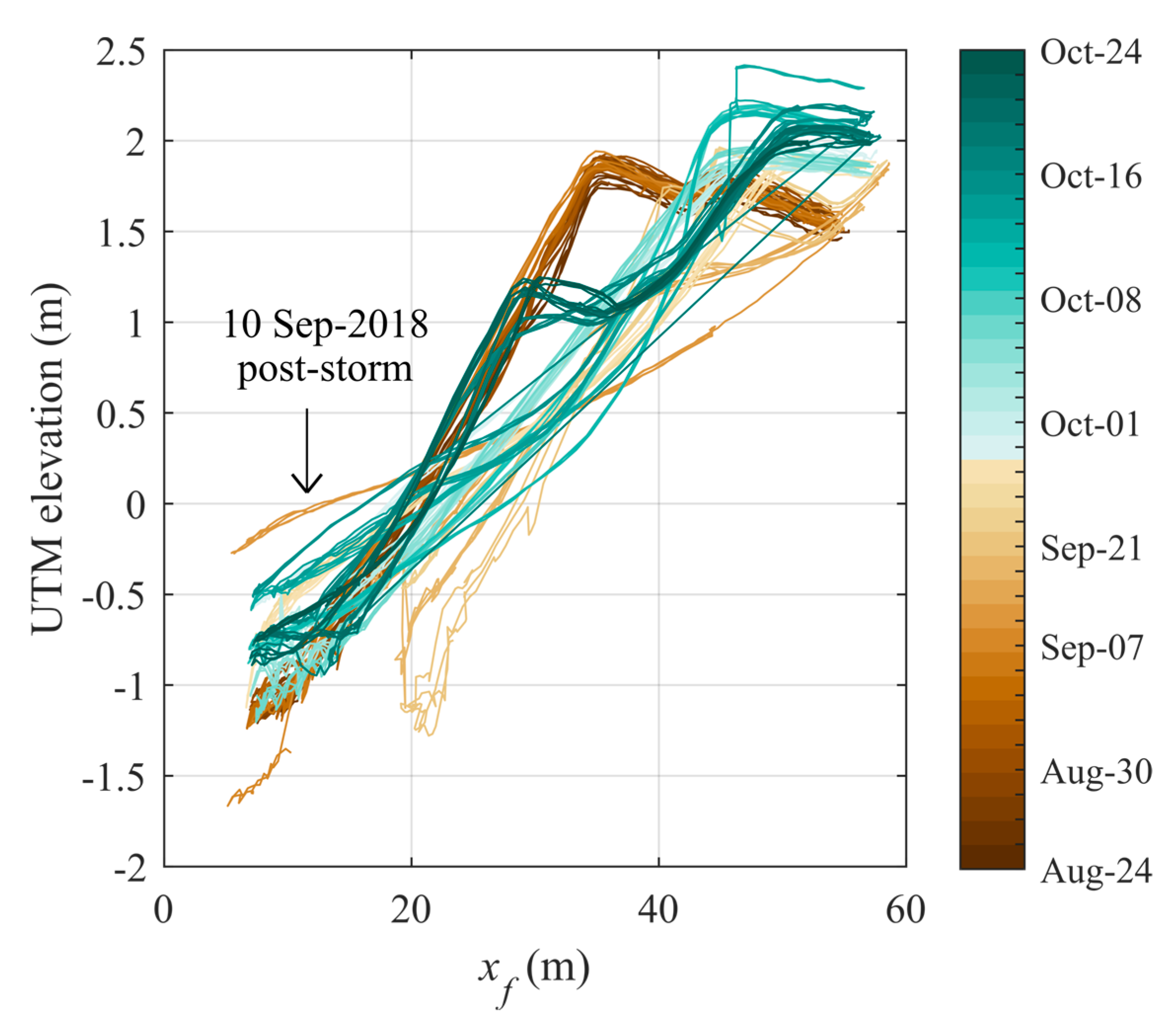
Jmse 11 00079 g013
Figure 14. Beach profile evolution over the experiment duration. The profiles are the transect surveyed on the left (north) side of the frame looking seaward (yf approximately −5 m).
Jmse 11 00079 g014
Figure 15. Long term deployed munitions observations. (a) Migration distances in xf and yf from initial (xf,yf) position. (b,c) Rate of change of the dimensionless burial depth as a function of the rate of change of the dimensionless beach morphology change for munitions that remained in place (b) or moved (c). Migration distances and rate of change of burial depth of each symbol are evaluated as the difference between the position or the burial depth between adjacent surveys. The color scheme is associated with munition diameter with darker colors for larger munition calibers.
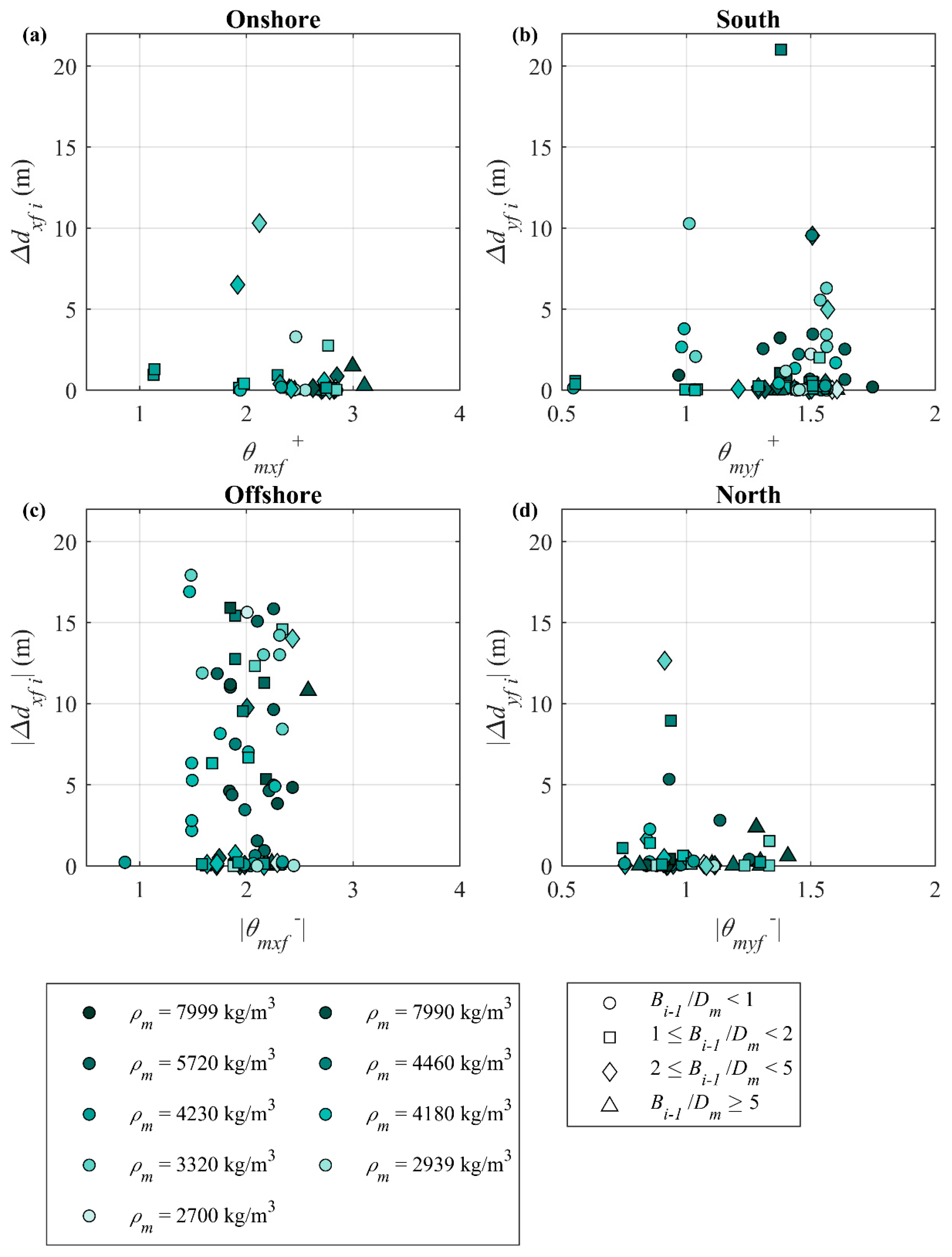
Jmse 11 00079 g015
Figure 16. Long term field deployed munition observations. Comparison between migration distance components and object mobility number: (a) Offshore, (b) South, (c) Offshore, (d) North. Markers are color coded to indicate munition density. Marker symbols indicate the initial dimensionless burial depth.
Jmse 11 00079 g016
Figure 17. Mobility of the instrumented RKT deployed at xf = 27.1 m and yf = 8.2 m on 24 August. (a) IMU cross-shore trajectory of relative distance (solid black line) and cross-shore locations of measuring stations 4–8 (circles, the color scheme follows panel b legend) referenced to 27.1 m. (b) Water depth measurements (RBR) at stations 4–8 and at the munition location (PT). (c) Cross-shore flow velocities relative to stations 4–8 (Vectrino and JFE).
Jmse 11 00079 g017
Figure 18. Example of hydrodynamics and munition (81-mm-nf) response to a swash event. (a) Measured water level and flow velocity at station 2. (b) IMU derived munition migration and final GPS munition position. (c) Frames of the munition response at times T1–T9 collected by the UC video imagery.
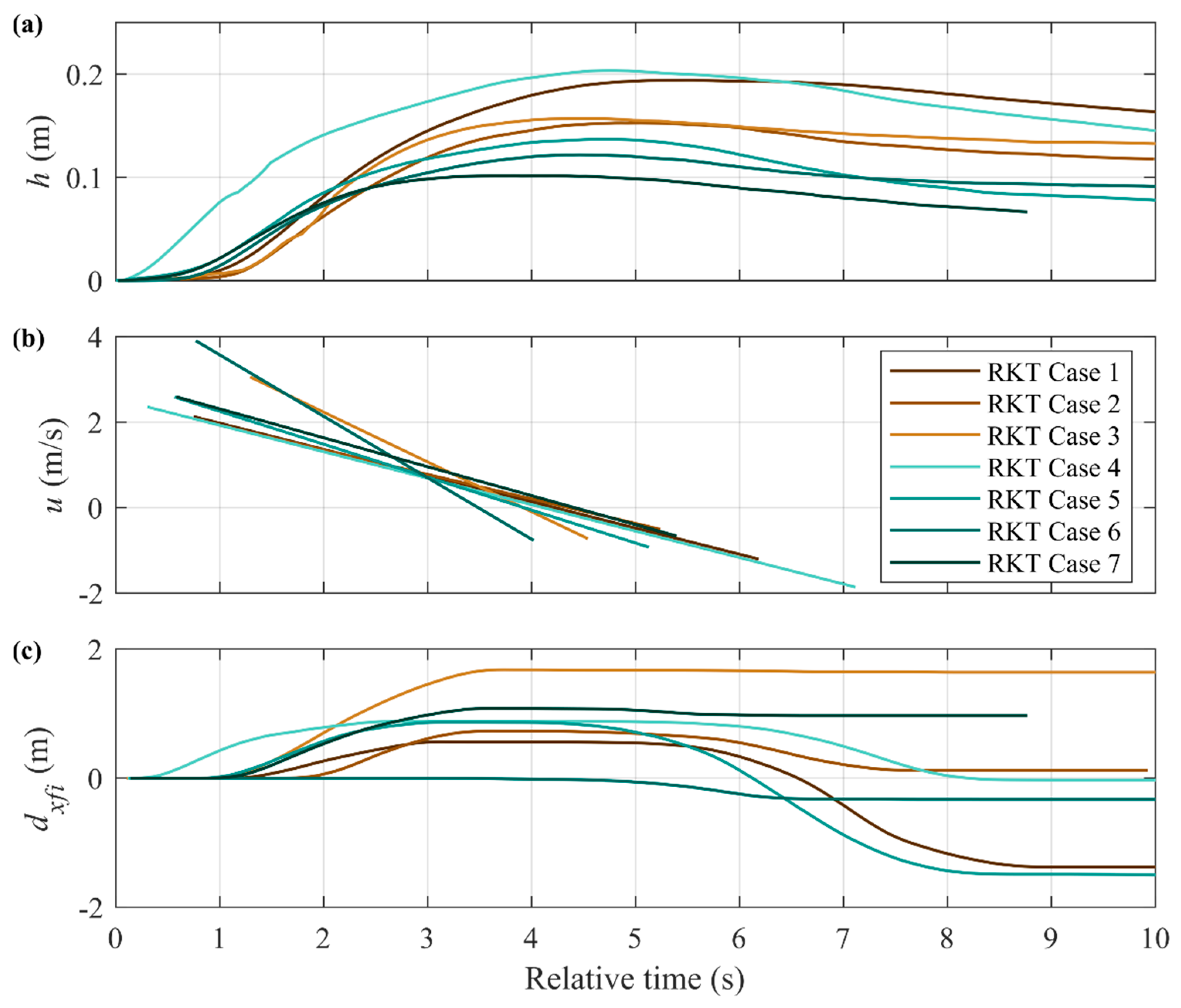
Jmse 11 00079 g018
Figure 19. RKT single swash event field responses. (a) Measured water level at station 2. (b) Flow velocity at station 2 (c) IMU derived munition migration and final GPS munition position.
Jmse 11 00079 g019
Figure 20. Comparison between the flume and field cross-shore distance travelled and moment dimensionless groups for uprush (a) and backwash (b). Only field munitions that were mobilized are reported in this figure.
Jmse 11 00079 g020
Table 1. Drag, lift, added mass and friction coefficients adopted by several studies investigating the mobility of objects on a sloping bed.
CoefficientStudyValue
CdLuccio, 1998 [3]1.000
Nott, 2003 [10]2.000
Imamura et al., 2008 [7]1.050
Nandasena and Tanaka, 2013 [8]1.950
ClLuccio, 1998 [3]1.000
Nott, 2003 [10]0.178
Imamura et al., 2008 [7]-
Nandasena and Tanaka, 2013 [8]0.178
CmLuccio, 1998 [3]1.000
Nott, 2003 [10]2.000
Imamura et al., 2008 [7]1.670
Nandasena and Tanaka, 2013 [8]1.000
CfLuccio, 1998 [3]0.1, 0.4 (smooth, rough bed)
Nott, 2003 [10]0.875
Imamura et al., 2008Variable
Nandasena and Tanaka, 2013Variable
Table 2. Specifications of the objects deployed during the laboratory study and the options of initial position and burial depth.
Initial PositionInitial Burial DepthDensity
Acronymxi (m)AcronymBi/DmAcronymρm (kg/m3)
P11.4B10Co (concrete)1800
P22.0B20.3Al (aluminum)2700
P32.6GS (galvanized steel shell)4200
P43.2B30.5SS (stainless steel)7700
P53.8
Table 3. Scenarios tested during the laboratory study (56 in total). Acronyms are defined in Table 2.
CoAlGSSS
P1B1 B2 B3B1 B2 B3B1 B2 B3B1 B2 B3
P2B1 B2 B3B1 B2 B3B1 B2 B3B1 B2 B3
P3B1 B2 B3B1 B2 B3B1 B2 B3B1 B2 B3
P4B1 B2 B3B1 B2 B3B1B1
P5B1 B2 B3B1 B2 B3B1 B2B1 B2
Table 4. Statistics of the coefficients c1, c2, and c3 (Equation (23)).
MinimumMaximumMeanStandard Deviation
c10.00010.00210.00110.0004
c2−0.05420.0289−0.00480.0138
c3−2.16780.9574−0.77020.5749
Table 5. Coefficients k1, k2, and k3 (Equation (24)) obtained for different scenarios.
CoAlGSSS
k1k2k3k1k2k3k1k2k3
UBUBUBUBUBUBUBUBUB
P1B10.0004−0.0004−0.0363−0.03020.5170−0.0028−0.00250.0001−0.0058−0.02840.22950.0010 −0.0034 0.0043 0.0047
B20.00060.0010−0.0382−0.04580.4589−0.0232−0.00250.0012−0.0079−0.03890.2030−0.0128
B30.00080.0019−0.0377−0.05330.3310−0.03020.00020.0014−0.0246−0.03720.1482−0.0537
P2B10.00070.0010−0.0418−0.05280.5320−0.00420.00160.0017−0.0455−0.05680.2892−0.0084 −0.0043 0.0023 0.0019
B20.00100.0014−0.0434−0.05610.4603−0.02840.00080.0016−0.0332−0.04980.2082−0.0230 −0.0031 −0.0016 0.0029
B30.00420.0016−0.0679−0.05070.2756−0.03380.00120.0002−0.0141−0.01940.0282−0.0245
P3B10.0009−0.0011−0.0354−0.03640.3219−0.01360.00100.0009−0.0263−0.04810.1150−0.0191
B20.00110.0007−0.0338−0.05080.2010−0.0272 −0.0013 −0.0192 −0.0167
B3 −0.0028 0.0026 0.0027
P4B10.00050.0001−0.0130−0.02180.0603−0.0105
B2 −0.0013 −0.0096 −0.0106
B3
P5B1 No motion observed
B2
B3
Table 6. Specifications of long term deployed munitions and force analysis munitions and physical munition parameters.
Long Term MunitionsForce Analysis Munitions
Munition IDDm (m)Lm (m)ρm (kg.m3)No
Sensors
SensorsMunition IDDateSensorsCases
20-mm0.020.07579908-RKT2 OctoberIMU, PT7
40-mm0.0400.200572012-
BLU-260.0650.06529393-BLU-613 OctoberIMU7
BLU-610.0990.099446031
BLU-61-Ss0.0990.09979991-81-mm9 OctoberIMU13
BLU-61-Al0.0990.09927001-
81-mm0.0810.48141806181-mm-nf4 OctoberIMU7
81-mm-nf0.0810.481418011
RKT0.0700.405332034155-mm10 OctoberIMU, PH, PT24
155-mm0.1550.754423023
TOT 4010TOT 58
Disclaimer/Publisher’s Note: The statements, opinions and data contained in all publications are solely those of the individual author(s) and contributor(s) and not of MDPI and/or the editor(s). MDPI and/or the editor(s) disclaim responsibility for any injury to people or property resulting from any ideas, methods, instructions or products referred to in the content.

