Digital Filter Design for Force Signals from Eulerian–Lagrangian Analyses of Wave Impact on Bridges

Abstract

Finite element (FE) models that simulate wave–superstructure interactions with the coupled Eulerian–Lagrangian (CEL) technique provide a viable and economical solution to estimate wave impact forces on bridge superstructures. One of the main drawbacks of CEL FE models is that they produce solutions distorted by numerical artifacts with very high frequencies that make it difficult to quantify the magnitude of hydrodynamic forces on superstructures. This paper investigated digital filter parameters for horizontal forces extracted from CEL FE models. The optimal filter configuration was evaluated by comparing unfiltered and filtered horizontal force signals with experimentally measured values from a reduced-scale superstructure specimen tested at the O.H. Hinsdale Wave Research Laboratory at Oregon State University. It was found that digital filters with cutoff frequencies below the fundamental frequency of the superstructure produced the best results and that optimizing Eulerian–Lagrangian surface interactions significantly improved the quality of the calculated force signals.

1. Introduction

Bridges, a critical component of transportation networks in coastal areas, are vulnerable to extreme storm surge and wave impacts caused by hurricane events. In recent decades, hurricanes Katrina (2005) and Ivan (2004) had catastrophic effects on bridge infrastructures located along the Louisiana and Mississippi coasts. The cost of repairing and replacing bridges damaged during hurricanes Katrina and Ivan was estimated to exceed $1 billion [1]. Large hurricane winds cause storm surges, which raise the water level and create interactions between ocean waves and bridge superstructures. Fluid–structure interactions occur in two scenarios: (i) superstructure submergence or (ii) waves slamming against a superstructure. The process of reconstructing or retrofitting bridges to better withstand extreme hurricanes demands a reliable estimation of hydrodynamic forces acting on the bridge superstructure. Large-scale experimentation on bridge structures is not possible in flume facilities [2,3,4], making it necessary to develop numerical simulation techniques to enhance our knowledge of the hydrodynamic wave forces acting on these structures. Complex numerical simulations to calculate forces resulting from wave–superstructure interactions during extreme hurricane events are sensitive to modeling parameters and computationally expensive.

The large computational cost of complex models used to simulate fluid–structure interactions has motivated researchers to reduce computation time by using simplified models. Kerenyi et al. [5] developed a 3D FE six-girder model representing a strip of a bridge containing a rail and a gap. Lau et al. [6] calibrated numerical models to estimate the hydrodynamic wave forces on bridges based on experimental results from flume tests. The models included a bridge deck and supporting piers in order to account for substructure flexibility. They characterized the horizontal and vertical force histories as consisting of two parts: the impulsive phase, which included the peak force, and the slowly varying component, which included a slower varying force after the wave had passed the bridge. Bozorgnia [7] conducted a suite of 2D and 3D numerical models and compared their measurements with the experimental models developed by Bradner et al. [8]. It was found that the peak magnitude of the resulting hydrodynamic forces was heavily dependent on element size and the number of time increments defined in each step. Yim and Azadbakht [9] estimated the horizontal and vertical forces resulting from tsunami wave loads on the US Highway-101 Spencer Creek Bridge at Newport, Oregon. A range of different mesh sizes and time steps were implemented in their numerical models to achieve convergence and reduce excessive computational costs.

Past research [10,11,12,13,14,15,16] has shown that the Coupled Eulerian–Lagrangian (CEL) method is a reliable technique that enables the modeling of fluid–structure interactions due to wave impacts by simultaneously considering the behavior Lagrangian and Eulerian domains [17,18,19].

Montoya et al. [20] and Majlesi et al. [21] developed 3D FE models using the Coupled Eulerian–Lagrangian (CEL) method to estimate vertical and horizontal hydrodynamic forces on coastal bridges over Biloxi Bay MS (U.S. 90) and Escambia Bay FL (I-10). Their research showed that the calculated vertical forces exceeded the weight of the deck and that including the superstructure flexibility in the analysis of these bridges significantly altered the numerical stability and magnitude of the force signals. Force signals at the substructure–superstructure interface extracted from CEL numerical models included high-frequency oscillations that did not represent the true physics of wave–superstructure interactions [9,17,18,20,22,23,24,25,26,27,28,29,30,31]. Although major improvements have been observed in the FE modeling of wave–superstructure interactions, the source of the abovementioned oscillations remains poorly understood.

In a number of past studies [9,18,22,23,24,25,27,32], digital filtering has been used to remove numerical artifacts from force time histories. Azadbakht and Yim [28] used a low-pass filter to remove the unfavorable spikes in their resulting force time histories. Xiang and Istrati [24] used a Butterworth filter with a cutoff frequency of 30 Hz for both experimental and numerical force signals to remove the influence of structural dynamics from the computed forces. The filter design that they used was the same throughout their parametric study, neglecting the first mode frequency of superstructures with different dimensions. In another study, Xiang et al. [22] proposed a digital filter design based on the fast Fourier transforms (FFTs) of the vertical and horizontal force signals. Initially, they found the frequencies of the governing modes and developed a digital filter that eliminated the fundamental frequency of the structure. A low-pass Butterworth filter with a range of cutoff frequencies was used to find the optimal digital filter. Eventually, they chose a digital filter with a cutoff frequency lower than the fundamental frequency of a bridge structure based on the premise that the mass of a wave interacts with a deck, increasing the effective mass of the deck and decreasing the fundamental frequency of the bridge.

Tuning the modeling parameters in a CEL solver requires a parametric study and comparison with the results of an experimental model [33,34,35]. The simulations performed for this paper were based on numerical models of a reduced-scale superstructure specimen subjected to wave impacts in the O.H. Hinsdale Wave Research Laboratory at Oregon State University by Bradner et al. [36].

The study consisted of the following steps, illustrated in Figure 1. An ABAQUS CEL numerical model with non-optimized modeling parameters was developed and used to calculate forces at the superstructure–substructure interface. Subsequently, different digital filter designs were applied to the force signals to evaluate the performance of the filter in removing unwanted numerical artifacts. In the next step, filtered signals were quantitatively and qualitatively compared with those from a CEL numerical model with optimized modeling parameters. This paper illustrates two different methodologies (tuning and filtering) to reduce numerical artifacts and computational time and to increase the accuracy of the predicted outputs.

2. Numerical Model

The dimensions of the finite element model, summarized in

Table 1. Properties of the bridge superstructure model (1:5) and prototype.

Parameters	Model (1:5)	Prototype (1:1)
Span length, S	3.45 m	17.27 m
Width, H	1.94 m	9.70 m
Girder height	0.23 m	1.14 m
Girder Spacing (CL to CL)	0.37 m	1.83 m
Deck thickness	0.05 m	0.25 m
Overall height	0.28 m	1.40 m
Span weight	19.0 kN	2375 kN
Span mass	1.94 t	242 t

, were based on a 1:5 scale physical model of the I-10 Bridge over Escambia Bay bridge tested at Oregon State University. The numerical model consisted of six reduced-scale AASHTO (American Association of State Highway and Transportation Officials) Type III girders and a bridge deck.

The ABAQUS implementation [37] of the CEL technique employed in this study can only be used in conjunction with an explicit solver, and the accuracy of the results is highly dependent on the choice of explicit analysis parameters. The loading sequence of the numerical model had two steps. The gravity load was applied to the numerical model in the first step (t = 0 to t = 10 s), and the wave forces were applied in the second (t = 10 to t = 19 s). Both steps were analyzed using the dynamic/explicit method with a maximum time increment of 1 × 10⁻⁶ s. The material model parameters utilized for concrete and water instances were the same as those used by Majlesi et al. [30]. The air trapped between the girders was ignored because only the horizontal hydrodynamic force was used in the calibration of the model and the evaluation of the force signal, and the horizontal force was not sensitive to air entrapment between girders [28].

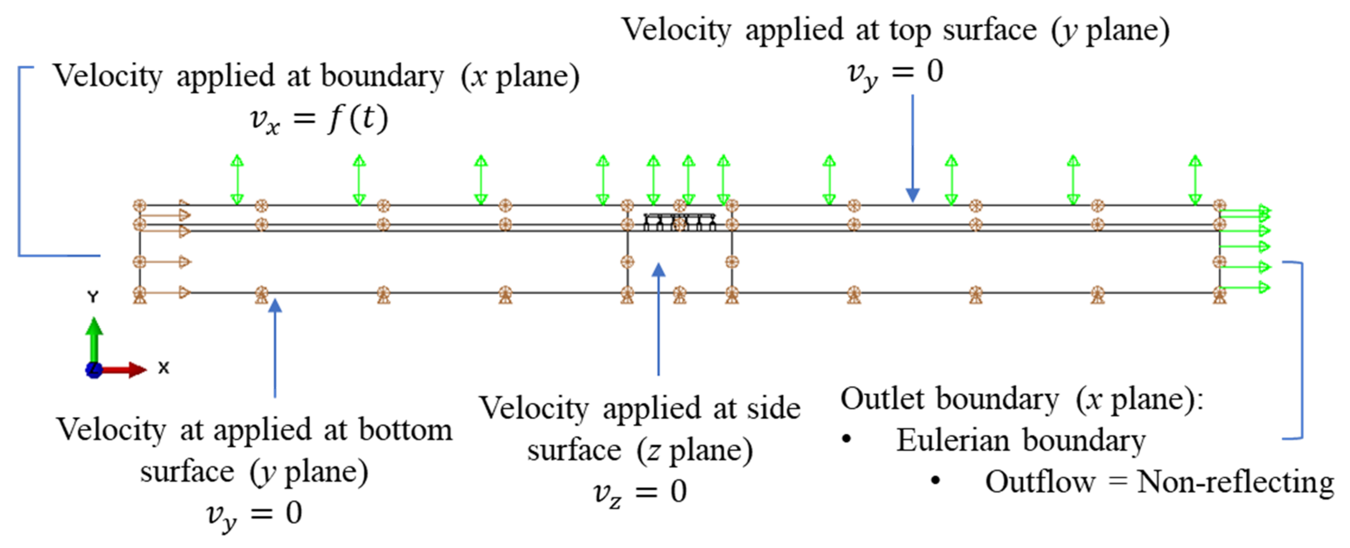
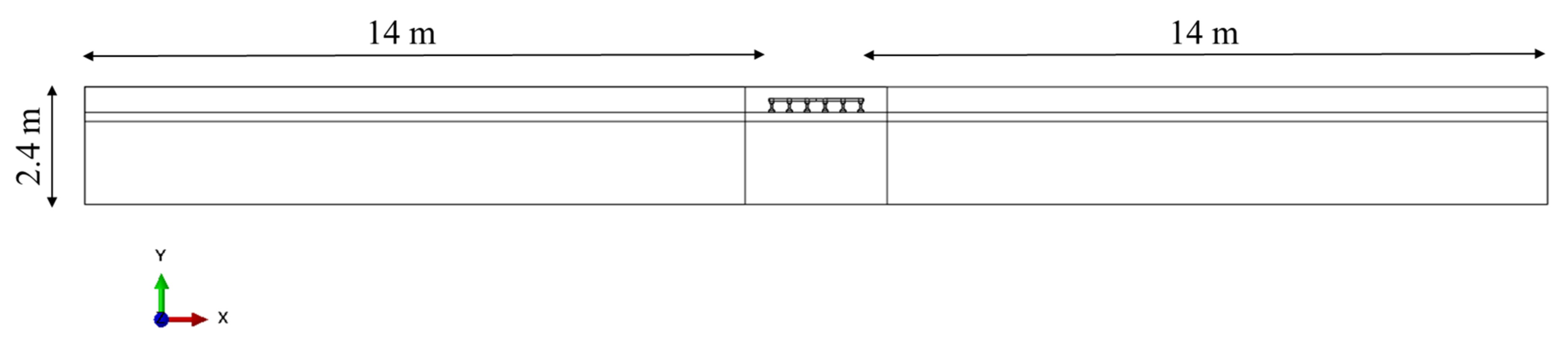
2.1. Wave Flume

A crucial aspect of CEL models is the precise modeling of the wave introduced in the Eulerian domain. In a previous study, Shahriar et al. [38] applied the Lagrangian-plus remap technique to generate periodic waves in an Eulerian domain where the superstructure was located using ABAQUS. Although the wave height and period of the generated waves were slightly different from the analytical values, Fourier analysis proved that the wave inconsistency observed in the first time increments decreased as the wave traveled through the numerical flume. The recommendations provided by Shahriar et al. [38] were implemented for modelling waves in this paper. The appropriate loading and boundary conditions reacting on each side of the 3D wave numerical flume are shown in Figure 2. Waves were produced by applying a velocity profile $v_x$ at an inlet located at the left boundary of the Eulerian domain [38].

Periodic waves are characterized by three independent variables, which are and initial water depth ($h$), wave height ($H$), and wave period ($T$). For a wave with a relatively small amplitude, the surface elevation, $n$, can be defined as $n=-\mathrm{asin}\left(kx-\omega t\right)$, where $\omega =2\pi /T$ is the circular frequency, $a=H/2$ is the wave amplitude, and $k=2\pi /\gamma$, is the number of the wave. In linear wave maker theory [39], the displacement of a wavemaker is defined as:

$$\xi \left(t\right)=-{\xi }_0\cos \left(\omega t\right)$$

(1)

where ${\xi }_0=\frac{a{n}_1}{\mathit{tanh}\left(kh\right)}$, $n_1=\frac{1}{2}\left(1+\frac{2kh}{\sin \left(2kh\right)}\right)$, and $k$ is the wave number, which can be determined from the dispersion relation provided by Lamb [40] as:

$${\omega }^2=gktanh\left(kh\right)$$

(2)

Equation (2) represents the solution obtained with first-order wave theory. Madsen [41] showed that by utilizing the wavemaker motion, an unwanted free second harmonic will be produced that distorts the desired wave from the analytical solution. The free surface is described by Equations (3)–(5):

$$n=-\mathrm{asin}\left(k_{p}x-\omega t\right)-a_{2p}cos2\left(k_{p}x-\omega t\right)+a_{2f}\cos \left(k_{f}x-2\omega t\right)$$

(3)

$$a_{2p}=\frac{k_p{a}^2}{4}\frac{\left\{2+\cosh 2\left(k_{p}h\right)\right\}\cosh \left(k_{p}h\right)}{{\sinh }^3\left(k_{p}h\right)}$$

(4)

$$a_{2f}=\frac{a^{2}coth\left(k_{p}h\right)}{2h}\left(\frac{3}{4{\sinh }^2\left(k_{p}h\right)}-\frac{n_1}{2}\right)\frac{tanh\left(k_{f}h\right)}{n_2}$$

(5)

where $n_2=\frac{1}{2}\left(1+\frac{2k_{f}h}{sinh2\left(k_{f}h\right)}\right)$. In Equation (5), $k_p=k$ and $k_f$ are the wave numbers of the main and free wave, respectively. The 1st term of Equation (5) is the first-order wave module, which represents the primary wave, and the second term is defined as the Stoke second-order wave, which has a celerity equal to the desired wave. The third term is the second-order free wave, which is defined as:

$$4{\omega }^2=g{k}_{f}tanh\left(k_{f}h\right)$$

(6)

The main characteristics of the waves interacting with the physical model tested at Oregon State University are shown in

Table 2. Wave parameters of the numerical model.

Parameters	Magnitude
Initial water depth, h	1.9 m
Wave height, H	0.5 m
Wave period, T	2.5 s
Domain Length, L	30 m

. The wave parameters implemented in the numerical model were the same as those used in the test of the physical model, where the superstructure elevation left no gap between the bottom of the girders and the water underneath.

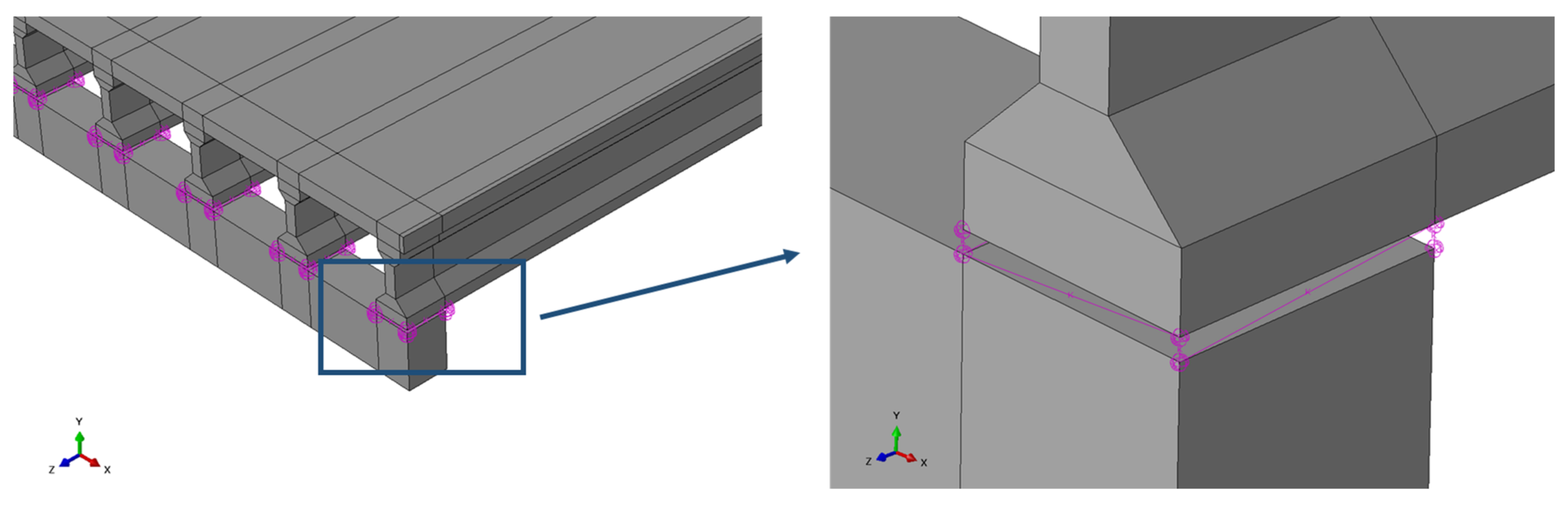
2.2. Surface Contact Interaction Definition

Contact between the Eulerian and Lagrangian elements was defined using general contact interaction in ABAQUS, which implements the penalty contact method that resists node-to-face and edge-to-edge contact penetrations [42]. This type of contact interaction definition is more flexible than the kinematic contact interaction used in dynamic problems. To ease the extraction of the horizontal forces acting on the superstructure, multiple springs in the X, Y and Z directions were added to connect the bent cap and the superstructure, as shown in Figure 3. It was found in a previous study [30] that using springs instead of a tied connection produced more accurate estimates of the hydrodynamic forces recorded in a physical model.

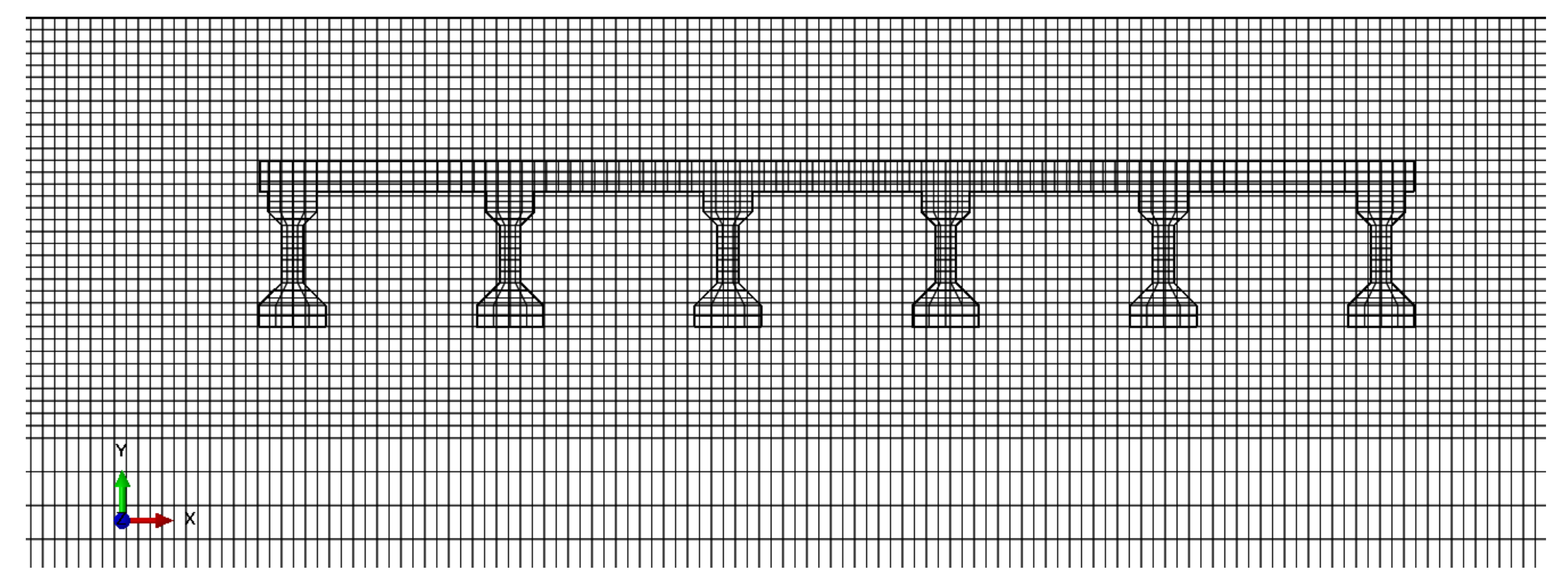
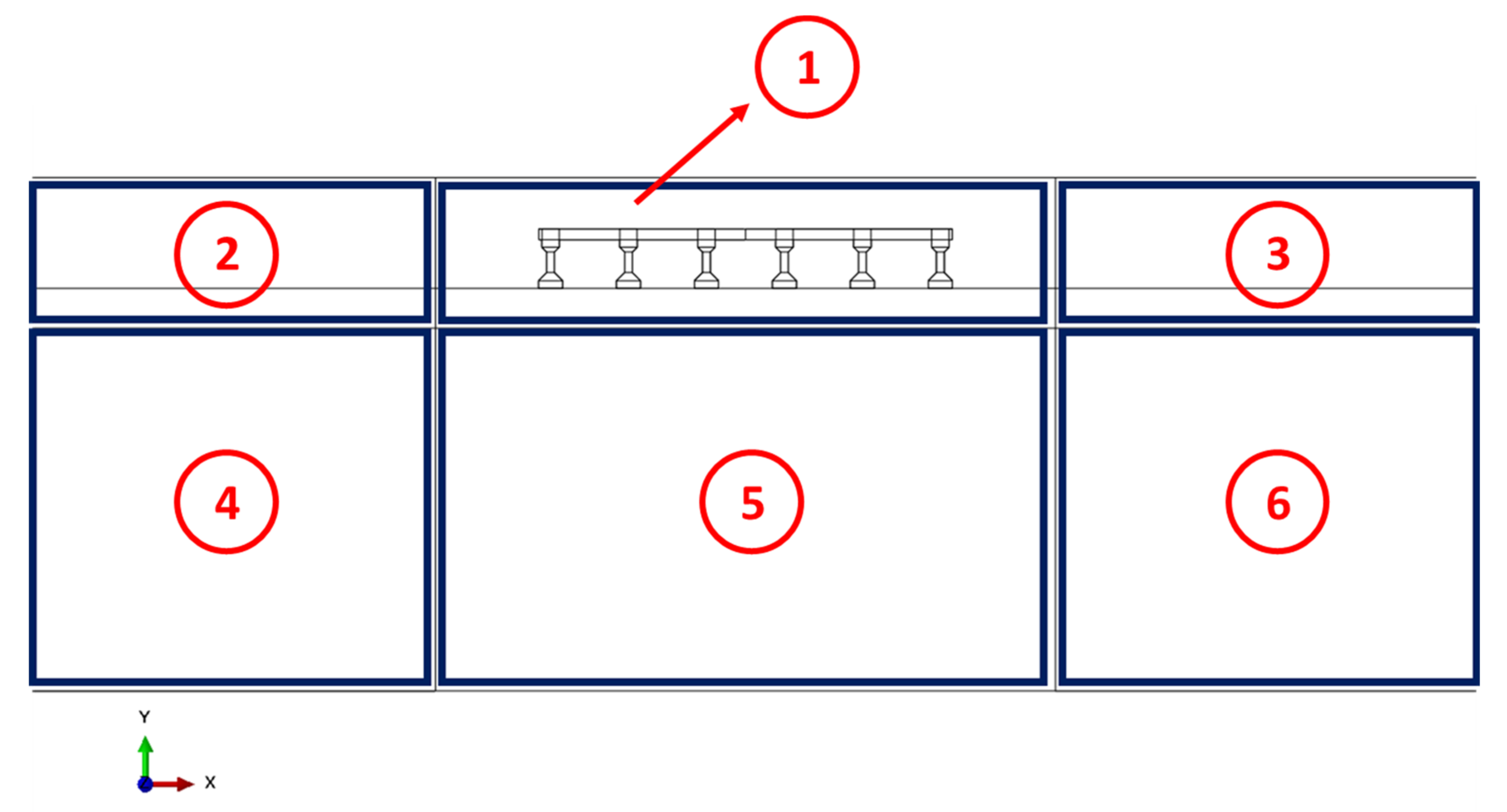
2.3. Meshing

Hexahedron solid elements (8-noded) were used to mesh the Eulerian and Lagrangian (superstructure and cap) instances. The overall number of Lagrangian and Eulerian elements in the models was approximately 1,320,000. A cross-section illustrating the mesh in the zone where wave–superstructure interactions occur is presented in Figure 4. The dimensions of the Eulerian domain and the location of the bridge superstructure are shown in Figure 5. The superstructure was placed at the center of the Eulerian domain because the study developed by Shahriar et al. [38] concluded that the waves most accurately matched the analytical solution at this location.

The numerical models had 6 different regions with different mesh sizes. The mesh size was smallest at region 1 and larger at the remaining regions. The element sizes for each of these regions are shown Figure 6 and

Table 3. Eulerian domain mesh sizes.

Mesh Size (cm)
Region 1		Regions 2 and 3		Regions 4 and 6		Region 5
Δx	Δy	Δx	Δy	Δx	Δy	Δx	Δy
2.0	2.0	11.2	2.0	11.2	5.6	2.0	5.6

. A mesh sensitivity study was performed to find the most efficient element dimensions in region 1, where the fluid–structure interactions took place.

2.4. Hourglass Control Parameters in Eulerian and Lagrangian Mesh

Hourglass control, an important modeling parameter in the CEL element formulations considered in this study, introduces an artificial numerical stiffness to reduce mesh distortions caused by hourglass modes. In reduced integration elements, the linear portion of the incremental displacement (designated as the hourglass field) is used to compute the physical strain. Unwanted mesh distortion without any opposition occurs when the hourglass modes have been exceeded. ABAQUS has a range of different solutions to stop excessive hourglass distortions. In the element formulations assigned in this study, the following parameters could be varied: displacement hourglass scaling factor s, linear bulk viscosity scaling factor b₁, and the quadratic bulk viscosity scaling factor b₂. The Kelvin-type viscoelastic force-moment conjugates to the hourglass mode magnitude (q), which is implemented in explicit models using Equation (7):

$$Q=s\left[\left(1-\alpha \right)Kq+\alpha C\frac{dq}{dt}\right]$$

(7)

where Q is the force or moment related to q, K is the hourglass stiffness, α represents the scaling factor that stabilizes viscous and elastic control, and C is the linear viscous coefficient. Throughout an explicit analysis, bulk viscosity creates artificial damping that can be changed at every analysis step. ABAQUS utilizes a linear bulk viscosity scaling factor b₁ to dampen oscillations of the element with the highest frequency in the stable time increment. As shown in Equation (8), the abovementioned damping introduces a bulk viscosity pressure where a linear correlation exists between pressure and the volumetric strain rate ${\dot{ϵ}}_{vol}$. Because a small number of elements experience extremely high velocity gradients, the quadratic viscosity scaling factor b₂ is introduced as an artificial pressure that distributes the shock wave over other elements and stops them from collapsing. The quadratic component of the pressure is shown in Equation (9).

$$p_{bv1}=b_1\rho c_d{L}_e{\dot{ϵ}}_{vol}$$

(8)

$$p_{bv2}=\rho {\left(b_2{L}_e{\dot{ϵ}}_{vol}\right)}^2$$

(9)

3. Parametric Study

The parametric study considered two models with different configurations. The modeling parameters that varied in the parametric study are presented in

Table 4. Modeling parameters for optimized and non-optimized FE models.

Model	Mass Scale Factor	Damping (%)	Eulerian Domain					Lagrangian Domain
			Hourglass Control	α	s	b1	b2	Hourglass Control	α	s	b1	b2
1	1	0.0	Default	DV a	DV a	0.06	1.2	Default	DV a	DV a	0.06	1.2
2	50	4.0	Combined b	0.25	1	0.06	1.2	Combined b	0.25	1	0.06	1.2

DV ^a: Default value. Combined ^b: Combination of elastic and viscous hourglass control.

. Optimized (model 2) and non-optimized (model 1) CEL models were developed to show the difference between unfiltered force signals that contained numerical artifacts. In model 1, FE parameters that had been used in previous ABAQUS/explicit hydrodynamic simulations were implemented [43,44,45]. As is shown with greater detail in subsequent sections, large numerical artifacts were observed in the force signal calculated with model 1 during wave–superstructure interactions. The modeling parameters optimized for model 2 included damping, mass scale factor [46], hourglass control, and its dependent variables. Model 2 optimization was performed in a separate parametric study, and the optimal modeling parameter values are presented in Table 4. The choice of modeling parameters used in model 2 produced smoother interactions between the Lagrangian and Eulerian elements.

Given that one of the goals of the study was to show the difference that modeling parameter optimization caused in the force signal, all force signals calculated with model 1 were digitally filtered with a low-pass filter. The range of cutoff frequencies for the low-pass filter was defined based on the fundamental frequency of the model. A frequency analysis performed on the bridge superstructure showed that the first and second mode had frequencies of 27.4 and 30.8 Hz, respectively (Figure 7). Modal participation factors for the first 40 modes of the bridge superstructure were extracted, and cumulative values for each degree of freedom (DOF) are shown in Figure 8.

The parameters of the low-pass digital filter used in this study included the passband ripple, passband frequency, and stopband frequency, as shown in Figure 9. The filtered signal results presented in this paper for model 1 correspond to 21 different digital filters, where the passband ripple, passband and stopband frequency parameters were varied. Filter parameters had passband frequencies ranging from 1 to 30 Hz, stopband frequencies ranging from 5 to 35 Hz, and passband ripple ranging from 0.05 to 0.6. A set of low-pass digital filters with a passband ripple of 0.05 used in the study is shown in Figure 10.

4. Performance Metrics

In order to compare the numerical and experimental force signals, this study considered two performance metrics described below.

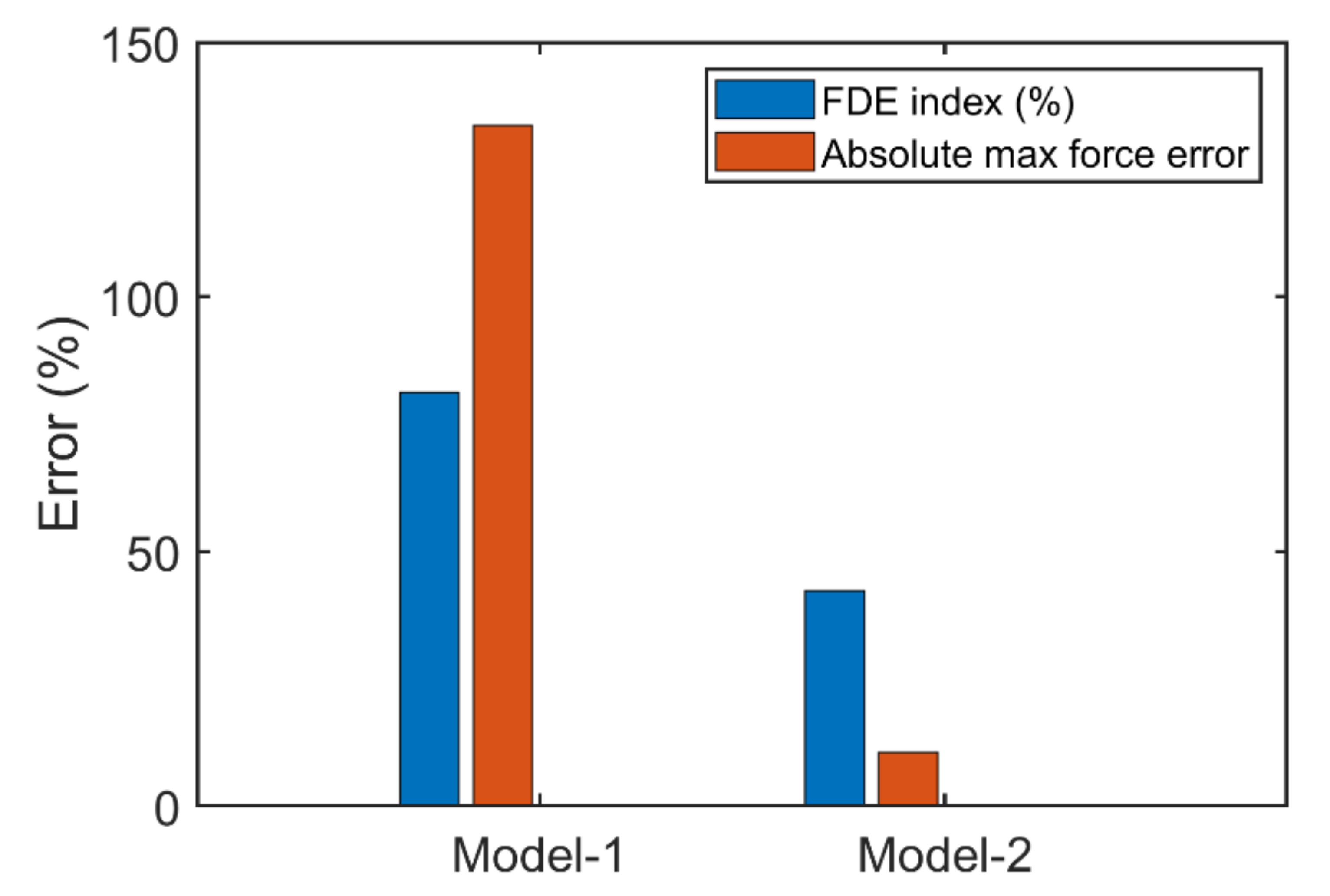
4.1. Frequency Domain Error (FDE) Index

A method developed by Dragovich and Lepage [47] was used to estimate the goodness of fit among different response signals. This method is called the frequency domain error (FDE) index and is calculated using the Fourier spectra of two waveforms. The FDE index accounts for both phase and amplitude differences between signals, and a higher FDE index value indicates a lower similarity between two compared signals. Assuming R_m, I_m, R_c and I_c as the real and imaginary components of the measured and computed signals, the following equation estimates the FDE index:

$$\mathrm{FDE}=\frac{{\displaystyle {\sum }_{i=f_1}^{f_2}}\sqrt{{\left(R_{m_i}-R_{c_i}\right)}^2+{\left(I_{m_i}-I_{c_i}\right)}^2}}{{\displaystyle {\sum }_{i=f_1}^{f_2}}\left(\sqrt{R_{m_i}^2+I_{m_i}^2}+\sqrt{R_{c_i}^2+I_{c_i}^2}\right)}$$

(10)

where f₁ is the initial Nyquist frequency for the sum and f₂ is the final Nyquist frequency for the sum.

Force signals from the two models were compared in two different ways. Filtered signals were compared with each other in terms of filter configuration (Figure 10) and with the unfiltered force signal from the optimized model.

4.2. Maximum Force Error

The maximum force calculated with the numerical models was compared with the maximum force recorded in the experimental model. The following equation was used:

$$Maximum force error=\frac{\left|F_{max}^n-F_{max}^e\right|}{F_{max}^e}$$

(11)

where $F_{max}^e$ is the maximum force resulting from the experimental model and $F_{max}^n$ is the maximum force resulting from the numerical model.

5. Results

The normalized horizontal force (with respect to the weight of the superstructure) calculated with the numerical models presented in Table 4 was compared in terms of the FDE index and the absolute maximum force error. The wave impact progression for model 1, calculated during the second step of the CEL simulation of model 1, is shown in Figure 11.

The execution times for the two models using the high-performance computers (ARC) at the University of Texas at San Antonio (Intel^© Xeon Gold 6248 @ 2.50 GHz × 20, San Antonio, TX, USA) are shown in

Table 5. Computational time (days).

Model	1	2
Computational time (days)	15	12

.

5.1. Model 1

The unfiltered normalized horizontal force signal for model 1 is shown in Figure 12. As shown in Figure 12, the FE model that was not optimized included major numerical artifacts throughout its signal. Regardless of this limitation, the numerical model was able to capture the overall trend of the experimental signal during wave impact between t = 17 s and t = 18 s. This observation provided assurance that applying digital filters with different configurations would likely reduce the numerical artifacts and produce a signal that would more closely qualitatively resemble the force signal from the experimental model.

The energy balance, defined as the summation of all energy components minus the work done by external forces, is an important indicator of the accuracy in explicit analyses [42]. Figure 13 shows the evolution of the energy output variables for model 1 over simulation time. It should be noted that the artificial strain energy in Figure 13 had a very small magnitude, so it coincided with the curve representing mass scaling work. The main cause of concern from this output was the increase in the magnitude of the total energy, particularly during wave impact. The absolute value of the total energy had significant increases at approximately t = 14.0 s and t = 18.0 s, which corresponded to the times when the first and second waves impacted the bridge. This suggests that additional energy was introduced into the CEL model during wave impact while Eulerian–Lagrangian interactions took place and that the magnitude of the change in total energy during wave impact was an indication of the significance of stabilization on the results [45]. Additionally, the numerical artifacts observed in the unfiltered force signal (Figure 12) further support the abovementioned hypothesis. Hence, the modeling parameters defined in model 2 were chosen to provide smoother wave–superstructure interactions.

To further understand the physics and frequency content of the numerical models, the fast Fourier transforms (FFTs) of unfiltered force signals from model 1 and similar models with different mass scale factors are presented in Figure 14. Amplitudes at frequencies lower than 1 Hz are attributed to the low-frequency component of the force signals, which are associated with the quasi-static component of the force signal [22]. In model 1, the FFT of the force signal had observable amplitudes at frequencies exceeding 50 Hz. The FFT amplitudes in Figure 14 indicate that the fundamental frequency of model 1 was 27.4 Hz, which was close the value calculated with the frequency analysis. CEL models were run with different mass scale factors, which affected the natural frequency of the models. The load cell signal from the experimental test was filtered with a low-pass filter with a cutoff frequency of 12.5 Hz [36], which was less than the natural frequency of the models with mass scale factors greater than 20. This was a limitation of the study that could not be resolved because even if the unfiltered signal was available, it was not possible to determine if high-frequency components of the experimental signal were attributable to wave impact or electrical noise.

The calculated force signal shown in Figure 12 was filtered using a range of different cutoff frequencies and passband ripples, as shown in Figure 15. The implemented digital filter was able to pass most frequencies unchanged, attenuating those in the cutoff range to small magnitudes. The filtered force signals presented in Figure 15 show that digital filtering was effective in removing the numerical artifacts from the calculated signals. A direct comparison between Figure 12 and Figure 15 shows that the force signals had more numerical artifacts prior to filtering and that, in most cases, the magnitude of the spikes was reduced by decreasing the passband ripple. The filtered force signals illustrate that utilizing a digital filter with a lower cutoff frequency and passband ripple produced a smoother force signal with less numerical artifacts than those that had a higher cutoff frequency. Moreover, applying a digital filter with a lower cutoff frequency reduced the magnitude of the maximum force applied to the superstructure for each signal.

The sensitivity of the horizontal force to different filter parameters is shown in Figure 16. Figure 16a presents a sensitivity analysis in terms of the FDE index of the normalized horizontal force signal, and Figure 16b illustrates the sensitivity of the maximum horizontal force. The dashed line in Figure 16 shows the error representing a cutoff frequency equivalent to the fundamental frequency of the numerical model. After filtering, the errors showed that the most accurate force signals corresponded to filters with cutoff frequencies at or below the fundamental frequency. The lowest errors for the FDE index and maximum force corresponded to the filter that had a passband ripple of 0.05, although the smallest errors did not have the same passband and stopband frequencies. For the entire range of passband ripples, the FDE index had the lowest value at a Fpass–Fstop of 1–5 Hz, but the lowest maximum force error was observed at different passband and stopband frequencies.

5.2. Model 2

The force signal calculated with the optimized model is shown in Figure 17. The unfiltered signals show that the modeling parameters in Table 4 helped improve the quality of the horizontal force signals by reducing numerical artifacts.

The total energy variation of models 1 and 2 is shown in Figure 18. Optimizing the explicit model not only reduced the numerical artifacts in the force signal but also reduced the total energy introduced in the model during wave impact. This proves that a smoother interaction between the superstructure and wave occurred and that the amount of unwanted energy introduced through the Eulerian–Lagrangian interaction was reduced in the numerical model.

As shown in Figure 19, optimizing the FE model improved the accuracy of the unfiltered horizontal signal in terms of its qualitative and quantitative behavior. The optimized FE model produced a horizontal force signal with a maximum force error and a FDE index error of 10.5% and 42.3%, respectively, compared with the experimental model.

6. Conclusions

The goal of this study was to understand the relative benefits of the numerical parameter optimization and digital filtering of force signals from CEL models of bridge superstructures impacted by hurricane-induced waves. Different digital filter configurations were applied to force signals calculated with an unoptimized CEL model that produced significant numerical artifacts, and the force signal obtained with the unoptimized CEL model was compared with that obtained with a CEL model with optimized modeling parameters. The following conclusions are made:

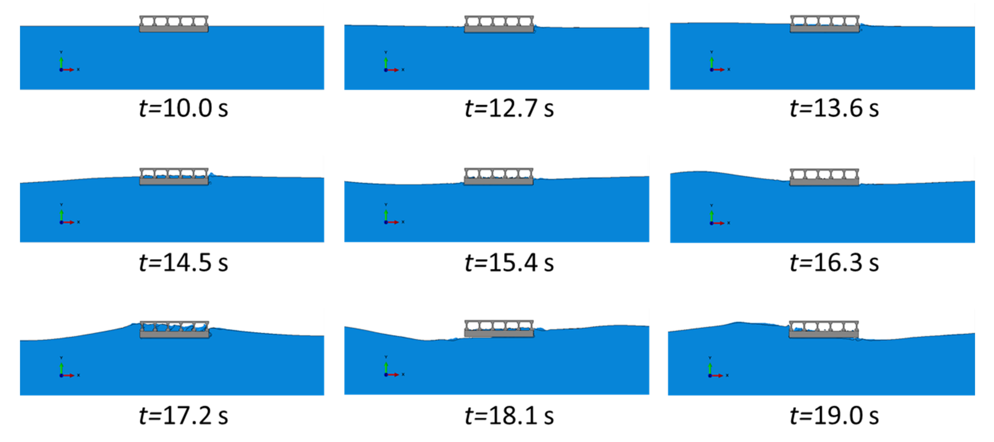
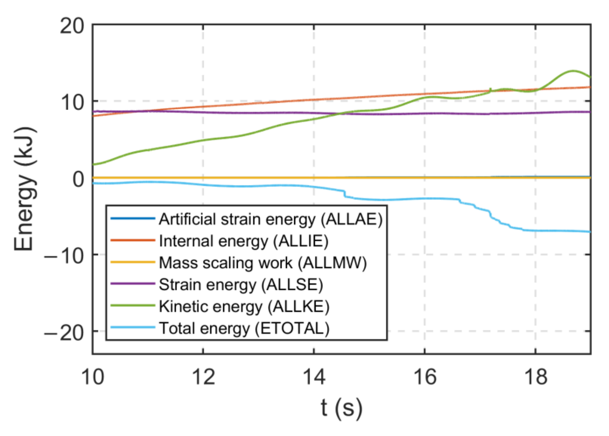
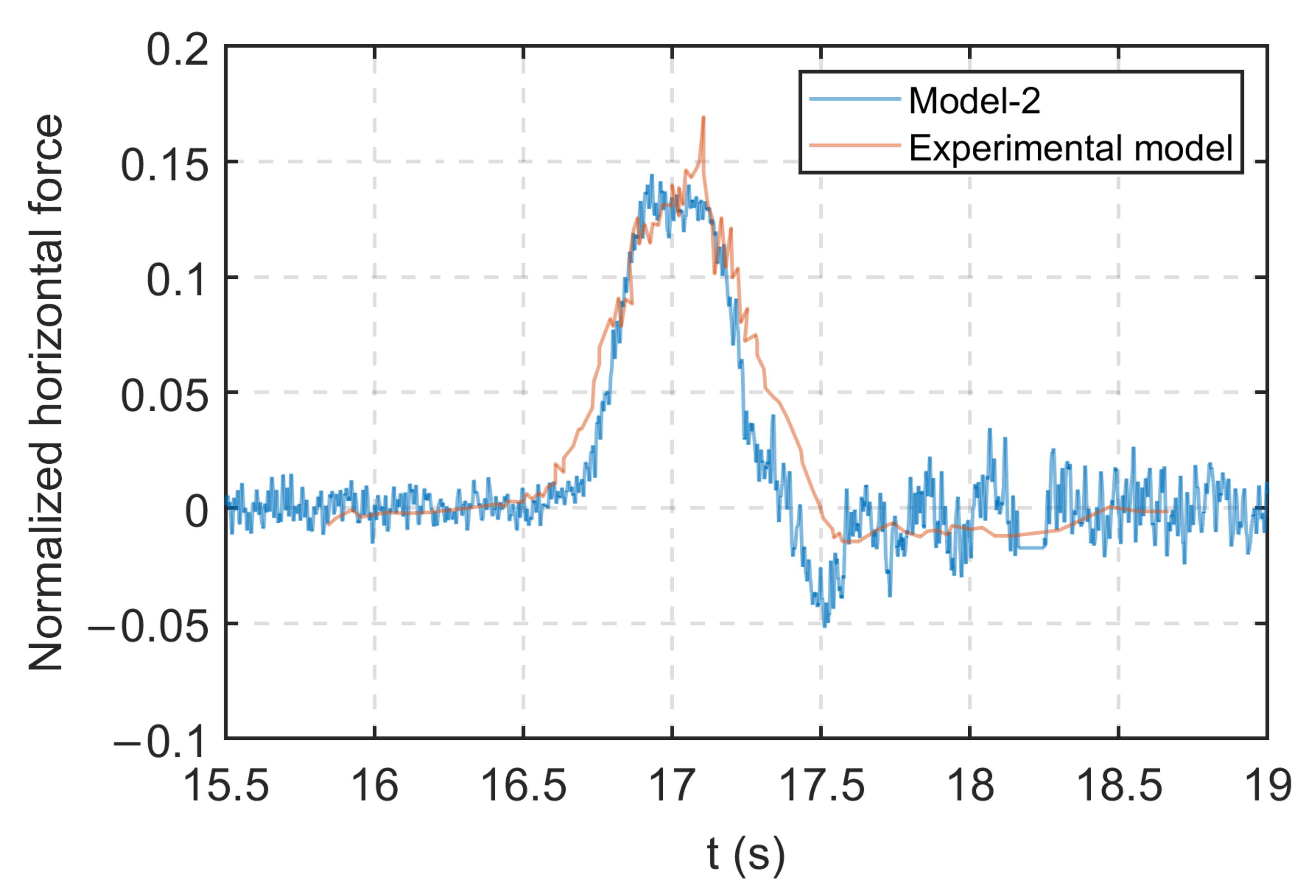
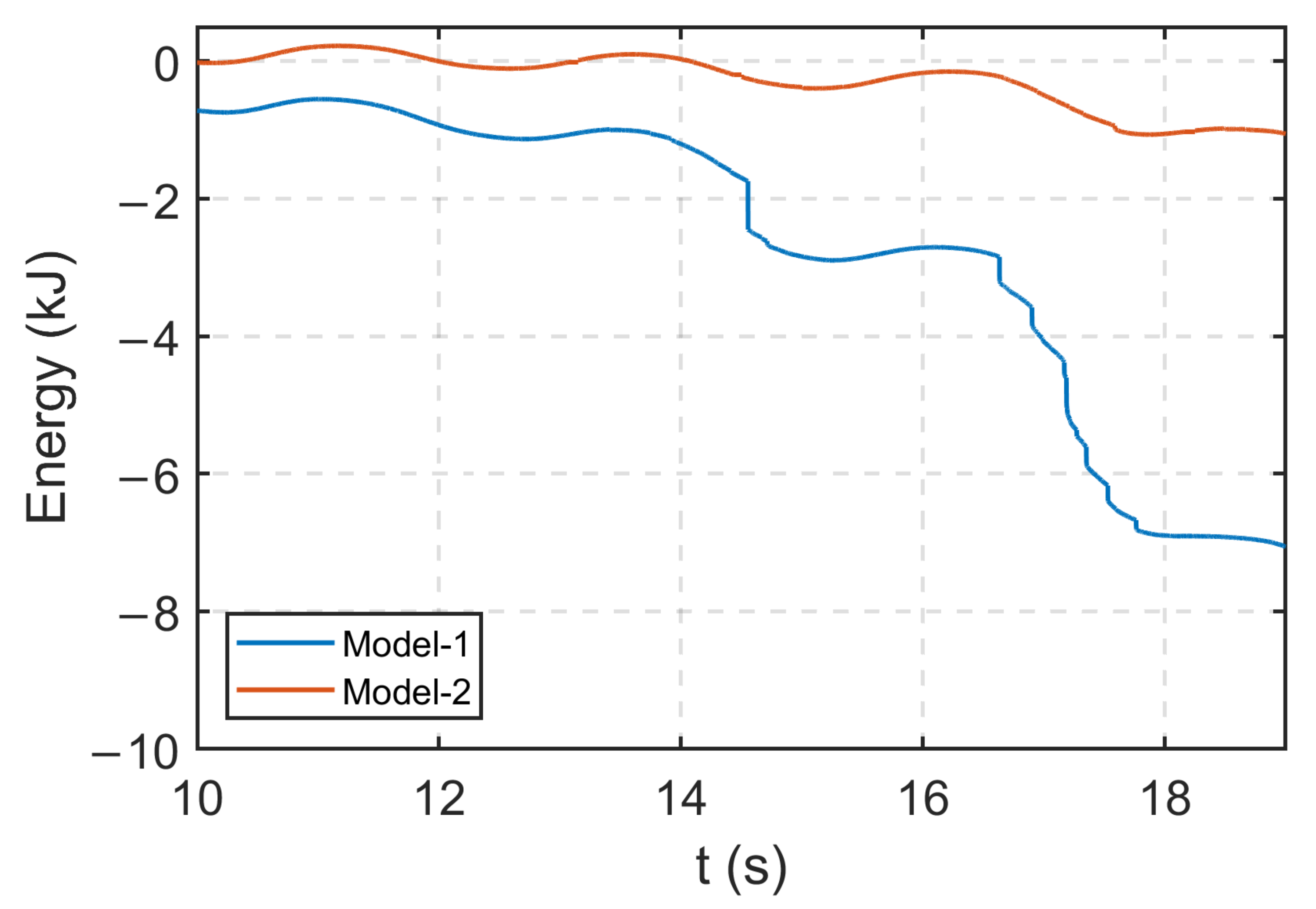
• The energy balance shown in Figure 13 indicates that the numerical artifacts were likely the result of Eulerian–Lagrangian surface interactions when waves impacted the bridge superstructure. It was observed that numerical artifacts in the unfiltered signals were significantly reduced after optimizing the modeling parameters defining the contact interaction between the Eulerian and Lagrangian elements.
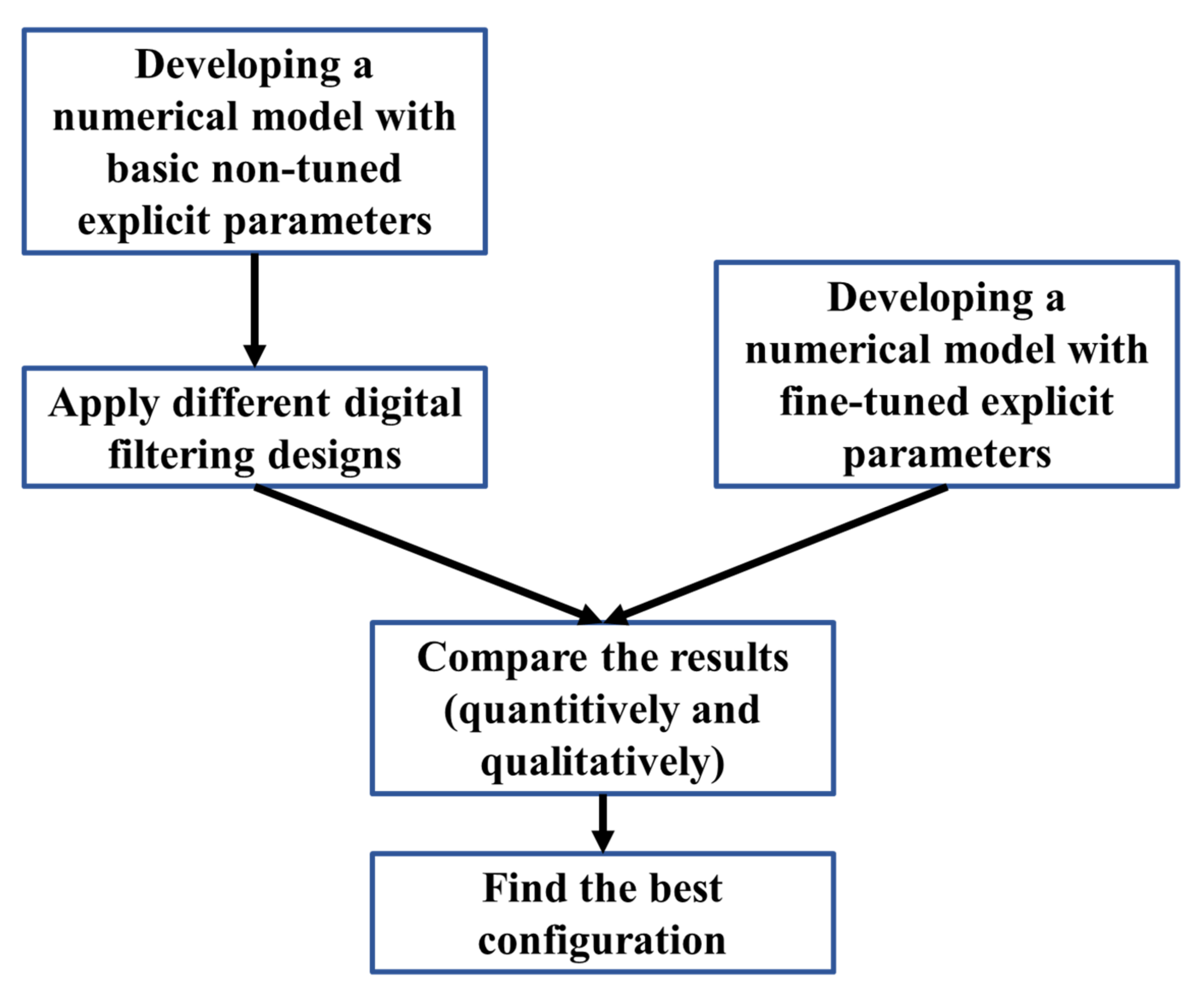
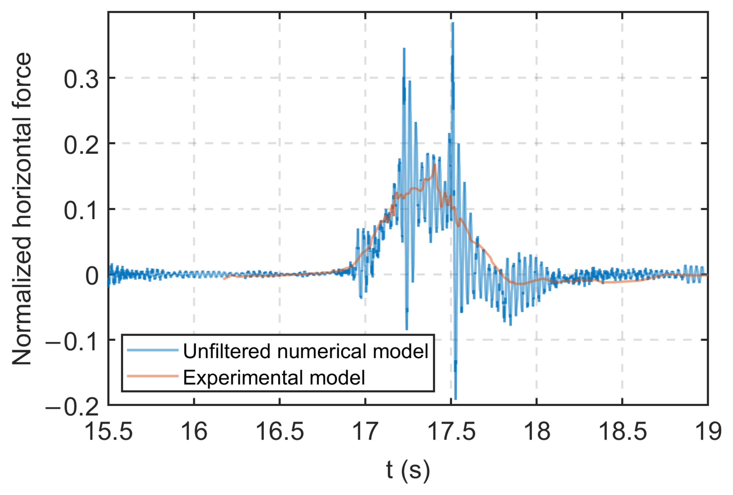
• A poor choice of modeling parameters in CEL models was shown to lead to unwanted force signal oscillations and an increase in total energy. This deficiency can be addressed by either optimizing the modeling parameters of the FE model or filtering the force signal.
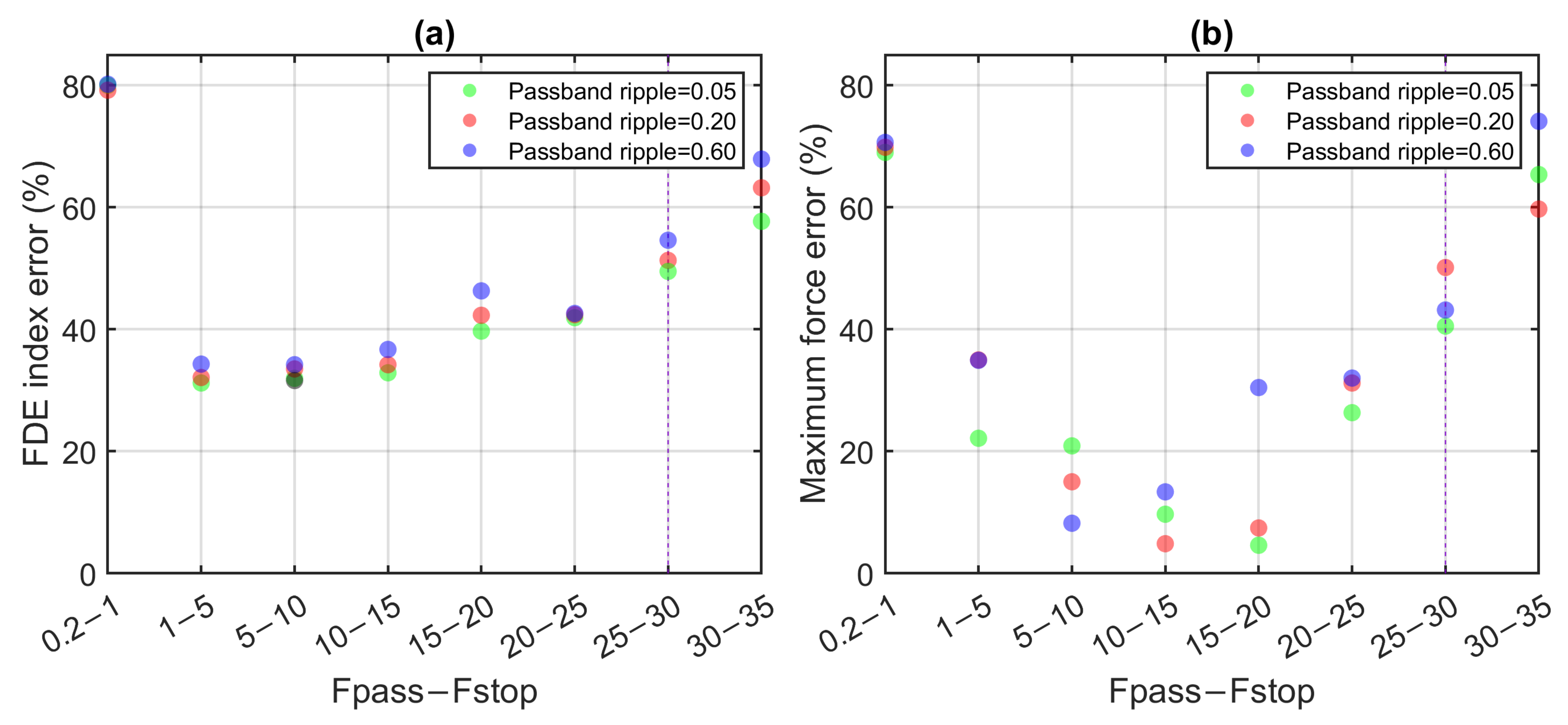
• Although a clear relationship was observed between the FDE index of filtered force signals and passband ripple magnitude, no discernible trend was observed in the relationship between maximum force error and passband ripple magnitude.
• Filter configurations that provided the lowest FDE index error did not provide the lowest maximum force error.
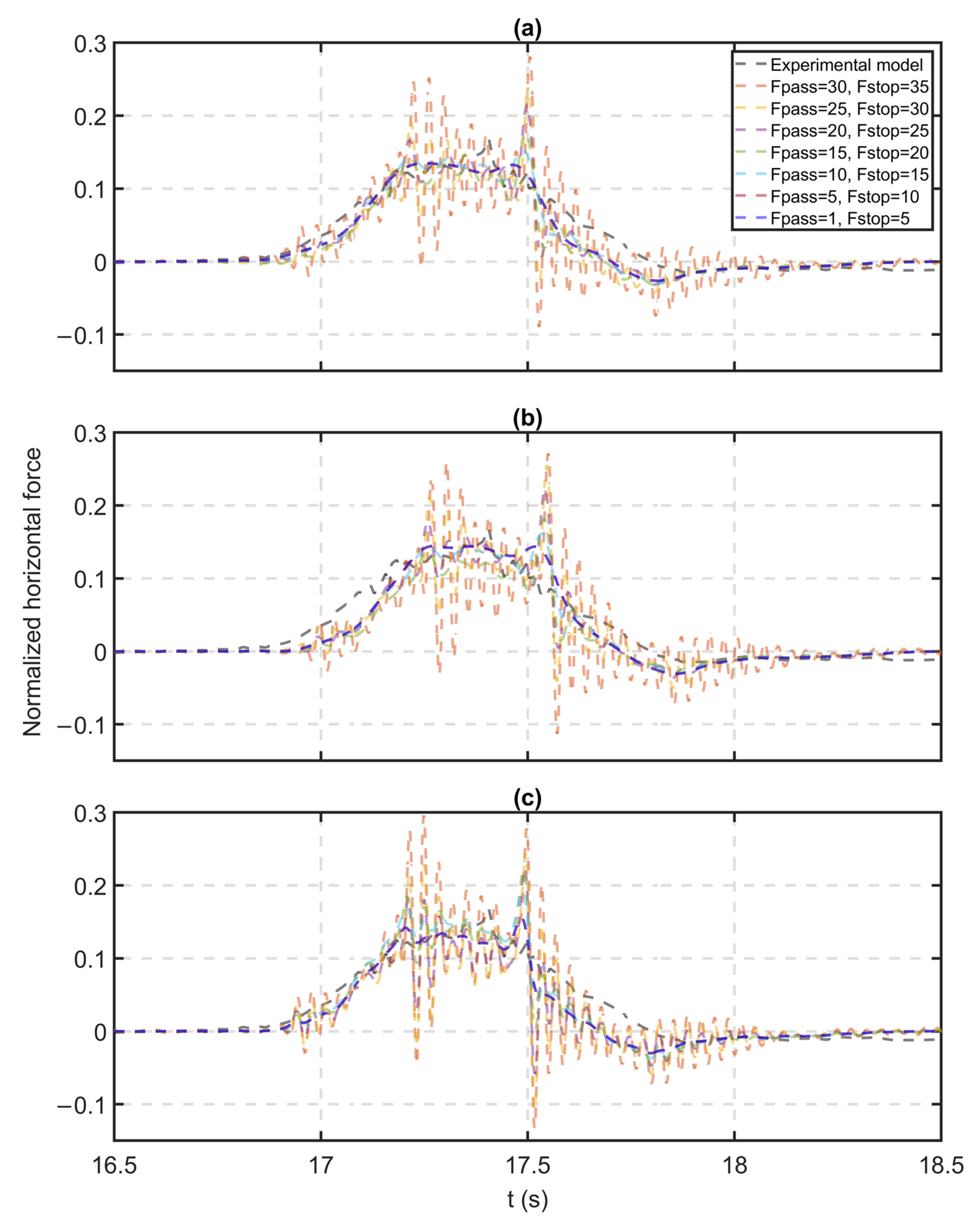
• Applying a filter to the force signal from model 1 with a passband frequency equal to the fundamental frequency of the superstructure produced a FDE index similar to that of the unfiltered signal calculated with optimized model 2, although the maximum force error of the model 1-filtered signal was significantly higher than the maximum error of the unfiltered signal from model 2.
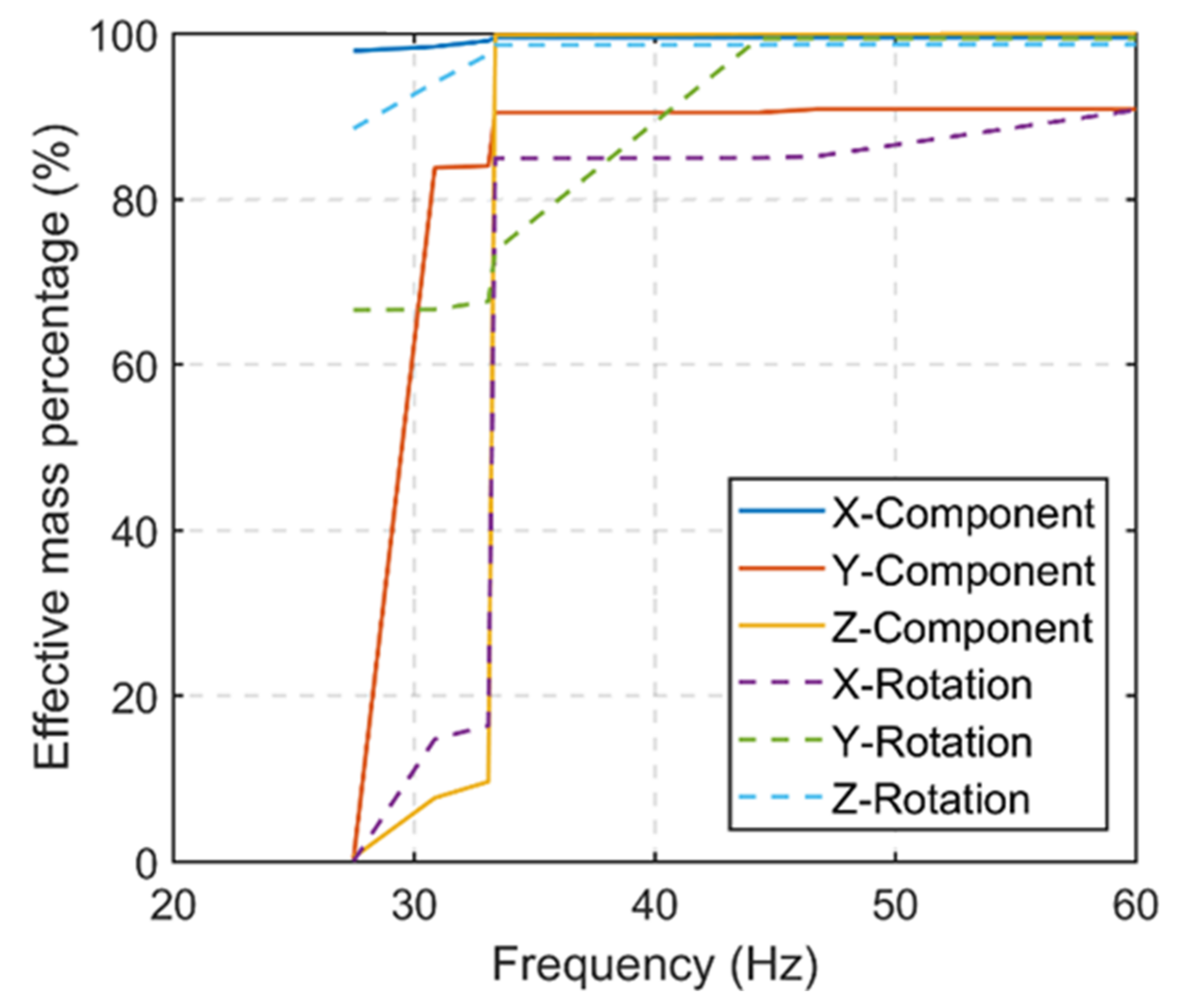
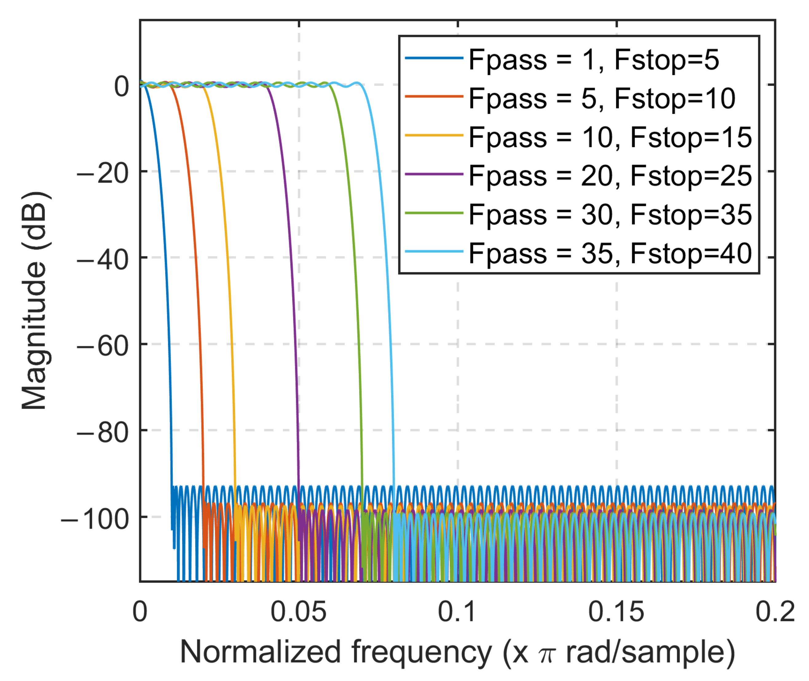
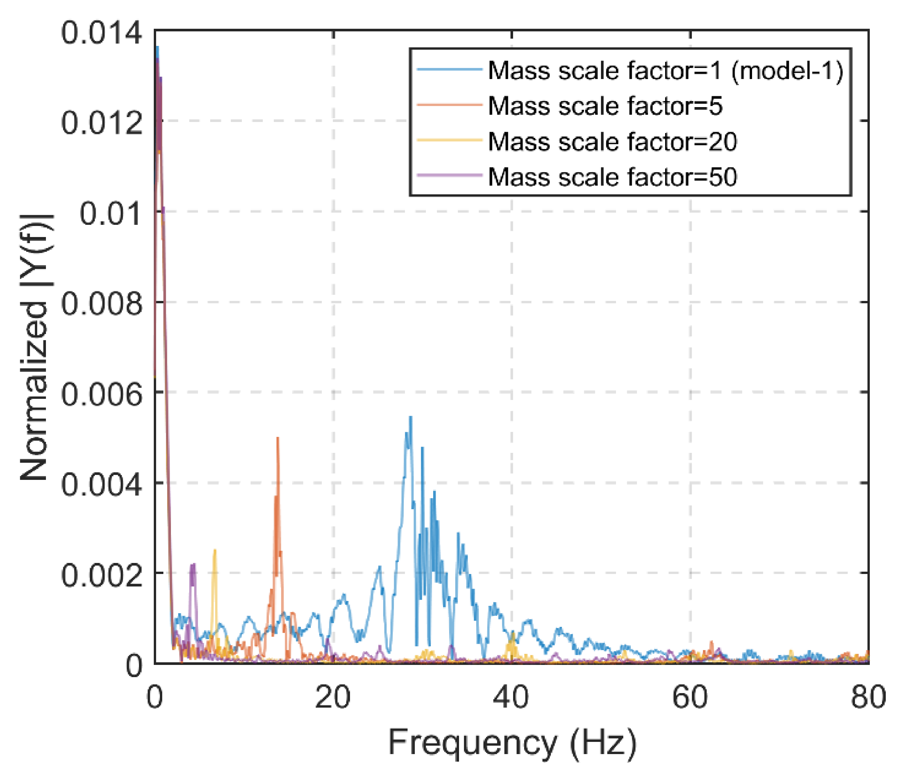
• Filter configurations with stopband and passband frequencies (1 to 20 Hz) lower than the fundamental frequency of the superstructure, approximately 27 Hz based on the FFT of the calculated force signal (Figure 14), produced the lowest FDE index and maximum force errors.
• The optimized parameters used in model 2 (Table 4) were shown to be effective in reducing force signal artifacts and are recommended for future studies analyzing wave–superstructure interactions.

References

- Nickas, W.N.; Renna, R.; Sheppard, N.; Mertz, D.R. Hurricane-Based Wave Attacks; Florida Department of Transportation: Tallahassee, FL, USA, 2005.
- Huang, B.; Zhu, B.; Cui, S.; Duan, L.; Zhang, J. Experimental and Numerical Modelling of Wave Forces on Coastal Bridge Superstructures with Box Girders, Part I: Regular Waves. Ocean Eng. 2018, 149, 53–77. [Google Scholar] [CrossRef]
- Zhu, D.; Dong, Y. Experimental and 3D Numerical Investigation of Solitary Wave Forces on Coastal Bridges. Ocean Eng. 2020, 209, 107499. [Google Scholar] [CrossRef]
- Marin, J.; Sheppard, D.M. Storm Surge and Wave Loading on Bridge Superstructures. In Proceedings of the Structures Congress 2009: Don’t Mess with Structural Engineers: Expanding Our Role, Austin, TX, USA, 30 April–2 May 2009; pp. 1–10. [Google Scholar]
- Kerenyi, K.; Sofu, T.; Guo, J. Hydrodynamic Forces on Inundated Bridge Decks; U.S. Department of Transportation: Mclean, VA, USA, 2009.
- Lau, T.L.; Ohmachi, T.; Inoue, S.; Lukkunaprasit, P. Experimental and Numerical Modeling of Tsunami Force on Bridge Decks; InTech: Rijeka, Croatia, 2011. [Google Scholar]
- Bozorgnia, M. Computational Fluid Dynamic Analysis of Highway Bridge Superstructures Exposed to Hurricane Waves; University of Southern California: Los Angeles, CA, USA, 2012; ISBN 1267892595. [Google Scholar]
- Bradner, C.; Schumacher, T.; Cox, D.; Higgins, C. Experimental Setup for a Large-Scale Bridge Superstructure Model Subjected to Waves. J. Waterw. Port Coast. Ocean. Eng. 2011, 137, 3–11. [Google Scholar] [CrossRef]
- Yim, S.C.; Azadbakht, M. Tsunami Forces on Selected California Coastal Bridges; California Department of Transportation: Sacramento, CA, USA, 2013.
- Lee, K.; Jeong, S. Large Deformation FE Analysis of a Debris Flow with Entrainment of the Soil Layer. Comput. Geotech. 2018, 96, 258–268. [Google Scholar] [CrossRef]
- Cao, Y.; Liu, C.; Tian, H.; Sun, Y.; Zhang, S. Mechanical Behaviors of Pipeline Inspection Gauge (Pig) in Launching Process Based on Coupled Eulerian-Lagrangian (CEL) Method. Int. J. Press. Vessel. Pip. 2022, 197, 104622. [Google Scholar] [CrossRef]
- Jeong, S.; Lee, K. Analysis of the Impact Force of Debris Flows on a Check Dam by Using a Coupled Eulerian-Lagrangian (CEL) Method. Comput. Geotech. 2019, 116, 103214. [Google Scholar] [CrossRef]
- Liu, C.; Huang, Z. A Mixed Eulerian-Lagrangian Simulation of Nonlinear Wave Interaction with a Fluid-Filled Membrane Breakwater. Ocean Eng. 2019, 178, 423–434. [Google Scholar] [CrossRef]
- Liu, S.; Tang, X.; Li, J. A Decoupled Arbitrary Lagrangian-Eulerian Method for Large Deformation Analysis of Saturated Sand. Soils Found. 2022, 62, 101110. [Google Scholar] [CrossRef]
- Gargari, S.F.; Kolahdoozan, M.; Afshar, M.H.; Dabiri, S. An Eulerian–Lagrangian Mixed Discrete Least Squares Meshfree Method for Incompressible Multiphase Flow Problems. Appl. Math. Model. 2019, 76, 193–224. [Google Scholar] [CrossRef]
- Majlesi, A.; Amori, D.; Montoya, A.; Du, A.; Matamoros, A.; Shahriar, A.; Nasouri, R. Eulerian-Lagrangian Simulation of Wave Impact on Coastal Bridges. In Bridge Safety, Maintenance, Management, Life-Cycle, Resilience and Sustainability; CRC Press: Boca Raton, FL, USA, 2022; pp. 117–125. ISBN 1003322646. [Google Scholar]
- Nasouri, R.; Shahriar, A.; Majlesi, A.; Matamoros, A.; Montoya, A.; Testik, F.Y. Hydrodynamic Demands on Coastal Bridges Due to Wave Impact. In Bridge Maintenance, Safety, Management, Life-Cycle Sustainability and Innovations; CRC Press: Boca Raton, FL, USA, 2021; pp. 1241–1248. ISBN 0429279116. [Google Scholar]
- Xiang, T.; Istrati, D. Assessment of Extreme Wave Impact on Coastal Decks with Different Geometries via the Arbitrary Lagrangian-Eulerian Method. J. Mar. Sci. Eng. 2021, 9, 1342. [Google Scholar] [CrossRef]
- Do, T.Q.; van de Lindt, J.W.; Cox, D.T. Performance-Based Design Methodology for Inundated Elevated Coastal Structures Subjected to Wave Load. Eng. Struct. 2016, 117, 250–262. [Google Scholar] [CrossRef]
- Montoya, A.; Matamoros, A.; Testik, F.; Nasouri, R.; Shahriar, A.; Majlesi, A. Structural Vulnerability of Coastal Bridges under Extreme Hurricane Conditions; Transportation Consortium of South-Central States: Baton Rouge, LA, USA, 2019.
- Majlesi, A.; Nasouri, R.; Shahriar, A.; Montoya, A.; Matamoros, A. Structural Vulnerability of Coastal Bridges under a Variety of Hydrodynamic Conditions. In Tran-SET 2020; American Society of Civil Engineers: Reston, VA, USA, 2021; pp. 120–125. [Google Scholar]
- Xiang, T.; Istrati, D.; Yim, S.C.; Buckle, I.G.; Lomonaco, P. Tsunami Loads on a Representative Coastal Bridge Deck: Experimental Study and Validation of Design Equations. J. Waterw. Port Coast. Ocean Eng. 2020, 146, 4020022. [Google Scholar] [CrossRef]
- Fang, Q.; Liu, J.; Hong, R.; Guo, A.; Li, H. Experimental Investigation of Focused Wave Action on Coastal Bridges with Box Girder. Coast. Eng. 2021, 165, 103857. [Google Scholar] [CrossRef]
- Istrati, D.; Buckle, I.; Lomonaco, P.; Yim, S. Deciphering the Tsunami Wave Impact and Associated Connection Forces in Open-Girder Coastal Bridges. J. Mar. Sci. Eng. 2018, 6, 148. [Google Scholar] [CrossRef]
- Xu, G.; Chen, Q.; Zhu, L.; Chakrabarti, A. Characteristics of the Wave Loads on Coastal Low-Lying Twin-Deck Bridges. J. Perform. Constr. Facil. 2018, 32, 4017132. [Google Scholar] [CrossRef]
- Yim, S.C.; Olsen, M.J.; Cheung, K.F.; Azadbakht, M. Tsunami Modeling, Fluid Load Simulation, and Validation Using Geospatial Field Data. J. Struct. Eng. 2014, 140, A4014012. [Google Scholar] [CrossRef]
- Azadbakht, M.; Yim, S.C. Bridge Superstructure Design for Tsunamis: A State-of-the-Art Methodology for Tsunami Modeling, Load Simulation, and Structural Response Assessment. In Proceedings of the Structures Congress 2015, Oregon, Portland, 23–25 April 2015; pp. 345–354. [Google Scholar]
- Azadbakht, M.; Yim, S.C. Effect of Trapped Air on Wave Forces on Coastal Bridge Superstructures. J. Ocean Eng. Mar. Energy 2016, 2, 139–158. [Google Scholar] [CrossRef]
- Azadbakht, M.; Yim, S.C. Simulation and Estimation of Tsunami Loads on Bridge Superstructures. J. Waterw. Port Coast. Ocean Eng. 2015, 141, 4014031. [Google Scholar] [CrossRef]
- Majlesi, A.; Nasouri, R.; Shahriar, A.; Amori, D.; Montoya, A.; Du, A.; Matamoros, A. Explicit Finite Element Analysis of Coastal Bridges under Extreme Hurricane Waves. In Tran-SET 2021; American Society of Civil Engineers: Reston, VA, USA, 2021; pp. 324–331. [Google Scholar]
- Ataei, N.; Padgett, J.E. Influential Fluid–Structure Interaction Modelling Parameters on the Response of Bridges Vulnerable to Coastal Storms. Struct. Infrastruct. Eng. 2015, 11, 321–333. [Google Scholar] [CrossRef]
- Majlesi, A.; Asadi-Ghoozhdi, H.; Bamshad, O.; Attarnejad, R.; Masoodi, A.R.; Ghassemieh, M. On the Seismic Evaluation of Steel Frames Laterally Braced with Perforated Steel Plate Shear Walls Considering Semi-Rigid Connections. Buildings 2022, 12, 1427. [Google Scholar] [CrossRef]
- Schumacher, T.; Hameed, A.W.; Higgins, C.; Erickson, B. Characterization of Hydrodynamic Properties from Free Vibration Tests of a Large-Scale Bridge Model. J. Fluids Struct. 2021, 106, 103368. [Google Scholar] [CrossRef]
- Douglass, S.; Chen, Q.; Olsen, J. Wave Forces on Bridge Decks; Final Report; U.S. Department of Transportation and Federal Highway Administration Office of Bridge Technology: Washington, DC, USA, 2006.
- Cuomo, G.; Tirindelli, M.; Allsop, W. Wave-in-Deck Loads on Exposed Jetties. Coast. Eng. 2007, 54, 657–679. [Google Scholar] [CrossRef]
- Bradner, C.; Schumacher, T.; Cox, D.; Higgins, C. Large–Scale Laboratory Observations of Wave Forces on a Highway Bridge Superstructure; Transportation Research and Education Center: Portland, OR, USA, 2011. [Google Scholar]
- Simulia, A.V. 6.13 Documentation; Dassault Systemes: Velizy-Villacoublay, France, 2013. [Google Scholar]
- Shahriar, A.; Majlesi, A.; Nasouri, R.; Montoya, A.; Matamoros, A.; Testik, F. Generation of Periodic Wave Using Lagrange-Plus Remap Finite Element Method for Evaluating the Vulnerability of Coastal Bridges to Extreme Weather Events. In Tran-SET 2020; American Society of Civil Engineers: Reston, VA, USA, 2021; pp. 133–140. [Google Scholar]
- Dean, R.G. Water Wave Mechanics for Engineers and Scientists. Adv. Ser. Ocean Eng. 1984, 2, 353. [Google Scholar]
- Lamb, H. Hydrodynamics; Dover Publications: New York, NY, USA, 1945. [Google Scholar]
- Madsen, O.S. On the Generation of Long Waves. J. Geophys. Res. 1971, 76, 8672–8683. [Google Scholar] [CrossRef]
- Qiu, G.; Henke, S.; Grabe, J. Application of a Coupled Eulerian–Lagrangian Approach on Geomechanical Problems Involving Large Deformations. Comput. Geotech. 2011, 38, 30–39. [Google Scholar] [CrossRef]
- Benson, D.J. Computational Methods in Lagrangian and Eulerian Hydrocodes. Comput. Methods Appl. Mech. Eng. 1992, 99, 235–394. [Google Scholar] [CrossRef]
- Benson, D.J.; Okazawa, S. Contact in a Multi-Material Eulerian Finite Element Formulation. Comput. Methods Appl. Mech. Eng. 2004, 193, 4277–4298. [Google Scholar] [CrossRef]
- Abaqus, V. 6.14 Documentation; Dassault Systemes Simulia Corporation: Providence, RI, USA, 2014; p. 651. [Google Scholar]
- Olovsson, L.; Simonsson, K.; Unosson, M. Selective Mass Scaling for Explicit Finite Element Analyses. Int. J. Numer. Methods Eng. 2005, 63, 1436–1445. [Google Scholar] [CrossRef]
- Dragovich, J.J.; Lepage, A. FDE Index for Goodness-of-fit between Measured and Calculated Response Signals. Earthq. Eng. Struct. Dyn. 2009, 38, 1751–1758. [Google Scholar] [CrossRef]