


Offshore Measurements and Numerical Validation of the Mooring Forces on a 1:5 Scale Buoy

 ,
,  ,
,  , and
, and
Abstract
1. Introduction
2. Method
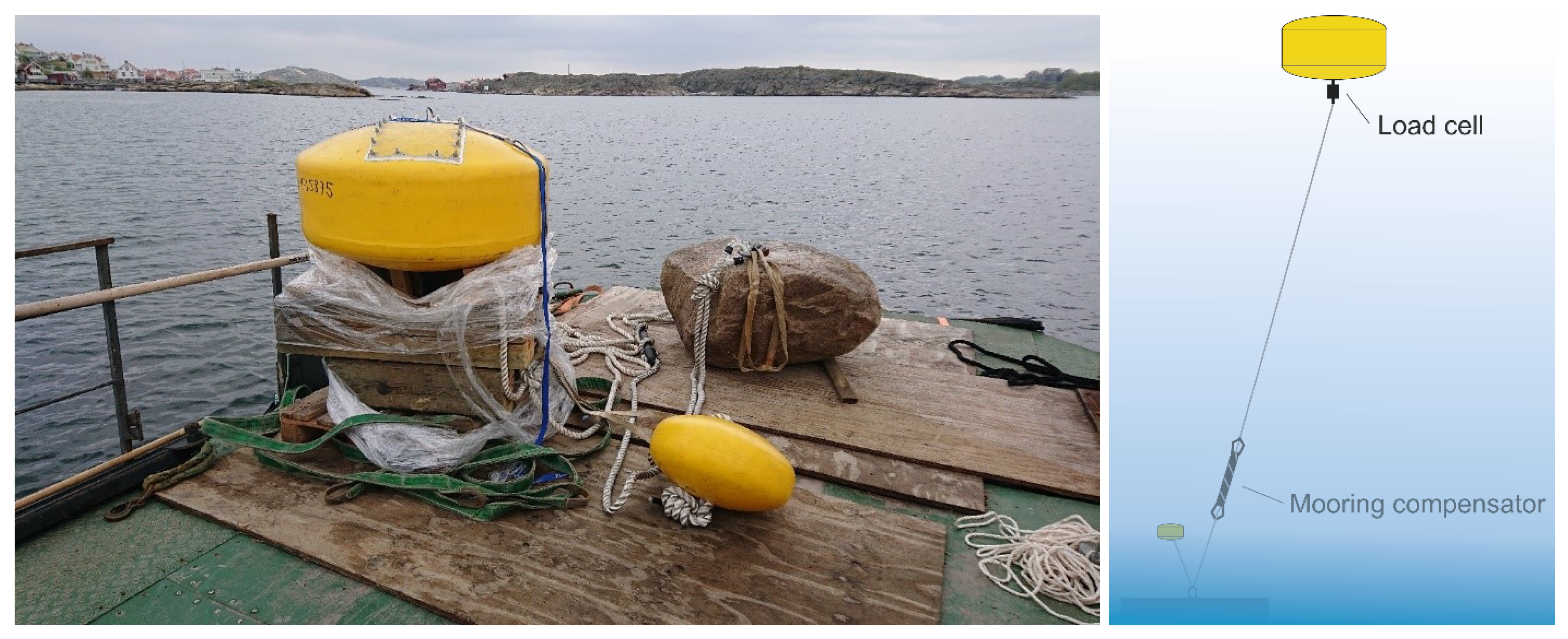
2.1. Experiment
2.2. Test Site
2.3. Numerical Modelling
2.3.1. Linear Model
2.3.2. CFD Model
2.4. Extreme Value Analysis
3. Results
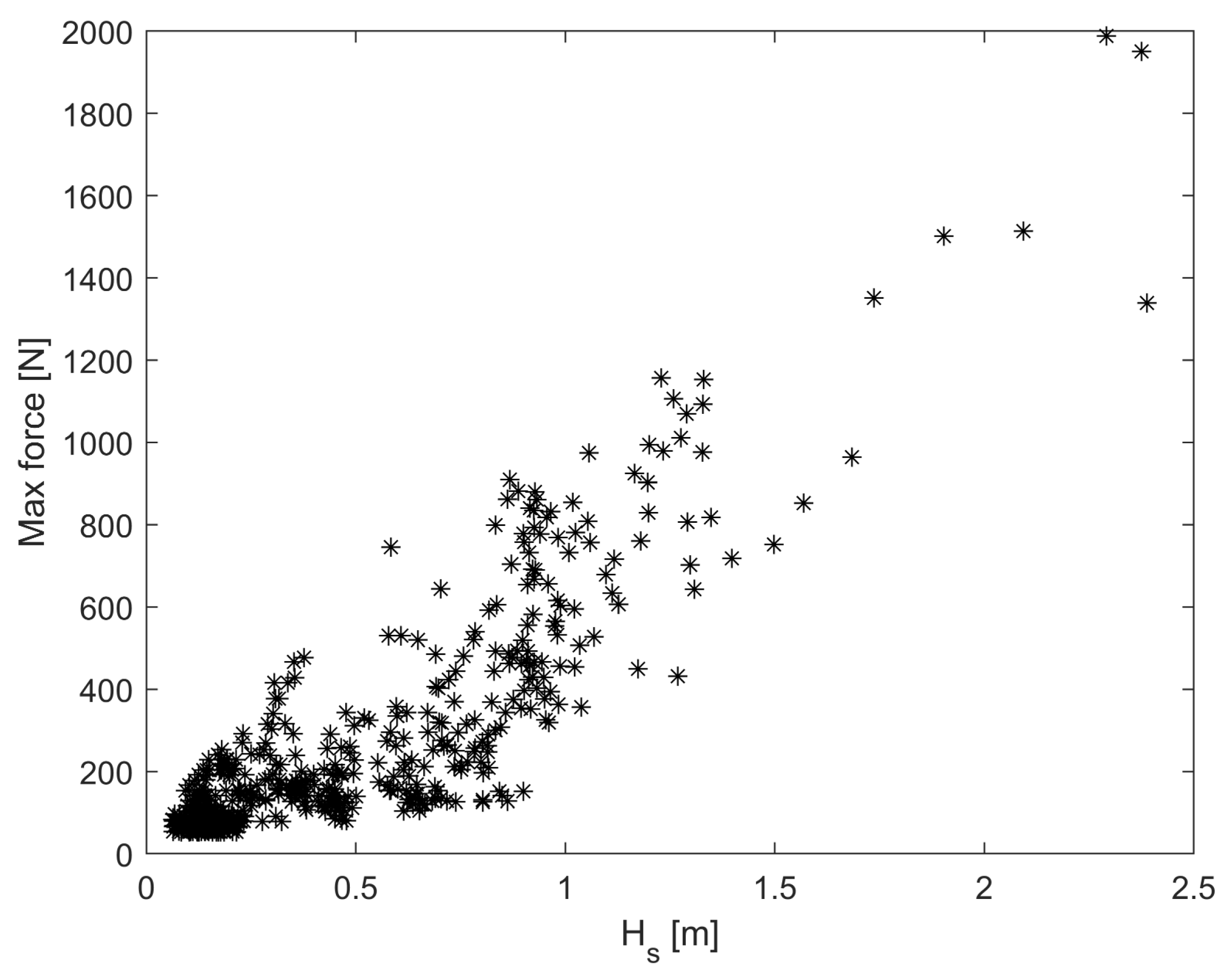
3.1. Offshore Experiments
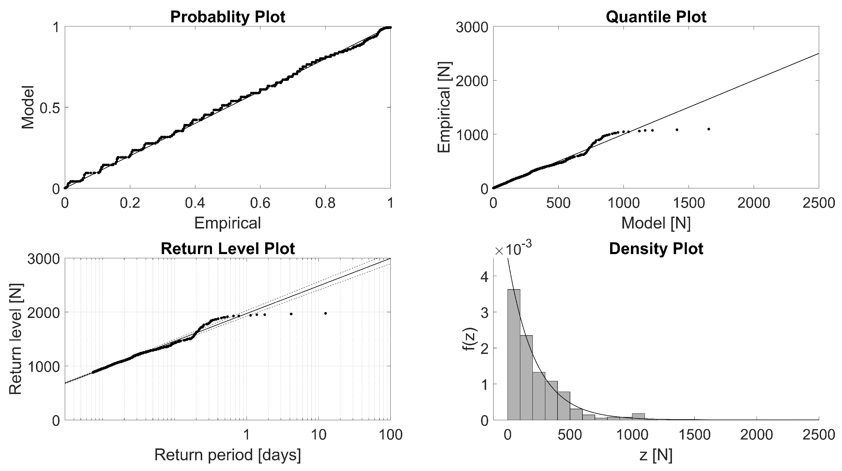
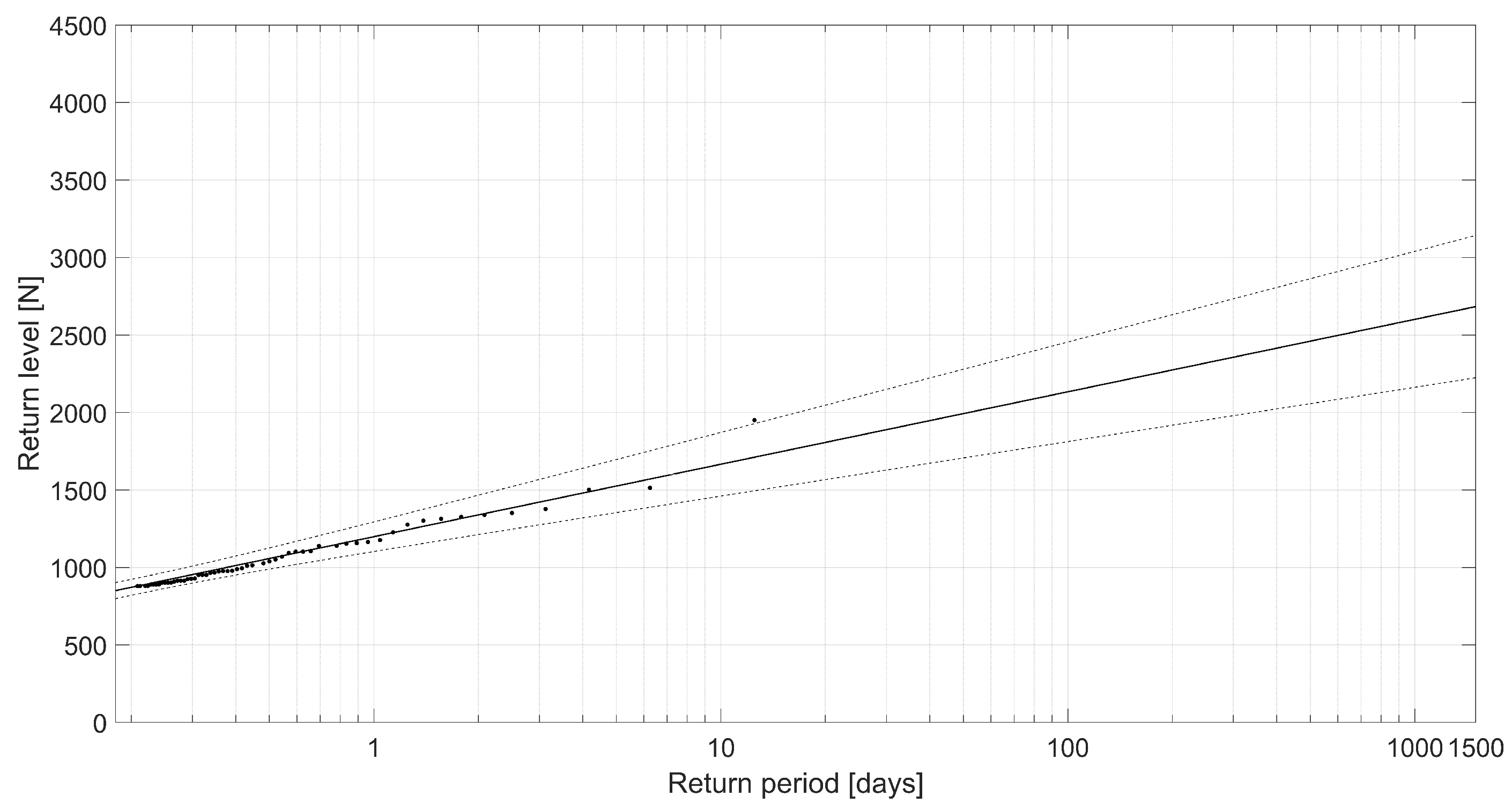
3.2. Extreme Loads and Loads over Threshold Analysis
3.3. Comparison to Numerical Simulations
4. Discussion
5. Conclusions
- (a)
- Forces up to 2 kN were observed;
- (b)
- Even for waves of similar significant wave height, a large variance in maximum force was measured.
Author Contributions
Funding
Acknowledgments
Conflicts of Interest
References
- Czech, B.; Bauer, P. Wave energy converter concepts: Design challenges and classification. IEEE Ind. Electron. Mag. 2012, 6, 4–16. [Google Scholar] [CrossRef]
- Ransley, E.J. Survivability of Wave Energy Converter and Mooring Coupled System Using CFD; Plymouth University: Plymouth, UK, 2015. [Google Scholar]
- Jonathan, P.; Ewans, K. Statistical modelling of extreme ocean environments for marine design: A review. Ocean Eng. 2013, 62, 91–109. [Google Scholar] [CrossRef]
- Eriksson, M.; Waters, R.; Svensson, O.; Isberg, J.; Leijon, M. Wave power absorption: Experiments in open sea and simulation. J. Appl. Phys. 2007, 102, 084910. [Google Scholar] [CrossRef]
- Marquis, L.; Kramer, M.; Frigaard, P. First power production figures from the Wave Star Roshage wave energy converter. In Proceedings of the 3rd International Conference on Ocean Energy (ICOE-2010), Bilbao, Spain, 6 October 2010; Volume 68, pp. 1–5. [Google Scholar]
- Yemm, R.; Pizer, D.; Retzler, C.; Henderson, R. Pelamis: Experience from concept to connection. Philos. Trans. R. Soc. A Math. Phys. Eng. Sci. 2012, 370, 365–380. [Google Scholar] [CrossRef] [PubMed]
- Ibarra-Berastegi, G.; Sáenz, J.; Ulazia, A.; Serras, P.; Esnaola, G.; Garcia-Soto, C. Electricity production, capacity factor, and plant efficiency index at the Mutriku wave farm (2014–2016). Ocean Eng. 2018, 147, 20–29. [Google Scholar] [CrossRef]
- O’Sullivan, D.; Griffiths, J.; Egan, M.G.; Lewis, A.W. Development of an electrical power take off system for a sea-test scaled offshore wave energy device. Renew. Energy 2011, 36, 1236–1244. [Google Scholar] [CrossRef]
- Ransley, E.; Hann, M.; Greaves, D.; Raby, A.; Simmonds, D. Numerical and physical modelling of extreme wave impacts on a fixed truncated circular cylinder. In Proceedings of the 10th European Wave and Tidal Energy Conference (EWTEC), Aalborg, Denmark, 2–5 September 2013. [Google Scholar]
- Viuff, T.H.; Andersen, M.T.; Kramer, M.; Jakobsen, M.M. Excitation forces on point absorbers exposed to high order non-linear waves. In Proceedings of the European Wave and Tidal Energy Conference. Technical Committee of the European Wave and Tidal Energy Conference, Aalborg, Denmark, 2–5 September 2013. [Google Scholar]
- Svensson, O.; Leijon, M. Peak force measurements on a cylindrical buoy with limited elastic mooring. IEEE J. Ocean. Eng. 2013, 39, 398–403. [Google Scholar] [CrossRef]
- Weller, S.D.; Thies, P.R.; Gordelier, T.; Johanning, L. Reducing reliability uncertainties for marine renewable energy. J. Mar. Sci. Eng. 2015, 3, 1349–1361. [Google Scholar] [CrossRef]
- Kofoed, J.P.; Frigaard, P.; Friis-Madsen, E.; Sørensen, H.C. Prototype testing of the wave energy converter wave dragon. Renew. Energy 2006, 31, 181–189. [Google Scholar] [CrossRef]
- Hennessey, C.; Pearson, N.; Plaut, R.H. Experimental snap loading of synthetic ropes. Shock Vib. 2005, 12, 163–175. [Google Scholar] [CrossRef]
- Göteman, M.; Engström, J.; Eriksson, M.; Hann, M.; Ransley, E.; Greaves, D.; Leijon, M. Wave loads on a point-absorbing wave energy device in extreme waves. In Proceedings of the The Twenty-Fifth International Ocean and Polar Engineering Conference, Kona, HI, USA, 21–26 June 2015; OnePetro: Kona, HI, USA, 2015. [Google Scholar]
- Coe, R.G.; Rosenberg, B.J.; Quon, E.W.; Chartrand, C.C.; Yu, Y.H.; van Rij, J.; Mundon, T.R. CFD design-load analysis of a two-body wave energy converter. J. Ocean. Eng. Mar. Energy 2019, 5, 99–117. [Google Scholar] [CrossRef]
- Hu, Z.Z.; Greaves, D.; Raby, A. Numerical wave tank study of extreme waves and wave-structure interaction using OpenFOAM®. Ocean Eng. 2016, 126, 329–342. [Google Scholar] [CrossRef]
- Katsidoniotaki, E.; Göteman, M. Numerical modeling of extreme wave interaction with point-absorber using OpenFOAM. Ocean Eng. 2022, 245, 110268. [Google Scholar] [CrossRef]
- Tagliafierro, B.; Martínez-Estévez, I.; Domínguez, J.M.; Crespo, A.J.; Göteman, M.; Engström, J.; Gómez-Gesteira, M. A numerical study of a taut-moored point-absorber wave energy converter with a linear power take-off system under extreme wave conditions. Appl. Energy 2022, 311, 118629. [Google Scholar] [CrossRef]
- Toro, E.F. Shock-Capturing Methods for Free-Surface Shallow Flows; Wiley-Blackwell: Hoboken, NJ, USA, 2001. [Google Scholar]
- Waters, R.; Engström, J.; Isberg, J.; Leijon, M. Wave climate off the Swedish west coast. Renew. Energy 2009, 34, 1600–1606. [Google Scholar] [CrossRef]
- Leijon, M.; Boström, C.; Danielsson, O.; Gustafsson, S.; Haikonen, K.; Langhamer, O.; Strömstedt, E.; Stålberg, M.; Sundberg, J.; Svensson, O.; et al. Wave energy from the North Sea: Experiences from the Lysekil research site. Surv. Geophys. 2008, 29, 221–240. [Google Scholar] [CrossRef]
- Weller, H.G. Derivation, Modelling and Solution of the Conditionally Averaged Two-Phase Flow Equations; Technical Report TR/HGW, 2, 9; Nabla Ltd.: Boston, MA, USA, 2002. [Google Scholar]
- Katsidoniotaki, E.; Göteman, M. Comparison of dynamic mesh methods in OpenFOAM for a WEC in extreme waves. In Developments in Renewable Energies Offshore; CRC Press: Boca Raton, FL, USA, 2020; pp. 214–222. [Google Scholar]
- Schmitt, P.; Elsaesser, B. On the use of OpenFOAM to model oscillating wave surge converters. Ocean Eng. 2015, 108, 98–104. [Google Scholar] [CrossRef]
- Windt, C.; Davidson, J.; Ringwood, J.V. Investigation of turbulence modeling for point-absorber-type wave energy converters. Energies 2020, 14, 26. [Google Scholar] [CrossRef]
- Katsidoniotaki, E.; Nilsson, E.; Rutgersson, A.; Engström, J.; Göteman, M. Response of point-absorbing wave energy conversion system in 50-years return period extreme focused waves. J. Mar. Sci. Eng. 2021, 9, 345. [Google Scholar] [CrossRef]
- International Towing Tank Conference. Practical Guidelines for Numerical Modelling of Wave Energy Converter. 2021. Available online: https://www.ittc.info/media/9737/75-02-07-0318.pdf (accessed on 11 January 2023).
- Schlichting, H.; Gersten, K. Boundary-Layer Theory; Springer Science & Business Media: Berlin/Heidelberg, Germany, 2003. [Google Scholar]
- Det Norske Veritas, A. Environmental Conditions and Environmental Loads; DNV-RP-C205; Det Norske Veritas: Oslo, Norway, 2010. [Google Scholar]
- World Meteorological Organization. Guide to Wave Analysis and Forecasting; Secretariat of the World Meteorological Organization: Geneva, Switzerland, 1998. [Google Scholar]
- Coles, S.; Bawa, J.; Trenner, L.; Dorazio, P. An Introduction to Statistical Modeling of Extreme Values; Springer: Berlin/Heidelberg, Germany, 2001; Volume 208. [Google Scholar]
- Palm, J.; Eskilsson, C.; Paredes, G.M.; Bergdahl, L. CFD simulation of a moored floating wave energy converter. In Proceedings of the 10th European Wave and Tidal Energy Conference, Aalborg, Denmark, 1–5 September 2013; Volume 25. [Google Scholar]


| Parameter | Value | Unit | Parameter | Value | Unit |
|---|---|---|---|---|---|
| Buoy diameter | 1 | m | Buoy volume | 0.35 | m3 |
| Buoy height | 0.55 | m | Water depth | 25 | m |
| Buoy draft | 0.15 | m | Spring constant | 5000 | N/m |
| Buoy mass | 81 | kg | Mass of foundation | 1000 | kg |
| Sea State | [m] | [s] | H [m] | T [s] | KC |
|---|---|---|---|---|---|
| # 1 | 0.90 | 5.45 | 1.71 | 5.45 | 5.37 |
| # 2 | 1.02 | 7.63 | 1.95 | 7.63 | 6.12 |
| # 3 | 1.40 | 5.74 | 2.66 | 5.74 | 8.36 |
| # 4 | 2.38 | 8.00 | 4.52 | 8.00 | 14.0 |
| Inlet/Outlet | Seabed | Atmosphere | Side Walls | Buoy | |
|---|---|---|---|---|---|
| alpha.water | waveAlpha 1/zeroGradient | zeroGradient | inletOutlet | zeroGradient | zeroGradient |
| Pressure | fixedFluxPressure | fixedFluxPressure | totalPressure | fixedFluxPressure | fixedFluxPressure |
| Velocity | waveVelocity 1 | slip | pressureInletOutletVelocity | slip | movingWallVelocity |
| k | fixedValue/inletOutlet | kqRWallFunction | inletOutlet | zeroGradient | kqRWallFunction |
| fixedValue/inletOutlet | omegaWallFunction | inletOutlet | zeroGradient | omegaWallFunction | |
| nut | calculated | nutkWallFunction | calculated | calculated | nutkWallFunction |
| pointDisplacement | fixedValue | calculated | calculated | calculated | calculated |
Disclaimer/Publisher’s Note: The statements, opinions and data contained in all publications are solely those of the individual author(s) and contributor(s) and not of MDPI and/or the editor(s). MDPI and/or the editor(s) disclaim responsibility for any injury to people or property resulting from any ideas, methods, instructions or products referred to in the content. |
© 2023 by the authors. Licensee MDPI, Basel, Switzerland. This article is an open access article distributed under the terms and conditions of the Creative Commons Attribution (CC BY) license (https://creativecommons.org/licenses/by/4.0/).
Share and Cite
Engström, J.; Shahroozi, Z.; Katsidoniotaki, E.; Stavropoulou, C.; Johannesson, P.; Göteman , M. Offshore Measurements and Numerical Validation of the Mooring Forces on a 1:5 Scale Buoy. J. Mar. Sci. Eng. 2023, 11, 231. https://doi.org/10.3390/jmse11010231
Engström J, Shahroozi Z, Katsidoniotaki E, Stavropoulou C, Johannesson P, Göteman M. Offshore Measurements and Numerical Validation of the Mooring Forces on a 1:5 Scale Buoy. Journal of Marine Science and Engineering. 2023; 11(1):231. https://doi.org/10.3390/jmse11010231
Chicago/Turabian StyleEngström, Jens, Zahra Shahroozi, Eirini Katsidoniotaki, Charitini Stavropoulou, Pär Johannesson, and Malin Göteman . 2023. "Offshore Measurements and Numerical Validation of the Mooring Forces on a 1:5 Scale Buoy" Journal of Marine Science and Engineering 11, no. 1: 231. https://doi.org/10.3390/jmse11010231
APA StyleEngström, J., Shahroozi, Z., Katsidoniotaki, E., Stavropoulou, C., Johannesson, P., & Göteman , M. (2023). Offshore Measurements and Numerical Validation of the Mooring Forces on a 1:5 Scale Buoy. Journal of Marine Science and Engineering, 11(1), 231. https://doi.org/10.3390/jmse11010231