Low-Frequency Sound Propagation in an Underwater Waveguide with a Giant Gassy Pockmark

Abstract

Bottom formations known as pockmarks basically arise due to extensive gas emission. Active pockmarks are characterized by exceptionally high gas saturation and substantially reduced sound speed. The latter circumstance leads to strong attenuation of sound waves contacting with a pockmark. In the present paper, we study low-frequency sound propagation in a 10-km long waveguide crossing a giant pockmark. A new method of acoustic waveguide scanning based on measurement of the wavefield propagator is represented. This method allows one to explore attenuation anomalies associated with the presence of the gas-saturated bottom region. In particular, one can find out which beams fall into a pockmark area and therefore experience strong losses. Identifying such beams, as well as beams which avoid pockmark-assisted losses, one can estimate probable locations of the pockmark segment in the waveguide, provided information about the background medium is sufficient.

1. Introduction

Modern seismotectonic and magmatic activization in numerous seafloor areas causes enhanced natural gas emission in the ocean. This requires development of new methods for geomapping of gas emission over wide areas. Identification of gas accumulations in marine sediments is important issue for exploration of marine oil and gas deposits, as well for estimates of greenhouse gas emission. Some of such concentrations give rise to pockmarks that are crater-shaped bottom formations resulting from extensive subaqua fluid outflows of hydrocarbon gases [1,2]. In the horizontal plane they commonly have circular or oval form that can be deformed due to the landslide of sediments or the impact of bottom currents [1,3]. Horizontal sizes of the pockmark vary from several meters to several hundreds meters, the latter case corresponds to the so-called giant pockmarks [2,4]. Active gassy pockmarks are characterized by anomalously high contrast of gas concentration as compared to background area. Pockmarks are associated with the most active focused methane flows forming jet outflows of gas bubbles coming from bottom sediments into the water column, carbonate mineralization, and foci of benthic species of organisms. They can be used as indicators of oil and gas bearing systems and gas hydrate accumulations. Pockmarks are widespread in the continent–ocean transition zones. They are most often found in the marginal seas of active continental margins. In the seas of Eastern Russia, pockmarks were been found in the Japan, Okhotsk, Bering, Chukchi, East Siberian Seas and the Laptev Sea [5,6,7,8].

Typically, the search for gas fields is carried out using seismic surveys based on the analysis of backscattered acoustic pulses [9]. In general, the presence of gas concentrations leads to decreasing of sound speed in the sediment and thus can enhance sound absorption. It should be mentioned that measurements of sound speed in the sediment can be used to determine gas concentration [10,11], the corresponding theory was developed in [12,13,14]. Sound absorption, in the case of random volumetric sediment inhomogeneities, is considered in [15]. Low-frequency sound attenuation without gas concentrations is usually much weaker. Marked contrast of gas-saturated bottom sediments in sound attenuation opens up opportunities for remote identification of sediment gas concentrations using the ideas of long-range hydroacoustical tomography. In particular, one can take into account differences in geometry of acoustic beams launched from various depths and/or with various angles. Then, one can find out the acoustic beams experiencing anomalously high absorption caused by the contact with the gas-saturated bottom area. Such approach allows exploration of gas accumulations using a source and a receiver located at a distance of several tens kilometers from each other. In this paper, an acoustic scanning scheme for the identification of giant gassy pockmarks is presented. The scheme is based on the measurement of the wavefield propagator and subsequent analysis of its properties. This scheme is used for exploration of an isolated giant pockmark using low-frequency acoustic signals.

The paper is organized as follows. In the next section, the concept of the acoustic scanning based on measurement of the wavefield propagator is described. The model of an underwater acoustic waveguide considered in the paper is described in Section 3. Procedure of waveguide scanning is demonstrated using numerical simulation in Section 4. In the Discussions section, we discuss ways to further develop the proposed method. The main results of the paper are summarized in the Conclusions section.

2. Wavefield Propagator

Hydroacoustic tomography of some localized medium inhomogeneity involves scanning the ocean environment using a sequence of probe acoustic signals. Using a vertical emitting array, one can control spatial configuration of a probe signal and find the optimal probe signal for ensonification of the inhomogeneity. However, if inhomogeneity location is not known apriori, number of probe signals needed could be excessively large. On the other hand, it is necessary to take into account harmfulness of high-power low-frequency sound for fish and marine mammals [16,17,18,19]. Therefore, it is reasonable to reduce number of probe signals. To achieve such reduction, one can utilize a novel approach based on direct measurement of the wavefield propagator. Propagator is an operator that governs transformation of any wavepacket in course of propagation. Knowing the propagator is equivalent to knowing the Green function of the corresponding waveguide segment. Concept of the propagator was introduced to acoustics in [20,21]. A mathematically equivalent approach was also used in [22]. Also one can mention studies of propagator properties in a randomly inhomogeneous waveguide [23,24,25,26].

Definition of a wavefield propagator can be presented in the following way. Let us consider a 2-D underwater acoustic waveguide, where the transversal coordinate z is ocean depth, and the longitudinal coordinate r is range. Assumption of 2-D propagation is valid if impact of horizontal refraction is negligible. However, it should be noted that this assumption requires sufficiently flat bottom [27,28].

One-way sound propagation in a shallow sea can be fairly described by the wide-angle parabolic equation

$$\frac{\partial \Psi }{\partial r}=\mathrm{i}{k}_0\left(\widehat{Q}-1\right)\Psi ,$$

(1)

where $\Psi$ is a complex-valued acoustic field, r is the horizontal coordinate, $k_0=2\pi f/c_0$ is the reference wavenumber, $c_0$ is the reference value of sound speed c, and f is the signal frequency. The operator $\widehat{Q}$ is given by the expression

$$\widehat{Q}=\sqrt{n^2(r,z)+\frac{1}{k_0^2}\rho (r,z)\frac{\partial }{\partial z}\left[\rho \frac{\partial }{\partial z}\right]},$$

(2)

where z is the vertical coordinate, $n(r,z)=c_0/c(r,z)$ is refractive index of sound waves, and $\rho (r,z)$ is density. The wavefield propagator is defined as the operator $\widehat{G}$ that governs transformation of an arbitrary acoustic wavefield $\Psi (r,z)$ in course of propagation from location $r=r^{\prime }$ to location $r=r^{″}$,

$$\Psi (r^{″},z)=\widehat{G}(r^{″},r^{\prime })\Psi (r^{\prime },z).$$

(3)

As long as propagator does not depend on wavefield $\Psi (r,z)$, it has to involve almost all information about acoustic properties of the medium.

A proper presentation of the propagator can be obtained using the basis of waveguide normal modes. Normal modes are solutions of the Sturm–Liouville problem

$$k_0^2{\widehat{Q}}^2{\Psi }_m=k_{rm}^2{\Psi }_m,$$

(4)

where $k_{rm}$ is the eigenvalue corresponding to the mth mode ${\Psi }_m\left(z\right)$, $m=1,2,\dots ,M$, M is number of modes belonging to discrete spectrum. Any wavefield in the waveguide can be represented as an expansion over normal modes:

$$\Psi (r,z)=\sum _m{a}_m\left(r\right){\Psi }_m\left(z\right),$$

(5)

where summation is carried over all modes belonging to the discrete spectrum. Amplitude of the mth mode is determined as

$$a_m\left(r\right)=\underset{z=0}{\overset{h}{\int }}\frac{{\Psi }_m^{*}\left(z\right)\Psi (r,z)}{\rho \left(z\right)}dz.$$

(6)

Using some orthonormal basis the propagator can be represented as a matrix. In particular, one can use the basis of waveguide normal modes. Then, the entries of the propagator matrix are expressed as

$$G_{mn}(r^{″},r^{\prime },f)=\int \frac{{\Psi }_m^{*}(z,f)\widehat{G}(r^{″},r^{\prime },f){\Psi }_n(z,f)}{\rho (r,z)}dz,$$

(7)

where $\widehat{G}(r^{″},r^{\prime },f){\Psi }_n$ is solution of (1) at $r=r^{″}$ for initial condition $\Psi (r=r^{\prime },z,f)={\Psi }_n(z,f)$. Modal amplitudes (6) can be combined into a vector

$$\mathbf{a}\left(r\right)\equiv {(a_1\left(r\right),a_2\left(r\right),a_3\left(r\right),...,a_M\left(r\right))}^T,$$

(8)

where the superscript T denotes transposition, and M is the number of modes taken into account. Now, the propagator can be determined as a matrix $\mathbf{G}$ describing variations of $\mathbf{a}$ in range,

$$\mathbf{a}\left(r^{″}\right)=\mathbf{G}(r^{″},r^{\prime })\mathbf{a}\left(r^{\prime }\right).$$

(9)

As it follows from (7), the propagator can be measured by means of sequential excitation of individual modes. Selective excitation of individual modes can be realized using the techniques described in [29]. Then, a wavefield created on the receiving array by each individual mode can be expanded over modes, and coefficients of the expansion are matrix elements of the propagator.

If a waveguide under consideration consists of two or more segments, then the resulting propagator can be represented as a matrix product of intermediate segment propagators

$$\mathbf{G}(r^{″},r^{\prime })=\prod _{j=1}^J{\mathbf{G}}_{J-j+1}(r_{J-j+1},r_{J-j}){\mathbf{S}}_{J-j+1},$$

(10)

where ${\mathbf{G}}_j$ is the propagator for jth segment, ${\mathbf{S}}_j$ is a matrix describing transformation of modes between $j-1$ and j segments. Entries of the latter matrix are given by formula

$$S_{j,mn}=\underset{z=0}{\overset{L}{\int }}{\Psi }_m^{\left(j\right)*}{\Psi }_m^{(j-1)}dz,$$

(11)

where ${\Psi }_m^{\left(j\right)}\left(z\right)$ is the mth mode of the jth segment. The matrix ${\mathbf{S}}_1$ is a matrix describing transformation from reference modes used for expansion of an initial wavepacket to modes of the first segment. If these modes coincide, then ${\mathbf{S}}_1$ is the identity matrix.

Provided the wavefield propagator is known, we can easily compute a wavefield at the receiver location for an arbitrary emitted wave beam. It allows us to avoid exsessive emissions of probe signals and conduct virtual scanning of the waveguide by means of numerical simulation. For example, we can consider directed Gaussian wave beams

$$\Psi (r=0,z;p,z_0)={\Psi }_{max}exp\left[-\frac{{(z-z_0)}^2}{4{\Delta }_z^2}+i{k}_{0}p(z-z_0)\right],$$

(12)

where ${\Delta }_z$ is depth width of the initial beam, $z_0$ is its center depth, and the parameter p determines launching angle $\varphi$ in the vertical plane. In the small-angle approximation the link between $\varphi$ and p is given by formula

$$p=\tan \varphi ,$$

(13)

where $\varphi$ is positive downwards. Gaussian wave beams (12) are characterized by relatively weak spatial divergence, and geometry of their propagation is close to a trajectory of a ray emitted from the depth $z=z_0$ with angle $\varphi$ [30]. Therefore, they are good candidates for acoustic sensing of some spatially localized inhomogeneities.

3. Model of a Waveguide

In the present paper, we consider a model of the shallow-water acoustic waveguide consisting of two horizontal layers: the upper water layer and the sediment. The corresponding boundary conditions are

$$\Psi \left(0\right)=0,{\left.\frac{d\Psi }{dz}\right|}_{z=L}=0,$$

(14)

where L is the sediment-to-basement boundary. There are the continuity conditions at the water-to-sediment interface:

$$\begin{array}{cc}\hfill {\left.\Psi \right|}_{z=h-0}& ={\left.\Psi \right|}_{z=h+0},\hfill \\ \hfill \frac{1}{{\rho }_{\mathrm{wat}}}{\left.\frac{d\Psi }{dz}\right|}_{z=h-0}& =\frac{1}{{\rho }_{\mathrm{sed}}}{\left.\frac{d\Psi }{dz}\right|}_{z=h+0},\hfill \end{array}$$

(15)

where ${\rho }_{\mathrm{wat}}=1{\mathrm{g}/\mathrm{cm}}^3$ and ${\rho }_{\mathrm{sed}}$ are densities of water and sediment, respectively.

The model waveguide includes a pockmark segment with bottom anomalies associated with high gas content. This segment is located between two background segments where the bottom does not have such anomalies. For simplicity, the water part of the waveguide is assumed to be range-independent. The sound-speed profile is described by formula

$$c\left(z\right)=\left\{\begin{array}{c}{c}_0-\frac{{\Delta }_{\mathrm{c}}}{2}\left[1+\tanh \left(\frac{z-z_{\mathrm{c}}}{l_{\mathrm{z}}}\right)\right],0\le z<h,\hfill \\ c_{\mathrm{b}},h\le z\le L,\hfill \end{array}\right.$$

(16)

where $c_0=1500$ m/s is sound speed at the ocean surface, ${\Delta }_{\mathrm{c}}=25$ m/s, $z_{\mathrm{c}}=50$ m, $l_{\mathrm{z}}=10$ m, $L=300$ m. The bottom is assumed to be flat, $h=\mathrm{const}=100$ m. It particularly means that we neglect bottom deformation due to the pockmark, assuming them weak compared to h. Indeed, small bottom distortions should be irrelevant for low-frequency sound propagation. The upper part of the sound-speed profile is presented in Figure 1.

Refractive index $n\left(z\right)$ is given by formula

$$n\left(z\right)=\frac{c_0}{c\left(z\right)}+2\mathrm{i}\alpha \left(f\right)\Theta (z-h),$$

(17)

where $\Theta (z-h)$ is the Heaviside function, $\alpha =0.42\times {10}^{-6}{f}^2$ dB/m. The imaginary term describes sound attenuation in the sediment. The density profile is given by the step function

$$\rho \left(z\right)=\left\{\begin{array}{c}{\rho }_{\mathrm{wat}},0\le z\le h,\hfill \\ {\rho }_{\mathrm{sed}},h\le z\le L.\hfill \end{array}\right.$$

(18)

In the background segments one has $c_{\mathrm{b}}=1600$ m/s and ${\rho }_{\mathrm{sed}}=1.6{\mathrm{g}/\mathrm{cm}}^3$. It is assumed that the presence of gas in the pockmark area reduces sediment sound speed to 1400 m/s and sediment density to $1.44{\mathrm{g}/\mathrm{cm}}^3$.

For the model considered, the Formula (10) looks as

$$\mathbf{G}(R,0)={\mathbf{G}}_{\mathrm{b}}(R,r_2){\mathbf{S}}^T{\mathbf{G}}_{\mathrm{p}}(r_2,r_1)\mathbf{S}{\mathbf{G}}_{\mathrm{b}}(r_1,0),$$

(19)

where ${\mathbf{G}}_{\mathrm{b}}$ and ${\mathbf{G}}_{\mathrm{p}}$ are the propagator matrices for the background waveguide and the pockmark segment, respectively, $\mathbf{S}$ is the matrix of the transformation from modes of the background waveguide to modes of the pockmark segment. As long all waveguide segments are assumed range-independent, individual segment propagators are described by diagonal matrices with entries

$${\left[{\mathbf{G}}_{\mathrm{b}}\right]}_{mn}(r^{″},r^{\prime })={\delta }_{mn}{e}^{\mathrm{i}{k}_{rm}(r^{″}-r^{\prime })},{\left[{\mathbf{G}}_{\mathrm{p}}\right]}_{mn}(r^{″},r^{\prime })={\delta }_{mn}{e}^{\mathrm{i}{\tilde{k}}_{rm}(r^{″}-r^{\prime })},$$

(20)

where ${\tilde{k}}_{rm}$ are the eigenvalues of the Sturm–Liouville problem for the pockmark segment.

4. Results

This section represents results of numerical simulation of the propagator measurement and subsequent Gaussian scanning of the waveguide. As it was mentioned in Section 2, the propagator can be measured by means of sequential excitation of waveguide modes. However, it has to be taken into account that any modal transmission should be affected by impact of ambient noise,

$$\Psi (R,z)=\widehat{G}(R,0){\Psi }_m\left(z\right)+\eta (R,z).$$

(21)

The noise term $\eta (R,z)$ can be evaluated in the spirit of the Kuperman–Ingenito theory [31] as a surface generated stochastic wavefield,

$$\eta \left(z\right)=\sum _m{\eta }_m{\Psi }_m\left(z\right),$$

(22)

where ${\eta }_m$ are uncorrelated complex Gaussian variables being modal amplitudes of noise. Their normalization is determined by the following equation

$$〈{\eta }_m^{*}{\eta }_n〉={\sigma }^2\frac{A{w}_m}{W}{\delta }_{mn},$$

(23)

where ${\delta }_{mn}$ is the Kronecker symbol, parameter $\sigma$ is the noise strength with respect to the norm of the initial scanning beam A,

$$A=\sum _m{\left|a_m(r=0)\right|}^2.$$

(24)

The propagator measurement procedure implies the sequence of transmissions, when only one mode is excited for each transmission. Assuming that all modes are excited with the same power, A does not depend on m and can be written as

$$A=|a_m{(r=0)|}^2=\mathrm{const}.$$

(25)

Quantities $w_m$ and W are expressed as

$$w_m=\frac{|{\Psi }_m\left(z_{\mathrm{s}}\right){|}^2}{{\alpha }_m{k}_m},W=\sum _m{w}_m,$$

(26)

where $k_m=\Re k_{rm}$, ${\alpha }_m=\Im k_{rm}$, $k_{rm}$ is the mth eigenvalue of the Sturm–Liouville problem (4) for the background waveguide, and $z_{\mathrm{s}}=0.1$ m can be thought of as the effective depth of noise sources. After sequential excitation of individual waveguide modes, one obtains a realization of the measured propagator. In numerical simulation, the result of a measurement in the modal representation can be expressed as

$${\mathbf{G}}^{\mathrm{meas}}(R,0)={\mathbf{G}}_{\mathrm{b}}(R,r_2){\mathbf{S}}^T{\mathbf{G}}_{\mathrm{p}}(r_2,r_1)\mathbf{S}{\mathbf{G}}_{\mathrm{b}}(r_1,0)\mathbf{I}+\Omega ,$$

(27)

where $\Omega$ is a random matrix whose columns are uncorrelated vectors of modal noise contributions ${\eta }_m$ and $\mathbf{I}$ is the identity matrix. Here, it is assumed that the time interval between successive mode transmissions is longer than the coherence time of the surface generated noise, implying statistical independence of transmissions.

After a realization of the propagator ${\mathbf{G}}^{\mathrm{meas}}(R,0)$ is obtained, one can model propagation of the scanning Gaussian wavepackets (12),

$${\mathbf{a}}^{\mathrm{scan}}(r=R;\tan \varphi ,z_0)={\mathbf{G}}^{\mathrm{meas}}(R,0){\mathbf{a}}^{\mathrm{scan}}(r=0;\tan \varphi ,z_0),$$

(28)

where ${\mathbf{a}}^{\mathrm{scan}}(r=0;\tan \varphi ,z_0)$ is a vector composed of modal amplitudes

$$a_m^{\mathrm{scan}}(r=0;\tan \varphi ,z_0)=a_{\mathrm{norm}}\underset{z=0}{\overset{h}{\int }}\frac{{\Psi }_m^{*}\left(z\right)}{\rho \left(z\right)}exp\left[-\frac{{(z-z_0)}^2}{4{\Delta }_z^2}+i{k}_0(z-z_0)\tan \varphi \right]dz,$$

(29)

and $a_{\mathrm{norm}}$ is a properly chosen normalization constant. The parameter $\Delta z$ determines intrinsic uncertainty of a wavepacket in the depth–angle space according to the wave analogue of the Heisenberg relation [30,32,33],

$$\Delta z\Delta p=\frac{1}{2k_0}$$

(30)

Throughout this paper we set ${\Delta }_z=10$ m. Let us define the transmission coefficient as

$$T(\tan \varphi ,z_0)=\frac{{\sum }_m{\left|a_m^{\mathrm{scan}}(r=R;\tan \varphi ,z_0)\right|}^2}{{\sum }_m{\left|a_m^{\mathrm{scan}}(r=0;\tan \varphi ,z_0)\right|}^2}.$$

(31)

Here, it is reasonable to remind that we consider 2-D propagation, and the horizontal sound divergence is not taken into account. In the case of the cylindrically expanding wavepacket, we can link the 3-D and 2-D estimates via the approximate formula

$$a_m^{3\mathrm{D}}\left(R\right)\simeq \frac{1}{\sqrt{k_{0}R}}{a}_m\left(R\right).$$

(32)

Indeed, the cylindrical spreading should strongly affect values of the transmission coefficient. However, it is reasonable to anticipate that the overall form of the dependence on $z_0$ and $\tan \varphi$ should be almost the same. On the other hand, in the 2-D geometry, loss of the acoustic energy can be caused only by the bottom absorption.

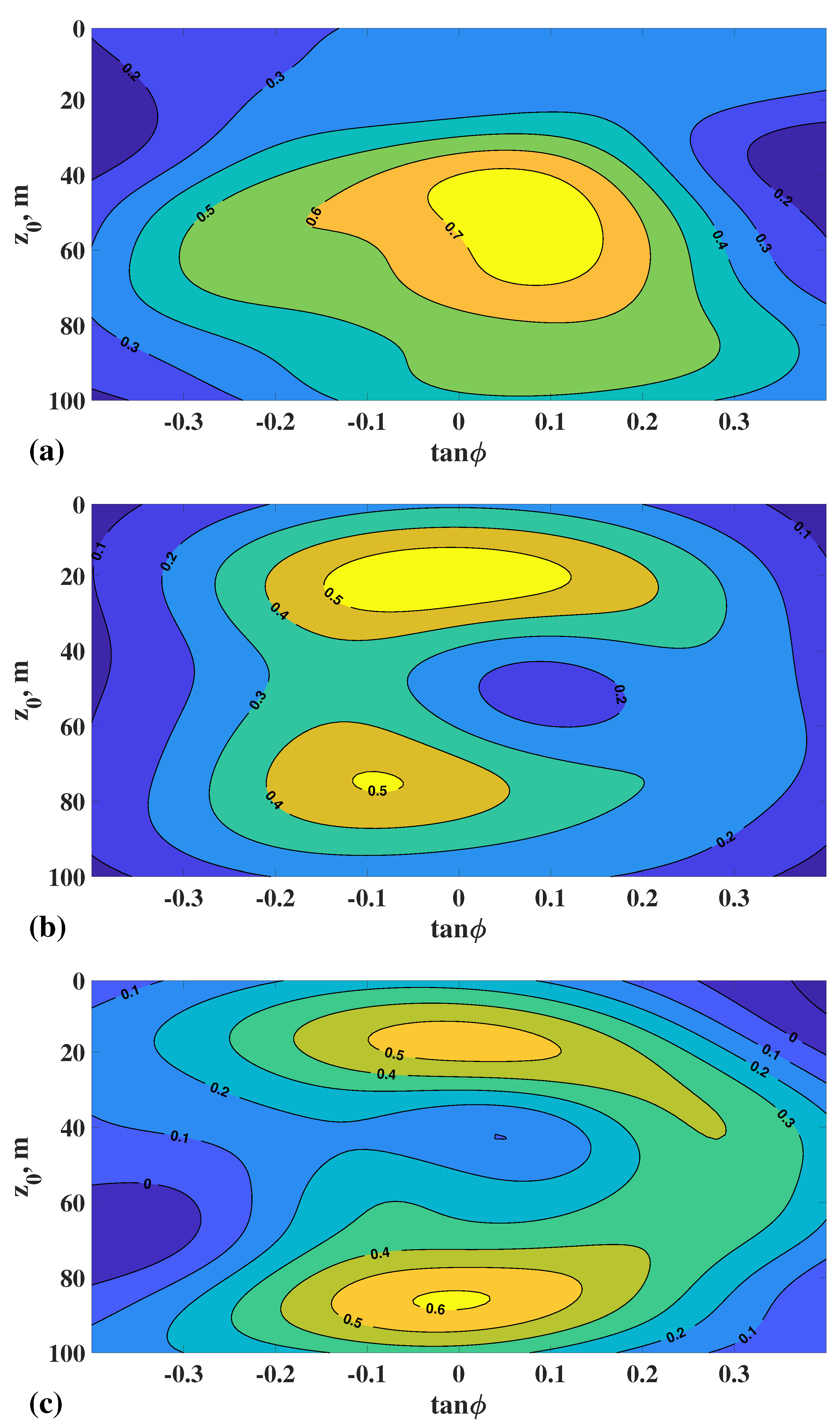
In the present paper, we consider wavefields with frequencies from 100 to 300 Hz. This frequency range corresponds to relatively weak bottom losses and therefore is more suitable for remote sensing of gas-saturated areas. The propagation distance R is 10 km. Figure 2 demonstrates the colour diagram of the transmission coefficient for the waveguide without pockmarks for $f=100$ Hz. In the absence of ambient noise, one can see the symmetric pattern that is typical for range-independent waveguides, as it is shown in the panel (a). Noise destroys the symmetry, with marked prevalence of the downgoing ($\tan \varphi >0$) component of the acoustic energy flux.

The presence of a large pockmark leads to cardinal changes in the diagram pattern. Figure 3 illustrates data for the pockmark occupying the waveguide segment between $r_1=2000$ m and $r_2=2300$ m. As it was mentioned in the Introduction, pockmarks with such sizes can be referred to as giant pockmarks. As it follows from Figure 3a, only beams with initial conditions near $z_0=55$ m and $\tan \varphi =0.08$ are weakly affected by the pockmark. Apparently trajectories of these beams “jump over” the pockmark. Other beams are strongly attenuated as compared to the data without the pockmark. To highlight the changes, we also plot the difference

$$\delta T(\tan \varphi ,z_0)=T_{\mathrm{ref}}(\tan \varphi ,z_0)-T_{\mathrm{pockmark}}(\tan \varphi ,z_0),$$

(33)

where $T_{\mathrm{ref}}$ corresponds to the reference waveguide without the pockmark, and $T_{\mathrm{pockmark}}$ is calculated with the pockmark. Peaks of this function allows one to pick out the most attenuated wave beams. The difference $\delta T(\tan \varphi ,z_0)$ is demonstrated in Figure 3b,c.

In the absence of noise (see Figure 3b) one can see two well resolved peaks: one near $z=20$ m, and another one near $z=80$ m. Noise with $\sigma =\sqrt{0.05}$ doesn’t blur these peaks (see Figure 3c). Influence of the pockmark on the beam emitted with $z_0=80$ m and $\tan \varphi =-0.1$ is illustrated in Figure 4: the pockmark opens the channel for acoustic energy flux into the bottom and thereby strongly reduces intensity as compared to the case without the pockmark. Nevertheless, one can see that the beam is not absorbed by the pockmark completely, and the remaining part has the form of the aforementioned “jump-over” mode.

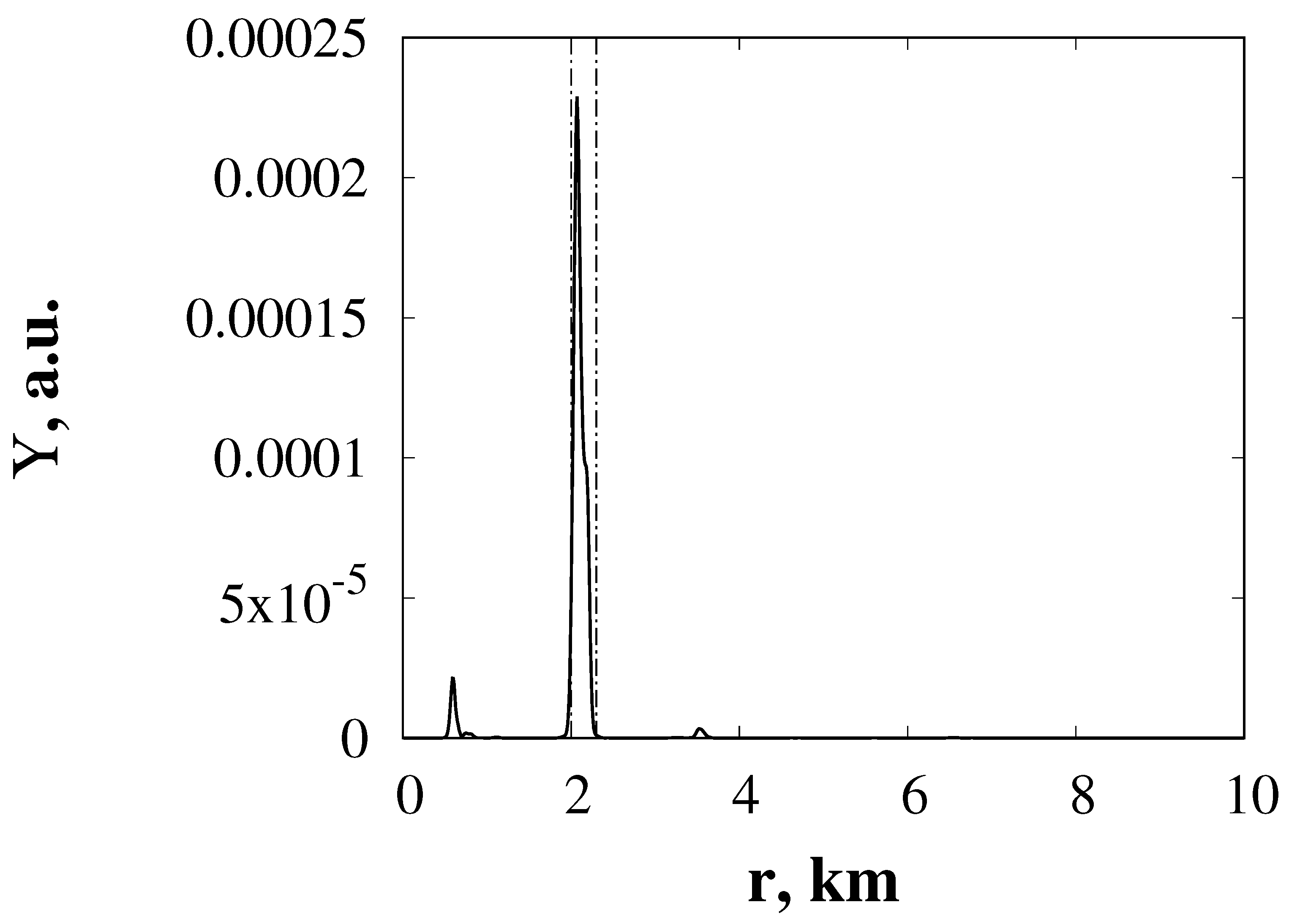
Provided the background hydrology and bathymetry are known, the presence of separate peaks of the function $\delta T(\tan \varphi ,z_0)$ gives an opportunity to estimate probable location of the pockmark relying upon the data of scanning. It is reasonable to assume that simultaneous attenuation of these beams implies their contact with the pockmark at nearly the same regions. It anticipates that their intersections in the close vicinity of the bottom could be considered as possible locations of the pockmark. Unfortunately, ray tracing cannot give accurate estimates for such low signal frequencies. Therefore, one needs full-wave analysis for finding beam intersections. Basically, peaks of the function $\delta T(\tan \varphi ,z_0)$ depend on frequency; therefore, one can trace out simultaneous near-bottom intersections of large number of absorbed beams corresponding to various frequencies: they all should intersect in the vicinity of the pockmark. Then, the most probable locations of the pockmark can be found as peaks of the following overlap function:

$${\rm Y}\left(r\right)=\underset{h-\delta h}{\overset{h}{\int }}\prod _{n=1}^N{\left|{\Psi }^{\left(n\right)}(z,r,f_n)\right|}^{2}dz,$$

(34)

where N is the number of absorbed beams taken into account, ${\Psi }^{\left(n\right)}(r,z,f_n)$ the nth absorbed beam, $\delta h=15$ m. Now, let us simulate an experiment and assume that background characteristics (sound speed and salinity fields, background sediment density etc.) of the waveguide are known, but apriori information about location of the pockmark is lacking. Then, one can compute the beam wavefields for the background waveguide, i.e., without the pockmark, and find the peaks of the overlap function (34). It was found that number of candidate peaks is reduced with increasing of N. According to Figure 5, there is one dominant peak for $N=14$, and its location coincides with the actual location of the pockmark. Fourteen beams used for this calculation correspond to different absorption spots obtained via the scanning of the transmission coefficient T for frequencies 100, 150, 200, 250, and 300 Hz.

Form and position of absorption peaks in the diagrams like those are depicted in Figure 3 depend on the distance from the pockmark to the arrays. Figure 6 illustrates results of scanning for the pockmark crossing the waveguide between $r_1=8000$ m and $r_2=8300$ m, i.e., placed not far from the receiving array. As it is shown in Figure 6a, the “jump-over” mode corresponds to the family of beams emitted with small upward inclination from the depth interval near $z=30$ m. In the absence of noise, one can see one broad absorption peak presented in Figure 6b. This absorption peak splits into a pair as noise is added (see Figure 6c).

As in the preceding case, one can try to find the pockmark location by calculating the overlap function for absorbed beams. According to Figure 7, overlap of 16 absorbed beams allows one to unambiguously determine the pockmark location: we have the dominant peak of ${\rm Y}$ at the pockmark. This gives hope for the successful determination of the position of the pockmark based on the results of acoustic scanning.

5. Discussion

The subject of the present work is remote identification of gas-saturated sediments by means of low-frequency acoustic scanning. We develop a new method that can be used in marine expeditions for studying gassy sediment areas, which are permeable for upward gas migration through the lythosphere.

Particularly, we consider the case of gassy sediments corresponding to active pockmarks. It is shown that measurement of the wavefield propagator allows us to identify the presence of such sediments by means of proper processing of measured data. In fact, we utilize a kind of wave shouting and identify the most sensitive (i.e., significantly absorbed) and the most insensitive (the “jump-over” mode) wavepackets. If one has enough information about environment and can model the geometry of wavepacket propagation, then it is possible to find the most probable locations of the pockmark. Of course, the location results are very sensitive to the accuracy of the information about the background medium. If such information is lacking, our method can be considered only as an auxiliary tool to facilitate pockmark location by means of traditional techniques based on direct bottom ensonification from a vessel, like the continuous seismic profiling. Once the pockmark presence in a particular direction is established, the vessel can explore the corresponding propagation path with the continuous seismic profiling and find the pockmark.

The procedure of the propagator measurement by means of two vertical arrays, one transmitting and another one receiving, is relatively complicated. Therefore, it is reasonable to develop a simpler method. For example, we can try to use the basis of the so-called discrete variable representation (DVR) functions, using the ideas formulated in [29,34]. These functions form the orthonormal basis and also can be used for measurement of the propagator. Each DVR function can be excited by only one monopole, i.e., a single point source can be enough for measurement.

We consider the case of a giant pockmark spanning over 300-m long segment of a waveguide. However, the approach presented can be also implemented to smaller zones of gas emission. In that case, signals with higher frequencies might be better option. It is worth reminding that the model of a waveguide considered in this paper is idealistic. First, we do not consider horizontal refraction that could impede robust measurement of the propagator. Second, we neglect spatial inhomogeneities in the bottom relief, sound speed field, and medium density. The acoustical model of a pockmark should be more complicated. So, it is important to examine the approach presented in this paper with a realistic model of environment. On the other hand, it is reasonable to expect that usage of broadband pulses instead of tonal signals should increase amount of information obtained by means of the acoustic scanning. In this case, dispersive properties of the sediment could be important. We hope to address these issues in the forthcoming work. Further development of this approach can lead to a new powerful method for remote mapping of hydrocarbon provinces.

6. Conclusions

The main result is a novel approach for acoustic remote sensing for bottom anomalies associated with extensive gas emission. The case of an anomaly caused by a giant pockmark is taken as an example. The approach is based on measurement of acoustic propagator. Complementing this measurement with numerical simulation involving virtual acoustic scanning, one can analyze differences in beam loss and thus estimate the possible location of the pockmark. Numerical simulation presented in this paper involves scanning of the waveguide with Gaussian beams, with subsequent analysis of their attenuation. It is shown that the approach can work fairly in the presence of moderate noise. Usage of such approach can significantly facilitate search of emission zones.