Article

Angular Spectrum of Acoustic Pulses at Long Ranges

by
Denis V. Makarov
* and
Leonid E. Kon’kov
V.I. Il’ichev Pacific Oceanological Institute of the Far-East Branch of the Russian Academy of Sciences, 690041 Vladivostok, Russia
*
Author to whom correspondence should be addressed.
J. Mar. Sci. Eng. 2023, 11(1), 29; https://doi.org/10.3390/jmse11010029
Submission received: 20 November 2022 / Revised: 8 December 2022 / Accepted: 17 December 2022 / Published: 27 December 2022
(This article belongs to the Special Issue Sound Scattering in the Ocean)

Abstract

:
Long-range propagation of sound pulses in the deep ocean is considered. A new method for the estimation of the pulse angular spectrum is presented. The method is based on the Husimi transform of a wave field and can be realized with a short vertical array of nondirectional hydrophones. As a result, one obtains a diagram of the arrival pattern in the time–angle plane. The method is applied to a model of the underwater sound channel in the Sea of Japan. Special attention is paid to sound scattering on a cold synoptic eddy along the waveguide. It is shown that the synoptic eddy leads to a splitting of the individual ray’s arrivals into clusters with close angles and times. The random sound-speed perturbation induced by internal waves blurs these clusters into a fuzzy background and simultaneously broaden the angular spectrum of pulses. Nevertheless, it is found that the latter effect is relatively weak for short vertical arrays. In particular, it is shown that increasing the array length from 10 to 30 m results in the separation of the arrivals with opposite angles.

1. Introduction

Sound scattering on internal waves has long ago been recognized as the main source of signal decoherence for long-range sound propagation in the ocean. Although internal-wave-induced sound-speed variations are commonly very weak, their accumulated effect on ranges of a few hundred kilometers is very meaningful. Mechanisms of decoherence for frequencies above 50 Hz are well-described within the theory of wave chaos [1]. The term wave chaos is usually understood as manifestations of the Lyapunov instability of ray trajectories in wave dynamics. The instability comes from the fundamental nonintegrability of Hamiltonian ray equations in an inhomogeneous waveguide. Lyapunov instability makes ray trajectories highly irregular and expects disordered interference patterns for relatively high acoustic frequencies.
The study of wave chaos in ocean acoustics is important from the viewpoint of various applications. Earlier chaos was considered as the main factor that impeded the reconstruction of oceanic environments by means of hydroacoustical tomography [2]. Later, it was argued that chaos could enhance sensitivity to large-scale inhomogeneities [3,4] and thereby play a positive role in the context of tomography. In particular, the analysis of chaos-assisted modal pulse elongation may allow one to estimate the depth of a synoptic eddy that crosses a waveguide. Moreover, it is recognized that chaos-assisted phenomena are a major consideration in long-range underwater acoustic communication, in which the scattering on internal waves causes a significant coherence loss [5,6,7,8].
The present work is devoted to the influence of the scattering on internal waves onto the angular structure of acoustic pulses. The analysis of the angular spectrum can be worthy from the viewpoint of source identification [9,10]. The approach proposed in this paper is a simplified version of the method developed in [11]. It is based on a phase-space picture of a wave field and takes into account the fundamental limitations on the measurement of arrival angles. Our attention is concentrated on arrival angles in the vertical plane, which are closely related to the modal spectrum of a wave field. Nevertheless, the same approach can be readily implemented for horizontal arrays and angles as well.

2. Theory

Considering long-range sound propagation, one can neglect the contribution from sound waves contacting with the lossy bottom. Therefore, it is possible to utilize the small-angle approximation that yields the standard parabolic equation for a wave-field envelope Ψ . Following [11,12], the standard parabolic equation can be expressed in the operator form
i k 0 Ψ r = H ^ Ψ ,
where r is the range, k 0 = 2 π f / c 0 , f is the signal frequency, c 0 is the reference sound speed,
H ^ = p ^ 2 2 + V ( z , r )
is the Hamiltonian operator, and
p ^ = i k 0 z , V ( z , r ) = c ( z , r ) c 0 1 .
The wave-field envelope is related to the acoustic pressure u by means of the formula
Ψ = π k 0 r 2 e i ( k 0 r π 4 ) u .
The operator presentation reveals the mathematical equivalence between the standard parabolic equation and the Schrödinger equation in quantum mechanics. In this analogy, range r plays the role of a timelike variable, p ^ acts as the momentum operator, and V is the potential energy. In the short-wavelength limit being the analogue of the semiclassical limit in quantum mechanics, the Hamiltonian operator (2) becomes the classical Hamiltonian
H ^ = p 2 2 + V ( z , r ) ,
where
p = n sin χ tan χ
is the so-called ray momentum, and χ is the ray grazing angle. The corresponding ray equations are
d z d r = H p = p , d p d r = H z .
Variables z and p act as coordinates in the ray-based phase space. The projection of a wave field onto this space is provided by the Wigner transform defined as
W ( p , z , k 0 ) = k 0 2 π A d ζ Ψ ( z ζ / 2 , k 0 ) Ψ * ( z + ζ / 2 , k 0 ) e i k 0 p ζ ,
where the constant A is the norm of the wave function
A = | Ψ ( z ) | 2 d z .
The Wigner function W can be thought of as the quasi-probability density in the space of ray variables z and p. Taking into account (6), one can consider the dependence of the Wigner function on p for fixed z and k 0 as a kind of local angular wave-field spectrum.
However, the Wigner function can exhibit fast oscillations due to the interference that could be inconvenient for its analysis. Therefore, it is reasonable to replace the Wigner function by its coarse-grained analogue [13,14],
W sm ( p , z , k 0 ) = 1 2 π d z d p exp ( z z ) 2 2 Δ z 2 ( p p ) 2 2 Δ p 2 W ( z , p ) .
Another difficulty arising in the analysis of the angular spectrum by means of the Wigner transform can be well-understood from the viewpoint of the aforementioned equivalence between parabolic and Schrödinger equations. It is well-known that quantum mechanical uncertainties in the simultaneous measurement of the position and momentum obey the celebrated Heisenberg relation. This relation ensues from the basic properties of wave fields and therefore can be readily adopted in ocean acoustics. The acoustical version of the Heisenberg relation reads [3,11]
Δ z Δ p 1 2 k 0 ,
where Δ p can be referred to as the angular uncertainty. This limitation has a fundamental origin and is not linked to imperfect conditions of signal reception. The relation (11) links the angular uncertainty with the array length: the longer the array, the smaller the uncertainty. Moreover, it puts a constraint onto physically relevant values of smoothing scales in (10). The case of the minimal uncertainty
Δ z Δ p = 1 2 k 0
corresponds to the so-called Husimi function
W H ( p , z , k 0 ) = 1 A Δ z 2 π Ψ * ( z , k 0 ) exp i k 0 p ( z z ) ( z z ) 2 4 Δ z 2 d z 2 .
In the context of sound propagation in the ocean, the Husimi function was utilized in [3,11,15,16,17,18]. Some of its properties could be used for the analysis of chaos manifestations in a wave-field structure [17,19,20,21].
Wigner and Husimi functions provide a ray-based interpretation of a continuous wave field. However, acoustical experiments are commonly conducted with pulsed broadband signals. A generalization of the Husimi function onto pulse wave fields was obtained in [11]. It was based on the proper time-domain Fourier decomposition of the pulse. Unfortunately, a practical implementation of this procedure may lead to additional inaccuracy due to the impact of the noise that affects signal waveforms. Nevertheless, if the signal spectrum has a peak at some frequency f ¯ , one can avoid the time-domain Fourier decomposition by replacing k 0 in (13) by k ¯ 0 = 2 π f ¯ / c 0 and then applying the Husimi transform to the time front of the received signal
Ψ ˜ ( z , t ) = S ( f ) Ψ ( z , r , f ) e i [ k 0 ( f ) R 2 π f t ] d f ,
where S ( f ) is the signal spectrum, and R is the distance between the source and the receiver. This yields
W ˜ H ( p , z , t ) = 1 A Δ z 2 π Ψ ˜ * ( z , t ) exp i k ¯ 0 p ( z z ) ( z z ) 2 4 Δ z 2 d z 2 .
The estimation of the angular pulse spectrum via Equation (15) is the main approach used in this paper. This formula is an approximate version of the exact expression presented in [11].
If one has an equidistant vertical array of hydrophones at depths z = z 1 , z 2 , , z N , where z n = z 1 + ( n 1 ) d z , then Formula (15) reads as
W ˜ H ( p , z , t ) = 1 A discr Δ z 2 π n Ψ ˜ * ( z n , t ) exp i k ¯ 0 p ( z n z ) ( z n z ) 2 4 Δ z 2 2 ,
provided the hydrophone spacing d z is small compared to the smallest vertical wavelength λ = c 0 / ( f ¯ p max ) 3 c 0 / f ¯ . The constant A discr is given by
A discr = n | Ψ ( z n ) | 2 .
Alternatively, one can reconstruct a continuous wave field profile by means of the techniques proposed in [22] and then apply the transform (15).
Thus, one can specify some depth as a center of a receiving antenna and calculate the arrival-time-dependent angular spectrum at this point by means of the Husimi transform (16). Taking into account that the Husimi function corresponds to a Gaussian coarse-graining of the Wigner function (8), it turns out that the Husimi processing of a signal can be readily produced with an antenna length of 6 Δ z .

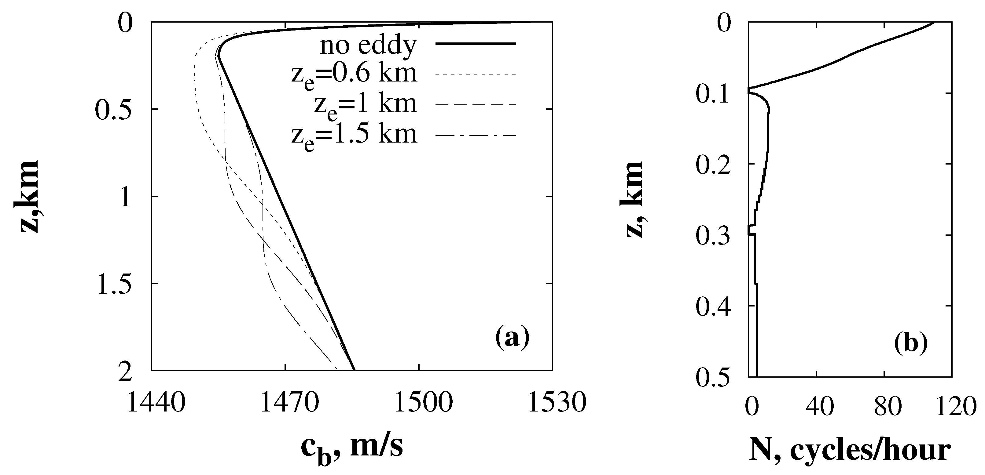
3. Model of a Waveguide

Let us consider a deep-water acoustic waveguide where the function V ( z , r ) is given by the sum
V ( z , r ) = 1 + c b ( z ) c 0 + V eddy + V iw ,
where c b ( z ) is a background range-independent sound-speed profile, V eddy and V iw are perturbations contributed from the synoptic eddy and internal waves, respectively. In the numerical simulation, we used a model of the underwater sound channel in the Sea of Japan. The background sound-speed profile is described by the formula [4,12]
c b ( z ) c 0 + Δ c ( z ) = c 0 + Δ c up ( z ) , z z 0 , c 0 + Δ c low ( z ) , z > z 0 .
where
Δ c up ( z ) = c 1 e z / B , Δ c low ( z ) = c 1 e z 0 / B + g ( z z 0 ) ,
and c 0 = 1455 m/s, c 1 = 70 m/s, z 0 = 200 m was the depth of the waveguide axis, corresponding to the minimum of the sound speed, B = 30 m was the thermocline depth, and g = 0.017 s−1. The ocean bottom was assumed to be flat and located at a depth of 3 km. The upper part of the background sound-speed profile is shown in Figure 1a as a solid line. It should be noted that a similar profile was considered in Ref. [23] devoted to the propagation of explosion-produced signals in the Sea of Japan.
We considered two factors of horizontal inhomogeneity: a synoptic eddy and internal waves. The sound-speed perturbation caused by the synoptic eddy is given by the following formula [1,24,25]:
V eddy = c e c 0 exp ( r r e ) 2 Δ r 2 ( z z e ) 2 Δ Z ( r ) 2 ,
where
Δ Z ( r ) = Δ z c Δ z υ exp ( r r υ ) 2 Δ r υ 2 .
We used the following set of parameter values: c e = 10 m/s, r e = 100 km, Δ r = 50 km, Δ z c = 500 m, Δ z υ = 250 m, r υ = 120 km, and Δ r υ = 20 km. The numerical simulation was carried out for the eddies with core depths z e varying from 600 to 1500 m. The respective sound-speed profiles are depicted in Figure 1a. All the curves presented correspond to r = r e , where the eddy-induced distortion of a profile is the strongest.
The sound-speed perturbation induced by internal waves is given by the formula [26]
δ c iw ( z , r ) = c b ( z + ζ ( z , r ) ) c b ( z ) ,
where ζ is the vertical displacement of a fluid parcel. We constructed ζ ( z , r ) as a modal superposition using the approach presented in [27]. The Väisäla–Brunt (buoyancy) frequency profile was calculated by means of hydrological data for the Sea of Japan [28]. The method of calculation is described in detail in Ref. [4]. The resulting profile is presented in Figure 1b. Notably, the buoyancy frequency is very large in the near-surface layer and is almost zero below it. It turns out that a waveguide for internal waves is too narrow and can efficiently focus only on a low number of internal-wave modes. This results in weakness of the vertical oscillations of the corresponding sound-speed perturbation. A statistical analysis of an internal-wave field confirmed it. As in [4], we utilized the expansion over empirical orthogonal functions f n ( z )
δ c iw ( z , r ) = < δ c iw ( z ) > + n b n ( r ) f n ( z ) .
Functions f n ( z ) can be found as the eigenvectors of the covariance matrix K ^ with entries
K i j = 1 l max l = 1 l max [ δ c iw , l ( z i ) < δ c iw ( z i ) > ] × [ δ c iw , l ( z j ) < δ c iw ( z j ) > ] ,
where the index l enumerates l max statistically independent realizations of δ c iw ( z ) , and { z i } is a discrete set of depth values that is used to represent δ c iw ( z ) as a vector. The angular brackets correspond to averaging over realizations. Taking into account the oscillating form of δ c iw , it is reasonable to set < δ c iw > = 0 .
The eigenvalues of K ^ evaluate the contributions of the corresponding eigenvectors in the sum (24). They rapidly decrease in value as their number increases, and the first two eigenfunctions accumulate about 90 percent of the overall power. This circumstance reflects weakness of the high-order modes of internal waves which are mainly responsible for the vertical oscillations of the sound-speed perturbation. As it was shown in [1,17,29,30], these vertical oscillations play a primary role in the emergence of strong chaos for almost flat near-axial rays. These rays form the last portion of the received pulse (see, for example, [31]). Consequently, the underwater sound channel in the Sea of Japan implies a regular propagation near the waveguide axis. This expectation is well confirmed both numerically [12] and experimentally [32,33].

4. Results

In the numerical simulation, pulses of the following form were considered:
s ( t ) = exp 2 π i f 0 t 2 π 2 Δ f 2 t 2 .
The pulse spectrum was given by
S ( f ) = 1 2 π Δ f exp ( f f 0 ) 2 2 Δ f 2 .
We considered the case of f 0 = 300 Hz and Δ f = 60 Hz. The initial wave packet was chosen as
Ψ 0 ( z ) = exp ( z z s ) 2 4 σ z 2 ,
where z s = 200 m and σ z = 50 m. The distance between the source and receiver, R, was taken as 350 km.
The parabolic Equation (1) was solved numerically for a frequency interval from 20 to 500 Hz with a step of 0.2 Hz. Husimi functions were computed via Formula (16) and averaged over 100 realizations of the internal wave field. The vertical spacing between hydrophones, d z , was taken as 1 m. Figure 2 represents the plots of the Husimi function with a coarse-graining scale Δ z = 10 m. The corresponding angular uncertainty Δ p was 0.039. It was assumed that the receiving array was centered at the waveguide axis, z = z 0 = 200 m. The Husimi plot corresponding to the waveguide without the synoptic eddy demonstrates arrivals which are well-resolved in time but looked smeared in angle. It is illustrated in Figure 2a. The angular smearing is a consequence of the limitations posed by the Heisenberg uncertainty relation (11). It leads to a partial overlapping of the branches corresponding to positive and negative arrival angles. Nevertheless, individual arrivals corresponding to both branches are well identified.
The onset of an eddy along the waveguide complexifies the arrival pattern, as is shown in Figure 2b–d. As long as we consider the case of a cold eddy giving rise to a negative variation of the sound speed, the Husimi diagram is moved to larger arrival times. In the absence of scattering on internal waves, individual arrivals were split into weaker ones. It is demonstrated in Figure 2f–h. The weakest arrivals are unstable in the presence of the random inhomogeneity, so the statistical averaging blurs them to a fuzzy continuous background. It should be emphasized that travel times for stronger arrivals sometimes do not coincide with those in the absence of the random inhomogeneity. This indicates the importance of incorporating internal waves into the acoustic models of long-range sound propagation.
It has to be noted that the temporal smearing is nonuniform. There is tendency of decreasing times corresponding to the most smeared segment when increasing the core depth. It means that a deeper eddy affects steeper rays, causing a local enhancement of ray chaos. This issue is discussed in detail in [4].
Increasing the smoothing scale Δ z to 30 m should correspond to a triple elongation of the array. In this case, the angular uncertainty Δ p is reduced to 0.013. The corresponding angular structure is illustrated in Figure 3. A reduction of the angular uncertainty makes the branches corresponding to positive and negative arrival angles almost nonoverlapping. Indeed, decreasing the angular uncertainty does not influence the temporal smearing but provides a more accurate estimate of the arrival angles corresponding to the smeared segments, that is, one can accurately identify ray bunches which were the most affected by scattering on an eddy. This is desirable from the viewpoint of hydroacoustical tomography. In a more general context, the improvement of angular resolution allows one to identify the corresponding ray “skeleton” of a wave field that facilitates the solution of various practical problems. The requirement of a sufficient angular resolution imposes a constraint on the array length, as the latter one is the main factor determining the maximum possible Δ z .

5. Discussion

The manuscript addressed the problem of the arrival angle identification in underwater acoustics. As in [11], we underlined the importance of the fundamental Heisenberg limitation on angle measurements. This limitation is associated with a finiteness of the array length and leads to an inherent uncertainty in the angular spectrum. In the case of long-range sound propagation, the Heisenberg uncertainty is accompanied by a broadening of the angular spectrum due to the sound scattering on internal waves. Nevertheless, the results of numerical simulation showed that the broadening of the angular spectrum was much less significant than the temporal pulse elongation. The latter circumstance is important from the viewpoint of hydroacoustical tomography. Indeed, signal travel times are very sensitive to large-scale variability of the ocean. Overall timefront shifts were caused by the cold synoptic eddies, while individual timefront branches were smeared due to the scattering on internal waves. The results of Ref. [14] suggest that such smeared patterns may be more efficiently reproduced by means of ray calculations based on the incoherent summation of ray bundles. This ensues from the fact that bundles consisting of a large number of rays are much less affected by ray chaos caused by scattering on internal waves [1]. Such an elimination of the ray chaos outlines the prospect for the development of an efficient scheme for hydroacoustical tomography. We hope to address this issue in forthcoming works.
The angular broadening can be controlled by the depth uncertainty Δ z . As long as Δ z is linked to the array length, one can conclude that the array elongation can substantially facilitate a ray-based interpretation of an arrival pattern. On the other hand, we have to keep in mind that this result was obtained for the Sea of Japan, where sound scattering on internal waves is relatively weak due to a weak impact of high-order internal wave modes [12]. It is reasonable to expect that marine environments with a broader vertical wavenumber spectrum should give rise to more complicated angular patterns. Another promising issue is the analysis of the angular spectrum of acoustic noise wave fields [34,35,36].

6. Conclusions

In the present work, we developed a simple method for the analysis of acoustic pulses by means of a relatively short antenna with nondirectional hydrophones. The method involves the analysis of angular and temporal pulse characteristics simultaneously. It is based on the Husimi transform being a projection of a wave field onto the phase space of ray equations. Thus, one can obtain a raylike interpretation of arrival patterns without direct ray calculations.
A model of the underwater sound channel in the Sea of Japan was considered as an example. Particular attention was paid to the influence of synoptic eddies onto the arrival pattern. It was shown that sound scattering on an eddy resulted in a splitting of individual arrivals into groups. Scattering on random internal-wave-induced inhomogeneity blurs the groups of low-amplitude arrivals. It was pointed out that the temporal interval of the strongest blurring depended on the depth of the eddy core. Increasing the depth uncertainty results in a separation of the arrivals with opposite angles, with the onset of a raylike arrival pattern. This result suggests that a successful identification of propagation paths in terms of ray trajectories requires a sufficient array length.

Author Contributions

Conceptualization, D.V.M.; methodology, D.V.M.; software, L.E.K.; validation, L.E.K.; formal analysis, D.V.M.; investigation, L.E.K. and D.V.M.; resources, L.E.K.; data curation, L.E.K.; writing—original draft preparation, D.V.M.; writing—review and editing, D.V.M.; visualization, L.E.K.; supervision, D.V.M.; project administration, D.V.M. All authors have read and agreed to the published version of the manuscript.

Funding

The authors acknowledge support from the Laboratory of Nonlinear Hydrophysics and Natural Hazards of V.I. Il’ichev Pacific Oceanological Institute, Far Eastern Branch Russian Academy of Sciences, project of Ministry of Science and Education of Russia, agreement no. 075–15-2022–1127.

Institutional Review Board Statement

Not applicable.

Informed Consent Statement

Not applicable.

Data Availability Statement

Not applicable.

Acknowledgments

The authors are grateful to A.L. Virovlyansky and P.S. Petrov for fruitful discussions in the course of this research.

Conflicts of Interest

The authors declare no conflict of interest.

References

  1. Makarov, D.; Prants, S.; Virovlyansky, A.; Zaslavsky, G. Ray and Wave Chaos in Ocean Acoustics: Chaos in Waveguides; Series on Complexity, Nonlinearity and Chaos; World Scientific: Singapore, 2010. [Google Scholar]
  2. Tappert, F.D.; Tang, X. Ray chaos and eigenrays. J. Acoust. Soc. Am. 1996, 99, 185–195. [Google Scholar] [CrossRef]
  3. Smirnov, I.P.; Virovlyansky, A.L.; Edelman, M.; Zaslavsky, G.M. Chaos-induced intensification of wave scattering. Phys. Rev. E 2005, 72, 026206. [Google Scholar] [CrossRef] [PubMed]
  4. Makarov, D.V.; Kon’kov, L.E.; Petrov, P.S. Influence of oceanic synoptic eddies on duration of modal acoustic pulses. Radiophys. Quantum Electron. 2016, 58, 1–15. [Google Scholar] [CrossRef]
  5. Virovlyansky, A.L.; Kazarova, A.Y.; Lyubavin, L.Y. Focusing of sound pulses using the time reversal technique on 100-km paths in a deep sea. Acoust. Phys. 2012, 58, 678–686. [Google Scholar] [CrossRef]
  6. Yao, H.; Wang, H.; Xu, Y.; Kurths, J. A recurrent plot based stochastic nonlinear ray propagation model for underwater signal propagation. New J. Phys. 2020, 22, 063025. [Google Scholar] [CrossRef]
  7. Makarov, D.V.; Komissarov, A.A. Modelling of sound propagation in the ocean using the matrix propagator. Proc. Meet. Acoust. 2020, 42, 055004. [Google Scholar] [CrossRef]
  8. Huang, J.; Diamant, R. Adaptive Modulation for Long-Range Underwater Acoustic Communication. IEEE Trans. Wirel. Commun. 2020, 19, 6844–6857. [Google Scholar] [CrossRef]
  9. Virovlyansky, A.L.; Kazarova, A.Y.; Kenigsberger, G.V.; Kolodiev, O.V.; Korotin, P.I.; Lyubavin, L.Y.; Moiseenkov, V.I.; Orlov, D.A.; Potapov, O.A.; Turchin, V.I. Experiment on estimating the coordinates of an emitter on the Black Sea shelf. Acoust. Phys. 2015, 61, 196–204. [Google Scholar] [CrossRef]
  10. Dubrovinskaya, E.; Kebkal, V.; Kebkal, O.; Kebkal, K.; Casari, P. Underwater Localization via Wideband Direction-of-Arrival Estimation Using Acoustic Arrays of Arbitrary Shape. Sensors 2020, 20, 3862. [Google Scholar] [CrossRef] [PubMed]
  11. Makarov, D. On measurement of acoustic pulse arrival angles using a vertical array. Acoust. Phys. 2017, 63, 673–680. [Google Scholar] [CrossRef]
  12. Makarov, D.V.; Kon’kov, L.E.; Uleysky, M.Y.; Petrov, P.S. Wave chaos in a randomly inhomogeneous waveguide: Spectral analysis of the finite-range evolution operator. Phys. Rev. E 2013, 87, 012911. [Google Scholar] [CrossRef] [PubMed] [Green Version]
  13. Virovlyanskii, A.L.; Okomel’kova, I.A. The ray approach to calculation of the local spectrum of a field in a waveguide smoothed over the angular and spatial scales. Radiophys. Quantum Electron. 1997, 40, 1039–1047. [Google Scholar] [CrossRef]
  14. Virovlyansky, A.L.; Zaslavsky, G.M. Evaluation of the smoothed interference pattern under conditions of ray chaos. Chaos Interdiscip. J. Nonlinear Sci. 2000, 10, 211–223. [Google Scholar] [CrossRef] [PubMed]
  15. Sundaram, B.; Zaslavsky, G.M. Wave analysis of ray chaos in underwater acoustics. Chaos 1999, 9, 483–492. [Google Scholar] [CrossRef] [PubMed]
  16. Smirnov, I.P.; Virovlyansky, A.L.; Zaslavsky, G.M. Wave chaos and mode–medium resonances at long-range sound propagation in the ocean. Chaos 2004, 14, 317–332. [Google Scholar] [CrossRef]
  17. Kon’kov, L.E.; Makarov, D.V.; Sosedko, E.V.; Uleysky, M.Y. Recovery of ordered periodic orbits with increasing wavelength for sound propagation in a range-dependent waveguide. Phys. Rev. E 2007, 76, 056212. [Google Scholar] [CrossRef] [PubMed] [Green Version]
  18. Makarov, D.V.; Kon’kov, L.E.; Uleysky, M.Y. Wave chaos in underwater acoustics. J. Sib. Fed. Univ. Math. Phys. 2010, 3, 336–348. [Google Scholar]
  19. Sugita, A.; Aiba, H. Second moment of the Husimi distribution as a measure of complexity of quantum states. Phys. Rev. E 2002, 65, 036205. [Google Scholar] [CrossRef] [Green Version]
  20. Arranz, F.J.; Seidel, L.; Giralda, C.G.; Benito, R.M.; Borondo, F. Onset of quantum chaos in molecular systems and the zeros of the Husimi function. Phys. Rev. E 2013, 87, 062901. [Google Scholar] [CrossRef] [Green Version]
  21. Oregi, I.; Arranz, F.J. Distribution of zeros of the Husimi function in systems with degeneracy. Phys. Rev. E 2014, 89, 022909. [Google Scholar] [CrossRef]
  22. Makarov, D.; Petrov, P. Full reconstruction of acoustic wavefields by means of pointwise measurements. Wave Motion 2022, 115, 103084. [Google Scholar] [CrossRef]
  23. Vadov, R.A. Point-source field in the underwater sound channel of the Sea of Japan. Acoust. Phys. 1998, 44, 516–523. [Google Scholar]
  24. Virovlyansky, A.L.; Kazarova, A.Y.; Lyubavin, L.Y. The possibility of using a vertical array for estimating the delays of sound pulses at multimegameter ranges. Acoust. Phys. 2008, 54, 486–494. [Google Scholar] [CrossRef]
  25. Virovlyansky, A.L.; Kazarova, A.Y.; Lyubavin, L.Y. Estimation of distortions in the sound field propagating through mesoscale inhomogeneities. Acoust. Phys. 2010, 56, 317–327. [Google Scholar] [CrossRef]
  26. Godin, O.; Zavorotny, V.; Voronovich, A.; Goncharov, V. Refraction of Sound in a Horizontally Inhomogeneous, Time-Dependent Ocean. IEEE J. Ocean. Eng. 2006, 31, 384–401. [Google Scholar] [CrossRef]
  27. Colosi, J.A.; Brown, M.G. Efficient numerical simulation of stochastic internal-wave-induced sound-speed perturbation fields. J. Acoust. Soc. Am. 1998, 103, 2232–2235. [Google Scholar] [CrossRef]
  28. Rostov, I.D.; Yurasov, G.I.; Rudykh, N.I.; Dmitrieva, E.V.; Rostov, V.I. Electronic oceanographic atlas of the Bering Sea and the Seas of Okhotsk and Japan. Oceanology 2004, 44, 439–444. [Google Scholar]
  29. Virovlyansky, A.L.; Makarov, D.V.; Prants, S.V. Ray and wave chaos in underwater acoustic waveguides. Phys.-Uspekhi 2012, 55, 18–46. [Google Scholar] [CrossRef]
  30. Makarov, D.V.; Kon’kov, L.E.; Uleysky, M.Y. The ray-wave correspondence and the suppression of chaos in long-range sound propagation in the ocean. Acoust. Phys. 2008, 54, 382–391. [Google Scholar] [CrossRef]
  31. Beron-Vera, F.J.; Brown, M.G.; Colosi, J.A.; Tomsovic, S.; Virovlyansky, A.L.; Wolfson, M.A.; Zaslavsky, G.M. Ray dynamics in a long-range acoustic propagation experiment. J. Acoust. Soc. Am. 2003, 114, 1226–1242. [Google Scholar] [CrossRef] [Green Version]
  32. Spindel, R.C.; Na, J.; Dahl, P.H.; Oh, S.; Eggen, C.; Kim, Y.G.; Akulichev, V.A.; Morgunov, Y.N. Acoustic tomography for monitoring the Sea of Japan: A pilot experiment. IEEE J. Ocean. Eng. 2003, 28, 297–302. [Google Scholar] [CrossRef]
  33. Bezotvetnykh, V.; Burenin, A.; Morgunov, Y.; Polovinka, Y. Experimental studies of pulsed signal propagation from the shelf to deep sea. Acoust. Phys. 2009, 55, 376–382. [Google Scholar] [CrossRef]
  34. Carey, W.M.; Evans, R.B. Ocean Ambient Noise: Measurement and Theory; Springer Science & Business Media: Berlin/Heidelberg, Germany, 2011. [Google Scholar]
  35. McDonald, M.A.; Hildebrand, J.A.; Wiggins, S.M. Increases in deep ocean ambient noise in the Northeast Pacific west of San Nicolas Island, California. J. Acoust. Soc. Am. 2006, 120, 711–718. [Google Scholar] [CrossRef] [PubMed]
  36. D’Andrea, E.; Arena, M.; Viscardi, M.; Coppola, T. Bidimensional ray tracing model for the underwater noise propagation prediction. Fluids 2021, 6, 19. [Google Scholar] [CrossRef]
Figure 1. (a) Background sound-speed profile and sound-speed profiles including eddy-induced perturbation. (b) Profile of the Väisäla–Brunt frequency in the upper oceanic layer.
Jmse 11 00029 g001
Figure 2. Logarithm of the Husimi function in the plane, where the horizontal coordinate is the arrival time, and the vertical coordinate is the tangent of the arrival angle. Figures (ad) correspond to averaging over 100 realizations of internal waves. Figures (eh) correspond to the model of a waveguide without internal waves. The vertical coarse-graining scale Δ z is 10 m. Panels (ae)—waveguide without the eddy, panels (bf)—the eddy core at z e = 600 m, panels (cg)—the eddy core at z e = 1000 m, panels (dh)—the eddy core at z e = 1500 m.
Jmse 11 00029 g002
Figure 3. The same as in Figure 2, but for the case of Δ z = 30 m. Figures (ad) correspond to averaging over 100 realizations of internal waves. Figures (eh) correspond to the model of a waveguide without internal waves. Panels (ae)—waveguide without the eddy, panels (bf)—the eddy core at z e = 600 m, panels (cg)—the eddy core at z e = 1000 m, panels (dh)—the eddy core at z e = 1500 m.
Jmse 11 00029 g003
Disclaimer/Publisher’s Note: The statements, opinions and data contained in all publications are solely those of the individual author(s) and contributor(s) and not of MDPI and/or the editor(s). MDPI and/or the editor(s) disclaim responsibility for any injury to people or property resulting from any ideas, methods, instructions or products referred to in the content.

