Article

Fragmentation Characteristics of Seafloor Massive Sulfides: A Coupled Fluid-Particle Flow Simulation

1
College of Mechanical and Electrical Engineering, Central South University, Changsha 410083, China
2
National Key Laboratory of Deep-Sea Mineral Researches Development and Utilization Technology, Changsha 410013, China
*
Author to whom correspondence should be addressed.
J. Mar. Sci. Eng. 2022, 10(9), 1306; https://doi.org/10.3390/jmse10091306
Submission received: 22 August 2022 / Revised: 10 September 2022 / Accepted: 10 September 2022 / Published: 15 September 2022
(This article belongs to the Special Issue Recent Advances in Geological Oceanography)

Abstract

:
The research on the fragmentation mechanism of seabed minerals under high ambient pressure significantly contributes to the exploitation of seafloor massive sulfides (SMS). In this paper, the uniaxial compressive strength (UCS) test and triaxial compressive strength (TCS) test were carried out on two kinds of SMS samples to obtain the key mechanical properties of minerals, including cohesion, internal friction angle, compressive strength, and elastic modulus. Then, based on these mechanical parameters, the fluid-solid coupling cutting model of two SMS samples at high ambient pressure is established by using the coupling method of discrete elements and smooth particles. A mixed-bond model is selected, and the microscopic parameters are determined by a repeated calibration process. Meanwhile, the cutting force and debris information are monitored and collected in real time during the whole cutting process. The results show that under different confining pressure environments, the model shows the transformation of minerals from brittleness to ductility. The cutting force increases with the increasing ambient pressure. Due to the fluid pressure, the crushing mechanism tends to shear failure, which is more likely to produce mud and finer fragments.

1. Introduction

Over the past decades, deep-sea mining has received renewed attention due to the continuous development of the global economy and a shortage of raw materials [1,2,3]. Currently, the most valuable seafloor solid minerals known are seafloor massive sulfides (SMS, or black smoker), polymetallic nodules, and cobalt-rich crusts [4,5]. Among them, SMS deposits form on and below the seabed through thousands of years of hydrothermal activities along ridges, island arcs, and in rifted back-arc basins behind active subduction zones. By August 2022, 721 hydrothermal spots related to SMS minerals had been discovered around the world, with the majority of them located in water depths ranging from 1000 to 3000 m [6]. And how to strip SMS from the deposit in a high-pressure environment is the primary problem before mining, and it is also one of the key technologies of seabed mining.
The material properties of seabed minerals are the basis of studying their crushing properties. At present, some scholars have conducted a series of tests on SMS minerals and obtained valuable test data. For example, Yamazaki [7] obtained data such as porosity, elastic modulus, compressive strength, and tensile strength by using samples from the Izena Cauldron at Okinawa Trough, Japan. Spagnoli et al. [8] summarized the mechanical properties of 12 groups of polymetallic sulfide samples. They analyzed the relationship between the geotechnical properties of the samples and the mineral types and compositions. The results showed that porosity, mineral phase composition, and internal texture are important factors affecting the mechanical properties of minerals. The above studies only consider the mechanical properties of minerals under an atmospheric environment and ignore their mechanical reactions under high pressure. Liu et al. [9,10] team conducted uniaxial and triaxial tests on deep-sea polymetallic sulfide samples from China’s Indian Ocean Exploration Contract Area and obtained the tensile strength, compressive strength, cohesion, internal friction angle, and other data of the samples. However, these samples are collected from different voyages, so they are not suitable for direct study of mineral crushing characteristics. Thus, a deeper understanding of its material properties is necessary for the study of SMS crushing.
In the past decades, some international consortia and research institutions have carried out in situ cutting experiments for seabed deposits and proved that it is feasible to extract seabed ore by traditional methods [11,12,13]. Numerous rock-cutting experiments have also been carried out to obtain the cutting mechanism and the variation regularities with various influencing factors. Kaitkay et al. [14] conducted experiments on the influence of hydrostatic pressure on rock cutting on Carthage marble. They found that with the increase in ambient pressure, the cutting process changes from a brittle to a ductile-brittle failure mode, and the cutting force increases. Grima et al. [15] conducted the cutting experiment on limestone in a high-pressure vessel. The results showed that the brittle cutting process changes into an apparent ductile mode due to the effect of dilatancy strengthening. Meanwhile, the force required to cut the material will increase due to the combined effect of high cutting speed and high pressure, and smaller fragments and narrower grooves will be obtained. Various studies have shown that the cutting process can be significantly influenced by the presence of (pore) fluid pressure [15,16]. However, these tests are all based on the cutting process of non-SMS materials under confining pressure.
Currently, more and more researchers use numerical methods to study the rock cutting process [17,18]. Among them, the discrete element method (DEM) is a powerful method widely used to simulate the rock cutting process because it can deal with rock deformation, fracturing, and fragmentation at the same time. Traditionally, rock-cutting models for land-based applications assume that the rock is cut under atmospheric and dry conditions. This assumption is not valid for deep-sea applications, especially because hydrostatic pressure may be of the same order of magnitude as the unconfined compressive strength of the rock. Thus, it is particularly difficult in the simulation of underwater rock cutting because it must deal with the whole range from intact rock to debris, also combined with fluid pressure. However, several approaches have been developed by extending DEM with fluid pressure effects. The first group is to simulate the flow of fluid in pores along the contact/connection bond of elements [19,20,21]. This is a discontinuous method, which is often used in the simulation of the hydraulic fracturing process and is not suitable for the large-deformation rock cutting process. The second group of hydro-mechanical coupling methods is the method of applying an adaptive confining pressure boundary condition [22,23,24]. However, these methods ignore the pore pressure inside the material, so they are only suitable for dense materials, obviously not for porous materials such as SMS. LV et al. [25] used the discrete element method based on the Voronoi particle binding cluster model to investigate the influence of cutting speed and hydrostatic pressure on crack propagation characteristics, cutting resistance, and chip distribution. This method considers the limitation of the surface confining pressure on the rock crushing process but does not consider the infiltration of water and the diffusion of internal confining pressure during the cutting process. Therefore, there is a large gap between the above methods and the deep-sea mineral crushing process. Helmons et al. [26,27] used the method of combining discrete element and smooth particle flow to establish the fluid structure coupling model of rock cutting and simulated the rock cutting process with different ambient pressure. The combined method takes into account the diffusion of pore pressure in the cutting process and is capable of predicting the average cutting force well. This method provides a new idea for studying the influence of pore pressure and can be easily extended to 3D.
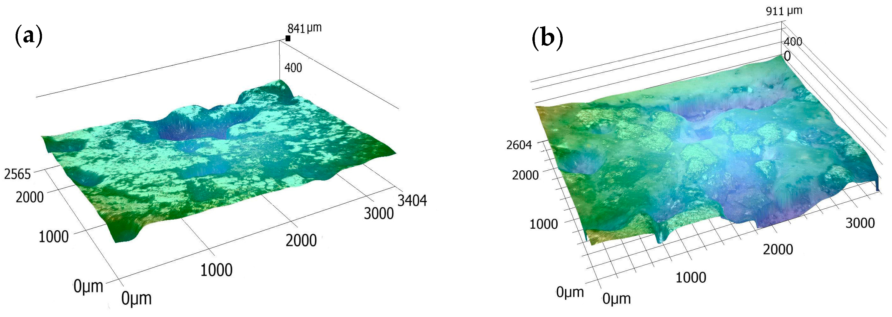
SMS minerals are attached to the seabed with a depth of several thousand meters and must be broken before collection in submarine mining. Due to the peculiarity of the formation mechanism, the interior of SMS is full of pores with a porosity of 20–50% [7,
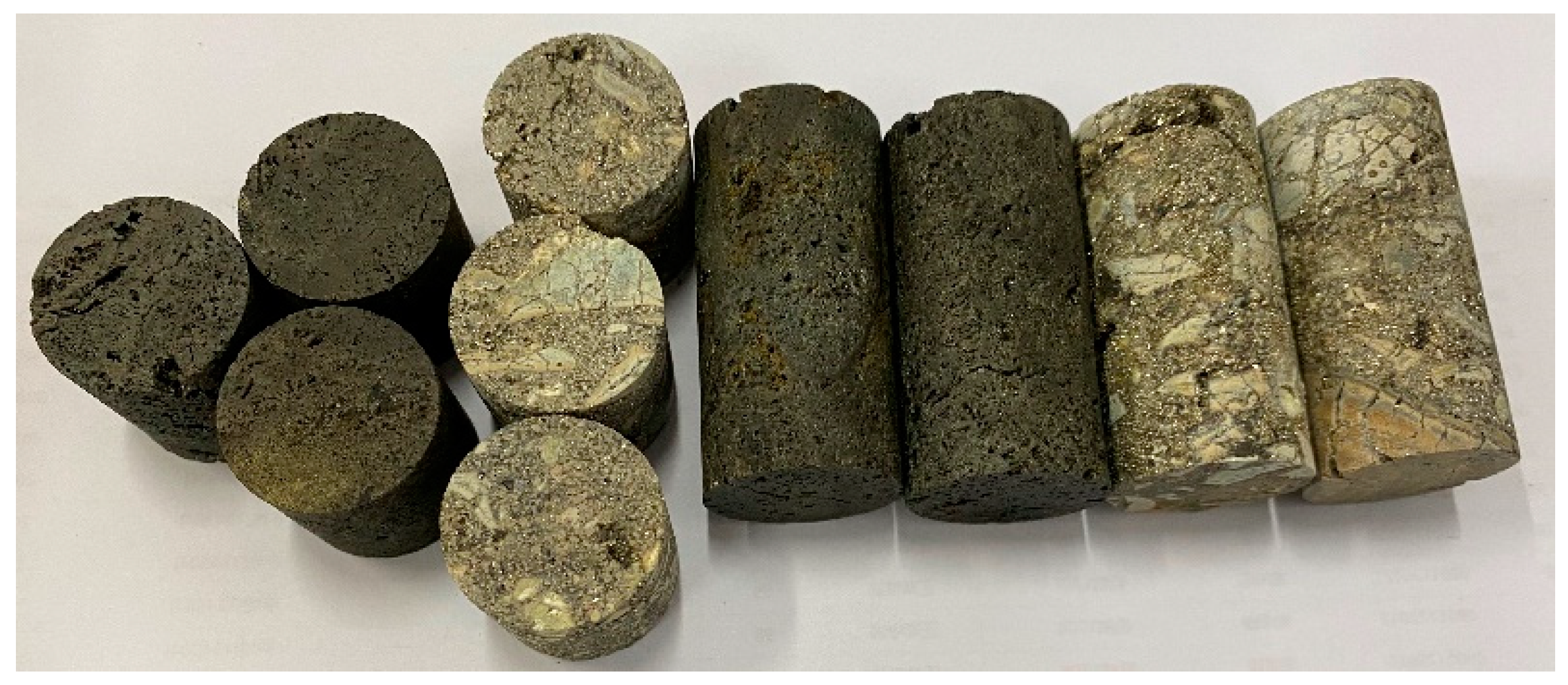
8]. The pores of rock existing in the water depth of several thousand meters are full of seawater, which will be squeezed in the high-speed crushing process, thus affecting the cutting force and the generation of debris. The difference between the study of rock fragmentation in deep-sea mining and land mining is mainly reflected in two aspects. On the one hand, seawater will produce a huge hydrostatic pressure on deep-sea rocks; on the other hand, the pore pressure in the rock will also affect the cutting process. Therefore, it is necessary to study the crushing process of SMS minerals under high ambient pressure so as to provide a basis for the research and design of seabed mining equipment. In this study, the mineralogical study and geotechnical tests of SMS minerals were carried out, and some important mechanical parameters required for numerical analysis were obtained. Although mineralogical investigation is important for an in-depth understanding of SMS, it is not the focus of this study. Then, a two-dimensional simulation model of SMS under hydrostatic pressure is established by using the method of combining discrete element and smooth particle flow. The cutting process of SMS under high hydrostatic pressure is simulated, and the crack evolution, stress distribution, and load characteristics in the crushing process are analyzed. It provides a certain theoretical basis and technical support for deep-sea mining.

2. Mechanical Property Test

2.1. Sample

While studying the fragmentation properties of SMS, we need to have a more comprehensive understanding of their material properties. Therefore, we applied for samples from the China Ocean Sample Repository for material and mechanical property tests and received two pieces of SMS ores. Both samples were collected from the southwest Indian Ocean ridge with a grab bucket, and the sample segments were 30iv-swir-s012tvg01 and 34iv-swir-s035tvg08, respectively.
We used a vhx-5000 ultra-high magnification lens zoom 3D microscope to observe the polished sections of two SMS samples. The 3D microstructure and morphology of the SMS sample are shown in Figure 1. It can be seen that the polished surface of the sample shows many pits of different sizes, which strongly confirms the porous characteristics of SMS. The porosity of the black and white samples is 20.94% and 25.86%, respectively. Generally speaking, porosity is inversely proportional to the stability of minerals. The micro-cracks produced by the pores are easy to expand during the compression process. Then the rock samples become unstable and damaged, affecting the bearing capacity and reducing the strength.
In order to explore the relationship between mechanical properties and mineralogical properties of minerals, the quantitative composition of minerals was determined by XRD. As shown in Table 1, the basic mineral phases in the black sample are pyrite, marcasite, and chalcopyrite. In contrast, the iron in the white sample basically exists in the form of pyrite. Based on the elemental test of SMS minerals in the same mining area [10] and the research results of other scholars [8], we have reason to speculate that other components (including amorphous) are mainly silica.

2.2. Mechanics Test

Due to the limitation of the size, the sample in the geotechnical mechanics test is processed into a non-standard size. The sample in the triaxial compression strength (TCS) test is processed into 25 × 50 mm, and the sample size in the Brazilian splitting test is 25 × 25 mm, as shown in Figure 2. It shows that there are a large number of pores and defects in the sulfide sample so the sample is sealed in a heat-shrinkable tube in the triaxial compression test to prevent hydraulic oil from entering the sample during the test and affecting the determination of mechanical properties. It should be noted that before the triaxial compression test, it is necessary to repair the obvious holes on the sample surface with lime or cement to prevent the high confining pressure oil from penetrating the heat-shrinkable tube and causing the test failure.
The triaxial compressive strength test determines the triaxial compressive strength of rock specimens under different lateral pressures. Equal lateral pressure conditions ( σ 2 = σ 3 ) used in the triaxial compression test are determined according to the engineering needs and rock characteristics. The load acting on the unit area of the specimen is called the compressive strength, which is defined as the ratio of the critical load to the cross-sectional area perpendicular to the load direction. This relationship can be expressed as follows:
R = P A
with the TCS of SMS R, MPa; the failure load P, N; and the cross-section area perpendicular to the loading direction A′, mm2.
In the triaxial compression test, 11 specimens were prepared for both samples, and lateral pressure was set at 2 MPa, 5 MPa, 8 MPa, and 10 MPa, respectively. Because the porosity of the white sample is higher and the internal structure of the mineral is looser, the white sample fails more times in the experiment.
Because the Brazilian splitting test is simple and the results are close to those measured using the direct tensile method, it is used to measure the tensile strength of SMS specimens. The maximum tensile stress acting in the center of the specimen is calculated according to Equation (2).
σ t = 2 P π d t
where σt is the maximum tensile stress in the center of the specimen, MPa; P is peak tensile force at failure, N; and d and t are diameter and thickness of the pressure-bearing disc, mm.
Figure 3 shows the failure modes of the two samples after the TCS test and the Brazilian splitting test, indicating that SMS conforms to the failure characteristics of typical brittle materials. Table 2 illustrates the final mechanical property parameters of the two samples, including the UCS, tensile strength, elastic modulus, internal friction angle, and cohesion.

3. Fluid-Structure Coupling Method

In underwater rock cutting simulation, how to treat the separate phases, solid and fluid, and the coupling between these two has always been one of the key difficulties. Therefore, we established a numerical model of rock drainage effects through DEM-SP coupling. It should be noted that the two methods of DEM and SP have similar algorithms, but the interaction and scope of interaction in the algorithms are different. Among them, the coupling model of pore fluid pressure between particles and rock is transformed into a pore pressure diffusion equation, which is solved by the method based on the smooth particle (SP) technique. The coupling between the two phases is based on the force generated by volume deformation and pressure gradient.

3.1. Rock Model—DEM

The discrete element method can treat the rock mass as a discontinuous discrete medium, in which there may be large displacement, rotation, sliding, and even block separation, so it can truly simulate the discontinuous and large deformation characteristics of the rock mass. Itasca-PFC is widely used in geotechnical engineering, geological engineering, mechanical engineering, and other fields. In PFC, rock material is represented as rigid spherical (3D) or circular (2D) discrete elements (particles) [28]. The interaction between any two particles is realized by the contact constitutive model between particles. The constitutive model is composed of the stiffness model, the slip model, and the bond model, which control the deformation, separation, and movement of particles. The translation and rotation of particles are controlled by the standard equations for rigid body mechanics:
m i u ¨ i = F i
I i ω ˙ i = T i
where Fi and Ti are the sums of force and moment of particle i , respectively, m and I are the mass and moment of inertia, u is the position vector of particle centroid in a fixed coordinate system, ω is the angular velocity. The vectors Fi and Ti are calculated by Formulas (5) and (6).
F i = F i e x t + j = 1 n i c F i j c o n t + F i d a m p + F i p
T i = T i e x t + j = 1 n i c S i j c × F i j c o n t + T i d a m p
where, F e x t and T e x t are external loads, F i j c o n t is the interaction between particle i and adjacent particle, j = 1 , …, n i c , with n i c is the number of neighboring particles in contact with the particles i , Numerical damping load F i d a m p and T i d a m p , S i j c are the vector connecting the centroid of particle i and the contact point of particle j . The contact force F i j c o n t can be decomposed as normal component and tangential component. F i p is the coupling force generated by the fluid pressure gradient on the particle, which will be described in Section 3.2. the numerical damping is defined by Formulas (7) and (8).
F i d a m p = α F i e x t + F i c o n t u ˙ i u ˙ i
T i d a m p = α T i e x t + T i c o n t ω ˙ i ω ˙ i
with α, the numerical damping coefficient.

3.2. Fluid Model—Smooth Particle

Owing to the low permeability of rock-like materials, the contribution of hydrodynamic effects to mechanical rock properties mainly depends on the pressure gradient [29]. In the case of deep-sea excavation with a high cutting speed, the influence of internal fluid speed on the mechanical behavior of rock can be ignored. Furthermore, the thermal effects are negligible relative to the fluid pressure effect. Then, the final pressure diffusion equation is described as follows.
D p D t M ( κ μ p ) = α M D ε V D t
with pore pressure p, Biot modulus M, intrinsic permeability κ, dynamic viscosity of fluid µ, effective stress coefficient α, volumetric strain εV.
Due to the discontinuity of DEM, the continuity Equation (9) cannot be solved directly. Therefore, the pressure diffusion equation is coupled with DEM by applying the interpolation technology based on the smooth particle (SP) method, which weights and accumulates the attributes of each particle around by kernel function. Here we also select Wendland C2, a kernel function with good consistency, a small compact domain, and smoothness, for correction. The calculation method of field quantity A is shown in Formula (10).
A ( u i ) j A j m j W ( r i r j , h ) j m j W ( r i r j , h )
where m is particle mass, W is kernel function, h is smoothing length, with index i for the particle under consideration and index j for the neighboring particles (including particle i).
However, the higher derivative of Formula (9) cannot be calculated directly. Therefore, the diffusion term is discretized by using a method similar to that of Cleary and Monaghan [30] for simulating heat conduction. The diffusion terms can be expressed as
( κ μ p ) = j m j ( κ i + κ j ) ρ i ( μ i + μ j ) ( p i p j ) n i j W ( r i r j , h ) r i r j
According to the pore pressure distribution, the local pressure gradient of the fluid is calculated. Then, the pressure gradient on the particles is added as an interaction force to the external force acting on the particles.
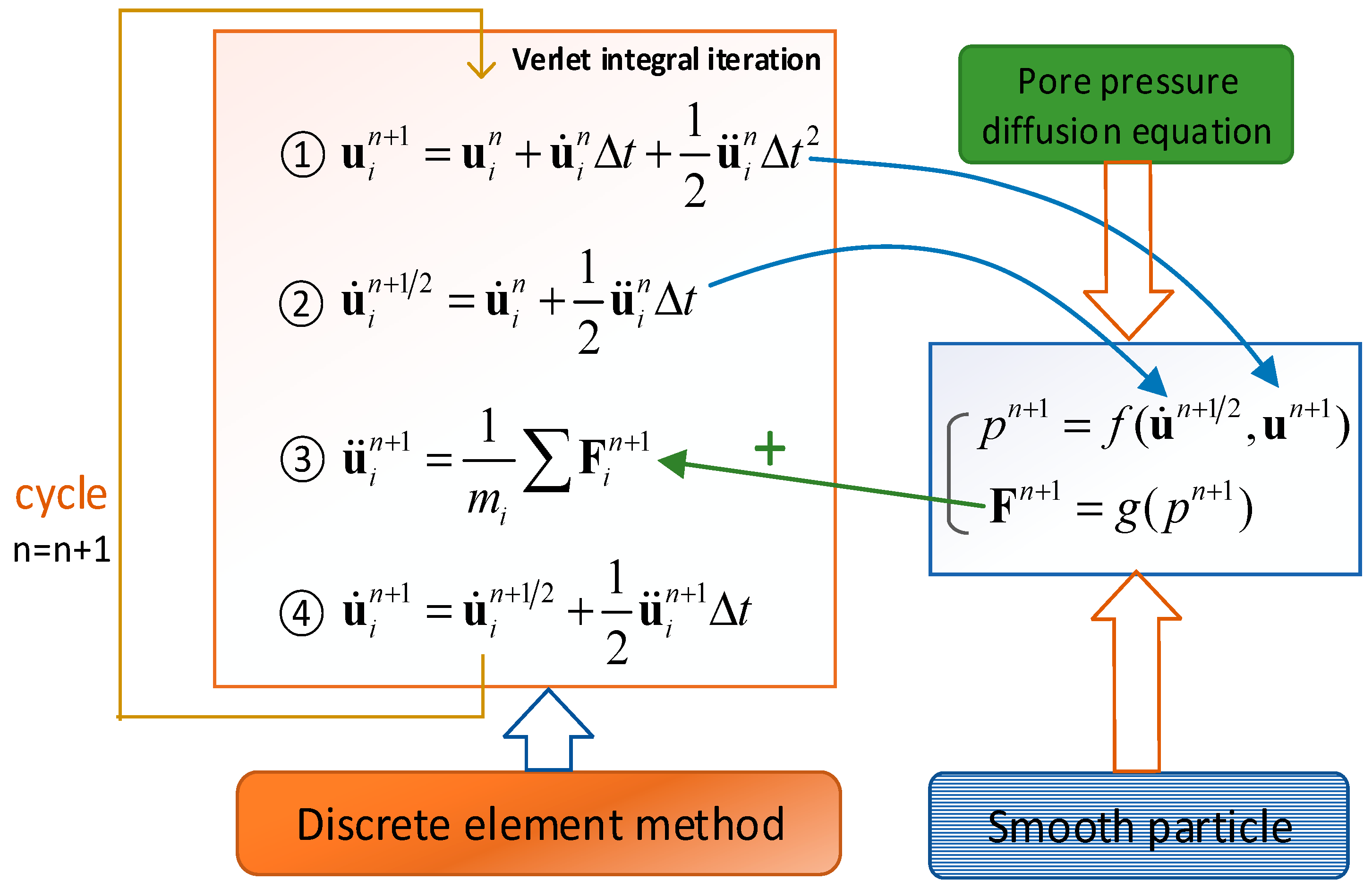
F i = p π r i 2
As illustrated in Figure 4, the coupling force generated by the fluid pressure gradient on the particle builds a bridge between the fluid phase and the discrete phase. The pressure gradient on a particle is added as an interaction force to the sum of forces acting on the particles as Equation (12). Then DEM is advanced half a timestep and the volumetric strain rate is calculated for the fluid based on the intermediate velocities of the DEM particles. It is then used to promote pore pressure diffusion once again. In the whole simulation, the interpolation points of SP coincide with the centroid of DEM particles and move with the movement of DEM particles. In addition, bidirectional coupling is applied at each time step.

3.3. Boundary Identification

In the process of underwater cutting, the water around the mineral boundary flows freely, while the internal liquid is in a restricted flow state due to the restriction between particles. Therefore, the boundary particles in high-pressure fluid should be identified first in numerical simulation. In addition, due to the random fragmentation of rock cuttings and the fact that the internal particles may also become the external boundary, the boundary recognition should be real-time and dynamic. Thus, a method that can deal with disordered particle structure and uneven particle size and mass distribution is needed in the process of boundary recognition. These requirements can be achieved by using the position divergence formula proposed by Muhammad et al. [31].
r = r x x + r y y = 2
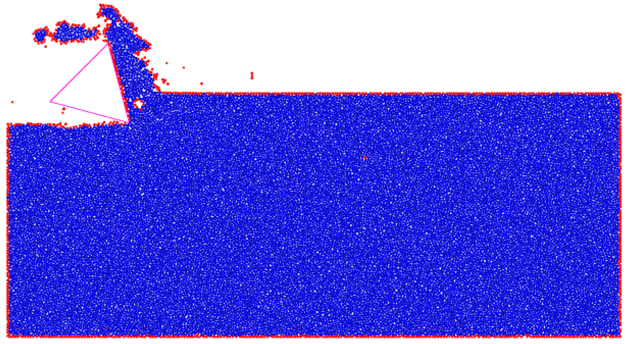
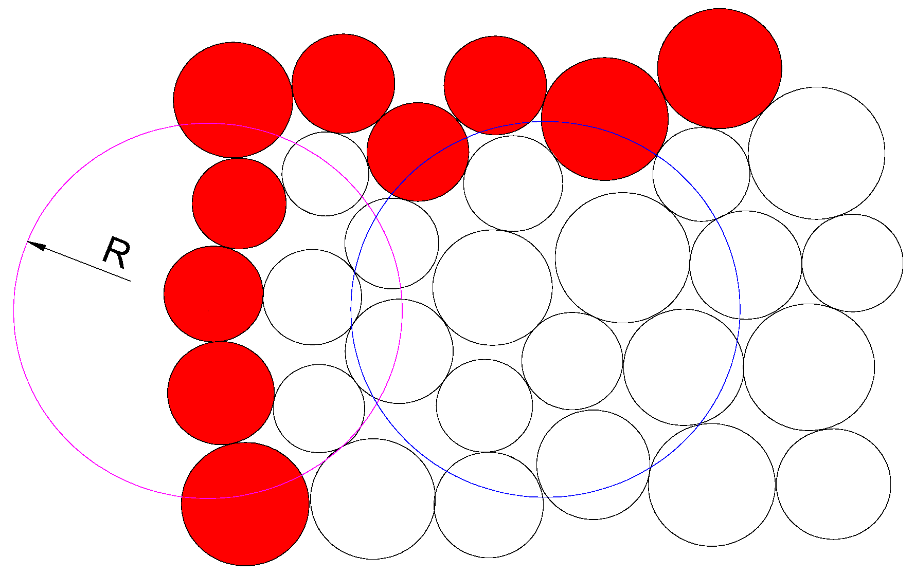
Equation (13) is also applicable to Lucy’s (1977) standard smooth particle method to prevent adjusting position divergence to particle defects at the boundary. As shown in Figure 5, it is assumed that Equation (13) is valid within the blue search radius r. However, if the search range (such as the magenta search circle) is at the boundary, r will be less than 2 due to fewer particles. In this work, particles with r < 1.5 are considered to be boundary particles. In fact, when the search radius is given in the model, the average number N of adjacent particles of each particle within the search radius is constant. Specifically, particles with fewer than (1.5/2) × N particles in the search domain are judged as boundary particles. Eventually, all boundary particles are identified, and their pressures are fixed to the target value. Generally speaking, a larger search radius leads to more accurate particle judgment, but the computational overhead also increases correspondingly. Therefore, it is necessary to balance the accuracy and computational expense of the research.

3.4. Implementation Method

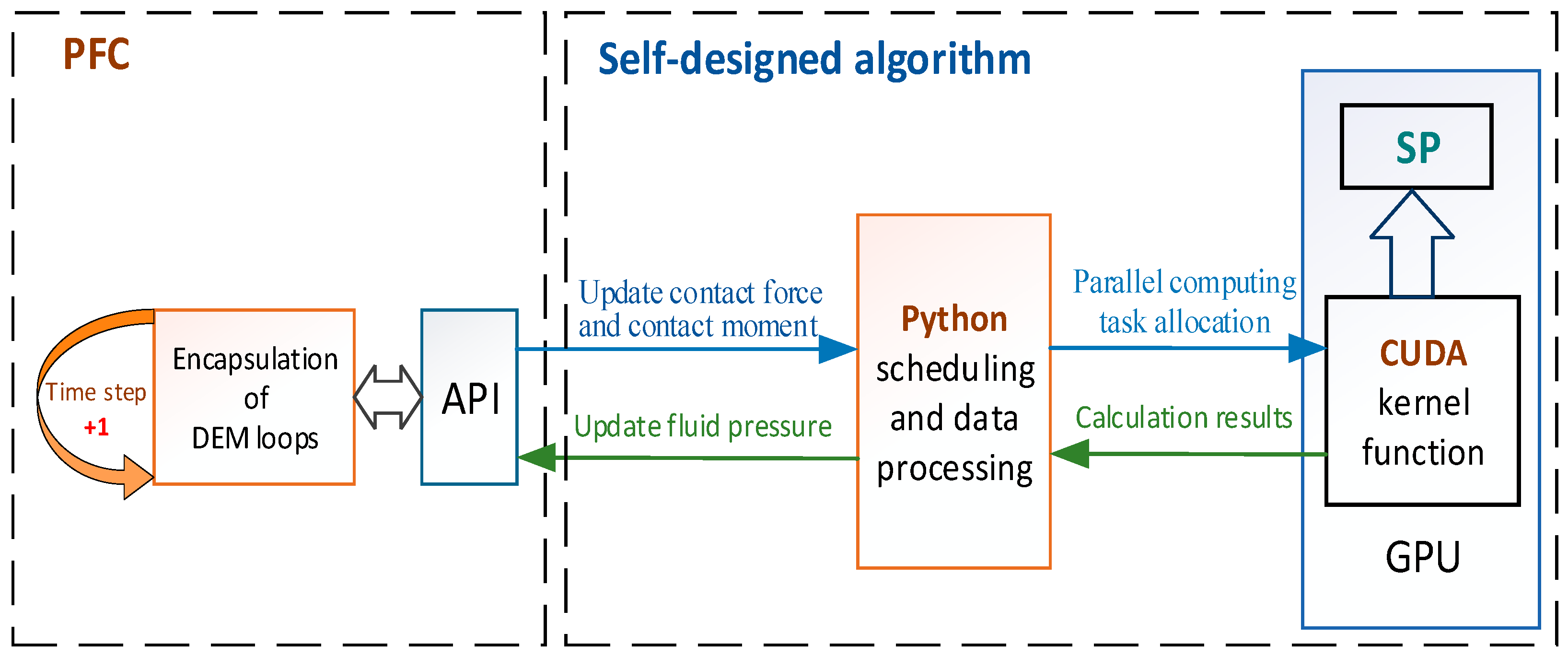
PFC provides the Python environment and the interface API between these two. Figure 6 shows the DEM-SP model implementation architecture. Python first calls the specific API of PFC software to obtain the velocity vector and position vector of discrete particles in PFC at n + 1/2 steps. After Python preprocessing, it is submitted to the CUDA computing core on the GPU for parallel computing. By substituting the data into the fluid pressure diffusion equation, the fluid pressure of the particle located and the coupling force generated are calculated. Then, the data is transferred back to PFC through a specific API, and the external force is applied to the particles to realize the coupling of the discrete phase and fluid phase. After that, PFC updates step n + 1, and iteration was achieved according to the above process.
The DEM part of the simulation is written in the fish language provided by PFC. In contrast, the fluid part is programmed with the CUDA module provided by the Numba library and accelerated through real-time compilation. Before calling the Python program every time, the kernel function written by CUDA was compiled, and then GPU was called to accelerate the above program calculation. The Python program is called by PFC software in the form of a plug-in. Once the Python file is called and run, Python will read the parameters provided by PFC and perform some steps, such as parameter initialization, variable initialization, GPU initialization, etc. Then the CUDA kernel function, data exchange, and coordination functions of the GPU are defined, and finally, the iterative function is inserted into the PFC operation step through a callback. Each iteration of PFC will automatically call the CPU data exchange and coordination functions defined by Python and GPU calculation functions for hydrodynamics calculation so as to realize coupling calculation. Since two-dimensional cutting is more convenient for analyzing the cutting mechanism and stress from the meso point of view, the algorithms and simulations are set up in 2D.

4. Material Calibration and Model Establishment

4.1. Material Calibration

The difference in mineral formation environments and conditions result in significant differences in mechanical parameters measured by different types of samples in different regions. As described in Section 1, we obtained the basic mechanical parameters of two SMS samples. However, the macro mechanical parameters of ore samples cannot be directly used in simulation. They should be calibrated repeatedly by biaxial compression, uniaxial compression, and other simulation tests to determine the appropriate meso parameters so that the numerical model has the same macro performance as the real experiment.
For SMS, its macroscopic characteristics are not only able to bear the action of tension and compression but can also resist bending and torsion. Meanwhile, based on the consideration of nonlinear forces in ore, we chose the parallel bond model and linear contact model as the contact models between particles and between particles and tools. In the calibration, particles obey a uniform size distribution with a radius of 0.5–0.75 mm. Practice has proved that it is easy to simply meet the requirements of compressive strength or tensile strength. However, no matter how to adjust the combination of normal and tangential bond strength, it cannot meet the ratio of tensile strength to compressive strength. This is because the actual rock is usually composed of particles with significantly different stiffness. Different particles can coordinate the deformation in the deformation process while using uniform, same-bonding parameters and stiffness parameters cannot reflect this phenomenon. Therefore, a mixed bond parameters model was applied in parameter calibration. Soft particles account for 40% of the total, and their tangential and normal strengths are 5% of the hard particles. The micromechanical parameters of SMS ore calibrated by multiple numerical simulation tests are shown in Table 3, and the corresponding macro parameter error is less than 10%.

4.2. Model Establishment

Deep sea mining is a high-speed cutting process with a large cutting depth. As shown in Figure 7, according to the method described in Section 3, a two-dimensional model of rock breaking with a single cutter is established by using PFC2D software. A linear cutting simulation was carried out on a block with a size of 300 mm × 120 mm and a total number of 24,300 particles, and the particles at the right end and bottom of the ore body model are fixed. In this model, the cutter is modeled as a rigid body by using the wall element, and the cutter breaks the ore at a constant speed v. The cutter is placed at an inclination of 45° with a tip angle of 60° and a cutting depth of 15 mm. In the 2D simulation, the cutting process is carried out with a pressure of 0 MPa, 10 MPa, 20 MPa, and 30 MPa, respectively, according to different mineral occurrence depths.
We build the model according to the framework shown in Figure 6 and set the liquid phase parameters after coupling with PFC2D through Python and a CUDA self-made algorithm, as shown in Table 3. The dynamic viscosity of water is 0.001 pa·s, and the permeability of SMS rock is set at 1 × 10⁻¹⁵. The real-time pore liquid pressure in the numerical calculation process is transmitted to PFC2D through API to promote iterative calculation. During the simulation, the model status was saved every 0.005 s, and the contact force of particles, the information of particles, cracks, and chips were also recorded.

5. Intact Coupling Cutting Process

To investigate the cutting mechanism of deep-sea minerals, several intact simulations of the coupled cutting process were performed. According to the method described in Section 3.3, the radius of the boundary recognition domain is set to 2.8 mm. Consequently, particles with fewer than 13 particles within the research domain are considered to be fully surrounded by hydrostatic pressure, and the coupling force of these particles is zero. It should be noted that in order to avoid large deviations in the number of particles in each interpolation domain and reduce the possibility of particles being misjudged, the ratio of maximum radius to the minimum radius of particles should not be too large. Figure 8 shows the results of boundary recognition, in which the red circles represent the boundary particles recognized by the algorithm. Although several misjudged particles were found in the model, the overall effect is good.
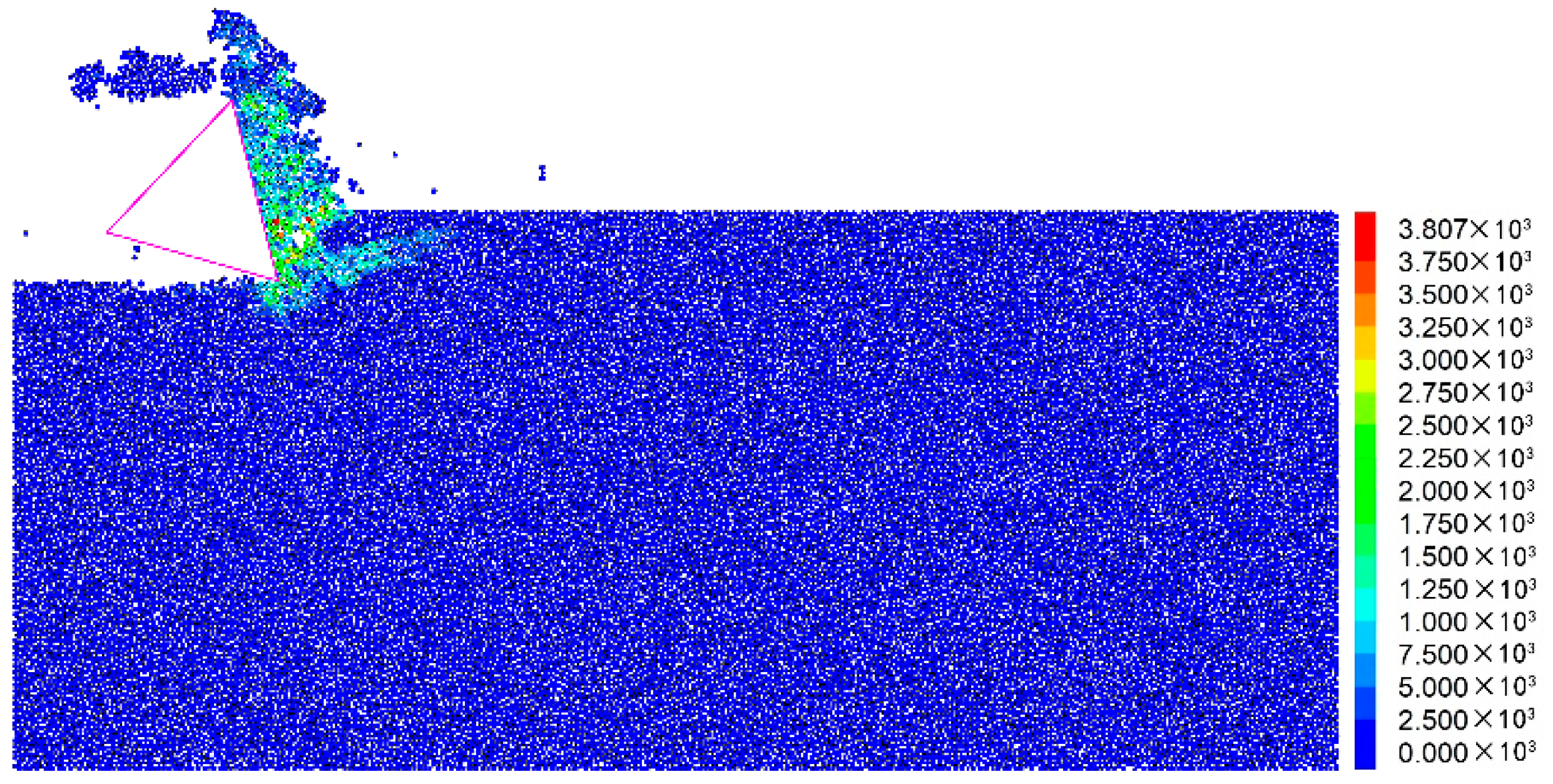
The strong impact of the cutter forces the rock particles to disconnect and move away, and the separate particles represent the rock fragments that have been cut away. In the cutting process, the pore fluid pressure is applied to the particle center by PFC2D in the form of an external force, which is constantly updated by calculating the fluid pressure diffusion equation. According to the theory introduced in Section 3.2, the external force is formed by the pressure diffusion caused by the increase or decrease of the pore volume. Consequently, the external force exerted on particles is mainly concentrated at the front and bottom of the contact surface, while it is zero on the particles at other positions (Figure 9). Due to the relative motion between the parallel bonded particles, the contact force or moment along the relative direction will be generated. The bond will break, and microcracks form in the case where the contact force exceeds the bond strength. The particles separate and move under the combined action of the strong impact of the cutter and the fluid pressure. As the cutter moves forward, the pore pressure is also updated iteratively.
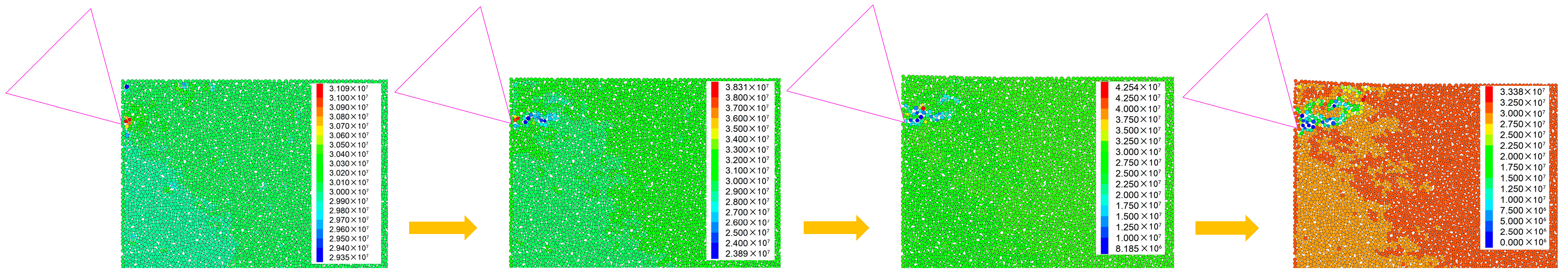
More interestingly, with the use of the DEM-SP coupling method, it is possible to investigate effects that are difficult to measure, such as the pore pressure distribution. Figure 10 shows the pore fluid pressure diffusion process in local rock samples around the tip. When the tip of the cutter wedges into the rock, local pore compression occurs due to particle extrusion, resulting in an increase in local fluid pressure, as shown in Figure 10. With the gradual advancement of the cutting tool, the bond between particles is destroyed, and cracks appear, which leads to local pore expansion and further leads to the reduction of pore pressure. The low pore pressure area in front of the tool tip indicates that the rapid deformations applied to the rock might result in cavitation of the pore fluid.
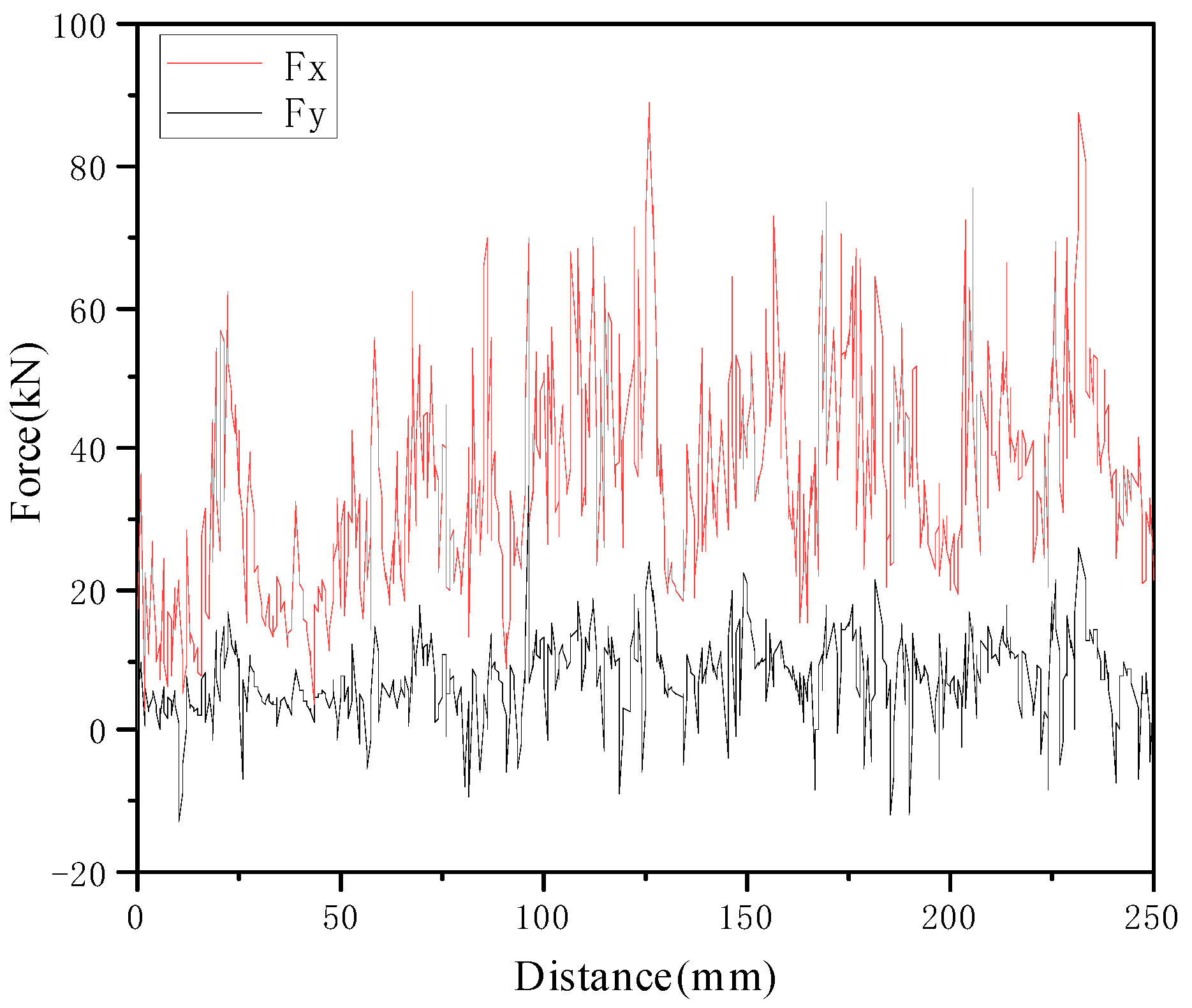
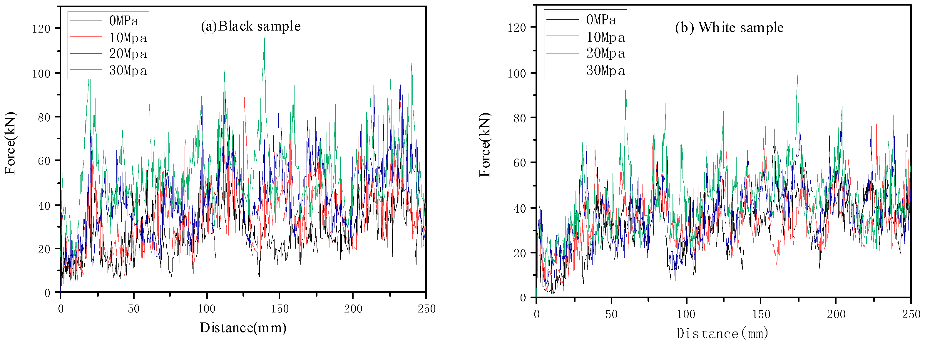
Figure 11 shows a variation history of the x and y components of tool force in cutting the black sample, where positive Fx represents the force in the opposite direction of tool advance, and positive Fy represents the tool being pulled into the rock. Since the model is two-dimensional, the force refers to the force on the tool per unit thickness. The rock-cutting process is a typical cycle of elastic deformation, crack initiation, propagation, and failure. Accordingly, the cutting force oscillates as saw-teeth in the cutting process. The upward stage of the curve represents that the tool resists the adhesion between particles. The downward stage represents that the pick penetrates the rock to form microcracks, which are combined into macro cracks to form rock cuttings. As the cutter advances, the cutting force fluctuates with the formation of chips. Due to the randomness of crack propagation and chips, the peak value and period of cutting force in each cycle are not consistent. In the whole cutting process, the main cutting force Fx along the tool speed direction is dominant, which is also the main source of energy consumption. Thus, the subsequent detailed analysis related to the cutting force is only completed for the main cutting force Fx.

6. Results and Analysis

6.1. Crack Evolution

In order to further analyze the influence of fluid pressure on fragmentation characteristics of the SMS specimen from the mesoscopic point of view, the cumulative changes of microcracks were recorded by the program. As the simulation starts, the tool gradually contacts the sample, and then an initial crack is generated beneath the pick tip, which is called crack initiation. As the tool continues to advance, the crack propagates further until the fragment spalls. In PFC2D, the microcracks can be divided into tensile cracks and shear cracks according to fracture forms, which are represented by red and green segments, respectively, in this work. Figure 12 shows the distribution of cracks with displacement at the end of the simulation of SMS samples under different ambient pressures. Cutting rock under different fluid pressures is mechanically a comprehensive failure mode, accompanied by tensile and shear cracks. Although there is no obvious signal that tensile cracks or shear cracks are dominant, we can observe that the crack propagation is deeper under low confining pressure. At the same time, the internal damage of the model is more likely to occur under higher pressure, such as 20 MPa and 30 MPa. Regardless of the pore pressure, some chips collide with the high-speed moving tool in the simulation, accompanied by secondary breakage.
The cumulative number history of micro-cracks under different confining pressures was further recorded by the program. As illustrated in Figure 13, the cumulative number of cracks under no confining pressure is similar to a step-by-step change. Thus, the fracture process can be divided into two types of stages: one is the crack accumulation and propagation stage, which is the main cutting process. The other stage is when the chips fall off, the tool pushes the chip forward, accompanied by a certain degree of secondary crushing, and the number of cracks is less in this stage. However, the alternating frequency of the two stages accelerates, and the cumulative crack growth rate is obviously accelerated with the increase in pressure. Figure 14 shows the relationship between the ratio of tensile crack number to shear crack number and hydrostatic pressure. The ratio has no obvious regularity with the increase of pressure, which is different from the usual simulation in which pressure is favorable for shear failure. This is mainly determined by the shear strength and tensile strength between particles in the parameter calibration. Grima et al. [14] interpret that the cutting process under high-pressure changes into an apparent ductile (cataclastic) mode and the failure of the rock will be predominately shear. When ductile behavior prevails, the crack formation is mostly along shear planes, and more force will be required to create a chip.

6.2. Load Characteristics

The horizontal cutting force Fx with respect to cutting distance for different rock models is shown in Figure 15. We can see that the overall horizontal cutting force is positively correlated with the ambient pressure, which is true for both black and white sample models. Moreover, pressure seems to have a greater influence on the black model. It is worth noting that for the two samples, the tool force will not drop to 0 when it drops from the peak value. This is due to the high-speed movement of the cutter, which causes the cutter to continuously contact a large amount of debris and cause secondary crushing.
Figure 16 indicates the relationship between the ambient pressure and the average cutting force for the black and white rock models. The average force for both the two rock models increases with the increases in ambient pressure. For instance, the average cutting force of the black sample under the pressure of 10 MPa, 20 Mpa, and 30 MPa is 30.8%, 55.2%, and 97.8% higher than those in the atmosphere, respectively. The average peak cutting force also increased from 57.6 MPa to 76 MPa, 85.2 MPa, and 102 MPa, respectively. While the average cutting force and the peak cutting force of the white sample increase with ambient pressure at a lower speed than those of the black sample. Although the strength of the black sample is about 1.5 times that of the white sample, the force changes of the two different materials do not show significant differences. In other words, there is no evidence that the difference in mechanical properties plays a dominant role in high-pressure and high-speed rock cutting. Under the combined action of high pressure and high speed, serious secondary crushing occurs in the cutting process. In contrast, the influence of rock strength on cutting force is relatively weak. As the average peak cutting force is significantly greater than the average cutting force, it is a more reasonable parameter for evaluating the working state of the pick and designing the excavation equipment. The fitting curve of the black specimens was y = 1.43x + 58.7, R2 = 0.985. The fitting curve of the white specimens was y = 0.72x + 62.99, R2 = 0.984. The correlation coefficient R2 of the two models was greater than 0.98, which shows a good correlation between the ambient pressure and average peak cutting force for the two SMS specimens.

6.3. Fragment Morphology

Figure 17 shows the shape of debris at the end of the simulation under different hydrostatic pressure, where different color blocks represent chips generated in the cutting process. It can be seen that chips of different sizes are dispersed above the model, and the randomness of size is very strong, showing strong brittleness in atmospheric conditions. In contrast, in high-pressure conditions, the chip is finer and uniform in general. This is because the increase of confining pressure leads to more severe fragmentation in the crush zone and more difficult crack propagation, thus resulting in finer fragments. According to the research of Grima [14], lumps with the appearance of clay rather than chips are formed in the high-pressure cutting process, and a more ductile process will occur. This is consistent with the chip transformation shown in Figure 17, which verifies the correctness of the simulation in this study. We can also observe that the hydrostatic pressure also has a significant effect on the cutting surface of the model. Since the high pressure inhibits the crack growth, a finer cutting surface is generated, and the size of the crushed zone decreases. In atmospheric conditions, chips are scattered over the model due to the instantaneous breaking of the bonds, while with the increase of the pressure, the particle flow property of debris is stronger.
We also make statistics on the volume of fragments generated in the cutting process (it is actually the area in 2D), in which the volume of each fragment is the sum of the volumes of all particles in the fragment. The statistical data under different pressures is shown in Figure 18. As depicted, the chip size distribution of the two samples with different pressures is similar, and the small size accounts for the majority. Meanwhile, the variation trend of chip size produced by the two samples is basically the same, and there is more small debris and less large debris with the increase of pressure. In other words, the fluid pressure will make the generated debris more uniform, which is consistent with the chip morphology diagram in Figure 17. The existence of fluid pressure will inhibit the extension of cracks and make the size of debris smaller.

6.4. Specific Energy

Specific energy (SE)is an important and valid parameter to evaluate cutting efficiency, and it is widely used to evaluate the performance of mining and excavation machinery. SE is calculated by:
S E = F R L V
where FR refers to the average horizontal cutting force, L is the cutting distance, and V denotes the total volume of chips. A large amount of powder or fine particles is produced during cutting, but some rocks are still relatively complete. Note that a large amount of powder or fine particles is produced in the cutting process, so it is inaccurate to calculate the volume directly by summing the volumes of all fragments. In fact, the calculation error can be reduced by subtracting the remaining volume from the original volume of the sample model.
Figure 19 shows the relationships between ambient pressure and specific energy for different rocks. For each rock sample, specific energy is positively correlated with the pressure. Moreover, the growth rate of specific energy of black samples with higher strength is obviously higher than that of white samples. This is due to a higher cutting force and a lower total amount of chips with the increase in pressure. Moreover, the slope of the “SE vs. ambient pressure” curve of the black sample is bigger than that of the white sample. This means that the cutting efficiency of black rocks with high strength is more sensitive to ambient pressure than that of white rocks with lower strength.

7. Conclusions

The purpose of this work is to study the effect of high hydrostatic confining pressure on the cutting performance of two SMS seabed minerals. The analysis results draw the following conclusions:
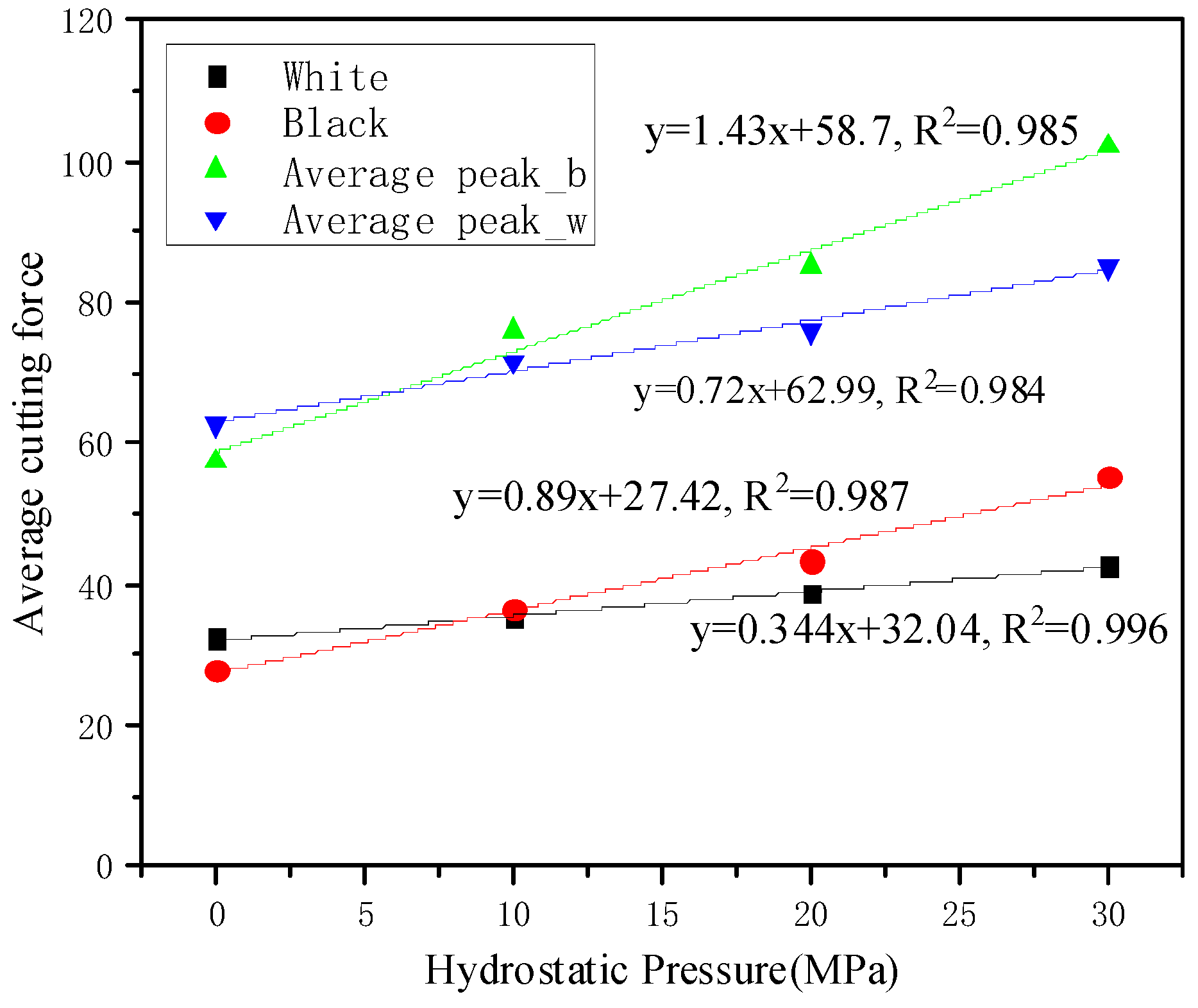
(1) The cutting force is significantly improved with the combination of high cutting speed and high pressure. Furthermore, the cutting forces increase with increasing ambient pressure.
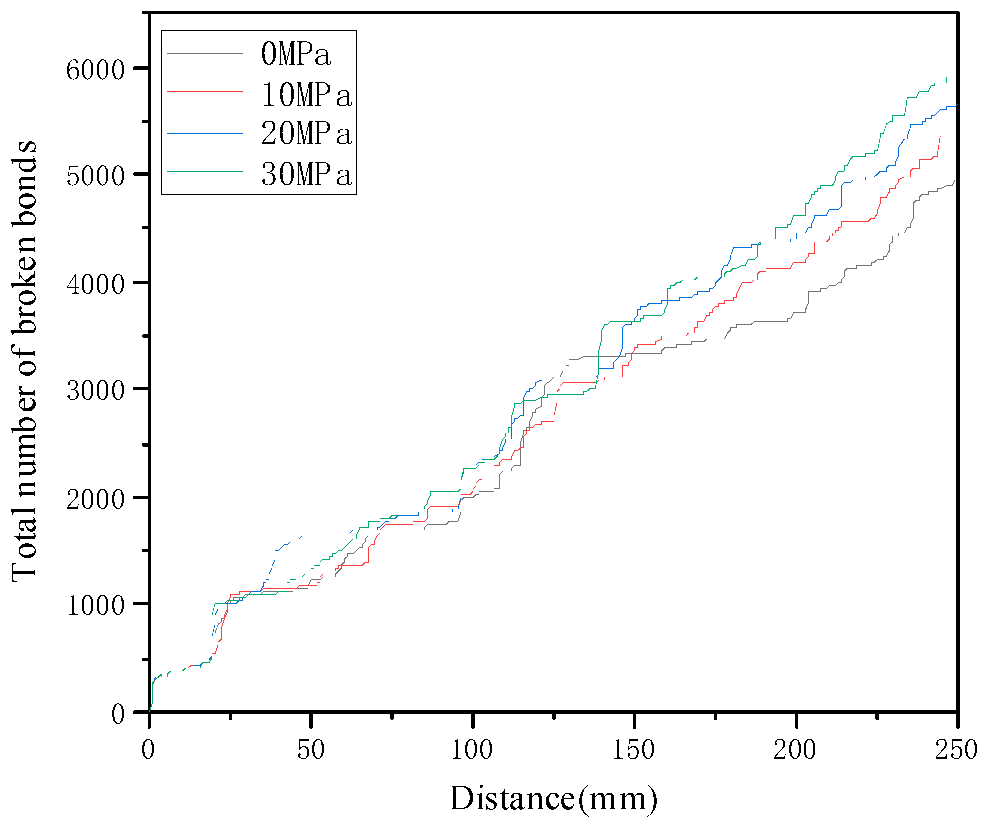
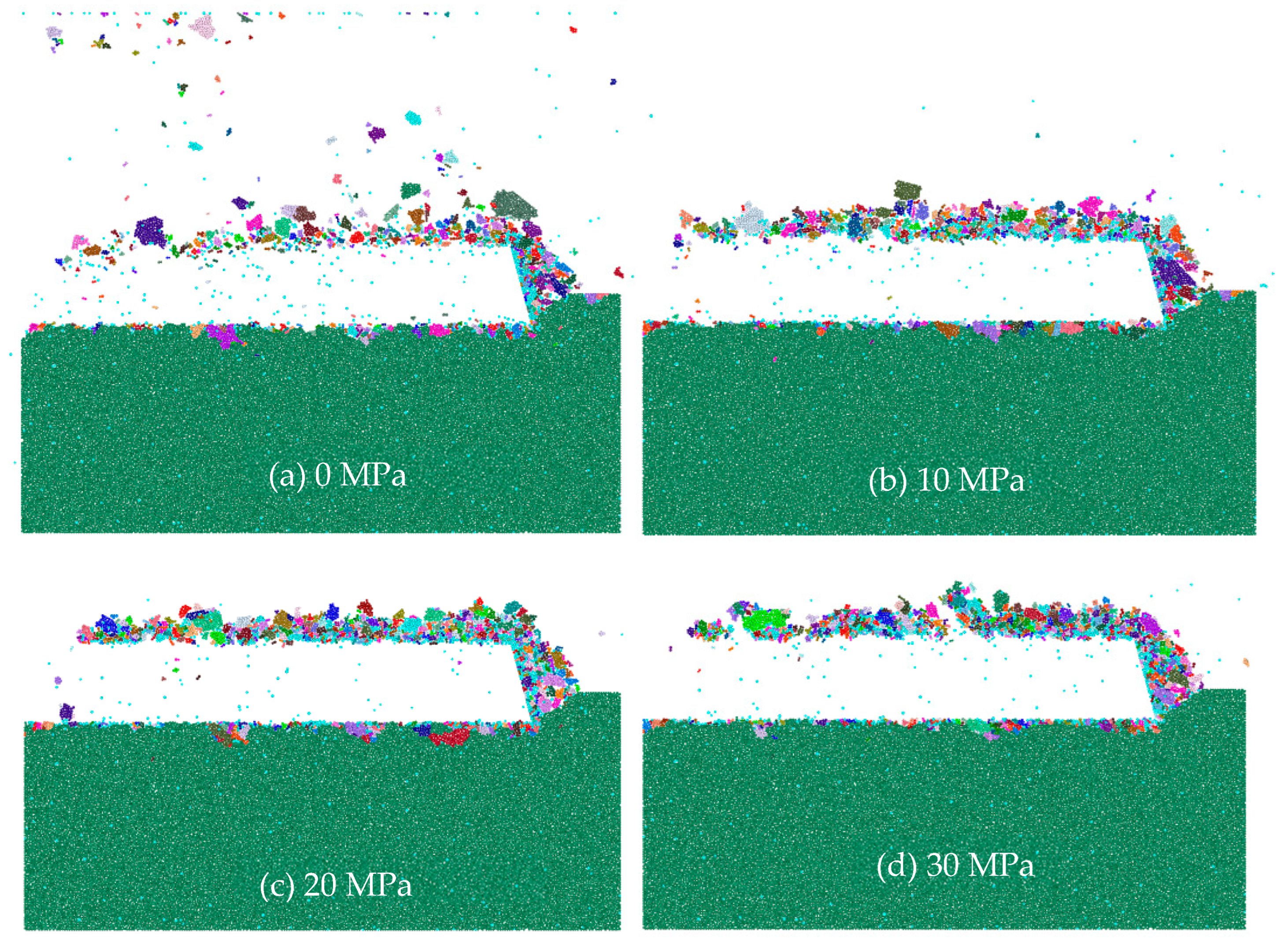
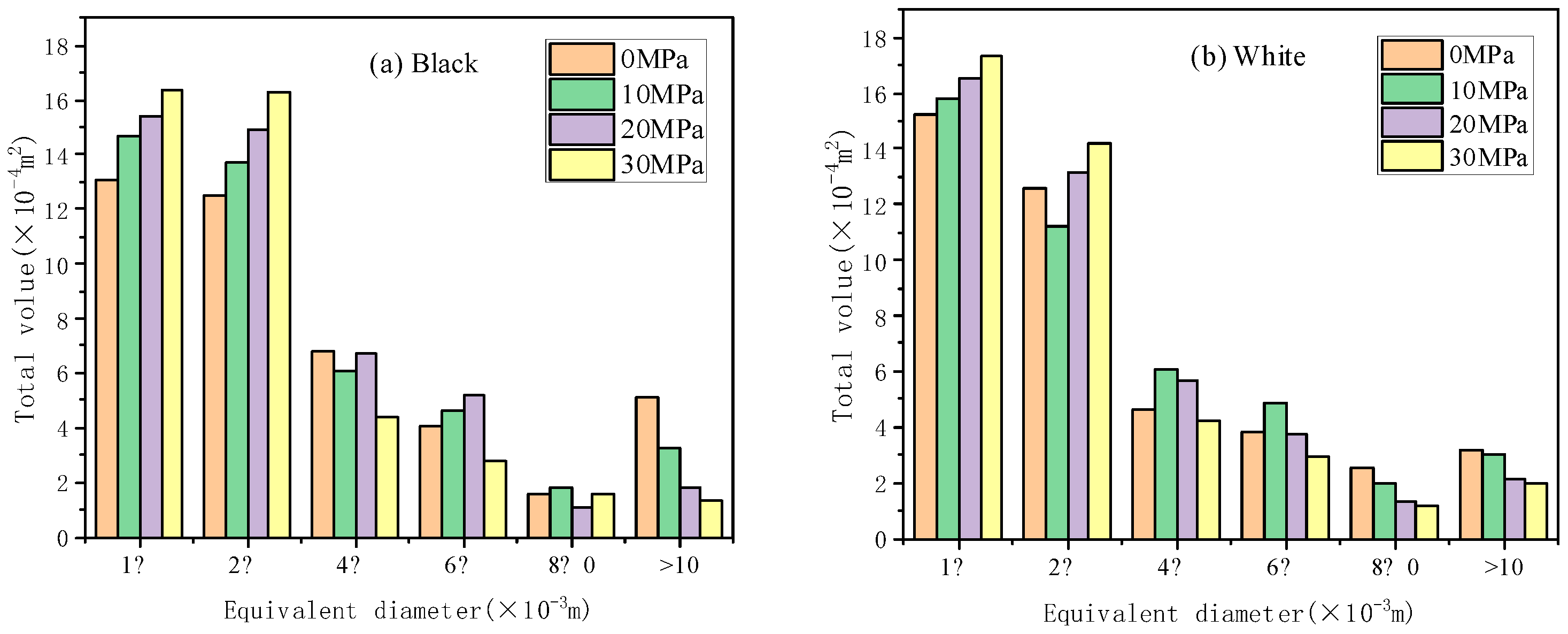
(2) The increase in ambient pressure leads to the variation of chip morphology. With the increase of pressure, fragmentation in the crush zone becomes more severe, and crack propagation is more difficult. For these reasons, the fragments are finer and more uniform, and the cutting surface is flatter.
(3) Compared with the white sample, the cutting force of the black sample with higher strength increases faster with the pressure. At the same time, the specific energy of the black sample is more sensitive to the ambient pressure than that of white rocks with lower strength.
The combination of DEM and SP provides an effective method for the analysis of underwater fluid-solid coupling cutting processes, especially a valuable method for the interaction between materials and tools under hydrostatic pressure. The study of rock fragmentation mechanisms provides important information for the exploitation of SMS. It should be noted that only the influence of pore pressure is considered in the discussion, and the influence of fluid viscous resistance on the trajectory of debris is not considered. In addition, geotechnical characteristics may also have a strong impact on seabed excavation tools. For example, the silica content in seabed minerals can have a strong negative impact on the wear resistance of mining tools. Therefore, in future deep-sea excavation research, a more in-depth and large-scale geotechnical investigation is also necessary.

Author Contributions

The paper emerged from the long-term cooperation of the authors. Conceptualization, Y.L. and H.D.; methodology, H.D.; test and analysis, H.D. and H.L.; writing—original draft preparation, H.D.; writing—review and editing, Y.L. and H.L. All authors have read and agreed to the published version of the manuscript.

Funding

This research was supported by the National Key Research and Development Program of China, grant number 2021YFC2801701-02 and Major Science and Technology Projects of Hunan Province, China, grant number 2020GK1022.

Institutional Review Board Statement

Not applicable.

Informed Consent Statement

Not applicable.

Conflicts of Interest

The authors declare that they have no known competing financial interests or personal relationships that could have appeared to influence the work reported in this paper.

References

  1. Miller, K.A.; Thompson, K.F. An overview of seabed mining including the current state of development, environmental impacts, and knowledge gaps. Front. Mar. Sci. 2018, 4, 418. [Google Scholar] [CrossRef]
  2. Levin, L.A.; Amon, D.J. Challenges to the sustainability of deep-seabed mining. Nat. Sustain. 2020, 3, 784–794. [Google Scholar] [CrossRef]
  3. Leng, D.X.; Shao, S. A brief review of recent progress on deep sea mining vehicle. Ocean Eng. 2021, 228, 108565. [Google Scholar] [CrossRef]
  4. Kato, Y.; Fujinaga, K. Deep-Sea Mud in the Pacific Ocean as a Potential Resource for Rare-Earth Elements. Nat. Geosci. 2011, 4, 535–539. [Google Scholar] [CrossRef]
  5. Boschen, R.E.; Rowden, A.A. Mining of deep-sea seafloor massive sulfides: A review of the deposits, their benthic communities, impacts from mining, regulatory framework and management strategies. Ocean Coast. Manag. 2013, 84, 54–67. [Google Scholar] [CrossRef]
  6. Interridge. InterRidge Vents Database Ver.3.4. Available online: https://vents-data.interridge.org (accessed on 15 July 2022).
  7. Yamazaki, T.; Park, S.H. Relationships between geotechnical engineering properties and assay of seafloor massive sulfides. In Proceedings of the 13th International Offshore and Polar Engineering Conference, Honolulu, HI, USA, 25–30 May 2003. [Google Scholar]
  8. Spagnoli, G.; Jahn, A. First results regarding the influence of mineralogy on the mechanical properties of seafloor massive sulfide samples. Eng. Geol. 2016, 214, 127–135. [Google Scholar] [CrossRef]
  9. Hu, J.H.; Liu, S.J. Deformation characteristics and constitutive model of seafloor massive sulfides. J. Cent. South Univ. 2017, 24, 1986–1991. [Google Scholar] [CrossRef]
  10. Dai, Y.; Ma, F.Y. Mechanical tests and numerical simulations for mining seafloor massive sulfides. J. Marine Sci. Eng. 2019, 7, 252. [Google Scholar] [CrossRef]
  11. Hunter, R.J. Investigation of the Application of Mechanical Mining of Ocean Floor Polymetallic Sulphide Deposits. Master’s Thesis, University of British Columbia, Vancouver, BC, Canada, 2007. [Google Scholar]
  12. Yutaro, S.; Jizhao, L. First successful mining of submarine hydrothermal deposits in the world. Constr. Project. 2020, 72, 83–87. [Google Scholar]
  13. JOGMEC Conducts World’s First Successful Excavation of Cobalt-Rich Seabed in the Deep Ocean. Available online: http://tokiox.com/wp/ogmec-conducts-successful-excavation-of-cobalt-rich/?lang=en (accessed on 15 July 2022).
  14. Kaitkay, P.; Lei, S. Experimental study of rock cutting under external hydrostatic pressure. J. Mater. Process. Tech. 2005, 159, 206–213. [Google Scholar] [CrossRef]
  15. Grima, M.A.; Miedema, S.A. Effect of high hyperbaric pressure on rock cutting process. Eng. Geol. 2015, 196, 24–36. [Google Scholar] [CrossRef]
  16. Detournay, E.; Atkinson, C. Influence of pore pressure on the drilling response in low-permeability shear-dilatant rocks. Int. J. Rock Mech. Min. 2000, 37, 1091–1101. [Google Scholar] [CrossRef]
  17. Li, X.F.; Wang, S.B. Investigation on the influence mechanism of rock brittleness on rock fragmentation and cutting performance by discrete element method. Measurement. 2018, 113, 120–130. [Google Scholar]
  18. Xue, Y.D.; Zhou, J. Rock fragmentation induced by a TBM disc-cutter considering the effects of joints: A numerical simulation by DEM. Comput. Geotech. 2021, 136, 104230. [Google Scholar] [CrossRef]
  19. Shimizu, H.; Murata, S. The distinct element analysis for hydraulic fracturing in hard rock considering fluid viscosity and particle size distribution. Int. J. Rock Mech. Min. 2011, 48, 712–727. [Google Scholar] [CrossRef]
  20. Zeng, W.; Yang, S.Q. Numerical investigation on permeability evolution behavior of rock by an improved flow-coupling algorithm in particle flow code. J. Cent. South Univ. 2018, 25, 1367–1385. [Google Scholar] [CrossRef]
  21. Zhang, Y.L.; Shao, J.F. An improved hydromechanical model for particle flow simulation of fractures in fluid-saturated rocks. Int. J. Rock Mech. Min. 2021, 147, 104870. [Google Scholar] [CrossRef]
  22. Lei, S.T.; Kaitkay, P. Distinct element modeling of rock cutting under hydrostatic pressure. Key Eng. Mat. 2003, 250, 110–117. [Google Scholar]
  23. Rizo, M.A.J. Considerations for Discrete Element Modeling of Rock Cutting. Ph.D. Thesis, University of Pittsburgh, Pittsburgh, PA, USA, 2013. [Google Scholar]
  24. Tropin, N.; Manakov, V. Implementation of boundary conditions in discrete element modeling of rock cutting under pressure. Appl. Mech. Mat. 2014, 598, 114–118. [Google Scholar]
  25. Lv, Y.; Li, H. Bonded-cluster simulation of rock-cutting using PFC2D. Clust. Comput. 2017, 20, 1289–1301. [Google Scholar]
  26. Helmons, R.L.J.; Miedema, S.A. Simulating hydro mechanical effects in rock deformation by combination of the discrete element method and the smoothed particle method. Int. J. Rock Mech. Min. Sci. 2016, 86, 224–234. [Google Scholar] [CrossRef]
  27. Helmons, R.L.J.; Miedema, S.A. Modeling fluid pressure effects when cutting saturated rock. Eng. Geol. 2016, 211, 50–60. [Google Scholar] [CrossRef]
  28. Potyondy, D.O. The bonded-particle model as a tool for rock mechanics research and application: Current trends and future directions. Geosys. Eng. 2015, 18, 1–28. [Google Scholar] [CrossRef]
  29. Helmons, R.L.J. Excavation of Hard Deposits and Rocks on the Cutting of Saturated Rock. Ph.D Thesis, Delft University of Technology, Delft, The Netherlands, 2017. [Google Scholar]
  30. Cleary, P.W.; Monaghan, J.J. Conduction modelling using smoothed particle hydrodynamics. J. Comput. Phys. 1999, 148, 227–264. [Google Scholar] [CrossRef]
  31. Muhammad, N.; Rogers, B.D. Understanding the behaviour of pulsed laser dry and wet micromachining processes by multi-phase smoothed particle hydrodynamics (SPH) modelling. J. Phys. D Appl. Phys. 2013, 46, 95101. [Google Scholar] [CrossRef]
Figure 1. Micrograph of the polished surface in three dimensions:(a) black sample, (b)white sample.
Jmse 10 01306 g001
Figure 2. Processed test samples.
Jmse 10 01306 g002
Figure 3. The failure samples in: (a) TCS test; (b) Brazilian splitting test.
Jmse 10 01306 g003
Figure 4. Flowchart of the coupling in DEM-SP.
Jmse 10 01306 g004
Figure 5. Boundary recognition.
Jmse 10 01306 g005
Figure 6. DEM-SP model implementation architecture.
Jmse 10 01306 g006
Figure 7. Schematic of the rock cutting model.
Jmse 10 01306 g007
Figure 8. Boundary particles recognized in cutting process.
Jmse 10 01306 g008
Figure 9. Fluid force applied to particles.
Jmse 10 01306 g009
Figure 10. Pore pressure diffusion process (ambient pressure of 30 MPa).
Jmse 10 01306 g010
Figure 11. A typical cutting force history (ambient pressure of 10 MPa).
Jmse 10 01306 g011
Figure 12. Crack distribution diagram.
Jmse 10 01306 g012
Figure 13. Cumulative number of broken bonds.
Jmse 10 01306 g013
Figure 14. Variation of ratio of tensile crack to shear crack.
Jmse 10 01306 g014
Figure 15. Cutting force variation under different ambient pressure.
Jmse 10 01306 g015
Figure 16. Average cutting force under different ambient pressures.
Jmse 10 01306 g016
Figure 17. Chip morphology under different ambient pressures.
Jmse 10 01306 g017
Figure 18. Fragment size distribution.
Jmse 10 01306 g018
Figure 19. Relationships between ambient pressure and SE.
Jmse 10 01306 g019
Table 1. Main mineralogical compositions of the SMS samples.
Sample TypePyrite
(FeS2)
Marcasite
(FeS)
Chalcopyrite
(CuFeS2)
Others
(Including Amorphous)
Black25.1%31.9%5.4%37.6%
White46.3%4.249.5%
Table 2. Mechanical parameters of SMS sample.
Sample TypeTensile Strength/(MPa)Compressive Strength
/(MPa)
Internal Friction Angle φ/(°)Cohesion c/MPaElastic Modulus/(GPa)
Black3.8433.7332.199.319.85
White2.2520.5729.675.981.98
Table 3. Solid parameters of SMS sample.
Meso ParametersValue
BlackWhite
ρ/kg/m³30503150
Kn10.8
Ks10.8
Tn/Pa13.4 × 1067.8 × 106
Ts/Pa9.8 × 1066.8 × 106
Emod/Pa3.5 × 1091.2 × 109
Pb_emod/Pa34 × 1095 × 109
Fluid parameters (SP)
Permeability coefficient1 × 10−151 × 10−15
Biot modulus M/GPa22
Dynamic viscosity/Pa s0.0010.001
Macro parameters
Tensile strength/MPa4.012.32
Compressive strength/MPa38.620.1
Poisson’s ratio0.140.17
Modulus of elasticity/GPa9.452.13
Publisher’s Note: MDPI stays neutral with regard to jurisdictional claims in published maps and institutional affiliations.

