A Novel Discrete Group Teaching Optimization Algorithm for TSP Path Planning with Unmanned Surface Vehicles

Abstract

A growing number of researchers are interested in deploying unmanned surface vehicles (USVs) in support of ocean environmental monitoring. To accomplish these missions efficiently, multiple-waypoint path planning strategies for survey USVs are still a key challenge. The multiple-waypoint path planning problem, mathematically equivalent to the traveling salesman problem (TSP), is addressed in this paper using a discrete group teaching optimization algorithm (DGTOA). Generally, the algorithm consists of three phases. In the initialization phase, the DGTOA generates the initial sequence for students through greedy initialization. In the crossover phase, a new greedy crossover algorithm is introduced to increase diversity. In the mutation phase, to balance the exploration and exploitation, this paper proposes a dynamic adaptive neighborhood radius based on triangular probability selection to apply in the shift mutation algorithm, the inversion mutation algorithm, and the 3-opt mutation algorithm. To verify the performance of the DGTOA, fifteen benchmark cases from TSPLIB are implemented to compare the DGTOA with the discrete tree seed algorithm, discrete Jaya algorithm, artificial bee colony optimization, particle swarm optimization-ant colony optimization, and discrete shuffled frog-leaping algorithm. The results demonstrate that the DGTOA is a robust and competitive algorithm, especially for large-scale TSP problems. Meanwhile, the USV simulation results indicate that the DGTOA performs well in terms of exploration and exploitation.

1. Introduction

Unmanned surface vehicles (USVs), which have attractive operating and maintenance costs, the capability to perform at high intensity, and good maneuverability [1], have gained wide attention in scientific research recently. For monitoring pollutant concentrations in lakes or oceans, USVs can be equipped with multiple monitoring sensors to effectively collect environmental data, as well as avoid direct long-term human exposure to hazardous environments [2,3] (as shown in Figure 1). In particular, prior environmental information and sampling path planning are important components for the guidance systems since they facilitate the design of an optimal path based on navigation information and mission objectives [4]. In this context, effective path planning for USVs is crucial for saving operation time and mission costs. Consequently, it has become a research hot spot to design a fast convergence algorithm that facilitates optimal path planning [5].

Figure 1. A USV conducting the environmental monitoring mission.

In view of the traversing order of multiple-waypoint for the USV path planning, the problem can be mathematically equivalent to the traveling salesman problem (TSP), which is a famous NP-hard combinatorial optimization problem, and so far lacks a polynomial-time algorithm to obtain an optimal solution [6]. This problem can be described as follows: a salesman who plans to visit several cities wants to find the shortest Hamilton cycle that permits him to visit each city only once and eventually return to his starting city [7,8]. As a typical optimization problem, the TSP is widely seen in a range of practical missions, including robot navigation, computer wiring, sensor placement, and logistics management [9]. For these reasons, many approaches have been proposed to solve the TSP in past decades, including exact and approximate algorithms. The optimal solution to the problem can be obtained with a rigorous math logical analysis for the exact algorithm [10,11]. However, the expensive computational cost makes it inadequate for solving medium-scale to large-scale NP-complete problems. Hence, many researchers turn to solving the TSP using approximation algorithms. These algorithms can be divided into two categories. For the first, local search algorithms, such as 2-opt [12] and 3-opt [13], are used to solve the small-scale TSP. Generally, the efficiency of these algorithms decreases as the problem dimension increases and algorithms tend to fall into local optimal solutions. Therefore, many metaheuristic algorithms for solving symmetric TSP have been presented in the literature over the past decades, including: the genetic algorithm (GA) [14], simulated annealing (SA) [15], artificial bee colony (ABC) [16], ant colony optimization (ACO) [17], Jaya algorithm (JAYA) [18], etc.

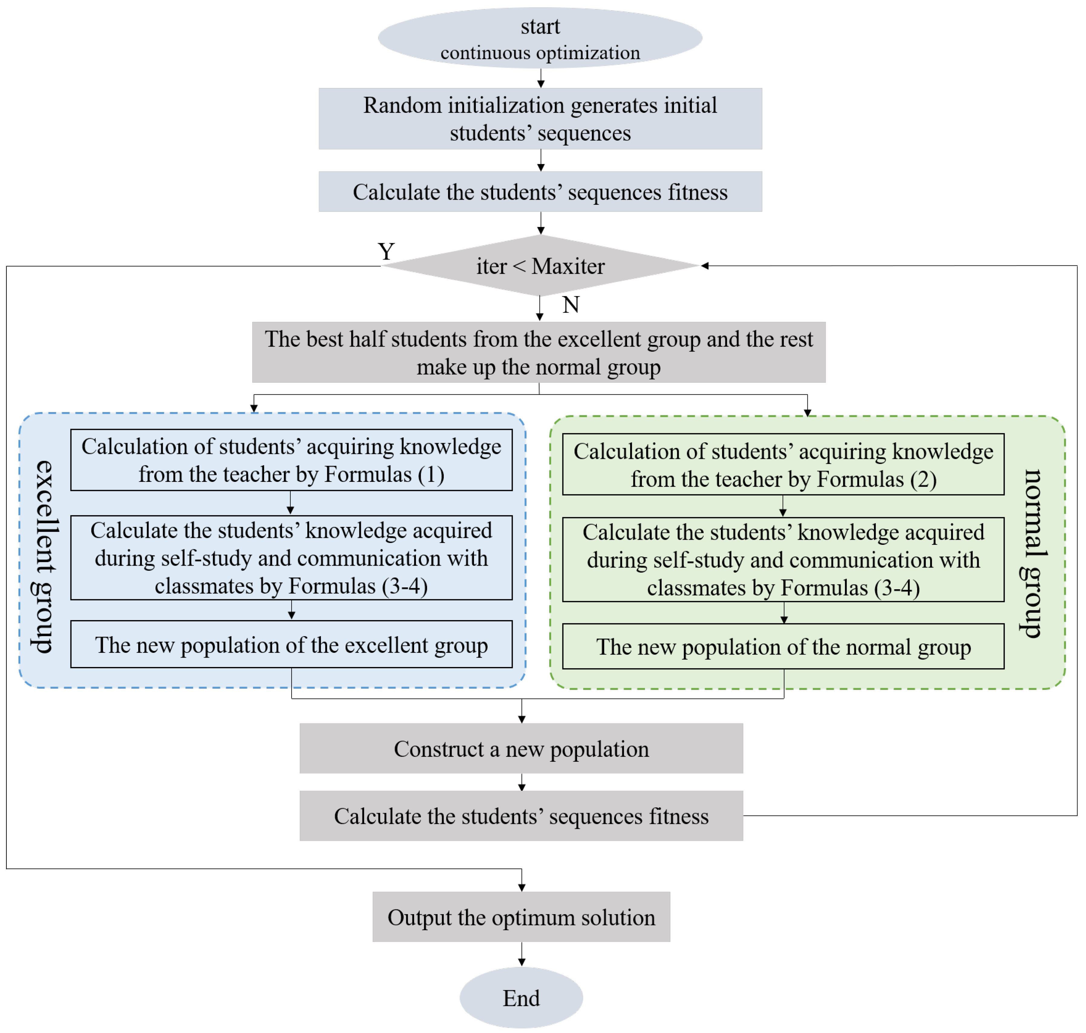
These metaheuristic algorithms solve the TSP in three main phases: initialization, crossover, and mutation [19]. In general, these metaheuristic algorithms can obtain good results when attempting to solve small-scale optimization problems. However, the larger the scale of optimization problems is, the slower the convergence speed will be, and it is also easier to fall into a local optimum [20]. 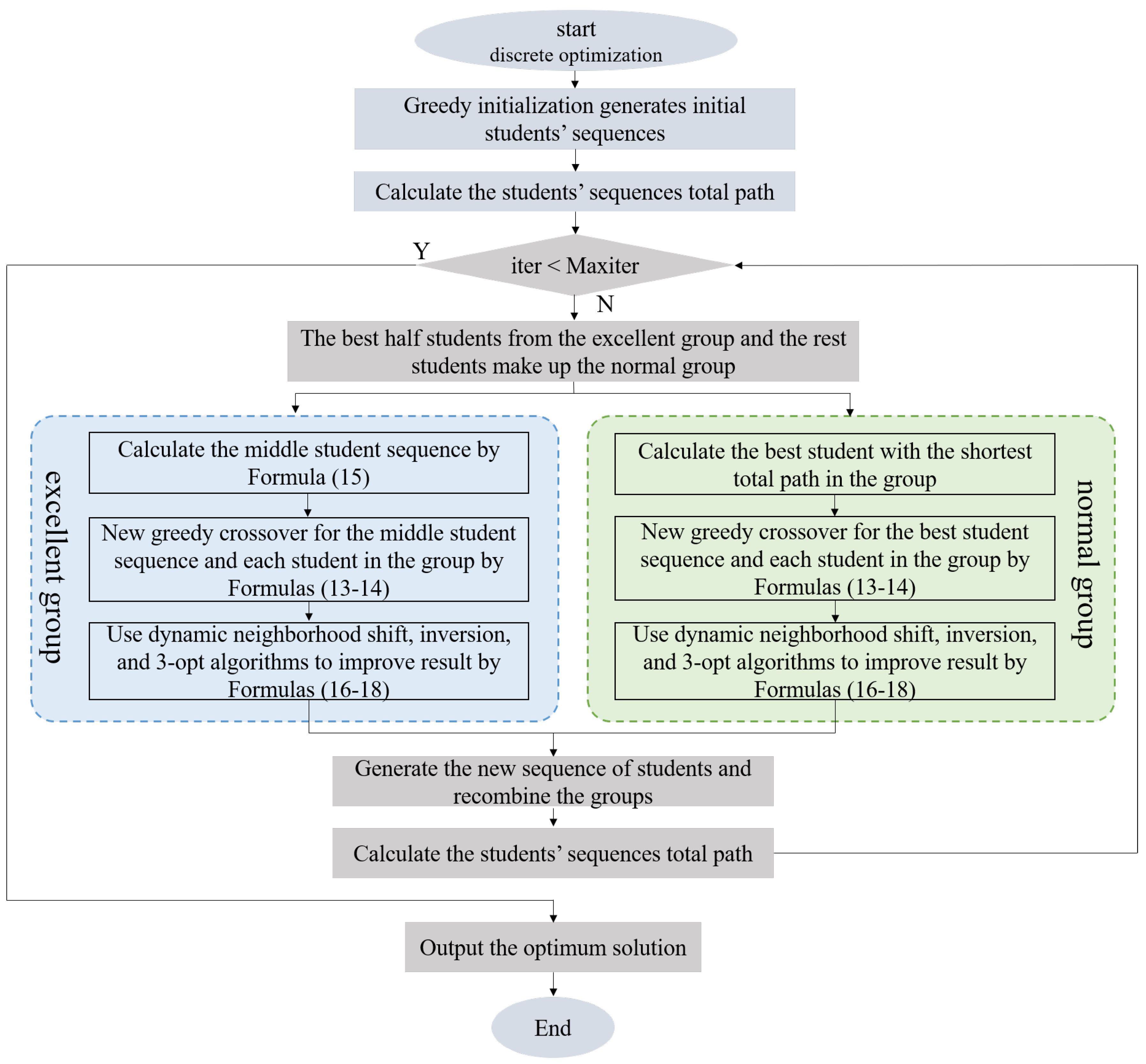Motivated by the aforementioned discussions, a novel discrete group teaching optimization algorithm (DGTOA), inspired by the group teaching optimization algorithm (GTOA) [21], is proposed to solve TSP. The DGTOA is presented in three phases in this paper. Firstly, in the initialization phase, the DGTOA generates the initial sequence for students through greedy initialization. Then, in the crossover phase, a new greedy crossover algorithm is employed to increase diversity. Finally, in the mutation phase, to balance the exploration and exploitation, this paper develops a dynamic adaptive neighborhood radius based on triangular probability selection to apply in the shift mutation algorithm, the inversion mutation algorithm, and the 3-opt mutation algorithm. In addition, to verify the performance of the DGTOA, fifteen benchmark problems in TSPLIB [22] are used to test the algorithm as well as compare it with the discrete tree seed algorithm (DTSA) [6], discrete Jaya algorithm (DJAYA) [18], ABC [7], particle swarm optimization-ant colony optimization (PSO-ACO) [23], and discrete shuffled frog-leaping algorithm (DSFLA) [24]. From the comparison results, we can conclude that the DGTOA has a comparative advantage. The main contributions of this algorithm to other algorithms in the literature are as follows:

• This study presents the first application of the GTOA in the permutation-coded discrete form.
• The DGTOA is a novel and effective discrete optimization algorithm for solving the TSP, and the comparison shows that the solutions obtained by the DGTOA have comparable performance.
• The dynamic adaptive neighborhood radius can balance the exploration and exploitation for solving the TSP.
• The DGTOA has been successfully applied to USV path planning, and the simulation results indicate that the DGTOA can provide a competitive advantage in path planning for USVs.

The remainder of the paper is arranged as follows. A literature survey on techniques to avoid falling into a local optimum and improve the optimization speed is given in Section 2. In Section 3, the original GTOA, the TSP, and the dynamic adaptive neighborhood radius model are described. After that, the DGTOA model is introduced in Section 4. Results and discussions are provided in Section 5. Finally, Section 6 concludes the study.

2. Literature Survey

The following section will focus on the current efforts of researchers to develop techniques to avoid falling into a local optimum and improve the optimization speed from the initialization, crossover, and mutation phases. Aiming at solving the TSP, related improvement techniques can be roughly introduced as follows.

The first one is improving the algorithm initialization rules to accelerate convergence. In order to speed up convergence, W. Li et al. discussed K-means clustering as a method to group individuals with similar positions into the same class to obtain the initial solution [25]. In another study, to ensure that the algorithm would execute within the given time, M. Bellmore et al. developed the nearest neighbor heuristic initialization algorithm [26]. On the basis of the nearest neighbor initialization, L. Wang et al. introduced the k-nearest neighbors’ initialization method, where the algorithm adopted a greedy approach to select the k-nearest neighbors [27]. A.C. Cinar et al. presented the initial solution of the tree during the initialization phase using the nearest neighbor and a random approach for balancing the speed and quality of its solution [6]. C. Wu et al. [28] and P. Guo et al. [29] adopted a greedy strategy for generating initialized populations to improve the optimization speed and avoid falling into a local optimum.

The second way to avoid getting trapped in the local optimum is to use crossover rules to increase diversity. For example, İlhan et al. used genetic edge recombination crossover and order crossover to avoid falling into the local optimum and improve their performances [30]. Z.H. Ahmed presented a sequential constructive crossover operator (SCX) to solve the TSP to avoid getting trapped in the local optimum [31]. In another study, Hussain et al. proposed a method based on the GA to solve TSP with a modified cycle crossover operator (CX2) [13]. In their approach, path representations have effectively balanced optimization speed and solution quality. Y. Nagata et al. devised a robust genetic algorithm based on the edge assembly crossover (EAX) operator [32]. To avoid being limited in the local optimum, the algorithm used both local and global versions of EAX.

The third one is adopting a mutation strategy to balance exploration and exploitation for solving the TSP. For instance, M. Albayrak et al. compared greedy sub-tour mutation (GSTM) with other mutation techniques. GSTM demonstrated significant advantages in polynomial-time [33]. To further avoid falling into a local optimum, A.C. Cinar et al. presented the use of swap, shift, and symmetric transformation operators for the DTSA to solve the problem of coding optimization in the path improvement phase [6]. To balance exploration and exploitation, M. Anantathanavit et al. employed K-means to cluster the sub-cities and merge them by the radius particle swarm optimization embedded into adaptive mutation, which could balance between time and accuracy [34].

Besides the main strategies for improvement mentioned above, some researchers combined a local search algorithm and a metaheuristic algorithm to avoid premature convergence and further improve the solution quality. For example, Mahi et al. developed a hybrid algorithm that combined PSO, ACO, and 3-opt algorithms, allowing it to avoid premature convergence and increase accuracy and robustness [23]. Moreover, a support vector regression approach is employed by R. Gupta et al. to solve the search space problem of the TSP [35].

Specifically, in practical ocean survey scenarios, D.V. Lyridis proposed an improved ACO with a fuzzy logic optimization algorithm for local path planning of USVs [36]. This algorithm offers considerable advantages in terms of optimal solution and convergence speed. Y.C. Liu et al. proposed a novel self-organizing map (SOM) algorithm for USV to generate sequences performing multiple tasks quickly and efficiently [37]. J.F. Xin et al. introduced a greedy mechanism and a 2-opt operator to improve the particle swarm algorithm for high-quality path planning of USV [4]. The improved algorithm was validated in a USV model in a realistic marine environment. J.H. Park et al. used a genetic algorithm to improve the mission planning capability of USVs and tested it in a simulation environment [38].

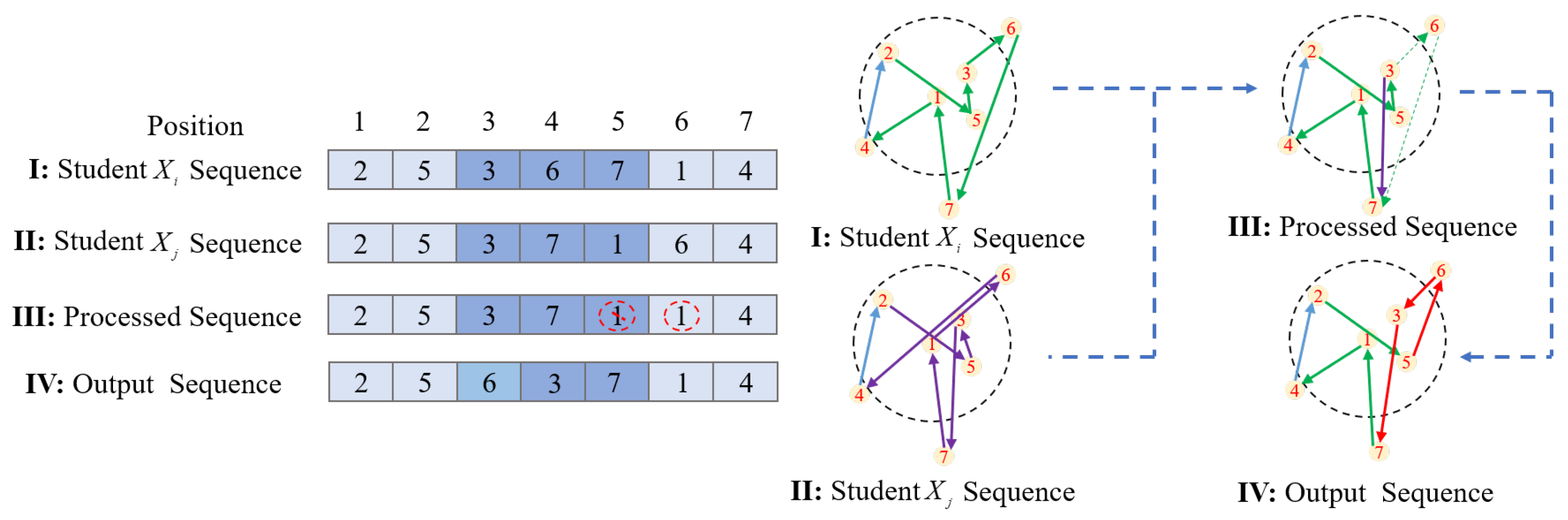
Following the literature survey, improving the algorithm initialization rules, using crossover rules, adopting a mutation strategy, combining with a local search algorithm, or all of these strategies in combination can be applied to the TSP to avoid falling into a local optimum. However, direct random crossover and global mutation are challenging in terms of convergence speed. Moreover, a higher convergence speed is required for the DGTOA to achieve rapid and optimal path planning for USVs. Thus, in contrast to the studies mentioned above, the DGTOA innovatively incorporates a dynamic adaptive neighborhood radius model, which is applied to the neighborhood mutation mode. Meanwhile, a new greedy crossover method is used to further improve TSP path exploration.

3. Background Work

In this section, we will introduce the group teaching optimization algorithm (GTOA) to solve continuous problems [21]. Meanwhile, the traveling salesman problem will be briefly described. In addition, a dynamic adaptive neighborhood radius model will be introduced.

3.1. Group Teaching Optimization Algorithm

The GTOA is inspired by the group teaching mechanism, which divides students into excellent and normal groups [39]. Depending on the results of the grouping, teachers create different teaching plans. In brief, the plans for teachers within the excellent group tend to raise the overall average, while those for students in normal groups tend to improve their individual knowledge, as shown in Formulas (1) and (2) for teachers of excellent and normal groups:

$$ExcellentGroup:x_{teacher,i}^{t+1}=x_i^t+a\times (T^t-2\times (b\times M^t+(1-b)\times x_i^t))$$

(1)

$$NormalGroup:x_{teacher,i}^{t+1}=x_i^t+2\times c\times (T^t-x_i^t)$$

(2)

where t is the number of iteration generations, $x_{teacher,i}^{t+1}$ is the knowledge acquired by student i from the teacher at time t, $x_i^t$ is the level of of student i at time t, $T^t$ is the level of knowledge of the teacher at time t, $M^t$ is the average student knowledge level of the group, and a, b, and c (0 < a, b, c < 1) are random numbers.

Combining the effects of lesson plans developed by the teacher with interaction with classmates and self-study, the knowledge learned by student i at time t can be calculated as follows:

$$x_{student,i}^{t+1}=\left\{\begin{array}{cc}\hfill x_{teacher,i}^{t+1}+rand\times (x_{teacher,i}^{t+1}-x_{teacher,j}^{t+1})+rand\times (x_{teacher,i}^{t+1}-x_i^t),f\left(x_{teacher,i}^{t+1}\right)<f\left(x_{teacher,i}^{t+1}\right)\hfill & \\ \hfill x_{teacher,i}^{t+1}-rand\times (x_{teacher,i}^{t+1}-x_{teacher,j}^{t+1})+rand\times (x_{teacher,i}^{t+1}-x_i^t),f\left(x_{teacher,i}^{t+1}\right)\ge f\left(x_{teacher,i}^{t+1}\right)\hfill \end{array}\right.$$

(3)

$$x_i^{t+1}=\left\{\begin{array}{cc}\hfill x_{teacher,i}^{t+1},f\left(x_{teacher,i}^{t+1}\right)<f\left(x_{student,i}^{t+1}\right)\hfill & \\ \hfill x_{student,i}^{t+1},f\left(x_{teacher,i}^{t+1}\right)\ge f\left(x_{student,i}^{t+1}\right)\hfill \end{array}\right.$$

(4)

where $x_{student,i}^{t+1}$ is the knowledge acquired by student i at time t, and $x_{teacher,j}^{t+1}$ is the knowledge acquired by student j from the teacher at time t, j is not equal to i. Following the completion of the learning process at time t, two groups are combined and regrouped by their acquisition level until the termination condition is met, $f\left(x\right)$ is the normal distribution [39] and $x_i^{t+1}$ represents the knowledge of student i at time $t+1$. The process of the GTOA can be seen from Figure 2 and the pseudo-code of the GTOA is implemented in Algorithm 1.

Algorithm 1: Pseudo-code of GTOA

Figure 2. Flowchart of group teaching optimization algorithm.

3.2. Traveling Salesman Problem (TSP)

The TSP can be represented by the complete graph $G=(V,E)$, where V is the set of cities and E is the edges connecting them. In the Hamiltonian loop, once a city is taken as a starting point, all cities are visited only once and the loop eventually returns to the starting city. The target should be to make the Hamiltonian loop as short as possible [40].

$$c_{ij}=\left\{\begin{array}{cc}1,\hfill & Travellingsalesmanthroughtheedge(i,j)\\ 0,\hfill & Others\end{array}\right.$$

(5)

$$min\sum _{\begin{array}{c}i\in V\end{array}}\sum _{\begin{array}{c}j\in V\end{array}}{c}_{ij}{d}_{ij}$$

(6)

$$\sum _{i=1,j\in V}^D{c}_{ij}=\sum _{j=1,i\in V}^D{c}_{ij}=1$$

(7)

$$\sum _{\begin{array}{c}i\in S\end{array}}\sum _{\begin{array}{c}j\in S\end{array}}{c}_{ij}\le \left|S\right|-1\forall S\subset V,\left|S\right|\ge 2$$

(8)

where $d_{ij}$ is the distance of the edge (i, j) and D indicates the total number of cities to be visited; Formula (7) guarantees that each city is visited only once; Formula (8) guarantees that the result is a Hamiltonian loop.

3.3. Dynamic Adaptive Neighborhood Radius

To improve accuracy and efficiency, this paper proposes a method of a dynamic adaptive neighborhood radius, which incorporates the exponential function into the iterative generations and tanh functions to balance linear and nonlinear relationships. A description of the model design can be decided through:

$$r^z=tanh{e}^{(-\frac{iter}{Maxiter}+0.1)}\left(\frac{r_{avg}^z-d_{min}}{d_{avg}-d_{min}}\right)(r_{max}^z-r_{min}^z)+r_{min}^z,z=1,2,\cdots ,N$$

(9)

where z is the current city and $r_{max}^z$, $r_{min}^z$, and $r_{avg}^z$ are the maximum, minimum, and average distance between the unvisited city and current city, respectively. $d_{min}$ and $d_{avg}$ represent the minimum and average distance between all cities, respectively, $Maxiter$ is the maximum number of iterations, and iter is the current number of iterations.

The triangular probability selection model [41] increases the probability of selecting relatively close individuals, as well as ensures that individuals from further away have a chance of being selected in the neighborhood. The details are as follows: firstly, the neighboring cities are sorted by distance from the current city z in descending order, and the probability of a city i being chosen is shown in Formula (10), where n is the number of neighboring cities. Then a random number k is generated according to Formula (11). Finally, a city $c_m$ is selected as the next target city of the current city z according to Formula (12):

$$P_i=2(n+1-i)/\left(n(n+1)\right)1\le i\le n$$

(10)

$$k\in [0,n{P}_1+(n-1)P_2+\cdots +P_n]$$

(11)

$$\left\{\begin{array}{cc}\hfill c_1\hfill & \hfill k\le P_1\hfill \\ \hfill c_m\hfill & \hfill (m-1)P_1+\cdots +P_{m-1}<k\le m{P}_1+\cdots +P_m,1<m\le n\hfill \end{array}\right.$$

(12)

where $c_m$ is the m-th city of the data sorted in descending order by distance from the current city z.

4. Discrete Group Teaching Optimization Algorithm Detail Design

In this section, the discrete group teaching optimization algorithm will be introduced to solve TSP. Meanwhile, a new greedy crossover algorithm, a middle student algorithm, a dynamic neighborhood shift mutation algorithm, a dynamic neighborhood inversion mutation algorithm, and a dynamic neighborhood 3-opt mutation algorithm will be described. Related details will be introduced in the following subsections.

4.1. Discrete Group Teaching Optimization Algorithm

In discrete optimal problems, the DGTOA is modified in two stages. For the first stage, the greedy principle [6] is used to generate the initial students’ sequences. For the later stage, students are divided into two groups, with the top 50 percent of students on the total path assigned to the excellent group and the rest to the normal group. The following process is shown in Figure 3.

Figure 3. Flowchart of discrete group teaching optimization algorithm.

In the excellent group, based on Section 3.1, the group focuses on improving the overall performance. The related design process for the DGTOA can be described as follows. (1) The middle student sequence is generated from the whole group of students’ sequences by the middle student algorithm. (2) Each student in the group is processed with the middle sequence using the new greedy crossover. (3) The dynamic neighborhood shift mutation algorithm, the dynamic neighborhood inversion mutation algorithm, and the dynamic neighborhood 3-opt mutation algorithm are used to improve the optimization results after greedy crossover. (4) Finally, the new sequences of the excellent group are output, as shown in Figure 3 in blue.

The normal group is designed as follows. (1) The shortest student sequence by selecting from all students in the normal group. (2) Using a new greedy crossover, each student in the group is processed with the shortest path sequence. (3) The dynamic neighborhood shift mutation algorithm, the dynamic neighborhood inversion mutation algorithm, and the dynamic neighborhood 3-opt mutation algorithm are used to improve the optimization results after greedy crossover. (4) Finally, the new sequences of the normal group are output, as shown in Figure 3 in green.

Then, combine the excellent group and the normal group and determine whether the termination condition is met. If not, the next step is to return to the excellent group and continue the later stage; otherwise, the final result will be output from the combining group as the global DGTOA optimum value, as shown in Figure 3 in gray. The corresponding pseudo-code is shown in Algorithm 2.

Algorithm 2: Pseudo-code of DGTOA

4.2. New Greedy Crossover Algorithm

To begin with, two positions m and n are randomly selected from the students $X_i$ and $X_j$, and the distance ${\lambda }_{mn}$ between two positions is calculated using Formula (14). Then the sequence is selected between positions m and n from the students $X_i$ and $X_j$ with a smaller length replacement to $X_i$ between positions m and n. Additionally, the repeated city is removed between positions m and n. Finally, the rest of the cities will be inserted into a new sequence according to the greedy rule, as follows:

$$x_i^k=\left\{\begin{array}{cc}\hfill x_i^{k+N}-N<k<1\hfill & \\ \hfill x_i^{k}1\le k\le N\hfill & \\ \hfill x_i^{k-N}N<k\le 2N\hfill \end{array}\right.$$

(13)

$${\lambda }_{mn}=\left\{\begin{array}{cc}\hfill {\displaystyle \sum _{k=m}^{n-1}}d(x_i^k,x_i^{k+1})m<n\hfill & \\ \hfill {\displaystyle \sum _{k=n}^{m-1}}d(x_i^k,x_i^{k+1})n<m\hfill \end{array}\right.$$

(14)

$$min\sum _{k=1}^{re-1}d(x_i^k,x_i^{k+1})+\sum _{k=re}^{N_i^{re}-1}d(x_i^k,x_i^{k+1})$$

(15)

where $d(x_i^m,x_i^n)$ is the distance between cities $x_i^m$ and $x_i^n$, the subscript denotes the student number, ranging from 1 to M, in which M is the total number of students. The superscript denotes the student’s corresponding sequence position number, ranging from 1 to N, in which N is the total number of cities. In addition, $re$ is the unvisited city position and $N_i^{re}$ is the current sequence length of student $X_i$. For instance, positions 3 and 5 are randomly selected from the students $X_i$ and $X_j$ (as seen from Figure 4). Then the smaller distance (positions 3->7->1) is selected and the repeated city 1 is removed. Finally, the unvisited city 6 is added to the output sequence in a greedy rule.

Figure 4. New greedy crossover algorithm.

4.3. Middle Student Algorithm

The sequence of the middle student is obtained based on the form of most of the common cities, for N cities, M students can be established as in Formula 16.

$$Center(X_1,X_2,\cdots ,X_M)={Most}_{i=1,2,\cdots ,M}(x_i^1,x_i^2,\cdots ,x_i^N)$$

(16)

where $x_i^N$ denotes the city corresponding to position N from the i-th student sequence. The sequence of a middle student is processed in position order. First, delete cities that have been visited, and then, based on the occurrence frequency of the remaining cities, select the city with the highest frequency to fill the corresponding position. If more than one city with the highest frequency is presented, randomly select one to fill this position. Additionally, if all the cities in this position are deleted, select cities at random from the rest of the sequence until the whole sequence is done.

As shown in Figure 5, for instance, in the first case, the cities with the highest frequency in positions 2, 3, 4, 5, and 7 are selected based on the statistics of the remaining cities’ frequencies. In the second case, more than one city is presented with the highest frequency in position 1, and thus city 2 is randomly chosen. In the third case, all cities in position 6 are deleted, a city 6 is randomly selected from the rest cities to fill the sequence.

Figure 5. Middle student algorithm.

4.4. Dynamic Neighborhood Shift Mutation Algorithm

A position n is randomly selected from a sequence of student $X_i$. A city is selected from the dynamic adaptive neighborhood radius $r^z$ of the city corresponding to position m in the sequence by the triangular probability selection model, where $x_n$ is the position n corresponding to the city. After that, the sequence’s city corresponding to position m is shifted to position n. Finally, the value of the left and right change to the path distance $\Delta {\lambda }_1$ and $\Delta {\lambda }_2$ are calculated, respectively.

$$\left\{\begin{array}{cc}\hfill \Delta {\lambda }_1=(d(x_i^{m-1},x_i^n)+d(x_i^m,x_i^n)+d(x_i^{n-1},x_i^{n+1}))-(d(x_i^{n-1},x_i^n)+d(x_i^n,x_i^{n+1})+d(x_i^{m-1},x_i^m))\hfill & \\ \hfill \Delta {\lambda }_2=(d(x_i^m,x_i^n)+d(x_i^{m+1},x_i^n)+d(x_i^{n-1},x_i^{n+1}))-(d(x_i^{n-1},x_i^n)+d(x_i^n,x_i^{n+1})+d(x_i^m,x_i^{m+1}))\hfill \end{array}\right.$$

(17)

where $x_i^m$ and $x_i^n$ are the cities corresponding to positions m and n in the i-th student sequence, respectively. Accordingly, if $\Delta {\lambda }_1\le \Delta {\lambda }_2$, move $x_i^n$ between $x_i^{m-1}$ and $x_i^m$. If not, move $x_i^n$ between $x_i^m$ and $x_i^{m+1}$, as shown in Figure 6.

Figure 6. Dynamic neighborhood shift mutation.

4.5. Dynamic Neighborhood Inversion Mutation Algorithm

In the sequence of student i, a position n is randomly selected. From the dynamic adaptive neighborhood radius of the city corresponding to position n, one city is selected and its position m is recorded. In addition, the positions m and n in the sequence are compared, and the smaller value is assigned to $min$, while the larger value is assigned to $max$, as determined by Formula (18), and the change in distance before and after the inversion mutation is calculated as $\Delta {\lambda }_3$, $\Delta {\lambda }_4$, $\Delta {\lambda }_5$, and $\Delta {\lambda }_6$:

$$\left\{\begin{array}{cc}\hfill x_i^{min}=x_i^m,x_i^{max}=x_i^{n}m<n\hfill & \\ \hfill x_i^{min}=x_i^n,x_i^{max}=x_i^{m}n<m\hfill \end{array}\right.$$

(18)

$$\left\{\begin{array}{cc}\hfill \Delta {\lambda }_3=(d(x_i^{max-1},x_i^{min-1})+d(x_i^{max},x_i^{min}))-(d(x_i^{max-1},x_i^{max})+d(x_i^{min-1},x_i^{min}))\hfill & \\ \hfill \Delta {\lambda }_4=(d(x_i^{max-1},x_i^{min})+d(x_i^{max},x_i^{min+1}))-(d(x_i^{max-1},x_i^{max})+d(x_i^{min},x_i^{min+1}))\hfill & \\ \hfill \Delta {\lambda }_5=(d(x_i^{max},x_i^{min-1})+d(x_i^{max+1},x_i^{min}))-(d(x_i^{max},x_i^{max+1})+d(x_i^{min-1},x_i^{min}))\hfill & \\ \hfill \Delta {\lambda }_6=(d(x_i^{max},x_i^{min})+d(x_i^{max+1},x_i^{min+1}))-(d(x_i^{max},x_i^{max+1})+d(x_i^{min},x_i^{min+1}))\hfill \end{array}\right.$$

(19)

For instance, if $\Delta {\lambda }_3<0$, reverse the order of $x_i^{min}\sim x_i^{max-1}$; if $\Delta {\lambda }_4<0$, reverse the order of $x_i^{min+1}\sim x_i^{max-1}$; if $\Delta {\lambda }_5<0$, reverse the order of $x_i^{min}\sim x_i^{max}$; if $\Delta {\lambda }_6<0$, reverse the order of $x_i^{min+1}\sim x_i^{max}$. As depicted in Figure 7a–d.

Figure 7. Dynamic neighborhood inversion mutation. (a) Reverse the order $x_i^{min}\sim x_i^{max-1}$. (b) Reverse the order $x_i^{min+1}\sim x_i^{max-1}$. (c) Reverse the order $x_i^{min}\sim x_i^{max}$. (d) Reverse the order $x_i^{min+1}\sim x_i^{max}$.

4.6. Dynamic Neighborhood 3-opt Mutation Algorithm

The 3-opt algorithm has a strong local search capability. However, directly processing all cities would take a long computational time, and the amount of time would increase as the number of cities increased. Therefore, we present a method of combining dynamic neighborhood radius with 3-opt to maximize its ability to find local optimal solutions: by selecting a position n randomly in the sequence of students i and then applying the 3-opt algorithm to determine the next city within the dynamic adaptive neighborhood radius of the cities.

5. Results and Discussions

The DGTOA with dynamic adaptive neighborhood optimization is tested using 15 benchmark TSP cases taken from TSPLIB [22]. Most of the instances in TSPLIB have been solved, and the optimum values are displayed. The numbers in the problem names indicate the city numbers (e.g., the eil51 benchmark problem means that the problem has 51 cities). Testing is performed using fifteen benchmark problems, which are divided into three categories: small-scale, medium-scale, and large-scale based on city numbers, respectively. For example, the case with less than 100 cities is considered a small-scale benchmark problem; the case with more than 100 but less than 200 cities is a medium-scale benchmark problem, and the case with more than 200 but less than 300 cities is a large-scale benchmark problem. Each of the experiments in this section is carried out 25 times independently, with the best results, mean results, and standard deviation (Std Dev) values produced by the algorithm having been recorded, and the best optimum results are written in bold font in the result tables. The relative error (RE) is calculated as follows:

$$RE=\frac{R-O}{O}\times 100\%$$

(20)

where R is the obtained length (mean of 25 repeats) by the DGTOA, and O is the optimum value of the problem. The optimum problems and their values are given in Table 1 [18,42]. All experiments are carried out using a Windows 11 Professional Insider Preview laptop with an Intel (R) Core (TM) i7-7700HQ 2.8 GHz processor and 16 GB of RAM, with the scripts being written in MATLAB 2021a. The following is a series of experiments in which the maximum number of iterations is 1000 and the number of students is 100.

Table 1. Number of cities and optimum tour lengths of the problems.

Problem	Number of Cities	Optimum Tour Length
eil51	51	428.87
berlin52	52	7544.37
st70	70	677.11
pr76	76	108,159.44
eil76	76	545.38
kroa100	100	21,285.44
krob100	100	22,141
kroc100	100	20,749
krod100	100	21,294
kroe100	100	22,068
eil101	101	642.31
ch150	150	6532.1
pr152	152	73,683.6
kroa200	200	29,460
tsp225	225	3859

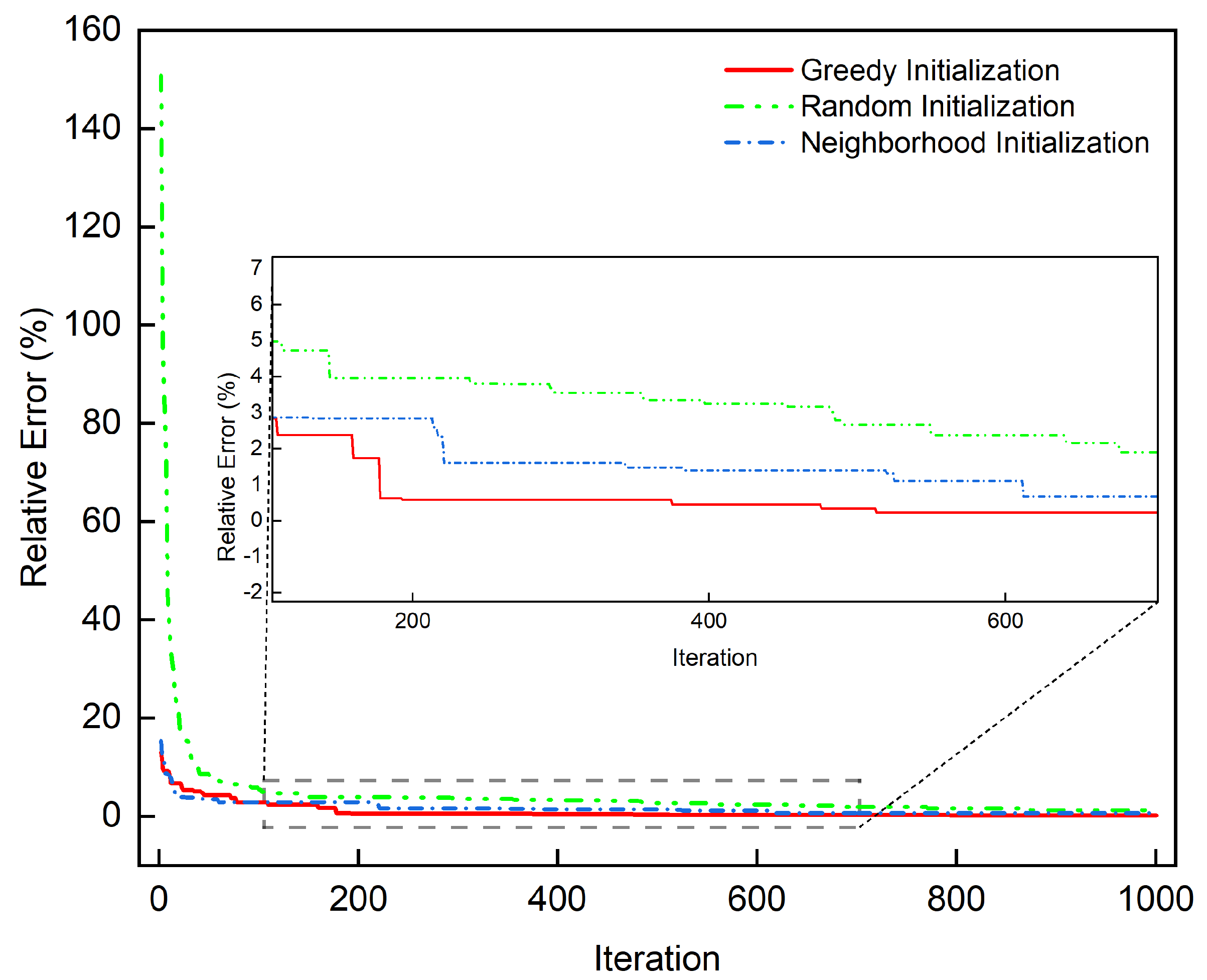
5.1. Experiment 1: Comparisons with Random Initialization, Neighborhood Initialization, and Greedy Initialization

The experiment uses fifteen benchmark problems to evaluate the efficacy of random initialization, neighborhood initialization, and greedy initialization to solve TSP. The obtained results are shown in Table 2.

Table 2. Comparisons with random initialization, neighborhood initialization, and greedy initialization on fifteen benchmark problems.

Problems	Random initialization				Neighborhood Initialization				Greedy Initialization
	Mean	Std Dev	RE (%)		Mean	Std Dev	RE (%)		Mean	Std Dev	RE (%)
eil51	430.35	1.29	0.34		429.92	0.92	0.24		429.78	0.99	0.21
berlin52	7544.37	0	0		7544.37	0	0		7544.37	0	0
st70	681.3	3.38	0.62		677.11	0.02	0		677.11	0.02	0
pr76	110,499	1214.54	2.16		108,344	331.36	0.17		108,298.6	287.72	0.13
eil76	554.09	2.61	1.6		549.84	1.81	0.82		549.44	1.81	0.74
kroa100	21,466.9	97.44	0.85		21,285.8	1.75	0		21,286.16	2.43	0
krob100	22,410	130.91	1.22		22,235.4	32.65	0.43		22,216.7	48.05	0.34
kroc100	20,974.1	155.93	1.08		20,809	44.61	0.29		20,778.18	37.53	0.14
krod100	21,621.9	143.5	1.54		21,485.2	64.79	0.9		21,456.83	55.58	0.76
kroe100	22,330.1	97.78	1.19		22,169.9	48.77	0.46		22,152.85	33.32	0.38
eil101	651.89	2.88	1.49		647.08	2.92	0.74		646.75	2.62	0.69
ch150	6763.4	60.96	3.54		6554.55	5.28	0.34		6554.4	3.93	0.34
pr152	74,968.6	386.56	1.74		74,356.1	175.35	0.91		74,408.66	225.48	0.98
kroa200	30,995	213.99	5.21		29,631.1	54.81	0.58		29,606.35	70.2	0.5
tsp225	4018.67	25.94	4.14		3940.41	19.73	2.11		3938.95	16.76	2.07

According to the bold part in Table 2, in terms of mean and RE, the optimization solutions produced by neighborhood initialization and greedy initialization have considerable advantages over random initialization. On the other hand, by analyzing the neighborhood initialization as well as greedy initialization, it is evident from Table 2 that the greedy initialization has a slight advantage in 11 instances. However, the neighborhood initialization has a slight performance on eil101 and pr152. For further analysis of the three initialization methods iterative process, the convergence RE plots of the middle-scale eil101 and large-scale tsp225 benchmark problems are given in Figure 8 and Figure 9, which are used to compare the convergence processes of random initialization, neighborhood initialization, and greedy initialization.

Figure 8. RE curves with random initialization, neighborhood initialization, and greedy initialization for different iteration periods based on eil101.

Figure 9. RE curves with random initialization, neighborhood initialization, and greedy initialization for different iteration periods based on tsp225.

According to Figure 8, the neighborhood initialization and greedy initialization show a considerable advantage in the initial solution over random initialization. For random initialization, it takes 500 generations to reach an RE of less than 3%, but for neighborhood initialization and greedy initialization, they take only 100 generations to satisfy convergence. Compared to neighborhood initialization, greedy initialization can achieve an RE of less than 1% within 200 generations, whereas neighborhood initialization takes 600 generations to achieve an RE of less than 1%.

As seen in Figure 9, compared to neighborhood initialization and greedy initialization, the random initialization method has a certain gap in the initial results as well as the final optimization results, and the convergence to an RE of less than 5% has a larger gap. Moreover, the RE of greedy initialization declines less than 3% faster than neighborhood initialization. Hence the DGTOA uses a greedy rule in the initialization phase.

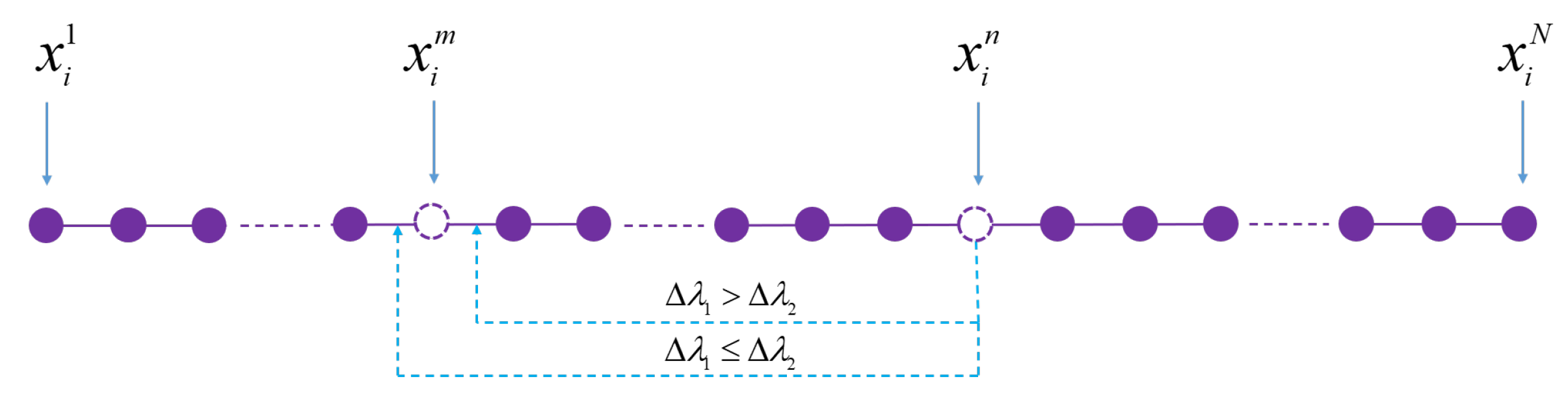
5.2. Experiment 2: Comparisons with Adaptive Neighborhood Mutation and Dynamic Adaptive Neighborhood Mutation

To compare the adaptive neighborhood radius and the dynamic adaptive neighborhood radius during the mutation phase. The adaptive neighborhood radius is assigned $iter$ as a value of 500 and fixed (Formula (9)). Fifteen benchmark problems are used to evaluate the effectiveness of the two neighborhood radius methods to solve the TSP, with all parameters except $iter$ set the same each time. The results are shown in Table 3.

Table 3. Comparisons with adaptive neighborhood mutation and dynamic adaptive neighborhood mutation.

Problems	Adaptive Neighborhood Mutation					Dynamic Adaptive Neighborhood Mutation
	Mean	Std Dev	RE (%)	Best		Mean	Std Dev	RE (%)	Best
eil51	429.49	0.75	0.15	428.98		429.78	0.99	0.21	428.87
berlin52	7544.37	0	0	7544.37		7544.37	0	0	7544.37
st70	677.12	0.02	0	677.11		677.11	0.02	0	677.11
pr76	108,542	447.33	0.35	108,159		108,298.6	287.72	0.13	108,159.4
eil76	549.33	2.01	0.72	545.39		549.44	1.81	0.74	545.97
kroa100	21,286.9	7.12	0.01	21,285.4		21,286.16	2.43	0	21,285.4
krob100	22,251.9	37.42	0.5	22,178.6		22,216.7	48.05	0.34	22,139.07
kroc100	20,824.7	55.15	0.36	20,750.8		20,778.18	37.53	0.14	20,750.76
krod100	21,463	52.66	0.79	21,345.5		21,456.83	55.58	0.76	21,323.48
kroe100	22,157.1	34.25	0.4	22,119.9		22,152.85	33.32	0.38	22,115.61
eil101	647.4	3.11	0.79	641.88		646.75	2.62	0.69	641.23
ch150	6552.5	8.15	0.31	6530.9		6554.4	3.93	0.34	6545.16
pr152	74,432.9	250.23	1.02	74,128.6		74,408.66	225.48	0.98	73,936.17
kroa200	29,667.3	61.81	0.7	29,560		29,606.35	70.2	0.5	29,405.72
tsp225	3950.47	18.52	2.37	3911.3		3938.95	16.76	2.07	3912.3

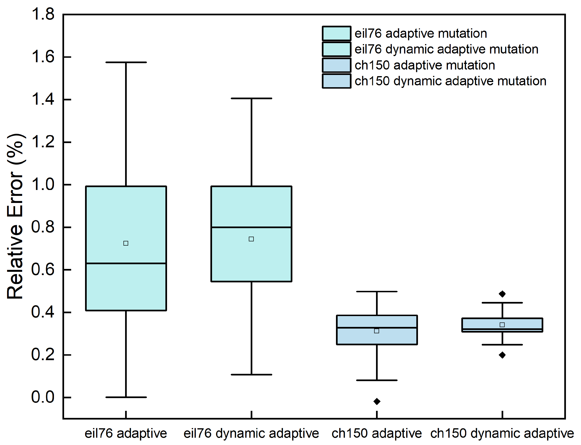
As seen from Table 3, the dynamic adaptive neighborhood mutation has a promising advantage over the adaptive neighborhood mutation in terms of mean and RE values, with an advantage in twelve of the fifteen benchmark problems and only a slight disadvantage in eil76 and ch150. Moreover, a box plot of the eil76 and ch150 benchmark problems with the dynamic adaptive neighborhood mutation and the adaptive neighborhood mutation for 25 tests is shown so that the results can be fully analyzed.

From Figure 10, the results from the dynamic adaptive neighborhood mutation are more concentrated. In contrast, the adaptive neighborhood mutation is less stable and thus presents a smaller final average result than the dynamic adaptive neighborhood mutation. For instance, the average optimal value in ch150 in Figure 10 is much smaller than the dynamic adaptive neighborhood mutation. However, the middle, upper quartile, and upper edge are larger than the dynamic adaptive neighborhood mutation. Therefore, the dynamic adaptive neighborhood mutation is optimal for the mutation phase due to its stability and efficiency.

Figure 10. Box plot for the eil76 and ch150 benchmark problems with dynamic adaptive neighborhood mutation and adaptive neighborhood mutation.

5.3. Experiment 3: Comparisons with the DJAYA, DTSA, ABC, PSO-ACO, and DSFLA

The DJAYA [18], DTSA [6], ABC [7], PSO-ACO [23], and DSFLA [24] are used to compare with the DGTOA, and the comparison results regarding RE values are shown in Table 4. The results are taken directly from the related papers for the DJAYA, DTSA, ABC, PSO-ACO, and DSFLA.

Table 4. Comparisons with the DJAYA, DTSA, ABC, PSO-ACO, and DSFLA.

SL	Problem	RE (%)
		DJAYA	DTSA	ABC	PSO-ACO	DSFLA	DGTOA
1	eil51	2.64	3.51	0.28	0.11	0.1	0.21
2	berlin52	0.48	0.02	0	0.02	0	0
3	st70	3.72	4.66	0.66	0.47	0	0
4	pr76	4.71	6.26	0.43	-	-	0.13
5	eil76	5.1	6.09	-	0.06	0.2	0.74
6	kroa100	1.99	1.06	0.98	0.77	0.14	0
7	krob100	3.76	4.51	-	-	-	0.34
8	kroc100	4.59	5.15	-	-	0.11	0.14
9	krod100	6.28	7.88	-	-	-	0.76
10	kroe100	2.33	1.83	-	-	-	0.38
11	eil101	5.46	7.41	2.9	0.59	0.62	0.69
12	ch150	1.63	3.32	-	0.55	0.53	0.34
13	pr152	-	-	-	-	0.39	0.98
14	kroa200	-	-	-	0.95	1.03	0.5
15	tsp225	6.12	9.93	6.83	-	-	2.07
Optimal number/ratio (%)		0/0	0/0	1/14.29	2/25	5/66.67	10/66.67

As shown in Table 4, the DGTOA has competitive performance, obtaining optimal solutions for 10 of the 15 benchmark problems, representing 66.77% of all test cases. In terms of the quality of the solutions, DGTOA is obviously superior to the DJAYA, DTSA, and ABC, as well as 6 of 8 (75%) and 7 of 10 (70%) better than PSO-ACO and the DSFLA, respectively (i.e., the DSFLA has the same RE value on the Berlin52 and St70 benchmark problems). The test results show that the ABC, PSO-ACO, DSFLA, and DGTOA perform well at a small scale, but as the scale increases, the performance of the ABC algorithm decreases significantly. Meanwhile, for the tsp225 benchmark problem, the algorithm test result RE value is higher than 5% at a large scale. In addition, PSO-ACO, the DSFLA, and the DGTOA perform similarly on small and medium scales. In contrast, for large-scale kroa200, the DGTOA has a significant advantage over PSO-ACO and the DSFLA. Therefore, the DGTOA has a considered performance in fifteen benchmark problems.

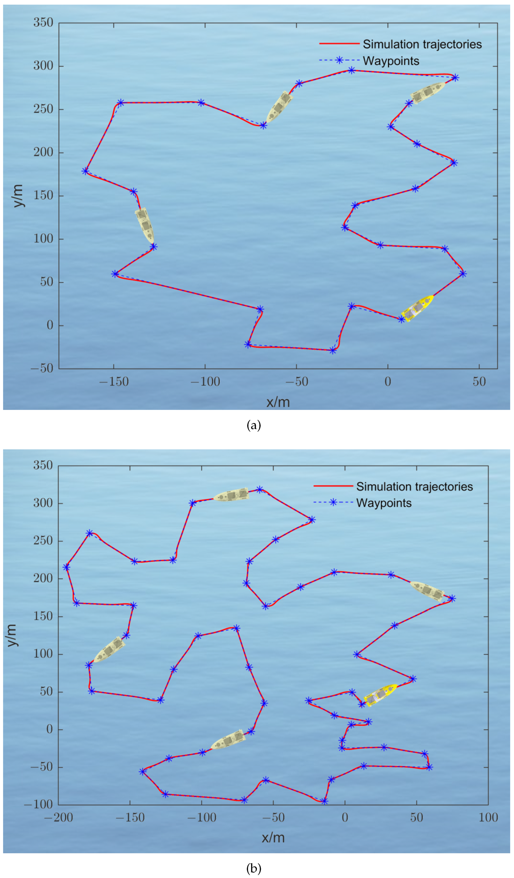
5.4. Experiment 4: Case Study with USV Path Planning

To evaluate the effectiveness of the designed DGTOA in the context of USV path planning, the USV model published in [43] is used to verify the algorithm’s performance in MATLAB. The control algorithm is derived from the line-of-sight guidance laws described in [44,45]. For planning the path, 25 and 50 target waypoints are randomly generated, and then the relevant waypoints are entered into DGTOA. Finally, the optimized paths are provided to the simulated USV for tracking control experiments. The results are shown in Figure 11a,b, where the blue stars represent the waypoints and the solid red line indicates the USV tracking trajectory with the speed of 1 m/s. The generated paths are of satisfactory lengths, and no paths cross, significantly reducing the time and energy required for USV. Furthermore, the convergence RE plots of the 25 and 50 target waypoints are shown in Figure 12. When 25 target waypoints are considered, the DGTOA converges to the optimum after only three iterations. Meanwhile, for 50 target waypoints, the DGTOA converges to the optimum in only eight generations. From the two waypoint cases, the DGTOA converges to the optimal solution in 0.47 s and 0.58 s, respectively. In general, the DGTOA has good performance in terms of optimal solution and convergence speed.

Figure 11. Simulated USV path tracking results at 25 and 50 waypoints. (a) Simulated USV path tracking results at 25 waypoints. (b) Simulated USV path tracking results at 50 waypoints.

Figure 12. RE curves using the DGTOA for 25 and 50 waypoints.

6. Conclusions

To efficiently solve large-scale waypoint route planning issues, a novel DGTOA method is proposed for USVs. The DGTOA proposes a dynamic adaptive neighborhood radius strategy to balance exploration and exploitation. In the initialization phase, the DGTOA generates initial student sequences using greedy initialization to accelerate the convergence. During the crossover phase, when the new greedy crossover method is used, every student in the group is processed with the shortest sequence and the middle student sequence corresponding to the normal group and the excellent group, respectively. In the mutation phase, the dynamic neighborhood shift mutation algorithm, the dynamic neighborhood inversion mutation algorithm, and the dynamic neighborhood 3-opt mutation algorithm all use the dynamic adaptive neighborhood radius based on triangular probability selection to increase diversity.

In order to verify the effectiveness of the DGTOA, fifteen benchmark problems from TSPLIB are used as benchmarks for testing. In the study, the effects of random initialization, neighborhood initialization, and greedy initialization on the DGTOA are also discussed. In terms of quality and convergence speed, greedy initialization for the DGTOA has an advantage over random initialization and neighborhood initialization. What is more, the dynamic adaptive neighborhood mutation has promising performance relative to the adaptive neighborhood mutation in terms of mean and RE values. In comparison with the DJAYA, DTSA, ABC, PSO-ACO, and DSFLA on 15 benchmark problems from TSPLIB, the DGTOA shows obvious superiority over the DJAYA, DTSA, ABC, and is 75% and 70% better than PSO-ACO and the DSFLA, respectively. Furthermore, the DGTOA has been successfully applied to the path planning for a USV and the results indicate that the DGTOA performs well in terms of optimal solution and convergence speed. Therefore, the proposed DGTOA can provide a competitive advantage in path planning for USVs.

Nevertheless, this study also has some limitations. Firstly, the computation time and results of the algorithm are not optimal, especially as the problem scale increases. Secondly, the DGTOA will be modified to plan routes for multiple unmanned surface vehicles.

References

- Nantogma, S.; Pan, K.; Song, W.; Luo, W.; Xu, Y. Towards Realizing Intelligent Coordinated Controllers for Multi-USV Systems Using Abstract Training Environments. J. Mar. Sci. Eng. 2021, 9, 560. [Google Scholar] [CrossRef]
- Xin, J.F.; Zhong, J.B.; Li, S.X.; Sheng, J.L.; Cui, Y. Greedy mechanism based particle swarm optimization for path planning problem of an unmanned surface vehicle. Sensors 2019, 19, 4620. [Google Scholar] [CrossRef]
- Wang, Z.; Yang, S.Y.; Xiang, X.B.; Antonio, V.; Nikola, M.; Ðula, N. Cloud-based mission control of USV fleet: Architecture, implementation and experiments. Control. Eng. Pract. 2021, 106, 104657. [Google Scholar] [CrossRef]
- Fan, J.; Li, Y.; Liao, Y.; Jiang, W.; Wang, L.F.; Jia, Q.; Wu, H.W. Second path planning for unmanned surface vehicle considering the constraint of motion performance. J. Mar. Sci. Eng. 2019, 7, 104. [Google Scholar] [CrossRef]
- Ege, E.; Ankarali, M.M. Feedback Motion Planning of Unmanned Surface Vehicles via Random Sequential Composition. Trans. Inst. Meas. Control. 2019, 41, 3321–3330. [Google Scholar] [CrossRef]
- Cinar, A.C.; Korkmaz, S.; Kiran, M.S. A discrete tree-seed algorithm for solving symmetric traveling salesman problem. Eng. Sci. Technol. Int. 2020, 23, 879–890. [Google Scholar] [CrossRef]
- Kıran, M.S.; İşcan, H.; Gündüz, M. The analysis of discrete artificial bee colony algorithm with neighborhood operator on traveling salesman problem. Neural Comput. 2013, 23, 9–21. [Google Scholar] [CrossRef]
- Ma, J.; Yang, T.; Hou, Z.-G.; Tan, M.; Liu, D. Neurodynamic programming: A case study of the traveling salesman problem. Neural Comput. 2008, 17, 347–355. [Google Scholar] [CrossRef]
- Matai, S.R.; Mittal, M.L. Traveling Salesman Problem: An Overview of Applications, Formulations, and Solution Approaches, Traveling Salesman Problem, Theory and Applications. Eng. Sci. Technol. Int. 2011, 23, 879–890. [Google Scholar]
- Pasandideh, S.H.R.; Niaki, S.T.A.; Gharaei, A. Optimization of a multiproduct economic production quantity problem with stochastic constraints using sequential quadratic programming. Knowl.-Based Syst. 2015, 84, 98–107. [Google Scholar] [CrossRef]
- Klerk, E.D.; Dobre, C. A comparison of lower bounds for the symmetric circulant traveling salesman problem. Discrete Appl. Math. 2011, 159, 1815–1826. [Google Scholar] [CrossRef]
- Chiang, C.-W.; Lee, W.-P.; Heh, J.-S. A 2-Opt based differential evolution for global optimization. Appl. Soft Comput. 2010, 10, 1200–1207. [Google Scholar] [CrossRef]
- Gulcu, S.; Mahi, M.; Baykan, O.; Kodaz, H. A parallel cooperative hybrid method based on ant colony optimization and 3-Opt algorithm for solving traveling salesman problem. Soft Comput. Fusion Found. Methodol. Appl. 2018, 22, 1669–1685. [Google Scholar]
- Yang, Z.; Li, J.; Li, L. Time-Dependent Theme Park Routing Problem by Partheno-Genetic Algorithm. Mathematics 2020, 8, 2193. [Google Scholar] [CrossRef]
- Chao, Z.X. Simulated annealing algorithm with adaptive neighborhood. Appl. Soft Comput. 2011, 11, 1827–1836. [Google Scholar]
- Khan, I.; Maiti, M.K. A swap sequence based Artificial Bee Colony algorithm for Traveling Salesman Problem. Swarm Evol. Comput. 2019, 44, 428–438. [Google Scholar] [CrossRef]
- Li, S.; Wei, Y.; Liu, X.; Zhu, H.; Yu, Z. A New Fast Ant Colony Optimization Algorithm: The Saltatory Evolution Ant Colony Optimization Algorithm. Mathematics 2022, 10, 925. [Google Scholar] [CrossRef]
- Gunduz, M.; Aslan, M. DJAYA: A discrete Jaya algorithm for solving traveling salesman problem. Appl. Soft Comput. 2021, 105, 107275. [Google Scholar] [CrossRef]
- Thanh, P.D.; Binh, H.T.T.; Trung, T.B. An efficient strategy for using multifactorial optimization to solve the clustered shortest path tree problem. Appl. Intell. 2020, 50, 1233–1258. [Google Scholar] [CrossRef]
- Zhang, H.; Cai, Z.; Ye, X.; Wang, M.; Kuang, F.; Chen, H.; Li, C.; Li, Y. A multi-strategy enhanced salp swarm algorithm for global optimization. Eng. Comput. 2022, 38, 1177–1203. [Google Scholar] [CrossRef]
- Zhang, Y.; Jin, Z. Group teaching optimization algorithm: A novel metaheuristic method for solving global optimization problems. Expert Syst. Appl. 2020, 148, 113246. [Google Scholar] [CrossRef]
- Reinelt, G. TSPLIB—A Traveling Salesman Problem Library. Inf. J. Comput. 1991, 3, 376–384. [Google Scholar] [CrossRef]
- Mahi, M.; Baykan, Ö.K.; Kodaz, H. A new hybrid method based on Particle Swarm Optimization, Ant Colony Optimization and 3-Opt algorithms for Traveling Salesman Problem. Appl. Soft Comput. 2015, 30, 484–490. [Google Scholar] [CrossRef]
- Huang, Y.; Shen, X.-N.; You, X. A discrete shuffled frog-leaping algorithm based on heuristic information for traveling salesman problem. Appl. Soft Comput. 2021, 102, 107085. [Google Scholar] [CrossRef]
- Li, W.; Wang, G.-G. Improved elephant herding optimization using opposition-based learning and K-means clustering to solve numerical optimization problems. J. Ambient Intell. Humaniz. Comput. 2021, 1–32. [Google Scholar] [CrossRef]
- Bellmore, M.; Nemhauser, G.L. The Traveling Salesman Problem: A Survey. Oper. Res. 1968, 16, 538–558. [Google Scholar] [CrossRef]
- Wang, L.; Lu, J. A memetic algorithm with competition for the capacitated green vehicle routing problem. IEEECAA J. Autom. Sin. 2019, 6, 516–526. [Google Scholar] [CrossRef]
- Wu, C.; Fu, X. An agglomerative greedy brain storm optimization algorithm for solving the tsp. IEEE Access 2020, 8, 201606–201621. [Google Scholar] [CrossRef]
- Guo, P.; Hou, M.; Ye, L. MEATSP: A membrane evolutionary algorithm for solving TSP. IEEE Access 2020, 8, 199081–199096. [Google Scholar] [CrossRef]
- İlhan, İ.; Gökmen, G. A list-based simulated annealing algorithm with crossover operator for the traveling salesman problem. Neural Comput. Appl. 2022, 34, 7627–7652. [Google Scholar] [CrossRef]
- Ahmed, Z. Genetic Algorithm for the Traveling Salesman Problem using Sequential Constructive Crossover Operator. Int. J. Biom. Bioinform. 2010, 3, 96. [Google Scholar]
- Nagata, Y.; Kobayashi, S. A Powerful Genetic Algorithm Using Edge Assembly Crossover for the Traveling Salesman Problem. Inf. J. Comput. 2013, 25, 346–363. [Google Scholar] [CrossRef]
- Albayrak, M.; Allahverdi, N. Development a new mutation operator to solve the Traveling Salesman Problem by aid of Genetic Algorithms. Expert Syst. Appl. 2011, 38, 1313–1320. [Google Scholar] [CrossRef]
- Anantathanavit, M.; Munlin, M. Using K-means Radius Particle Swarm Optimization for the Travelling Salesman Problem. IETE Tech. Rev. 2016, 33, 172–180. [Google Scholar] [CrossRef]
- Gupta, R.; Nanda, S.J. Solving time varying many-objective TSP with dynamic θ-NSGA-III algorithm. Appl. Soft Comput. 2022, 118, 108493. [Google Scholar] [CrossRef]
- Lyridis, D.V. An improved ant colony optimization algorithm for unmanned surface vehicle local path planning with multi-modality constraints. Ocean Eng. 2021, 241, 109890. [Google Scholar] [CrossRef]
- Liu, Y.C.; Bucknall, R. Efficient multi-task allocation and path planning for unmanned surface vehicle in support of ocean operations. Neurocomputing 2018, 275, 1550–1566. [Google Scholar] [CrossRef]
- Park, J.; Kim, S.; Noh, G.; Kim, H.; Lee, D.; Lee, I. Mission planning and performance verification of an unmanned surface vehicle using a genetic algorithm. Int. J. Nav. Archit. Ocean Eng. 2021, 13, 575–584. [Google Scholar] [CrossRef]
- Rao, R.V.; Savsani, V.J.; Vakharia, D.P. Teaching–learning-based optimization: An optimization method for continuous non-linear large scale problems. Inf. Sci. 2012, 1, 1–15. [Google Scholar] [CrossRef]
- Rokbani, N.; Kumar, R.; Abraham, A.; Alimi, A.M.; Long, H.V.; Priyadarshini, I.; Son, L.H. Bi-heuristic ant colony optimization-based approaches for traveling salesman problem. Soft Comput. 2021, 25, 3775–3794. [Google Scholar] [CrossRef]
- Khanouche, M.E.; Mouloudj, S.; Hammoum, M. Two-steps qos-aware services composition algorithm for internet of things. In Proceedings of the 3rd International Conference on Future Networks and Distributed Systems, Paris, France, 1–2 July 2019; pp. 1–6. [Google Scholar]
- Du, P.; Liu, N.; Zhang, H.; Lu, J. An Improved Ant Colony Optimization Based on an Adaptive Heuristic Factor for the Traveling Salesman Problem. J. Adv. Transp. 2021, 2021, 6642009. [Google Scholar] [CrossRef]
- Do, K.D.; Pan, J. Robust path-following of underactuated ships: Theory and experiments on a model ship. Ocean Eng. 2006, 33, 1354–1372. [Google Scholar] [CrossRef]
- Yu, C.Y.; Xiang, X.B.; Philip, A.W.; Zhang, Q. Guidance-error-based Robust Fuzzy Adaptive Control for Bottom Following of a Flight-style AUV with Saturated Actuator Dynamics. IEEE Trans. Cybern. 2020, 50, 1887–1899. [Google Scholar] [CrossRef] [PubMed]
- Yu, C.Y.; Liu, C.H.; Lian, L.; Xiang, X.B.; Zeng, Z. ELOS-based path following control for underactuated surface vehicles with actuator dynamics. Ocean Eng. 2019, 187, 106139. [Google Scholar] [CrossRef]
Publisher’s Note: MDPI stays neutral with regard to jurisdictional claims in published maps and institutional affiliations. |
© 2022 by the authors. Licensee MDPI, Basel, Switzerland. This article is an open access article distributed under the terms and conditions of the Creative Commons Attribution (CC BY) license (https://creativecommons.org/licenses/by/4.0/).