Grouping Pilots’ Maneuvering Types According to Berthing Velocity Using Agglomerative Clustering Algorithm

Abstract

A pilot guides a ship through a safe waterway based on extensive experience and knowledge of the region for piloting so that the ship can berth quickly and safely. There are insufficient studies on pilots who play crucial roles in pilotage, and most of the available studies have focused on psychological stress or tension. In this study, we group pilots through quantitative analysis of data to help in the safety management of pilots. In particular, berthing velocity and berthing energy were employed as basic data, and the mean and standard deviation values for each pilot after preprocessing were used for analysis. As a result of using the agglomerative clustering algorithm, we could group pilots into three types: cautious, efficient, and hazardous. Further, analysis of variance (ANOVA) showed that there was a significant difference between the cautious and hazardous types.

1. Introduction

As the geographical, economic, and military characteristics of each port located in various parts of the world are different, pilots should work on navigating and berthing in the waters of the port concerned, and these actions are called pilotage [1,2]. The role of the pilot is crucial, and additional studies are required for a considerable impact on the safety of ship traffic, improvement of operational efficiency, efficient operation of the port, and improvement of port competitiveness through smooth and safe pilotage within the pilot area [3,4].

However, it is not easy to find studies on pilots, and most of the studies deals with the mental stress or tension that the pilot undergoes during pilotage. Ohasni et al. [5] investigated an increase in heart rate when the master or pilot increases the exchange of information necessary for a voyage, when an awareness of necessary information is obstructed, or when making maneuvering control decisions. In addition, Fukuchi [6] described the calculation of tension stress according to the officers’ spectral analysis of heart rate fluctuations and estimated the temporal change in tension due to environmental loads according to a psychological information processing model in an emergency.

Research on pilots in aviation has also shown that electroencephalogram (EEG) studies are mostly based on psychological tension. Recently, Khan et al. [7] classified pilots’ mental states into three, measured the pilot’s brain waves via an environmental simulator according to each state with EEG, and then labeled the records to derive accuracy using a machine learning (ML) classification algorithm. Similarly, Lee et al. [8] classified pilots’ mental states into four by proposing a multifunctional block-based convolutional neural network with temporal–spatial EEG filters [8]. In these studies, the pilots’ mental states were arbitrarily classified; the states were not quantitatively classified using data.

For a ship to berth safely, the berthing energy at the time of berthing should not exceed the designed berthing energy of the pier. In the berthing energy equation according to Equation (1), the only controllable factor in a ship is the berthing velocity, so maintaining an appropriate berthing velocity is the safest strategy to berth. Approaching a dangerous berthing velocity and colliding with a fender may damage the hull and destroy the quay facilities. In fact, not long ago, there was an accident in Incheon where a large cargo ship loaded with coal came in at high velocity and damaged the pier facilities, causing damage of about one million dollars [9]. The well-known Milano Bridge and Uisanho accidents occurred due to high berthing velocity [10,11]. There are nine factors that affect the berthing velocity, and the human factor is one of those. Well informed and well trained, highly experienced pilotage crew and knowledge of velocity limits for specific berths are considered to have a positive contribution to low-berthing speeds. Alternatively, marginal knowledge about berthing velocity limits and limited experience with a considered site is considered to have a negative contribution. Therefore, the pilot can be interpreted as one of the factors affecting the berthing velocity [12].

Although various previous studies related to berthing velocity have been conducted, none considered the human factor. The research on berthing velocity started from Brolsma’s curve, which was divided into five navigation conditions to show an appropriate berthing velocity for each ship size [13]. The relationships among berthing velocity and external force, tugboat, ship size (DWT), and berthing angle of large ships in Rotterdam were evaluated via statistical analysis [14]. The relationship between berthing velocity and berthing angle using a statistical technique according to the jetty and ship size was analyzed, and the berthing velocity data of a tank terminal were collected and compared with the data analysis results of PIANC Working 145 [15,16]. The importance of factors affecting the berthing velocity was assessed using ML algorithms, and an ML classification model was applied to berthing velocities to classify them according to the risk range [17,18]. A study was also conducted to analyze the risk of berthing at the pier by deriving the allowable berthing velocity for each ship size considering the designed berthing energy [19].

Regarding the relationship between the berthing velocity and the human factor, Inoue [20] categorized the psychological attitude of a navigator toward danger into three and suggested a pattern of berthing velocity deceleration. Moreover, Ishihata [21] classified pilots into three using 47 VLCC trajectory data and suggested an appropriate berthing velocity according to the distance from the pier. However, in the classification, only the trajectory was interpreted based on the distance from the pier and the time taken to berth; no quantitative analysis was performed. Pilots were recently grouped quantitatively into three groups using k-means clusters [22].

However, since the k-means algorithm initially randomly positions the cluster center (centroid), the result may be different each time. Furthermore, since k centroids are randomly generated at a time, if the distance between each centroid is short, grouping may not be performed properly. In a previous study, research was conducted with only the berthing velocity. Conversely, this study intends to derive more reliable results by additionally using the berthing energy. There are patterns or characteristics of each pilot when berthing, so we anticipate that this study can sort them and help ensure safe berthing in ports.

2. Materials and Methods

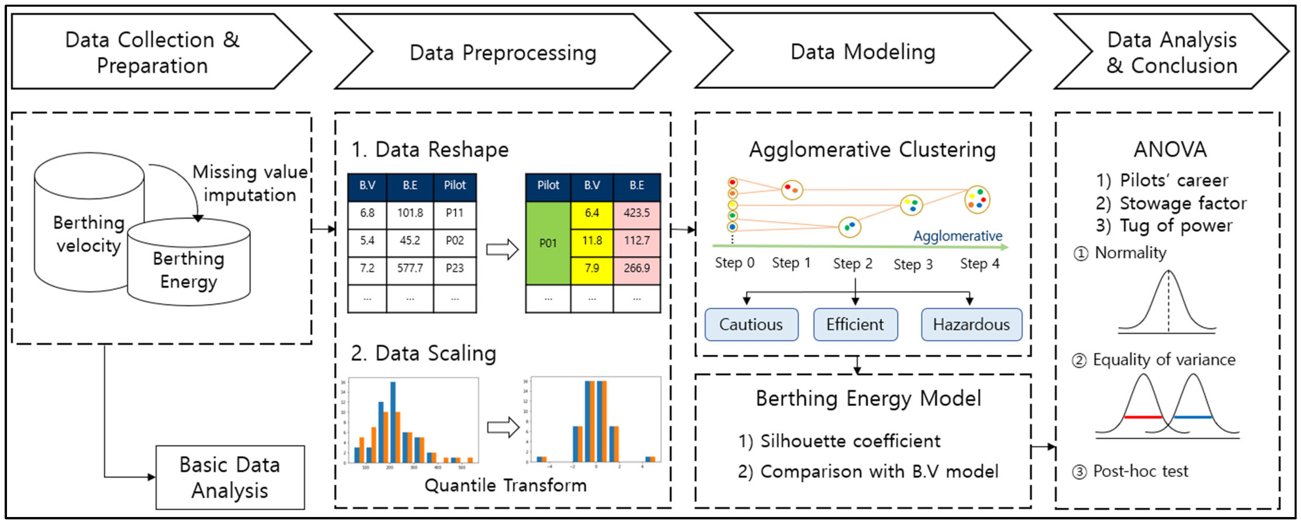
Figure 1 shows the overall study flow. First, berthing velocity data were collected, and berthing energy was calculated by filling in missing values. The basic data analysis was performed separately for the berthing velocity, and berthing velocity and berthing energy data were preprocessed through reshaping and scaling. Pilots were grouped using an agglomerative clustering algorithm, and the final cluster model was determined by comparing the silhouette coefficients and analysis results. Finally, analysis of variance (ANOVA) and post hoc tests were performed to assess the differences among groups.

2.1. Analysis Variables

2.1.1. Berthing Energy

During berthing, the amount of impact generated by contact with facilities, such as fenders, is called the berthing energy, which is used to select the pier fenders. Fenders are often used to absorb berthing energy to reduce the impact of a berthing ship [23]. According to harbor and fishery design criteria, the method to obtain the berthing energy of a ship uses the following kinematic equation [24]:

$$E_f=\left(\frac{M_s{V}^2}{2}\right)C_e{C}_m{C}_s{C}_c$$

(1)

when a ship moves horizontally and berths, kinetic energy is generated by the ship; accordingly, $M_s \left(tonnes\right)$ denotes the ship mass, and $V \left(cm/s\right)$ denotes the berthing velocity. Equation (1), which is an equation for calculating the berthing energy $E_f \left(kN·m\right)$, is constructed considering the energy absorbed by the fender, i.e., the eccentricity factor $C_e$, the virtual mass factor $C_m$, the softness factor $C_s$ (standard is 1.0), and the berth configuration factor $C_c$ (standard is 1.0).

The eccentricity factor $C_e$ considers the energy loss due to rotation caused by the berthing ship not coming in parallel with the berth and a part of the hull coming into contact with the mooring facility first. The virtual mass factor $C_m$ indicates that the inertial force due to the seawater mass is added to the ship due to the hull acceleration. The softness factor $C_s$ represents the energy absorbed by the deformation of the ship’s shell. The configuration factor of the berth $C_c$ is a buffering effect that occurs due to the compression of seawater between the ship and mooring facilities, indicating a decrease in energy absorbed by the fender [25]. Therefore, the berthing energy is calculated based on the largest ship, and the fender with energy capable of absorbing the berthing energy is finally selected. 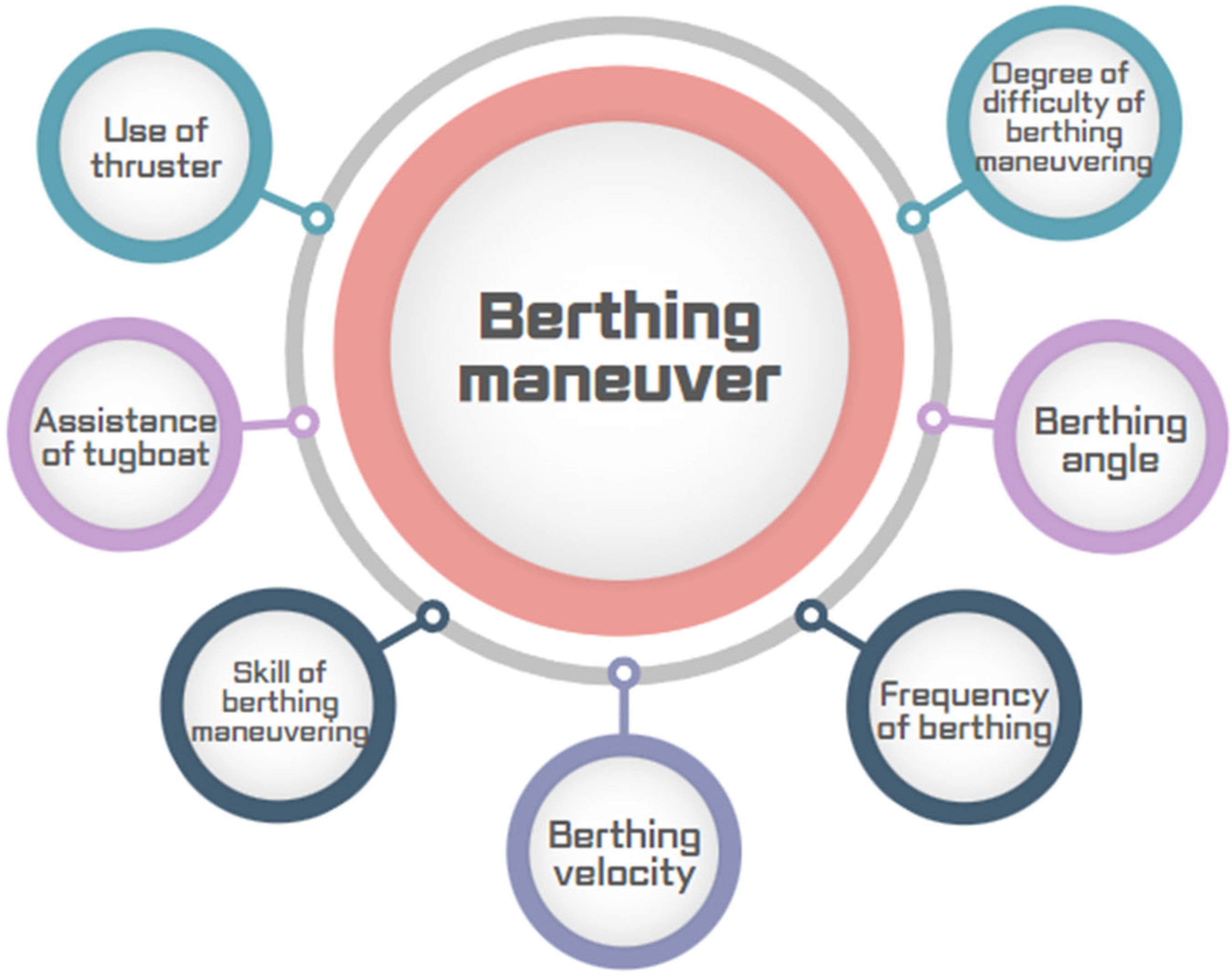Figure 2 depicts an excerpt of components to consider when designing a fender [12]. Among the various factors, the berthing maneuver part, which is probably related to this study, was focused on. In particular, the skill of berthing maneuvering and berthing frequency are closely related to the pilot’s ability and career.

2.1.2. Berthing Velocity

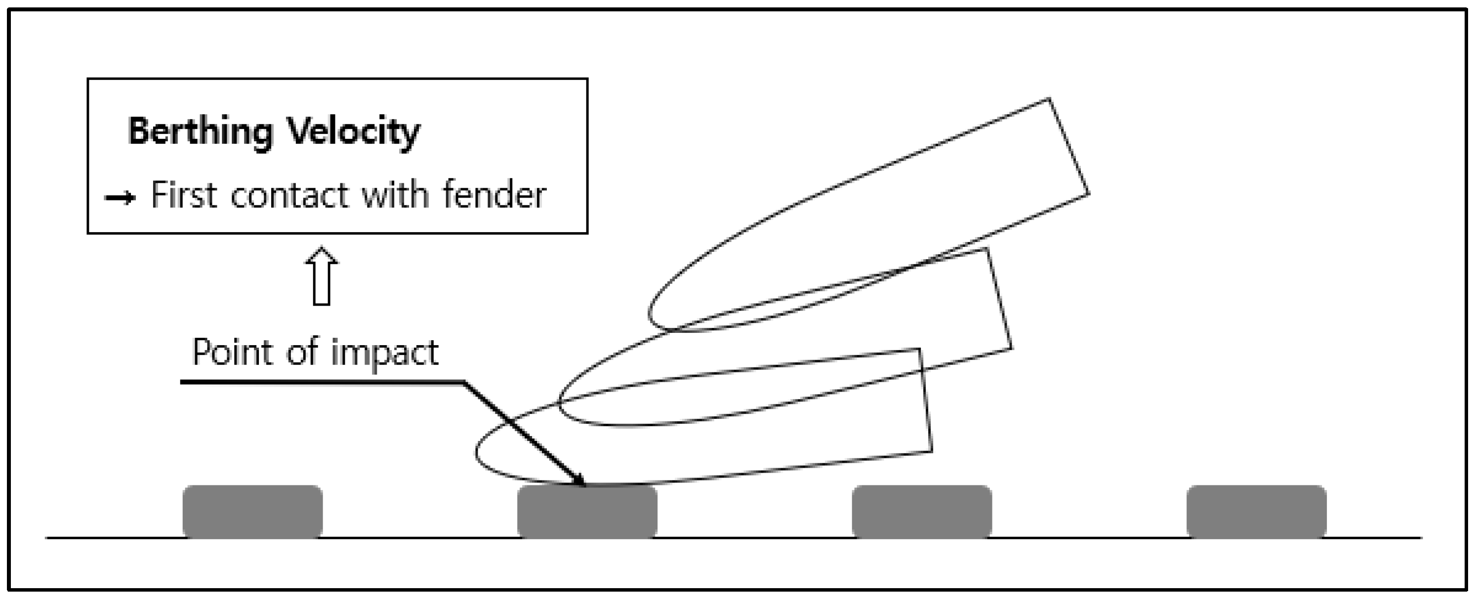
As shown in Figure 3, the berthing velocity is measured vertically at the time of first contact with the pier. A ship’s berthing energy is most influenced by the berthing velocity; in fact, a ship’s berthing energy is proportional to the square of the berthing velocity.

To date, the design codes and standards for fender design still rely on a deterministic design approach in which the overall factors of safety are applied to the berthing energy. However, this design approach does not explicitly account for the uncertainty in design parameters and does not consider the failure probability of the fender system, i.e., the probability that the actual berthing energy exceeds the design value. Berthing velocity is the major source of uncertainty in berthing energy. Therefore, the berthing policy within a port significantly influences the berthing velocity at the moment of impact.

2.2. Data Collection

The data collection target pier is an tanker terminal located in Yeosu equipped with a docking aid system (DAS) for measuring berthing velocity, and 915 data points were collected for about five years from March 2017 to February 2022. Berthing velocity data are unique and valuable; besides, considering the PIANC Working Group 145 report, it is rare that only about 2300 berthing velocity data points can be collected from 14 different berths located in seven countries. We increased the data reliability by targeting the data accumulated over a long period in one berth.

2.2.1. DAS

DAS mainly comprises a laser-type measurement system and display software that enables real-time berthing control to be monitored. At the target pier, two lasers that detect ships from a distance of 2–300 m are installed on each jetty (Figure 4a). The lasers feature eye-safe, waterproof, and specially coated glass. The measuring range of the laser is up to 300 m, the measuring accuracy is ± 2.5 cm, and the sampling rate is 2 KHz. The distance between the lasers enables the DAS to calculate the ship angle and distance to the fenders. A pair of lasers placed at a known distance apart measure the distance from the berthing line to the ship hull forward and aft. The change in range over time is employed to calculate the approach velocity perpendicular to the berthing line relative to the two laser locations. Simple geometry is used to calculate the berthing angle. The distance, speed, and angle are shown on a digital large display (DLD) (Figure 4b). The DLD shows distance with a decimal point and has features such as illumination for night approach and visibility up to 250 m away. The DLD shows distance, speed, acceleration/deacceleration, and warning due to excessive speed. In the control room, live data are displayed and stored on a computer (Figure 4c).

2.2.2. Data Collection Target Pier

The tanker terminal is divided into three jetties: Jetties 1–3 (Figure 5). It is a closed jetty and is a protected harbor where mountains and islands act as natural breakwaters, so the influence of waves and currents is minimal.

Table 1. Terminal specifications.

	Jetty 1	Jetty 2	Jetty 3
Capacity (DWT)	80,000	120,000	320,000
Maximum length overall (M)	295	321	382
Water Depth (M)	17.0	18.0	19.5
Maximum Draft (M)	14.7	15.5	17.7
Berthing Velocity (designed; cm/s)	12	15	15
Berthing Velocity (operated; cm/s)	safety: 5, warning: 6–10, dangerous: 11–15

shows the terminal specifications: berthing capacity for each pier, maximum length overall, maximum draft, water depth, designed berthing velocity, and operated berthing velocity.

The berth depth standard is determined based on the sum of the excess water depth corresponding to the maximum draft, such as the full load draft of the target ship, so it can estimate the berthing ship size by assessing the water depth [24]. The water depth of Yeosu Gwangyang Port where the target pier exists is distributed as shown in Figure 6.

2.3. Data Preprocessing

Data directly taken from the source will likely have inconsistencies and errors, and most importantly, they are not ready to be used for a data analysis process [26]. In addition, depending on the data characteristics and results to be analyzed, suitable tools are required. It is possible to convert the impossible to possible, adapting data to fulfill the input demands of each data mining algorithm. In the process of data collection, the values with abnormal berthing velocity were determined as outliers and removed. The data preprocessing used in this study includes the missing value imputation, data reshaping, and data scaling.

2.3.1. Missing Value Imputation

Missing value imputation is a basic solution method for incomplete dataset problems, particularly those where some data samples contain one or more missing attribute values [27]. In this study, missing values are replaced with imputed values from a particular technique, such as the median value. Based on the complete dataset with missing value imputation in

Table 2. The amount of missing values.

Variables	Non-Null Count	Missing Value Ratio	Data Type
DWT	915	0%	float
Berthing Velocity	915	0%	float
Draft	898	1.86%	float
Length between perpendiculars	915	0%	float
Breadth	915	0%	float
Pilot	915	0%	object

, the berthing energy can be calculated.

2.3.2. Data Reshaping

Data reshaping is a common task in data analysis. It involves the rearrangement of the form of data, but not the content. Reshaping is similar to creating a contingency table, as there are many strategies to arrange the same data, but it differs in that there is no aggregation [28].

To group the maneuvering types of pilots based on berthing velocity and berthing energy, it is imperative to reshape our data to have each analysis value for each pilot. The average and standard deviation values of the variables for each pilot were used for analysis.

2.3.3. Data Scaling

Data scaling and data normalization aim to consolidate or transfer data into ranges and forms appropriate for modeling. In general, models trained on scaled data significantly outperform those trained on unscaled data; therefore, data scaling is an essential step in data preprocessing. In the berthing energy data of the present study, the silhouette coefficient is 0.4425 without scaling, which is low compared to the results in Table 5. Data scaling is particularly crucial for methods that use distance measures, such as nearest neighbor classification and clustering [29].

In this study, we employed a quantile transformation method as the data scaling method. It is possible to use a quantile transformer that uses information contained in a quantile to make data uniformly or normally distributed [30]. Smoothing the original distribution has the disadvantage of distorting correlations and distances within and across features but has the advantage of making it easy to compare characteristics measured at different scales. The quantile transformer formula is expressed as follows (2):

$$G^{-1}\left(F\left(x\right)\right)$$

(2)

where $F$ denotes the cumulative distribution function (CDF) of $x$ and $G^{-1}$ denotes the quantile function of output distribution $G$.

The quantile function, also known as the percentage point function (PPF), is the inverse of the CDF. A CDF is a function that returns the probability of a value at or below a given value, and PPF is a function that returns the value at or below a given probability.

2.4. Agglomerative Clustering

Clustering algorithms are mainly categorized into hierarchical clustering, partitioning, density-based clustering, grid-based clustering, model-based clustering, and fuzzy clustering [31]. Hierarchical agglomerative clustering is a well-established algorithm in unsupervised ML. The agglomerative clustering approach starts by splitting a dataset into singleton nodes and gradually merging current pairs closest to each other into new nodes until one final node makes up the entire dataset [32].

Various clustering schemes share this procedure as a common definition but differ in how the measure of dissimilarity between clusters is updated after each step. In this study, the ward linkage method is employed.

Agglomerative clustering works from the dissimilarities between the dataset to be grouped together. A type of dissimilarity can be suited to the subject and the nature of the data, and one of the results is a dendrogram showing the progressive grouping of the data. It can be used to gain a suitable number of classes into which the data can be grouped. As it does not start from a random point, the result does not change every time.

2.4.1. Ward Linkage

The types of inter-cluster linkages in agglomerative clusters include single, complete, average, centroid, and ward linkages. All other linkages except ward linkages are methods of forming clusters based on the Euclidean squared distance. On the other hand, the ward is the only method based on a classical sum-of-squares (SS) criterion to generate groups that minimize the within-group variation at each binary fusion [33].

Let the number of samples be $n$, the number of clustered groups be $k$, the $i$-th sample of cluster $G_t$ be $X_i^{\left(t\right)}$, the number of samples in $G_t$ be $n_t$, and the cluster center be ${\overline{X}}^{\left(t\right)}$. The SS within a group is expressed as follows:

$$S_t={\displaystyle \sum }_{i=1}^{n_t}{\left(X_i^{\left(t\right)}-{\overline{X}}^{\left(t\right)}\right)}^T\left(X_i^{\left(t\right)}-{\overline{X}}^{\left(t\right)}\right)$$

(3)

The total SS for k groups is expressed as follows:

$$S={\displaystyle \sum }_{t=1}^k{S}_t={\displaystyle \sum }_{t=1}^k{\displaystyle \sum }_{i=1}^{n_t}{\left(X_i^{\left(t\right)}-{\overline{X}}^{\left(t\right)}\right)}^T\left(X_i^{\left(t\right)}-{\overline{X}}^{\left(t\right)}\right)$$

(4)

Assume that $G_p$ and $G_q$ each denote a cluster. The distance between $G_p$ and $G_q$ is defined as the SS between the two clusters:

$$D^2\left(G_p,G_q\right)=S_r-S_p-S_q$$

(5)

This study used the ward linkage, which is less sensitive to noise and has a strong tendency to generate clusters of similar size.

2.4.2. Euclidean Distance

In general, the distance definition refers to the Euclidean distance and represents the actual distance between two points in an m-dimensional space or the natural length of a vector [34]. In this study, we assumed that the input point is given as a vector in the Euclidean space in the formula of the ward method and used the Euclidean distance:

$$d\left(x_i,x_j\right)=\sqrt{{\displaystyle \sum }_{k=1}^m{\left(x_{ki}-x_{kj}\right)}^2}$$

(6)

2.5. Silhouette Coefficient

The silhouette coefficient has a value from −1 to 1. The closer the silhouette coefficient is to 1, the better the clustering. In this study, we use the intrinsic silhouette coefficient to select a better variable by comparison.

$$\mathrm{S}\left(i\right)=\frac{b\left(i\right)-a\left(i\right)}{\max \left(a\left(i\right),b\left(i\right)\right)}$$

(7)

where $a\left(i\right)$ denotes the density within the cluster containing object $i$, and $b\left(i\right)$ denotes how far off object $i$ is from other clusters [35].

3. Results

3.1. Basic Data Analysis

To determine the status of berthing velocity by jetty, a basic statistical analysis was performed; the results of analyzing the berthing velocity characteristic values are shown in

Table 3. Characteristics of the berthing velocity values by jetty.

Velocity (cm/s)	Jetty 1	Jetty 2	Jetty 3	Total
Mean (cm/s)	7.01	8.43	6.90	7.48
Standard Deviation (cm/s)	3.27	4.04	2.86	3.54
Coefficient of Variance	0.47	0.48	0.41	0.47
Maximum Observed Value (cm/s)	19.98	21.21	18.41	21.21
Number of Data Points	376	320	219	915

. The mean value and standard deviation of all 915 data points are 7.48 and 3.54 cm/s, respectively. Although some ships exceeded the operated dangerous velocity in all jetties, the ships berthing at the pier were generally berthing at a safe berthing velocity.

Table 4. Frequency of berthing velocity.

Velocity (cm/s)	Count	Cumulative Count	Relative Frequency (%)	Cumulative Frequency (%)
0–2	21	21	2.3	2.3
2–4	88	109	9.6	11.9
4–6	238	347	26.0	37.9
6–8	238	585	26.0	63.9
8–10	151	736	16.5	80.4
10–12	86	822	9.4	89.8
12–14	41	863	4.5	94.3
14–16	22	885	2.4	96.7
16–18	14	899	1.5	98.3
18−20	13	912	1.4	99.7
20	3	915	0.3	100.0

analyzes the frequency and relative frequency of each berthing velocity for the total berthing velocity. The berthing velocity is subdivided further, and the berthing velocity values of 4–6 and 6–8 cm/s account for 26% each, which is the highest frequency. The berthing velocity within 10 cm/s accounts for 80.4%, and that exceeding the limit of 15 cm/s at the pier is less than 5%. It can also be confirmed from the frequency analysis that the berthing velocity of ships berthing at the target pier is generally not high.

The relationship between the ship size (DWT) and berthing velocity is visualized as a scatter plot (Figure 7a). Nondimensionalization was performed to check the size of ships berthing compared with the berthing capacity of each jetty. Nondimensionalization means that the dimension is removed, and because the unit disappears, size comparison is easy [36]. If the berthed ship size for each jetty is divided by the designed berthing capacity of the pier, the dimensionless result of the ship size is derived. Figure 7b–d show the graph of the relationship between the dimensionless results and berthing velocity. For Jetty 1, most ships with a size corresponding to about 0.5–0.7 compared with the berthing capacity were berthed. For Jetty 2, ships of various sizes within the berthing capacity range were berthed, and for Jetty 3, ships with sizes of 0.5 or less were berthed, except for ships of a size similar to the berthing capacity. Ships of various sizes berth at different berthing velocities. Therefore, in this study, in addition to the berthing velocity, we consider the berthing energy, which is a calculated value based on the ship size, as another analysis variable.

Figure 8 visualizes the berthing energy and velocity for each pilot in a boxplot. The mean and standard deviation values of the berthing energy and velocity are expressed in the order of pilot ID. The boxplot is standard for displaying the data distribution based on the minimum, first quartile, median, third quartile, and maximum in the dataset. It displays the data range and distribution along a number line. Although there is a disadvantage that the original data are not clearly shown in a boxplot, this was resolved by displaying the scatter on the boxplot. For standard deviation, we display a violin plot that expresses the data shape by overwriting the kernel density curve symmetrically on the boxplot to make it easy to visualize the degree of deviation.

In this study, we group the maneuvering types of pilot using a clustering algorithm based on the mean and standard deviation of the berthing energy and velocity data reshaped for each pilot. Before cluster analysis, which is a parametric statistical analysis method, data normality was checked using a parametric method (Figure 9). The Kolmogorov–Smirnov (K–S) test was employed for the normality test. As a result (

Table 5. Results of the Normality test.

K–S test		Normal
		p-Value	Result
Berthing Energy	Mean	0.3585	adopt
	Std	0.4658	adopt
Berthing Velocity	Mean	0.9136	adopt
	Std	0.6461	adopt

), the p-value exceeded 0.05 and followed normality in all cases.

3.2. Clustering of Pilots’ Maneuvering Type

3.2.1. Results by Variables

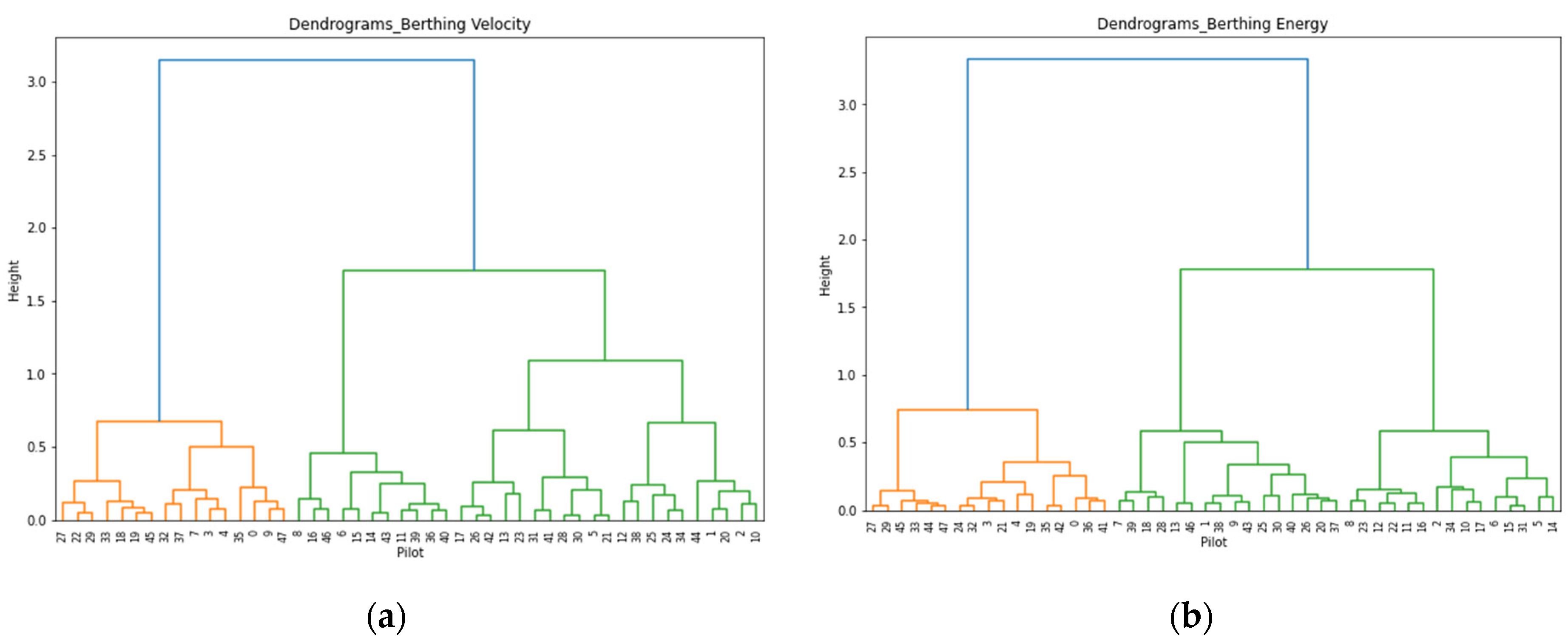
After the agglomerative clustering was applied to the mean and standard deviation values of the preprocessed berthing velocity and energy data, the results shown in Figure 10 were derived. A dendrogram shows the order in which objects are combined in a tree-like structure, and the final grouping can be determined through cutting. Usually, cutting is performed at the level where the distance between the clusters is the most distant; according to Figure 10, the variables of this study are finally grouped into three clusters.

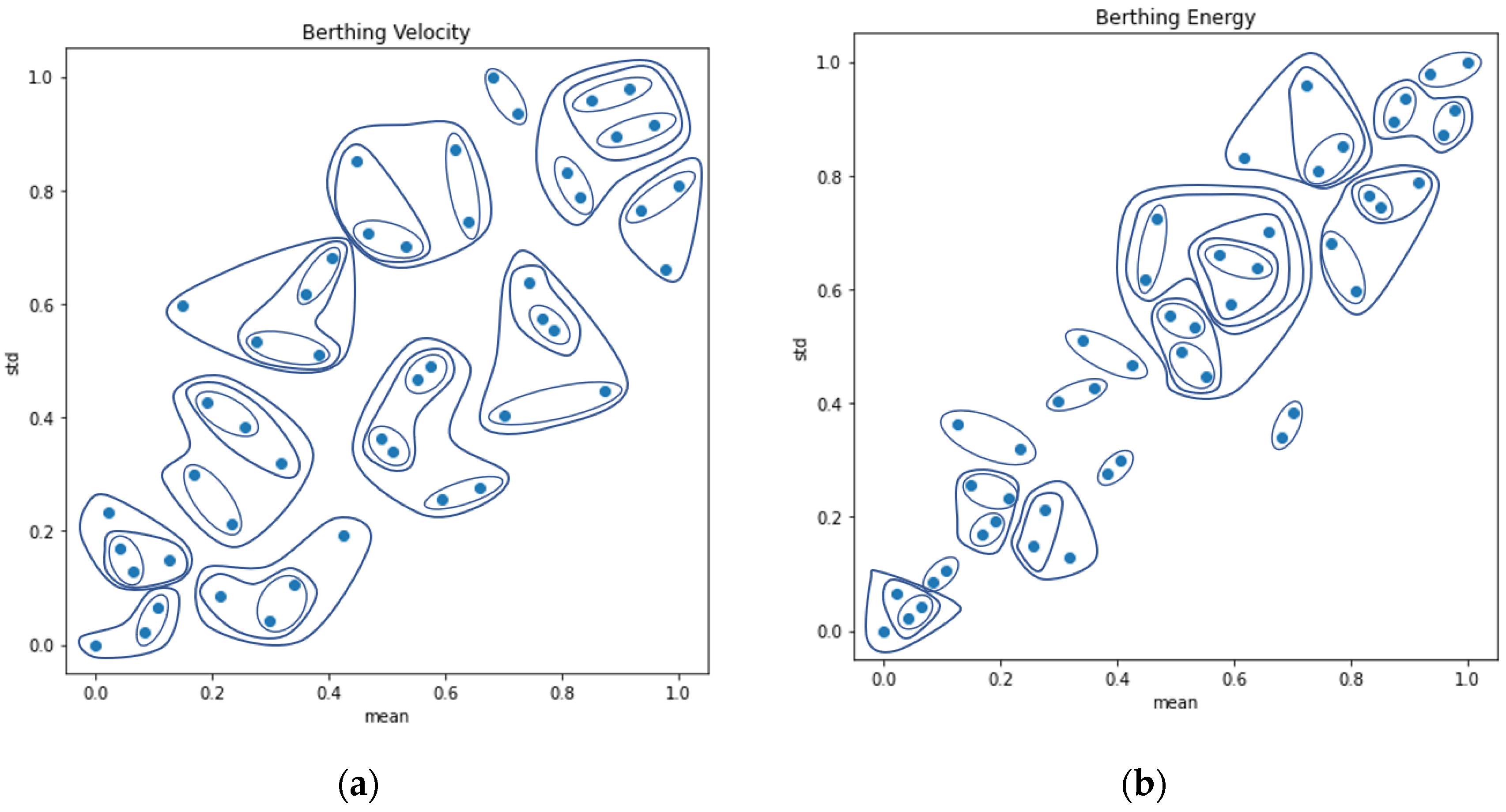
Figure 11a–d show scatter graphs of the mean and standard deviation of the berthing velocity and berthing energy after preprocessing. Figure 11a,b visualize each cluster stage according to a dendrogram; each data point is regarded as one cluster, and three clusters are finally created by connecting close clusters. Figure 11c,d are graphs visualized so that the final three clusters can be recognized at a glance. The three pilot types clustered according to the mean and standard deviation were defined as cautious, efficient, and hazardous types. If the mean of the berthing velocity/energy is low and the standard deviation is small, it is judged that berthing with a safe berthing velocity is constant, and it is sorted as a cautious type. If the mean of the berthing velocity/energy is high and the standard deviation is large, it is judged that berthing with a dangerous berthing velocity is not constant, and it is sorted as a hazardous type. The types with the mean and standard deviation in between were judged differently depending on the situation of the berthing velocity, which is neither safe nor dangerous, and is sorted as the efficient type.

In this study, two methods were used and compared to evaluate the model with higher performance between the berthing velocity and energy. First, we evaluated the performance using the well-known silhouette analysis as a clustering evaluation technique. As a result, the silhouette analysis showed high performance for the berthing energy and velocity at the silhouette coefficients of 0.5133 and 0.4163, respectively (

Table 6. Silhouette coefficients.

	Silhouette Coefficient	Result
Berthing velocity	0.4163
Berthing energy	0.5133	√

).

Another technique was to compare the clustering results of the berthing velocity and energy.

Table 7. Pilots’ movement according to each variable.

	Cautious (Constant Low Speed)			Efficient (More or Less Constant Moderate Speed)			Hazardous (Unstable High Speed)
Berthing Velocity	$16(C_v{C}_e+C_v{E}_e+C_v{H}_e$)			$21(E_v{C}_e+E_v{E}_e+E_v{H}_e$)			$11(H_v{C}_e+H_v{E}_e+H_v{H}_e$)
↓	$C_v\to C_e$$\left(C_v{C}_e\right)$	$C_v\to E_e$$\left(C_v{E}_e\right)$	$C_v\to H_e$$\left(C_v{H}_e\right)$	$E_v\to C_e$$\left(E_v{C}_e\right)$	$E_v\to E_e$$\left(E_v{E}_e\right)$	$E_v\to H_e$$\left(E_v{H}_e\right)$	$H_v\to C_e$$\left(H_v{C}_e\right)$	$H_v\to E_e$$\left(H_v{E}_e\right)$	$H_v\to H_e$$\left(H_v{H}_e\right)$
	11	4	1	5	8	8	1	4	6
Berthing Energy	$17(C_v{C}_e+E_v{C}_e+H_v{C}_e$)			$16(C_v{E}_e+E_v{E}_e+H_v{E}_e$)			$15(C_v{H}_e+E_v{H}_e+H_v{H}_e$)

shows the number of pilots who moved by type based on the clustering results of the berthing velocity and energy. The sums of $X_{v}Y\left(X=C,E,H\right)$ and $X{Y}_e\left(Y=C,E,H\right)$ for each type is the sums of pilots clustered with berthing velocity and energy, respectively. Although there are pilots of the same type that do not change, there is a shift from one type to another in all cases. In particular, switching from the cautious to hazardous type or vice versa indicates that the berthing energy was high or low, whereas the berthing velocity was low or high, respectively. This was significantly influenced by the ship size. Therefore, it was judged that it is correct to group pilots based on the berthing energy that considers several factors, not just the berthing velocity, and the case where the berthing energy is a variable was selected as the final model.

3.2.2. Cluster-Specific Characteristics

Based on the final selected model, we investigated the characteristics of each cluster. Whether there was a difference in the pilots’ career, stowage factor, and the tug of power was assessed using one-way ANOVA. The careers of pilots listed in the Yeosu Pilot Society were referred to, and the stowage factor was calculated by dividing the capacity tonnage by each ship’s DWT. The tug of power is the sum of the horsepower of the tugs used at berthing for each vessel. The normality of the distribution of all samples was assessed using the Shapiro–Wilk (S–W) test. As shown in

Table 8. Normality test of variance.

	Type	S–W Statistic	p-Value
Pilots’ career	Cautious	0.8856	0.0393
	Efficient	0.9255	0.2065
	Hazardous	0.8444	0.0145
Stowage factor	Cautious	0.9330	0.2446
	Efficient	0.9689	0.8199
	Hazardous	0.9421	0.4096
Tug of power	Cautious	0.9018	0.0727
	Efficient	0.9199	0.1678
	Hazardous	0.9069	0.1213

, for the pilots’ career, the p-value did not exceed 0.05 in the cautious and hazardous types, so we could confirm that normality did not follow the alternative hypothesis.

Therefore, the Kruskal–Wallis H test, a nonparametric test, was performed, and the p-value was 0.0121, which did not exceed the significance level of 0.05, confirming that there was a statistically significant difference (

Table 9. Nonparametric test.

	Kruskal–Wallis H Statistics	p-Value
Pilots’ career	8.8368	0.0121

).

Using Levene’s test, the pairwise comparisons of two variables following normality were assessed under the assumption of the equality of variance. As shown in

Table 10. Levene’s test.

	Levene Statistic	p-Value
Stowage factor	1.4780	0.2389
Tug of power	0.2492	0.7805

, the test results confirmed that the p-values of both variables exceeded the significance level and were equally distributed according to the null hypothesis.

Subsequently, as a result of ANOVA, the significance probability was 0.05 or less, indicating a difference in the mean between groups under the significance level (

Table 11. Results of ANOVA.

	df	Sum_sq	Mean_sq	F	PR(>F)
Stowage factor	2	0.0525	0.0263	3.2562	0.0478
Tug horse power	2	4.3290e+07	2.1645e+07	10.8637	0.0001

).

A post hoc test is usually performed to reveal specific differences between three or more group means when the ANOVA test is found to be significant [37]. Bonferroni correction with the Mann–Whitney U test was performed as a post hoc test by Kruskal–Wallis H. The correction is the procedure of adjusting the significance level of a statistical test to avoid a type I error when multiple comparisons are made. As shown in

Table 12. Results of the post hoc test.

	Group 1	Group 2	Meandiff 1	p-Value	Reject	Type
Pilots’ career	Cautious	Efficient	0.8971	1.0	False	Bonferroni Mann–Whitney U
	Cautious	Hazardous	5.5137	0.0211	True
	Efficient	Hazardous	−4.6167	0.0541	False
Stowage Factor	Cautious	Efficient	0.0430	0.3963	False	Scheffe
	Cautious	Hazardous	0.0810	0.0485	True
	Efficient	Hazardous	−0.0380	0.5057	False
Tug of power	Cautious	Efficient	269.25	0.8612	False	Scheffe
	Cautious	Hazardous	2165.22	0.0004	True
	Efficient	Hazardous	−1895.97	0.0023	True

¹ (mean of Group 2) − (mean of Group 1)

, there was a significant difference between the cautious and hazardous types. Two variables that met the assumption of ANOVA through parametric testing were post-tested using Scheffe’s method, the most conservative multicomparison test [38]. Scheffe’s post hoc test showed that there were statistically significant differences (p < 0.05) between the various types (particularly cautious and hazardous) for the stowage factor and tug of power.

4. Discussion

In this study, we aimed to group the maneuvering types of pilots through berthing velocity data, which are difficult to visualize and collect. To emphasize the relevance of the berthing velocity data, basic data analysis was performed to determine the berthing velocity characteristics and distribution. In particular, through the nondimensionalization result, it can be confirmed that ships of various sizes for each jetty berth at the pier, and most of them exist within the berthing capacity category. However, even at the same berthing velocity, the energy impact significantly differed depending on the ship size, so it was judged that there is a limit to sorting the degree of risk with only the berthing velocity data. Therefore, we evaluated the berthing energy that can simultaneously consider the effects of the ship size and berthing velocity and used it as basic data in the same manner as the berthing velocity. Through preprocessing, each pilot was arranged to have scaled berthing velocity and energy data, and the mean and standard deviation were used for analysis. The mean and standard deviation of each data can be used as variables because the degree of risk of the berthing velocity can be determined through the mean and whether the trend of the berthing velocity is constant can be assessed through the standard deviation. As a result of agglomerative clustering, we finally realized three clusters, which we grouped as cautious, efficient, and hazardous types. Pilots who berth at a constant low-berthing velocity were judged to berth safely and were sorted as the cautious type. As this is the safest type of piloting, it may be considered the most desirable, but it is not necessarily the case. Given that the pilots are careful in all situations, there is a disadvantage that it may take a long time to pilot. Pilots who have a higher standard deviation than the cautious type at normal berthing velocity but who berth more or less uniformly were sorted as the efficient type. This study judged that this is an efficient type of berthing under appropriate judgment in various situations rather than being cautious every time. Pilots who berth irregularly with a relatively high berthing velocity are sorted as hazardous, and they definitely need to berth more safely. The maneuvering type was also grouped by the berthing energy, and as a result of synthesizing the silhouette coefficient and type movement between the two, it was judged that it was accurate to determine the model using the berthing energy as a variable. These are all data-based grouping results of maneuvering types, and it is not a matter of deciding which type is more appropriate and desirable.

This study has great significance in quantitatively grouping maneuvering types of pilots based on data. Its novelty is that the berthing energy is used as basic data and another clustering algorithm based on distance called the agglomerative clustering algorithm is used. Compared with the k-means algorithm, the agglomerative clustering algorithm has the advantages of being able to check an entire cluster through a dendrogram and using it without setting the number of clusters. In addition, a new result was realized using the berthing energy as a variable. We also evaluated whether there was a significant difference according to the cluster by designating the factors affecting the berthing energy as variables. Consequently, we confirmed that there was a significant difference between the cautious and hazardous types in all variables. In the hazardous type rather than the cautious type, the pilots have more experience, the tonnage is large, and the horsepower of the tug is large. Through this, pilots tend to become bolder as they build up their careers, and the greater the horsepower of the tug and the greater the tonnage, the more difficult it is to maneuver.

In this study, we grouped the maneuvering types of pilots based on the berthing velocity data, but there were limitations. Because berthing velocity only refers to the speed at the time of contact and cannot be said to contain the overall flow of the berthing process, it is unsuitable for grouping the maneuvering types of pilot. If the trajectory data containing the berthing process of the ship are used, more reliable results can be derived, and it is expected that the usage of the berthing velocity data will also increase.

5. Conclusions

In this study, the berthing energy was calculated based on the collected berthing velocity data and used as the basic data of the study together with the berthing velocity data. As a result of basic data analysis, we confirmed that the berthing velocity of ships berthing at the target pier was not generally high, existing within the berthing capability category, and the analysis variables followed a normal distribution. Preprocessing was performed through data reshaping and scaling, and pilot types were grouped into three (cautious, efficient, and hazardous) using the agglomerative clustering algorithm. The final cluster model using the berthing energy was determined through a comparison of the silhouette coefficient and analysis results. Finally, ANOVA and post hoc tests were performed to confirm that there was a significant difference, particularly in the cautious and hazardous types.

The Korean pilot society, through the pilot assignment guidelines, stipulates the permission of two or more pilots with different pilot licenses and the relationship between the pilots [39]. To ensure the safety of ship operation, the Yeosu Port Pilot Society allows two or more pilots to board and pilot the ship simultaneously in the case of piloting a large ship of 30,000 gross tonnage or more or a special ship. It stipulates that two or more pilots must be on board for ships loaded with dangerous goods, such as oil tankers, liquid natural gas, and liquid petroleum gas carriers. At this time, the roles of the lead pilot and copilot are divided, and the copilot usually performs auxiliary tasks, such as checking whether the tug boat is acting according to the lead pilot’s command, the waterway status, the wharf status, the incoming and outgoing ships, and contact information with other ships [40]. In this study, we grouped the maneuvering types of pilots into three (cautious, efficient, and hazardous) using the berthing energy cluster model. Based on this study, if different types of pilots are assigned as the lead pilot and copilot, it is possible to create a pilot environment that exploits each other’s strengths and weaknesses, rather than just performing auxiliary tasks. In addition, while piloting, there are many times when joint piloting is required, and there are many situations where pilots encounter other ships. Therefore, understanding the abilities and tendencies of each pilot in advance can be advantageous.

In addition, this study can provide basic data in the safety management part. If an accident occurs during the pilot ship’s maneuvering, the captain, the owner’s agent, becomes responsible for the operation, and the terminal or shipper will be held responsible for the shipping company. In such a situation, it is the position of the shipowner or supervisor that by requiring the pilot to comply with the berthing velocity or the type of maneuvering based on our results, the burden on the shipping company can be lessened while still emphasizing the risks to the pilots.

References

- Ji, S.W. A study on the license system for pilot in Japan. Marit. Law Rev. 2012, 24, 11. [Google Scholar]
- Go, J.H.; Kim, H.D. An effect of organizational justice and organizational support of the pilots’ association on job satisfaction and job commitment of the pilot. J. Shipp. Logist. 2017, 33, 29–56. [Google Scholar]
- Hsu, W.K.K. Assessing the safety factors of ship berthing operations. J. Navig. 2015, 68, 576–588. [Google Scholar] [CrossRef] [Green Version]
- Orlandi, L.; Brooks, B. Measuring mental workload and physiological reactions in marine pilots: Building bridges towards redlines of performance. Appl. Ergon. 2018, 69, 74–92. [Google Scholar] [CrossRef] [PubMed]
- Ohasni, N.; Sugihara, Y. Mental tension of ship operators I: Mental tension at the time of departure and arrival of large ship. J. Jpn. Voyag. Soc. 1967, 38, 31–38. [Google Scholar]
- Fukuchi, N. Occurrence of ship accidents based on tension stress and measures to support navigation. J. Soc. Instrum. Control Eng. 2006, 45, 689–694. [Google Scholar]
- Khan, Q.A.; Hassan, A.; Rehman, S.; Riaz, F. Detection and classification of pilots cognitive state using EEG. In Proceedings of the IEEE International Conference on Computational Intelligence and Applications (ICCIA), Beijing, China, 8–11 September 2017; pp. 407–410. [Google Scholar]
- Lee, D.H.; Jeong, J.H.; Kim, K.D.; Yu, B.W.; Lee, S.W. Continuous EEG decoding of pilots’ mental states using multiple feature block-based convolutional neural network. IEEE Access 2020, 8, 121929–121941. [Google Scholar] [CrossRef]
- Foreign Captain ‘Shush’ Arrested after Ship Accident… 10 Billion Won Damage. Available online: https://news.sbs.co.kr/news/endPage.do?news_id=N1006741341&plink=LINK&cooper=YOUTUBE&plink=COPYPASTE&cooper=SBSNEWSEND (accessed on 7 May 2022).
- Marine Safety Investigation Team (Korea Maritime Safety Tribunal, Sejong, Republic of Korea). Marine Safety Investigation Report on M/V MILANO BRIDGE–Contact with Gantry Cranes–, 12 January 2021; [MSI Report 2021-001]; Marine Safety Investigation Team: Sejong, Korea, 2021. [Google Scholar]
- Marine Casualty Investigation Team (Korean Maritime Safety Tribunal, Sejong, Republic of Korea). Investigation Report of Very Large Crude Oil Tanker Wu Yi San’s Contact with Dolphins, 9 January 2015; Marine Safety Investigation Team: Sejong, Korea, 2015. [Google Scholar]
- Maritime Navigation Commission (The World Association for Waterborne Transport Infrastructure, PIANC). Berthing Velocity Analysis of Seagoing Vessels Over 30,000 DWT; Maritime Navigation Commission: Seoul, Korea, 2020. [Google Scholar]
- Brolsma, J.U. On fender design and berthing velocities. In Proceedings of the International Navigation Congress, Leningrad, Russia, 28 August 1977; pp. 87–100. [Google Scholar]
- Roubous, A.; Groeneween, L.; Peters, D.J. Berthing velocity of large seagoing vessels in the port of Rotterdam. Mar. Struct. 2017, 51, 202–219. [Google Scholar] [CrossRef]
- Cho, I.S.; Cho, J.W.; Lee, S.W. A basic study on the measured data analysis of berthing velocity of ships. J. Coast. Disaster Prev. 2018, 5, 61–71. [Google Scholar] [CrossRef]
- Iversen, R.; Argo, M.L.; Cortes, S.C.; Pyun, J.J. Analysis of measured marine oil terminal berthing velocities. In Ports 2019: Port Planning and Development; American Society of Civil Engineers: Reston, VA, USA, 2019; pp. 162–172. [Google Scholar]
- Lee, H.T.; Lee, S.W.; Cho, J.W.; Cho, I.S. Analysis of feature importance of ship’s berthing velocity using classification algorithms of machine learning. J. Korean Soc. Mar. Environ. Saf. 2020, 26, 139–148. [Google Scholar] [CrossRef]
- Lee, H.T.; Lee, J.S.; Son, W.J.; Cho, I.S. Development of machine learning strategy for predicting the risk range of ship’s berthing velocity. J. Mar. Sci. Eng. 2020, 8, 376. [Google Scholar] [CrossRef]
- Kang, E.J.; Lee, H.T.; Cho, I.S. Analysis of allowable berthing velocity by ship size considering designed energy. J. Coast. Disaster Prev. 2021, 8, 297–306. [Google Scholar] [CrossRef]
- Inoue, K. Guidelines for desirable berthing operation. J. Jpn. Inst. Navig. 1990, 82, 43–52. [Google Scholar]
- Ishihata, S. Actual berthing speed of VLCC and its optimum speed. J. Jpn. Inst. Navig. 1988, 79, 177–184. [Google Scholar] [CrossRef] [Green Version]
- Lee, H.T.; Lee, J.S.; Cho, J.W.; Yang, H.; Cho, I.S. A study on the pattern of pilot’s maneuvering using k-means clustering of ship’s berthing velocity. J. Coast. Disaster Prev. 2020, 7, 221–232. [Google Scholar] [CrossRef]
- Ueda, S.; Hirano, T.; Shiraishi, S.; Yamamoto, S.; Yamase, S. Statistical design of fender for berthing ship. In Proceedings of the Twelfth International Offshore and Polar Engineering Conference, Kitakyushu, Japan, 26 May 2022. [Google Scholar]
- Ministry of Oceans and Fisheries. Harbor and Fishery Design Criteria; Ministry of Oceans and Fisheries: Sejong City, Korea, 2021. [Google Scholar]
- Kim, C.S.; Lee, Y.S.; Lee, C.R.; Cho, I.S. A study on the evaluation of berthing energy of large-sized container ships with the effect of shallow waters. J. Navig. Port Res. 2005, 29, 673–678. [Google Scholar] [CrossRef] [Green Version]
- Gracía, S.; Luengo, J.; Herrera, F. Data Preprocessing in Data Mining; Springer: Cham, Switzerland, 2015; p. 72. [Google Scholar]
- Lin, W.C.; Tsai, C.F. Missing value imputation: A review and analysis of the literature (2006–2017). Artif. Intell. Rev. 2020, 53, 1487–1509. [Google Scholar] [CrossRef]
- Wickham, H. Reshaping data with the reshape package. J. Stat. Softw. 2007, 21, 1–20. [Google Scholar] [CrossRef]
- Cao, X.H.; Stojkovic, I.; Obradovic, Z. A robust data scaling algorithm to improve classification accuracies in biomedical data. BMC Bioinfomatics 2016, 17, 359. [Google Scholar] [CrossRef] [PubMed] [Green Version]
- Chanal, D.; Steiner, N.Y.; Chamagne, D.; Pera, M.-C. Impact of standardization applied to the diagnosis of LT-PEMFC by Fuzzy C-Means clustering. In Proceedings of the 2021 IEEE Vehicle Power and Propulsion Conference (VPPC), Gijon, Spain, 25–28 October 2021. [Google Scholar]
- Jianwei, B.; Wei, L.; Zhao, P.; Kang, L. Comparative study of hydrochemical classification based on different hierarchical cluster analysis methods. Int. J. Environ. Res. Public Health 2020, 17, 9515. [Google Scholar]
- Müllner, D. Modern hierarchical, agglomerative clustering algorithms. arXiv 2011, arXiv:1109.2378. [Google Scholar]
- Murtagh, F.; Legendre, P. Ward’s hierarchical agglomerative clustering method: Which algorithms implement ward’s criterion? J. Classif. 2014, 31, 274–295. [Google Scholar] [CrossRef] [Green Version]
- Zhu, A.; Hua, Z.; Shi, Y.; Tang, Y.; Miao, L. An improved k-means algorithm based on evidence distance. Entropy 2021, 23, 1550. [Google Scholar] [CrossRef] [PubMed]
- Widiyaningtyas, T.; Hidayah, I.; Adji, T.B. Recommendation algorithm using clustering-based UPCSim. Computers 2021, 10, 123. [Google Scholar] [CrossRef]
- Evans, J. Mathematical modeling in industrial and applied mathematics, CEPID-CeMEAI. 2016. [Google Scholar]
- Flowers, B.; Huang, K.T.; Aldana, A.G. Analysis of the habitat fragmentation of ecosystems in belize using landscape metrics. Sustainability 2020, 12, 3024. [Google Scholar] [CrossRef] [Green Version]
- Cavanaugh, K.J.; Lee, H.Y.; Daum, D.; Chang, S.; Izzo, J.G.; Kowalski, A.; Holladay, C.L. An examination of burnout predictors: Understanding the influence of job attitudes and environment. Healthcare 2020, 8, 502. [Google Scholar] [CrossRef] [PubMed]
- Lee, J.W. A study on the legal liability of a co-pilot–Daejeon high court decision. Hum. Rights Justice 2021, 496, 254–274. [Google Scholar]
- Jung, D.Y. Collision due to inappropriate manoeuvring of the pilot who did not consider the characteristics of the car carrier. Ocean Korea 2018, 7, 99–103. [Google Scholar]
Figure 1.
Research flowchart.
Figure 2.
Partial items to be considered in fender design.
Figure 3.
Conceptual diagram of the berthing velocity.
Figure 4.
Docking aid system (DAS) measurement principle and constituent system: (a) laser LMU 500E, (b) digital large display, (c) live data, and (d) DAS conceptual diagram.
Figure 5.
Location and view of the target terminal.
Figure 6.
Terminal numerical chart.
Figure 7.
The berthing ship size by nondimensionalization of the ship size compared with the berthing capacity of each jetty: (a) scatter plot of all data and (b–d) nondimensionalization of ship size in Jetties 1–3, respectively.
Figure 8.
Mean and standard deviation of berthing velocity and energy for each pilot in the order of pilot ID. The mean is shown in a boxplot, and the standard deviation is shown in a violin plot to make it easy to visualize the degree of deviation. (a) Boxplot of berthing velocity mean; (b) violin plot of berthing velocity standard deviation; (c) boxplot of berthing energy mean; (d) violin plot of berthing energy standard deviation.
Figure 9.
Distribution to confirm the data normality: (a,b) histograms of berthing energy mean and standard deviation, respectively; (c,d) histograms of berthing velocity mean and standard deviation, respectively.
Figure 10.
Results of agglomerative clustering: (a,b) dendrograms of berthing velocity and energy, respectively.
Figure 11.
The process and results of data aggregation according to the dendrogram: (a,c) early and final stages of berthing velocity aggregation, respectively; (b,d) early and final stages of berthing energy aggregation, respectively; (e,f) results of berthing velocity and energy aggregations, respectively.