
A Multi-Method Approach to Identify the Natural Frequency of Ship Propulsion Shafting under the Running Condition
 , ,
, ,
Abstract
:1. Introduction
2. Experiments
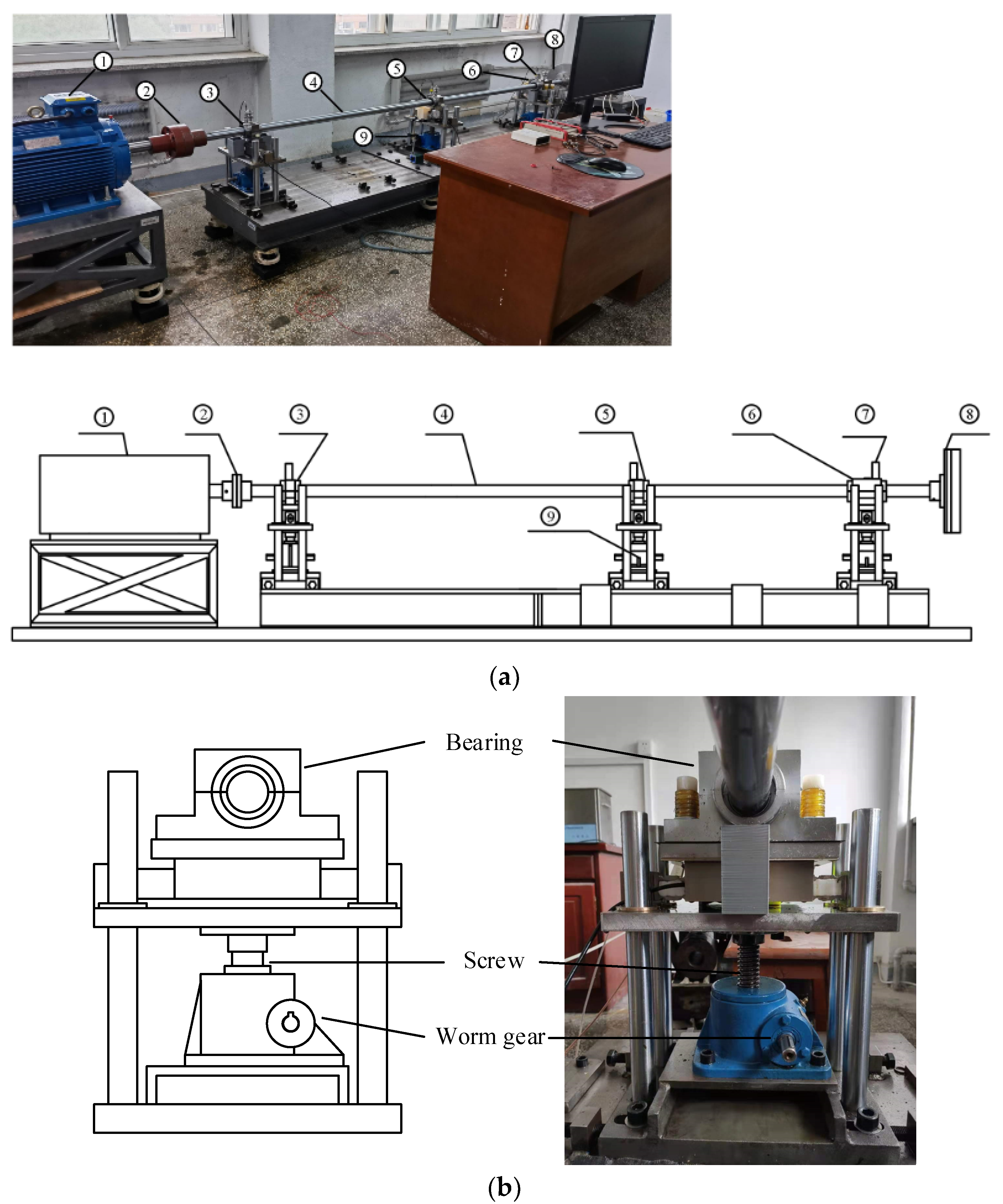
2.1. Experimental Equipment
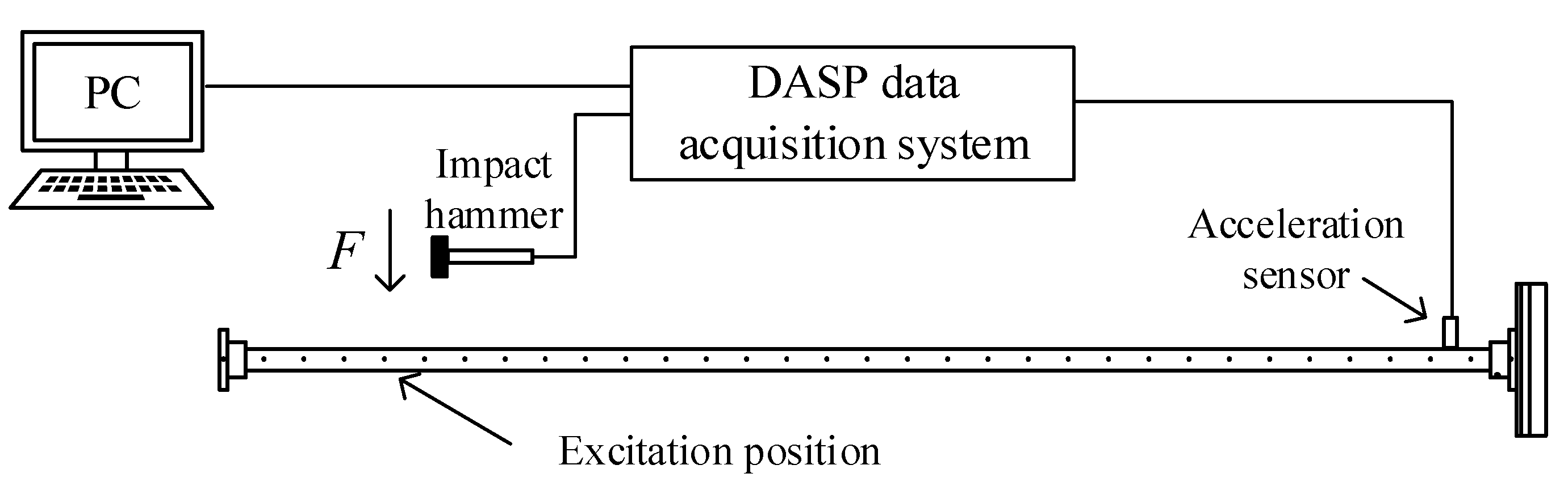
2.2. Experimental Set-Up
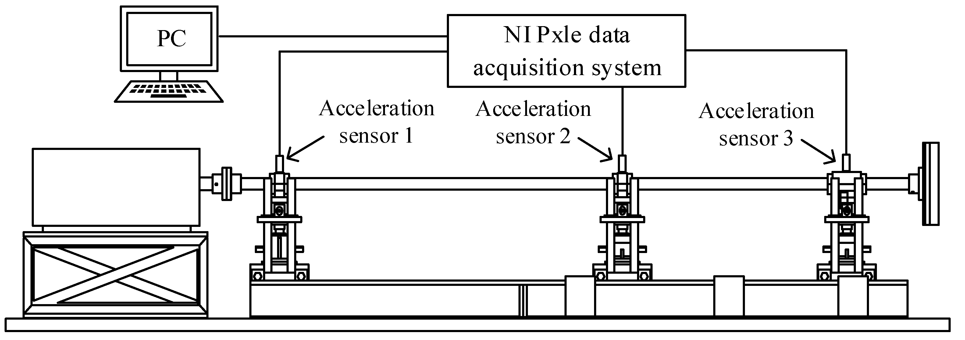
2.3. Collection of Vibration Signal
2.4. Measurement of Natural Frequency
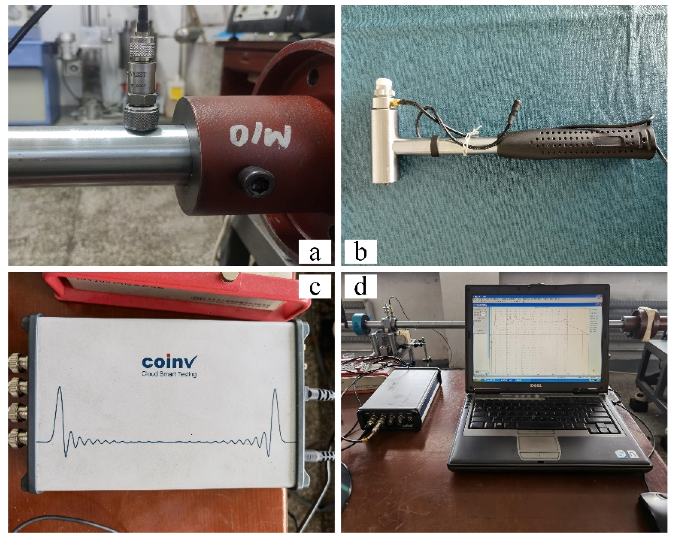
- A uniaxial acceleration sensor (model number: YA-22T) was fixed on the output end of the transmission shaft to measure vibration response.
- The sensitivity of and measurement range of the modal testing hammer (model number: YC-1160401) were 4 mV/N and 0–5 kN, respectively, and the material of the selected hammerhead was nylon.
- Both the impact hammer and the acceleration sensor output were connected to the data acquisition (system model number: INV-3062T). The chassis was connected to the PC, and signals were acquired using DASP V10 (Figure 3).
3. Implementation Approach
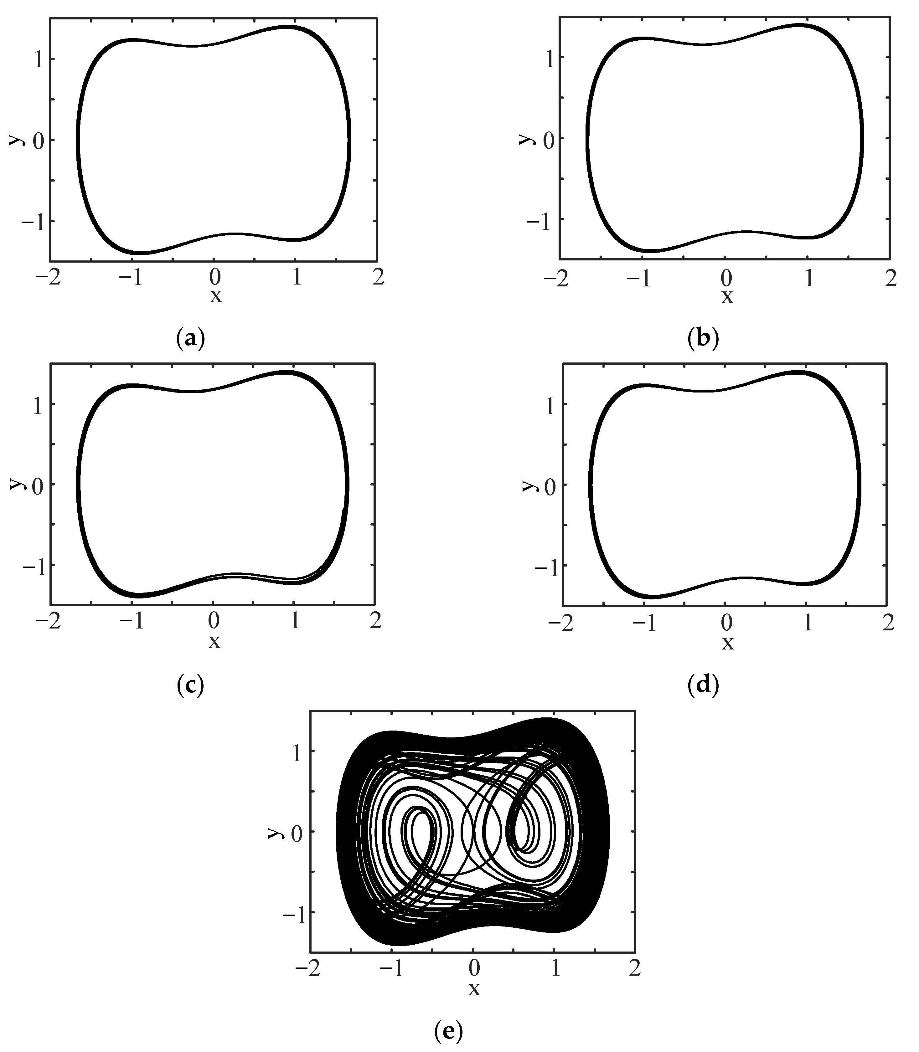
3.1. Detection
3.2. Extraction
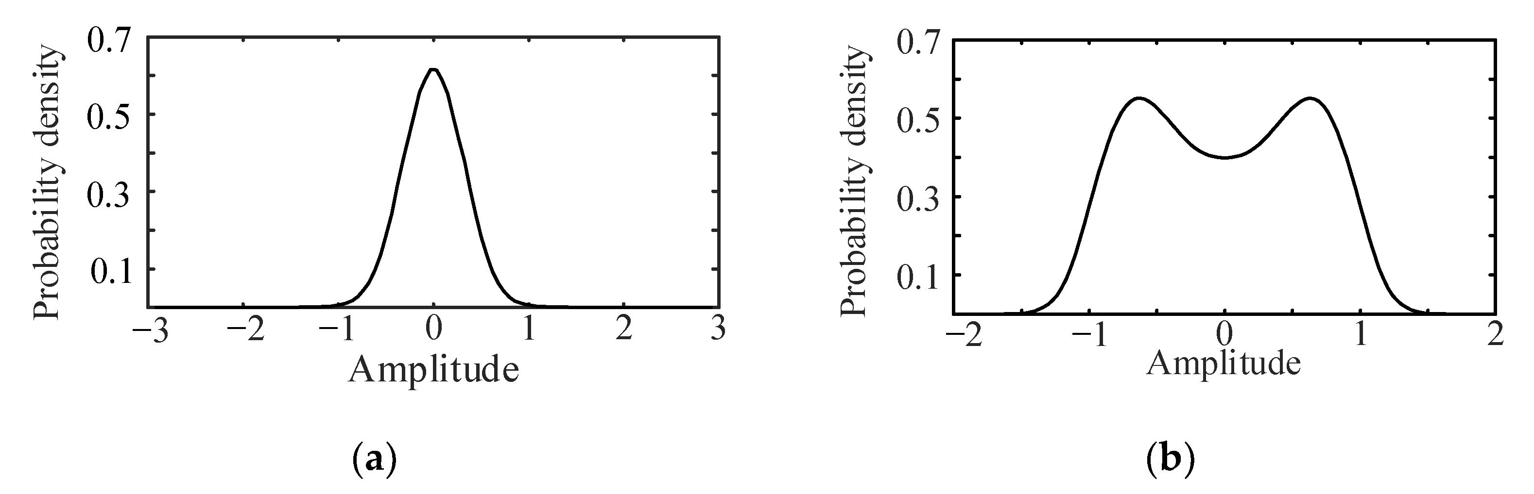
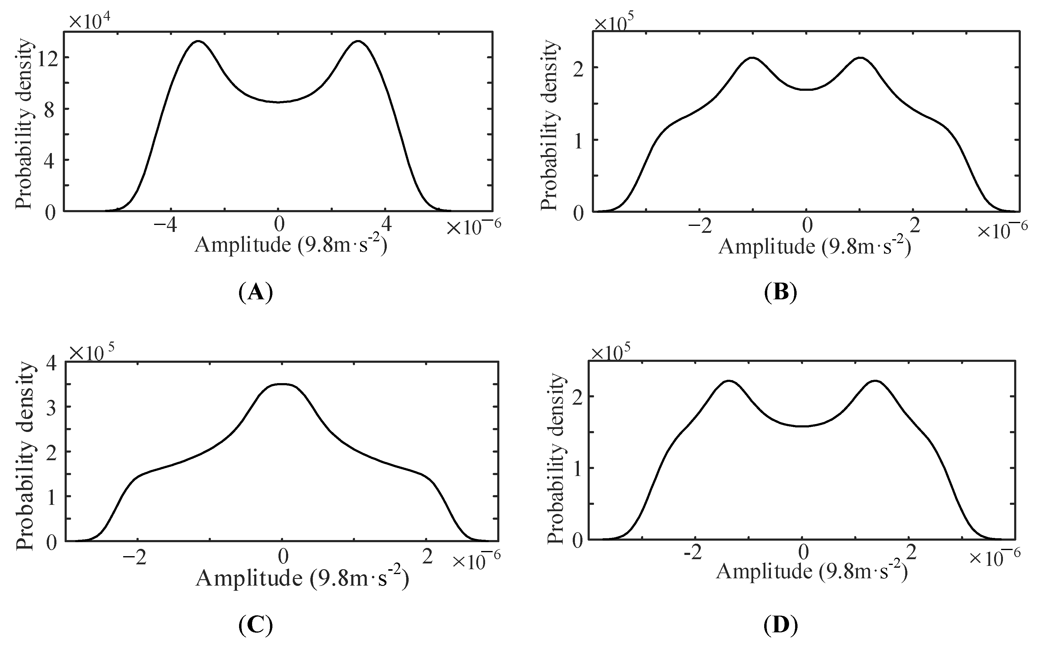
3.3. Identification
4. Results and Discussion
4.1. Acquisition of Natural Frequency Response
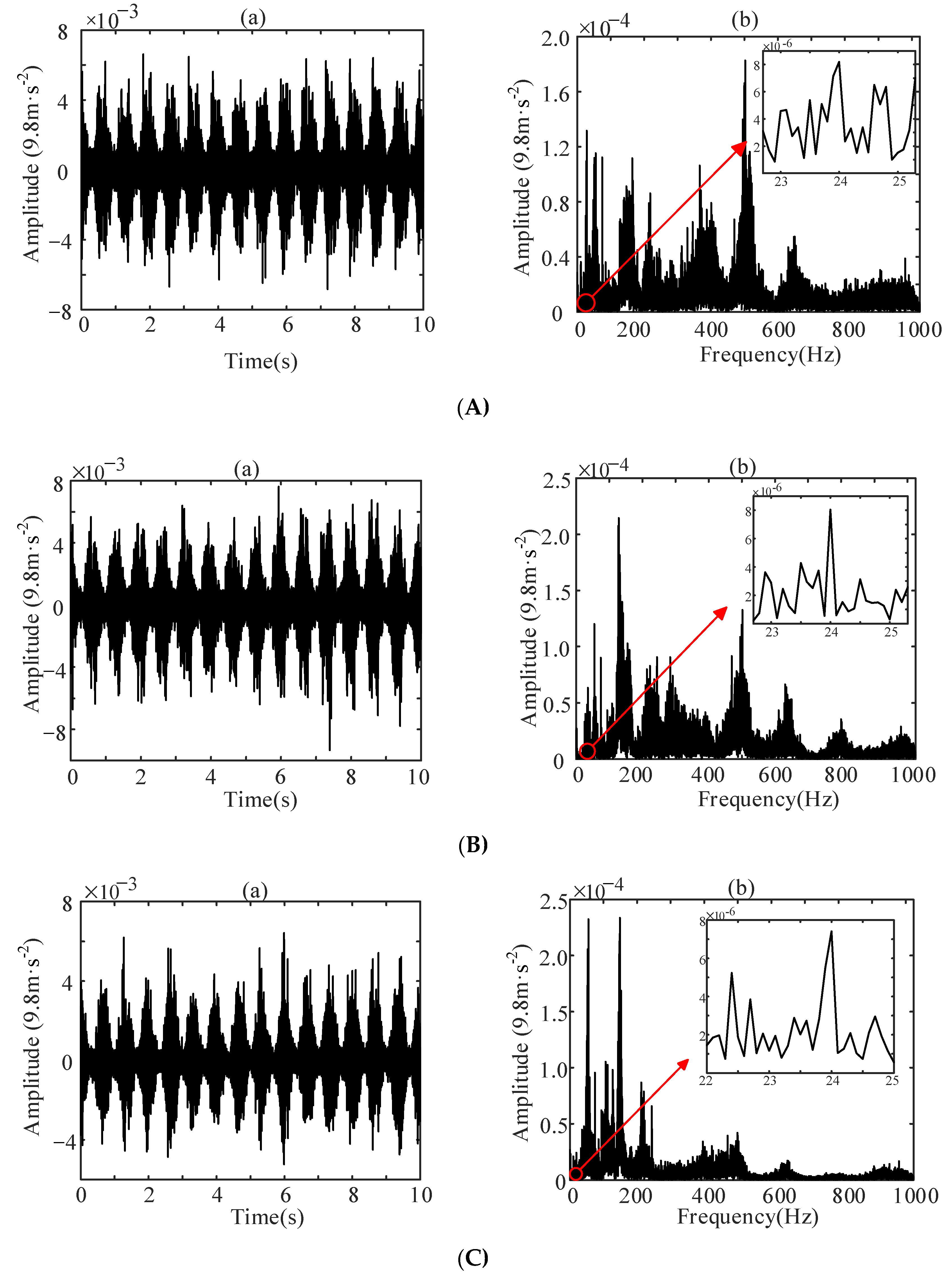
4.1.1. Analysis of Measured Signal
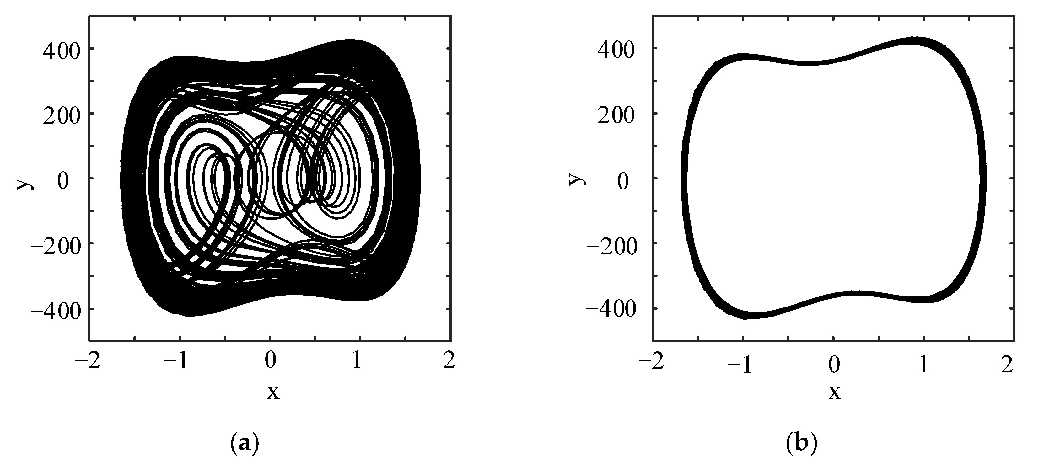
4.1.2. Detection of Measured Signal
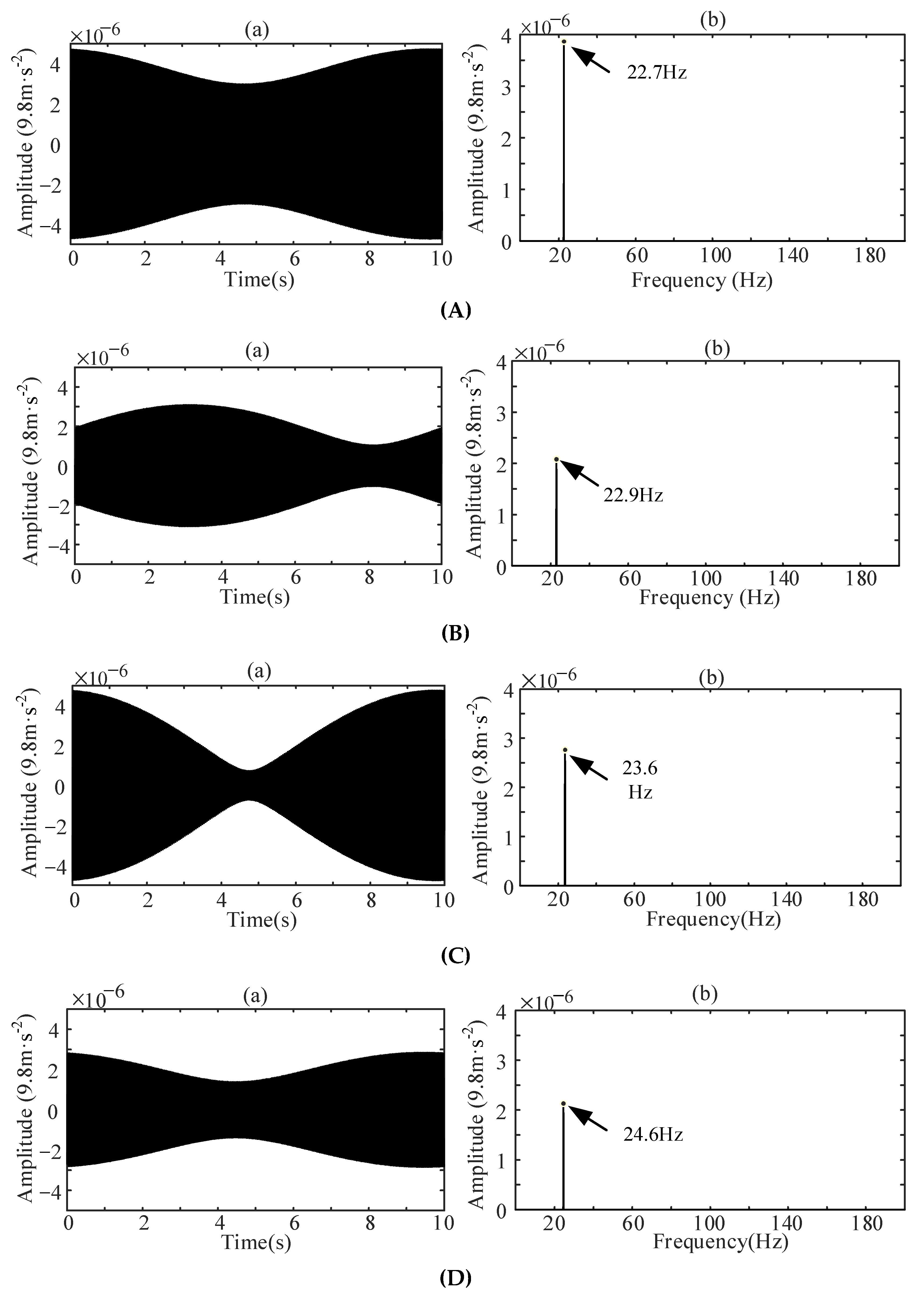
4.1.3. Extraction of Weak Periodic Signal
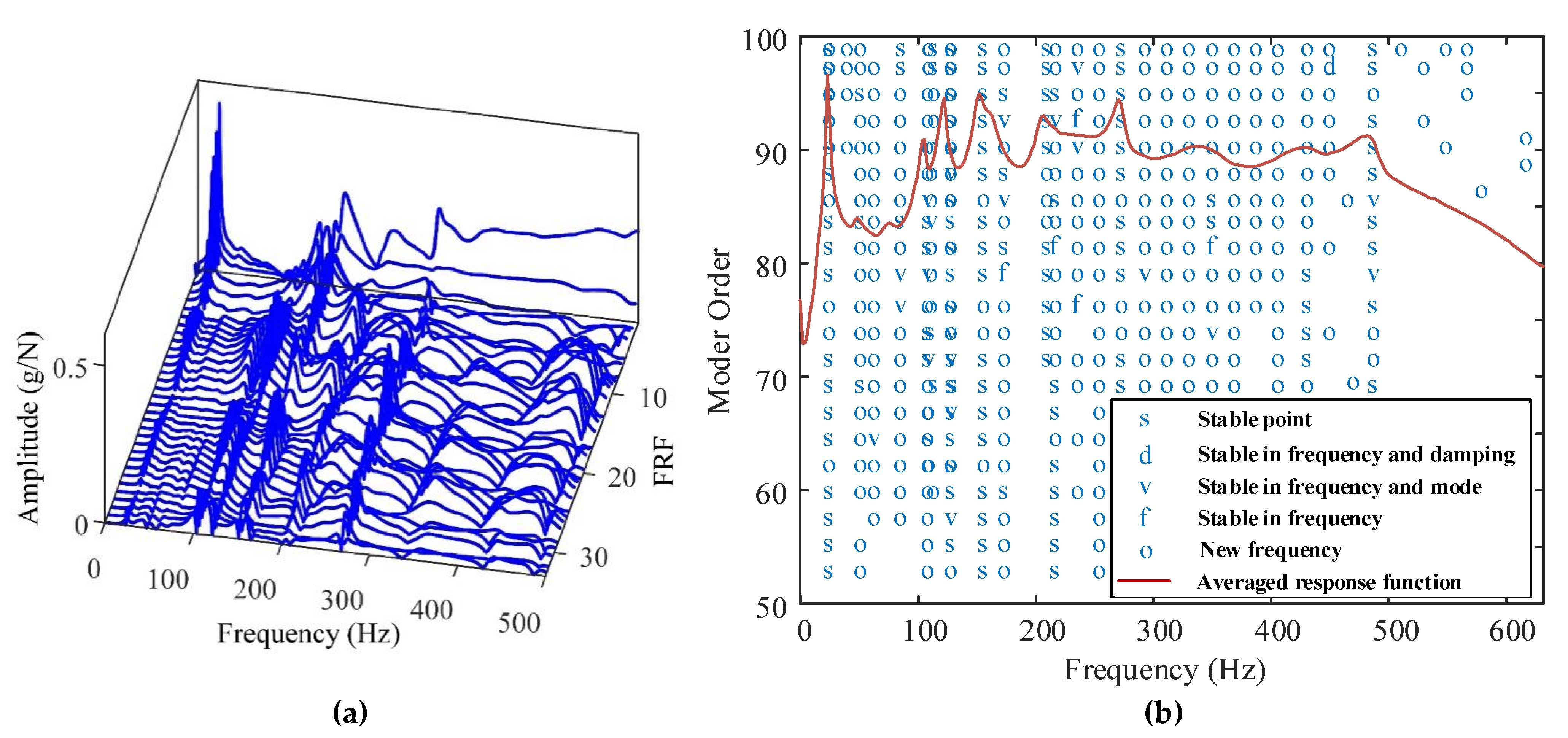
4.1.4. Identification of Extracted Signal
4.2. Variation of Natural Frequency Response under Different Alignment States
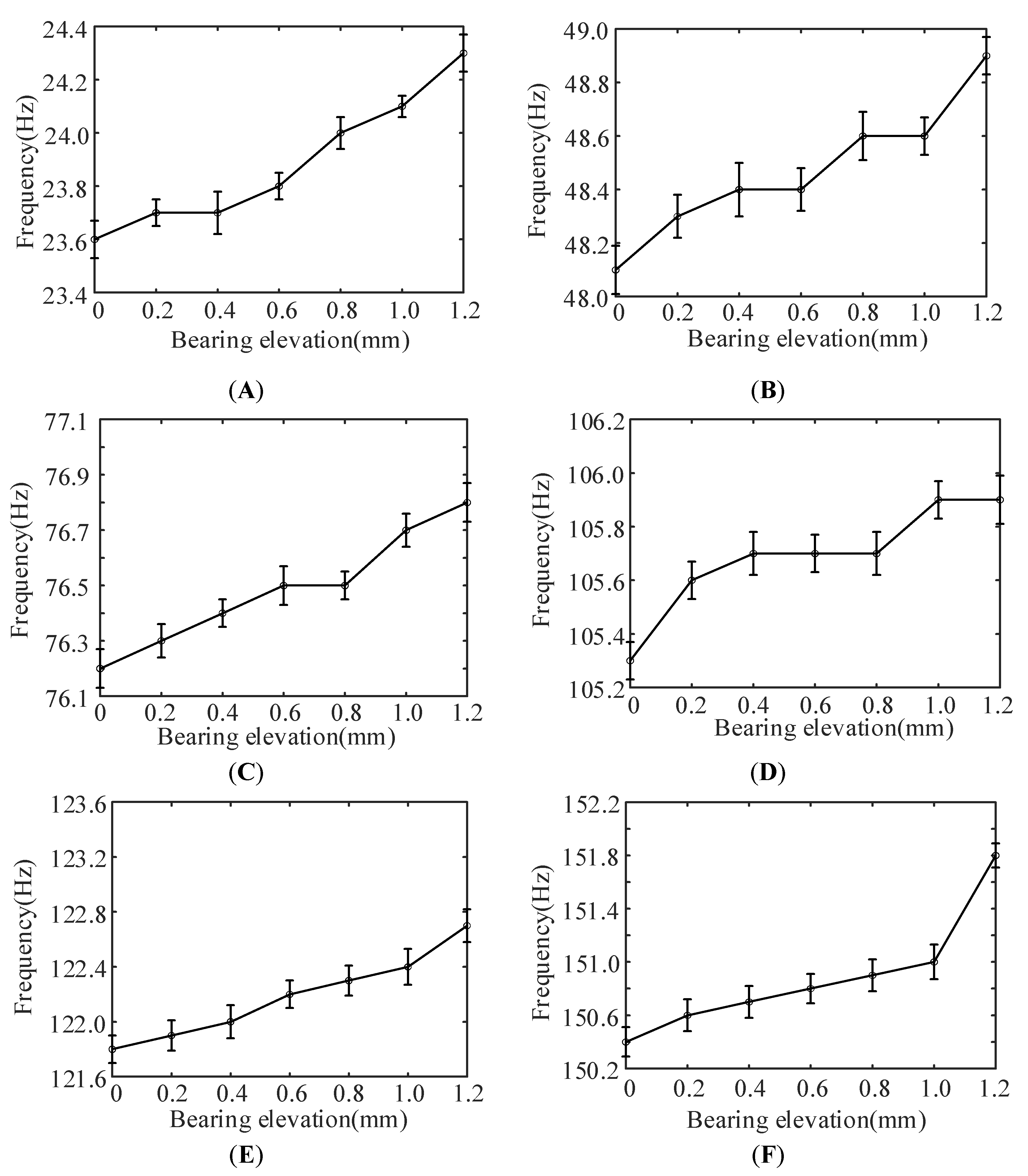
4.2.1. Frequency Changes
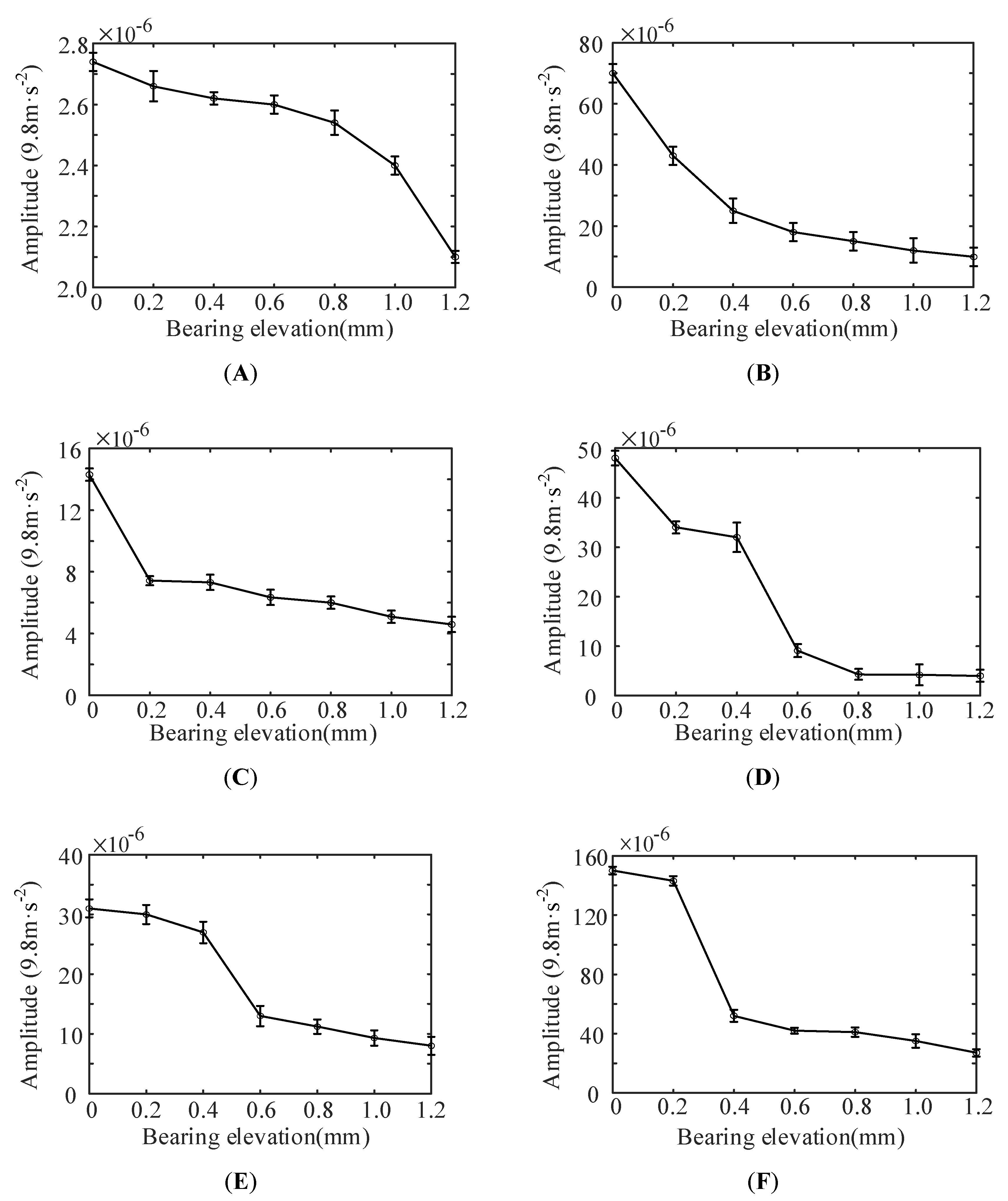
4.2.2. Amplitude Changes
5. Conclusions
- Under the running condition, the natural frequency of the ship propulsion shafting can be excited, and the detection, extraction, and identification of the natural frequency can be achieved using a multi-method approach combining Duffing Oscillator, HWPT, and PDF.
- When the propulsion shafting alignment changes gradually with the increase of elevation of the front stern bearing, the natural frequency increases, and the amplitude decreases. Therefore, the natural frequency can be used to monitor the operating state of the propulsion shafting.
Author Contributions
Funding
Institutional Review Board Statement
Informed Consent Statement
Data Availability Statement
Conflicts of Interest
References
- Zhang, Y.; Lian, J.; Liu, F. An improved filtering method based on EEMD and wavelet-threshold for modal parameter identification of hydraulic structure. Mech. Syst. Signal Process. 2016, 68, 316–329. [Google Scholar] [CrossRef]
- Wang, Z.; Zhang, C.; Tian, Z. Ship Propulsion Shafting Status Monitoring Based on Operational Modal Analysis. Ship Eng. 2017, 39, 183–186+248. [Google Scholar] [CrossRef]
- Xu, Y.F.; Zhu, W.D. Operational modal analysis of a rectangular plate using non-contact excitation and measurement. J. Sound Vib. 2013, 332, 4927–4939. [Google Scholar] [CrossRef]
- Wen, X.; Meng, W.; Sun, X.; Zhou, R. A Composite Method of Marine Shafting’s Fault Diagnosis by Ship Hull Vibrations Based on EEMD. Shock Vib. 2022, 2022, 1236971. [Google Scholar] [CrossRef]
- Murawski, L.; Dereszewski, M. Theoretical and practical backgrounds of monitoring system of ship power transmission systems’ torsional vibration. J. Mar. Sci. Technol. 2020, 25, 272–284. [Google Scholar] [CrossRef] [Green Version]
- Brincker, R.; Zhang, L.; Andersen, P. Modal Identification from ambient Responses Using Frequency Domain Decomposition. 2000. Available online: https://vbn.aau.dk/ws/portalfiles/portal/12765845/Modal_Identification_from_Ambient_Responses_using_Frequency_Domain_Decomposition (accessed on 24 July 2022).
- Van Overschee, P.; De Moor, B. Subspace algorithms for the stochastic identification problem. Automatica 1993, 29, 649–660. [Google Scholar] [CrossRef]
- Juang, J.-N.; Pappa, R.S. An eigensystem realization algorithm for modal parameter identification and model reduction. J. Guid. Control Dyn. 1985, 8, 620–627. [Google Scholar] [CrossRef] [Green Version]
- Mignolet, M.P.; Soize, C. Nonparametric stochastic modeling of linear systems with prescribed variance of several natural frequencies. Probabilistic Eng. Mech. 2008, 23, 267–278. [Google Scholar] [CrossRef] [Green Version]
- Xue, S.; Wu, S.; Tang, Q.; Liu, S.; Liu, B. Research on torsional vibration monitoring system of ship power shafting. IOP Conf. Ser. Mater. Sci. Eng. 2021, 1207, 012007. [Google Scholar] [CrossRef]
- Akilli, M. Detecting weak periodic signals in EEG time series. Chin. J. Phys. 2016, 54, 77–85. [Google Scholar] [CrossRef]
- Akilli, M.; Yilmaz, N.; Akdeniz, K.G. Automated system for weak periodic signal detection based on Duffing oscillator. IET Signal Process. 2020, 14, 710–716. [Google Scholar] [CrossRef]
- Wang, K.; Yan, X.; Yang, Q.; Hao, X.; Wang, J. Weak signal detection based on strongly coupled Duffing-Van der Pol oscillator and long short-term memory. J. Phys. Soc. Jpn. 2020, 89, 014003. [Google Scholar] [CrossRef]
- Hu, N.Q.; Wen, X.S. The application of Duffing oscillator in characteristic signal detection of early fault. J. Sound Vib. 2003, 268, 917–931. [Google Scholar] [CrossRef]
- Heo, Y.; Kim, K.-j. Definitions of non-stationary vibration power for time–frequency analysis and computational algorithms based upon harmonic wavelet transform. J. Sound Vib. 2015, 336, 275–292. [Google Scholar] [CrossRef]
- Yan, R.; Gao, R.X. An efficient approach to machine health diagnosis based on harmonic wavelet packet transform. Robot. Comput.-Integr. Manuf. 2005, 21, 291–301. [Google Scholar] [CrossRef]
- Brincker, R.; Andersen, P.; Møller, N. An indicator for Separation of Structural and Harmonic Modes in Output-Only Modal Testing, Universidad Politécnica de Madrid. 2000, pp. 265–272. Available online: https://vbn.aau.dk/en/publications/an-indicator-for-separation-of-structural-and-harmonic-modes-in-o (accessed on 24 July 2022).
- Nadkarni, I.; Bhardwaj, R.; Ninan, S.; Chippa, S.P. Experimental modal parameter identification and validation of cantilever beam. Mater. Today-Proc. 2021, 38, 319–324. [Google Scholar] [CrossRef]
- Wang, G.; Chen, D.; Lin, J.; Chen, X. The application of chaotic oscillators to weak signal detection. IEEE Trans. Ind. Electron. 1999, 46, 440–444. [Google Scholar] [CrossRef]
- Akilli, M.; Yilmaz, N. Study of weak periodic signals in the EEG signals and their relationship with postsynaptic potentials. IEEE Trans. Neural Syst. Rehabil. Eng. 2018, 26, 1918–1925. [Google Scholar] [CrossRef] [PubMed]
- Dong, X.; Lian, J.; Yang, M.; Wang, H. Operational modal identification of offshore wind turbine structure based on modified stochastic subspace identification method considering harmonic interference. J. Renew. Sustain. Energy 2014, 6, 033128. [Google Scholar] [CrossRef]


| Order-Number | 1 | 2 | 3 | 4 | 5 | 6 |
|---|---|---|---|---|---|---|
| Natural frequency/Hz | 23.8 | 47.9 | 75.8 | 105.7 | 122.5 | 151.5 |
| Order-Number | 1 | 2 | 3 | 4 | 5 | 6 |
|---|---|---|---|---|---|---|
| Natural frequency (Hz) | 23.8 | 47.9 | 75.8 | 105.7 | 122.5 | 151.5 |
| Detection band (Hz) | 22.3~25.3 | 46.4~49.4 | 74.3~76.3 | 104.2~107.2 | 121.0~124.0 | 150.0~153.0 |
| Reference signal amplitude | 0.8265 | 0.8264 | 0.8263 | 0.8281 | 0.8305 | 0.8387 |
| Frequency Band (Hz) | 22.3~25.3 | 46.4~49.4 | 74.3~77.3 | 104.2~107.2 | 121.0~124.0 | 150.0~153.0 |
|---|---|---|---|---|---|---|
| Frequency of the periodic signal (Hz) | 22.7 | 47.0 | 75.4 | 105.1 | 121.8 | 150.4 |
| 22.9 | 47.8 | 75.9 | 105.3 | 122.3 | 150.7 | |
| 23.6 | 48.1 | 76.2 | 105.5 | 122.5 | 151.3 | |
| 24.6 | 49.0 |
| Order-Number | 1 | 2 | 3 | 4 | 5 | 6 | |
|---|---|---|---|---|---|---|---|
| Measuring Position | |||||||
| Aft stern bearing/Hz | 23.6 | 48.1 | 76.2 | 105.3 | 121.8 | 150.4 | |
| Front stern bearing/Hz | 23.6 | 47.8 | 75.8 | 105.5 | 122.1 | 150.7 | |
| Intermediate bearing/Hz | 23.1 | 47.5 | 75.0 | 105.3 | 122.2 | 150.4 | |
| Standard deviation | 0.289 | 0.300 | 0.611 | 0.116 | 0.208 | 0.173 | |
Publisher’s Note: MDPI stays neutral with regard to jurisdictional claims in published maps and institutional affiliations. |
© 2022 by the authors. Licensee MDPI, Basel, Switzerland. This article is an open access article distributed under the terms and conditions of the Creative Commons Attribution (CC BY) license (https://creativecommons.org/licenses/by/4.0/).
Share and Cite
Xing, P.; Lu, L.; Li, G.; Wang, X.; Gao, H.; Song, Y.; Zhang, H. A Multi-Method Approach to Identify the Natural Frequency of Ship Propulsion Shafting under the Running Condition. J. Mar. Sci. Eng. 2022, 10, 1432. https://doi.org/10.3390/jmse10101432
Xing P, Lu L, Li G, Wang X, Gao H, Song Y, Zhang H. A Multi-Method Approach to Identify the Natural Frequency of Ship Propulsion Shafting under the Running Condition. Journal of Marine Science and Engineering. 2022; 10(10):1432. https://doi.org/10.3390/jmse10101432
Chicago/Turabian StyleXing, Pengfei, Lixun Lu, Guobin Li, Xin Wang, Honglin Gao, Yuchao Song, and Hongpeng Zhang. 2022. "A Multi-Method Approach to Identify the Natural Frequency of Ship Propulsion Shafting under the Running Condition" Journal of Marine Science and Engineering 10, no. 10: 1432. https://doi.org/10.3390/jmse10101432