
Development of Discrete-Time Waterjet Control Systems Used in Surface Vehicle Thrust Vectoring


Abstract
:1. Introduction
2. Materials and Methods
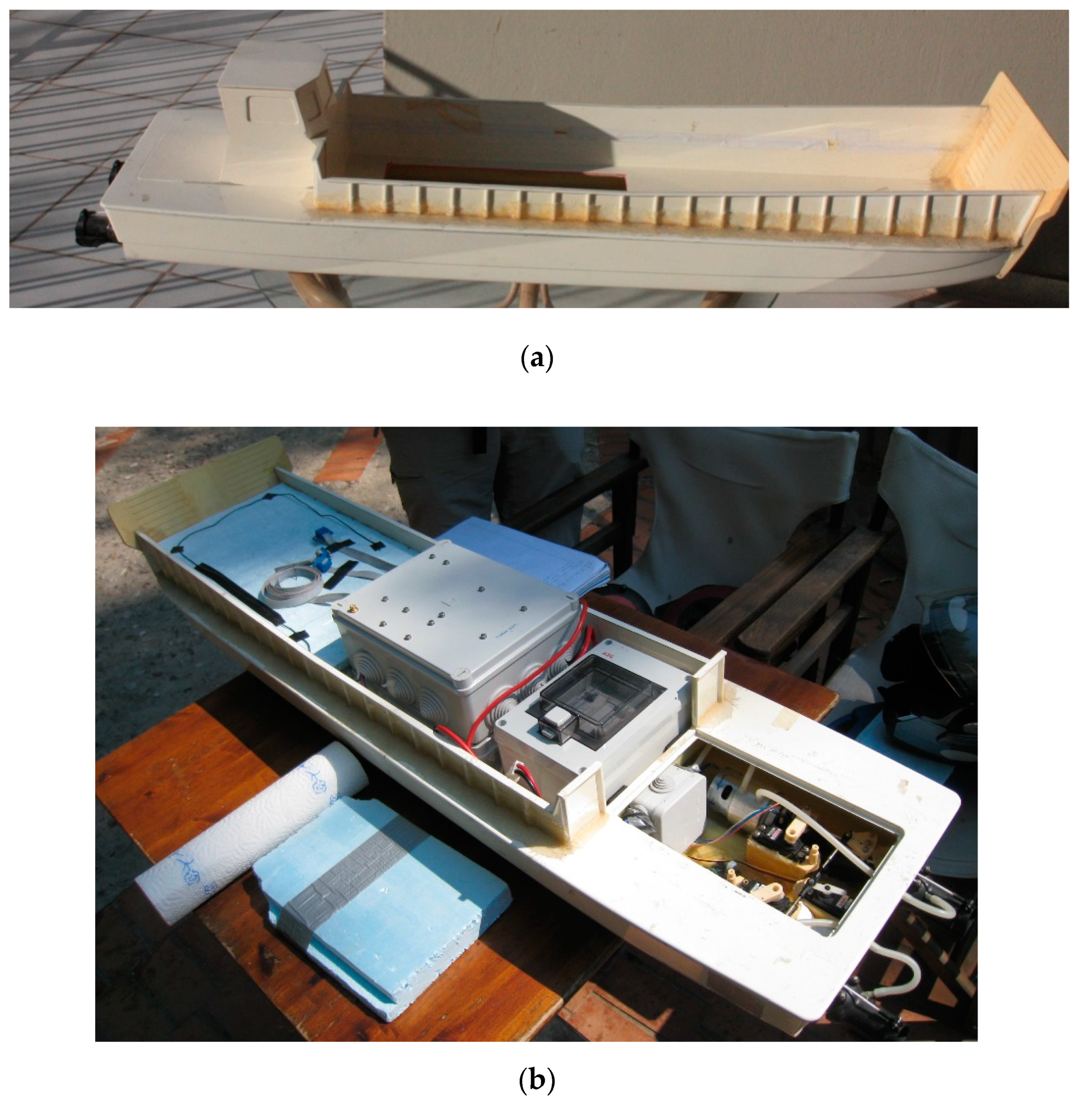
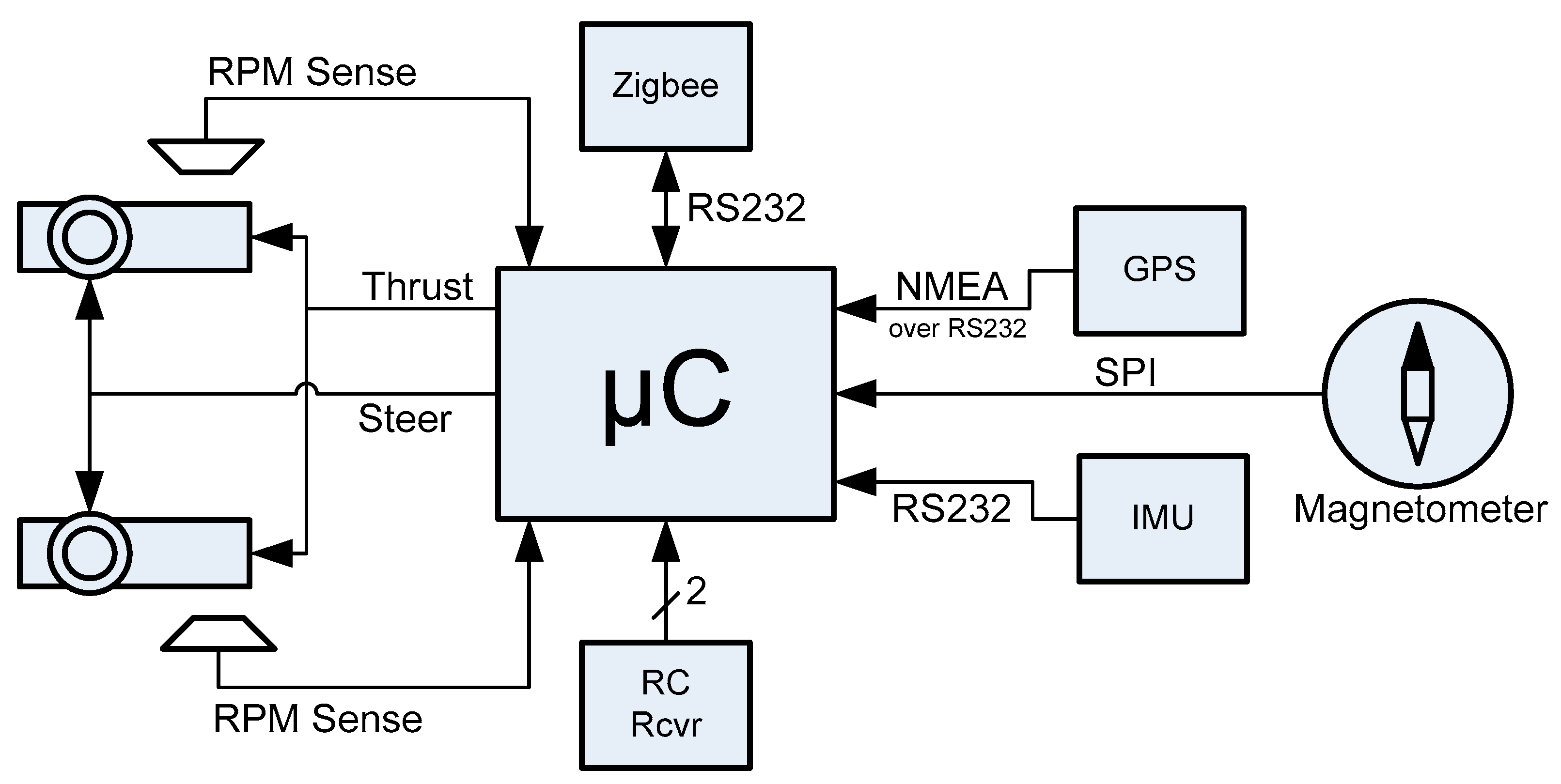
3. Development Platform
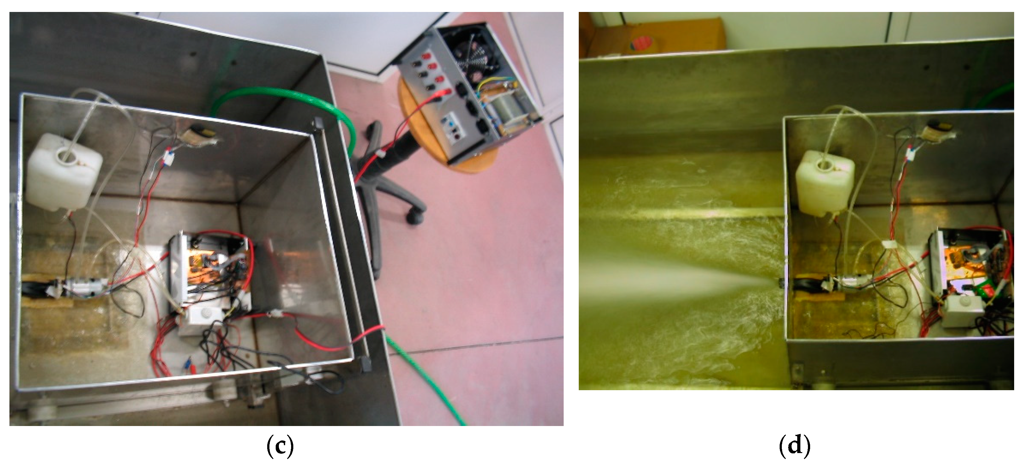
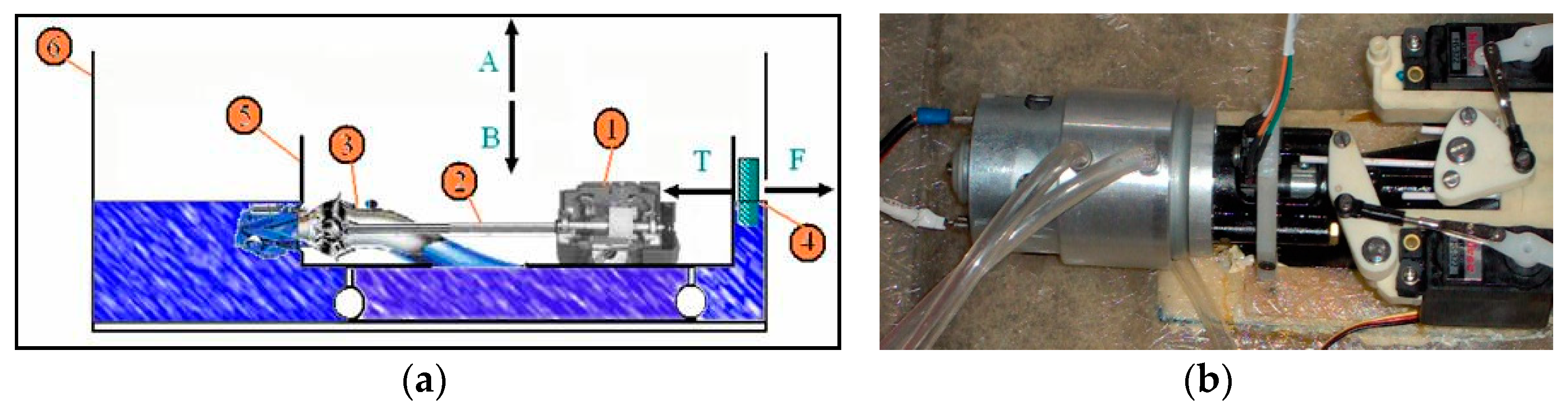
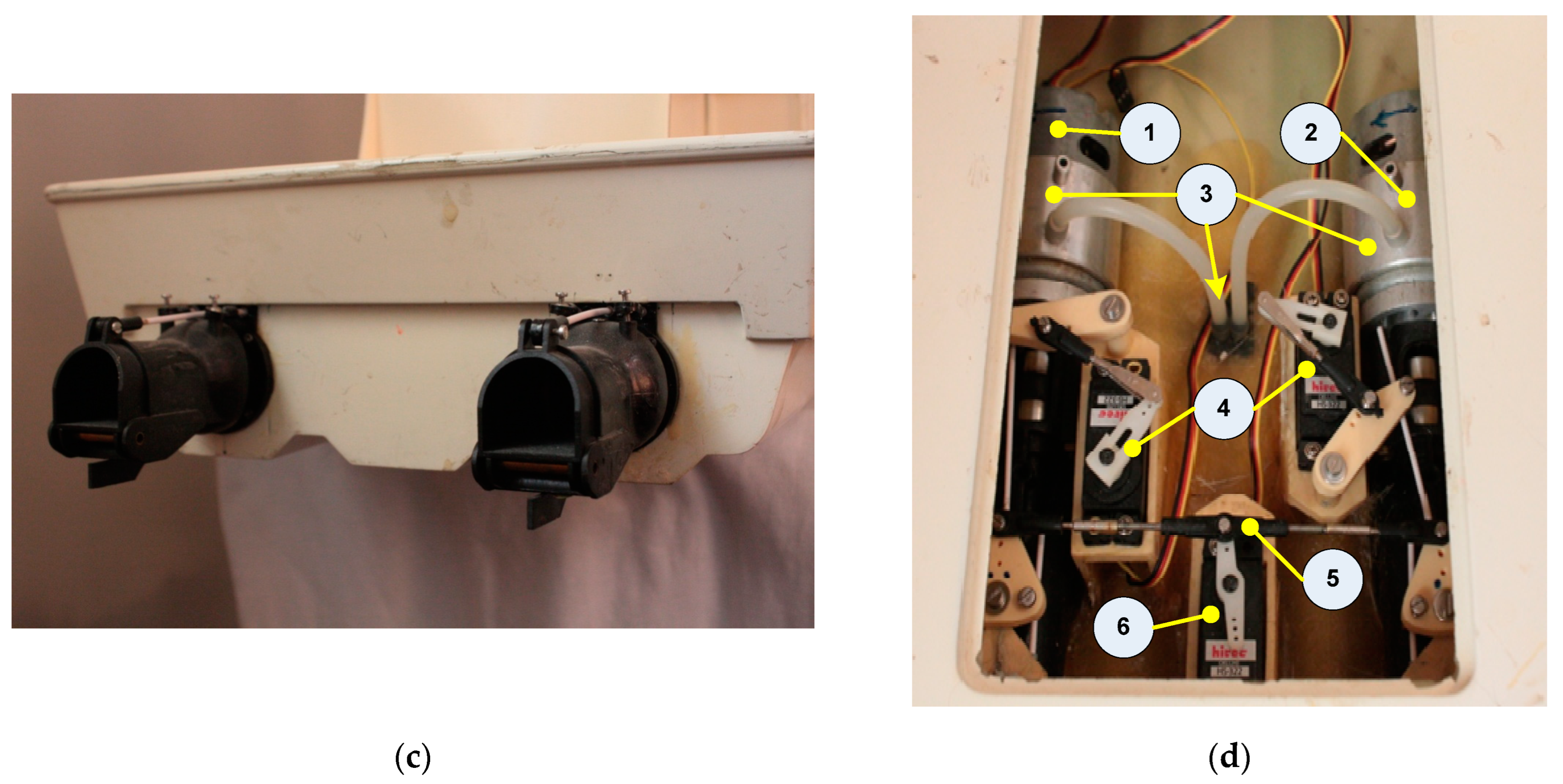
- Electric motors. These motors provide the thrust for waterjet propellers.
- External cooling ring that encapsulates the motors. As the vessel surge velocity increases, an amount of water is forced into the silicone tubes shown by number (3). The water circulates at the outer ring cooling the motors and is rejected from another silicone tube not yet attached at the time this photo was taken.
- Silicone tubes and input of water for motor cooling.
- Servos controlling the backward fin that changes the direction of propulsion (forward—backward movement).
- Shaft that joins the two waterjets for simultaneous turning (left right).
- The servo motor that is used for turning the waterjets.
4. Introductory Concepts
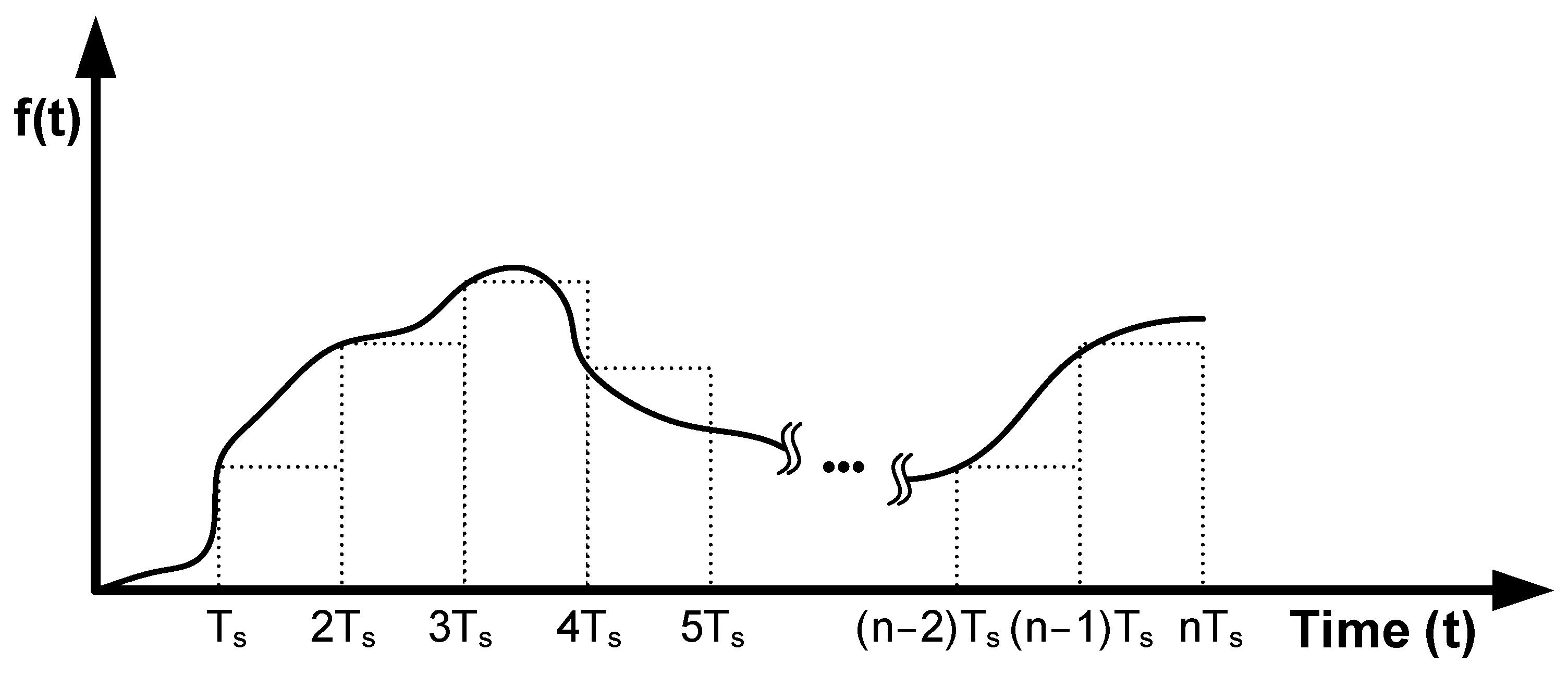
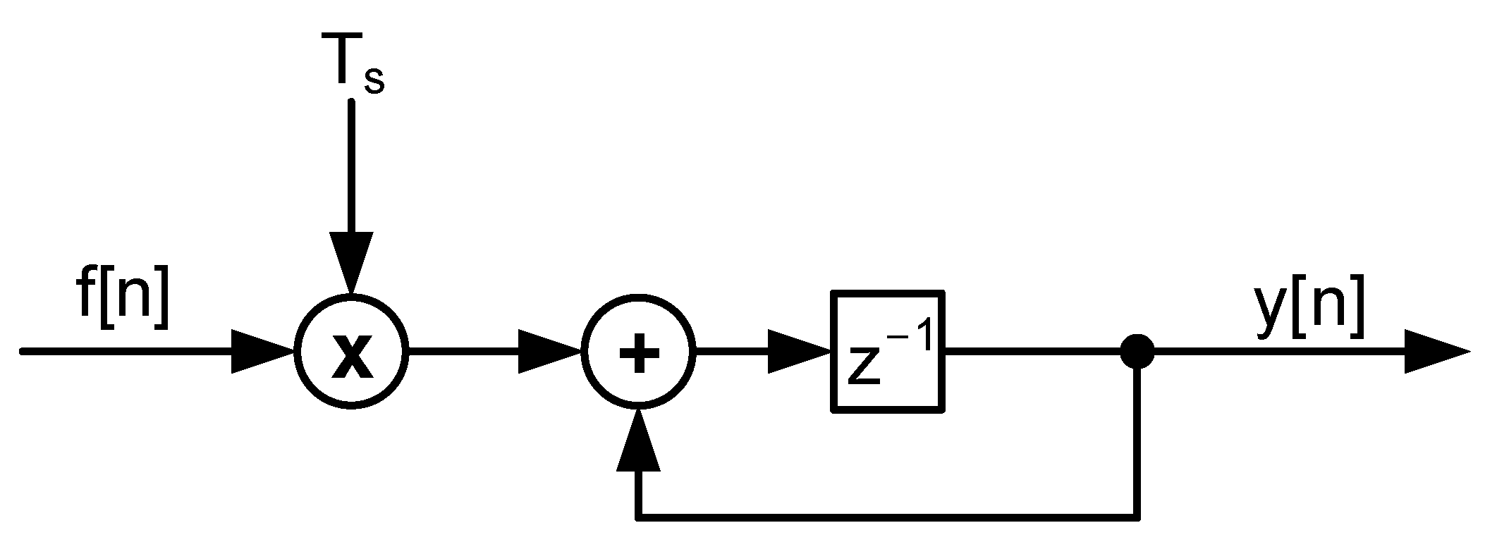
5. Summation Approximation to Integral
6. Digitizing the Analog PID Functionality
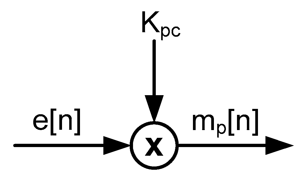
6.1. P-Term
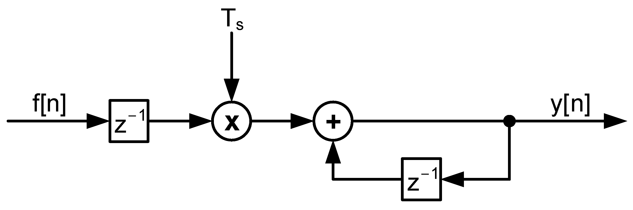
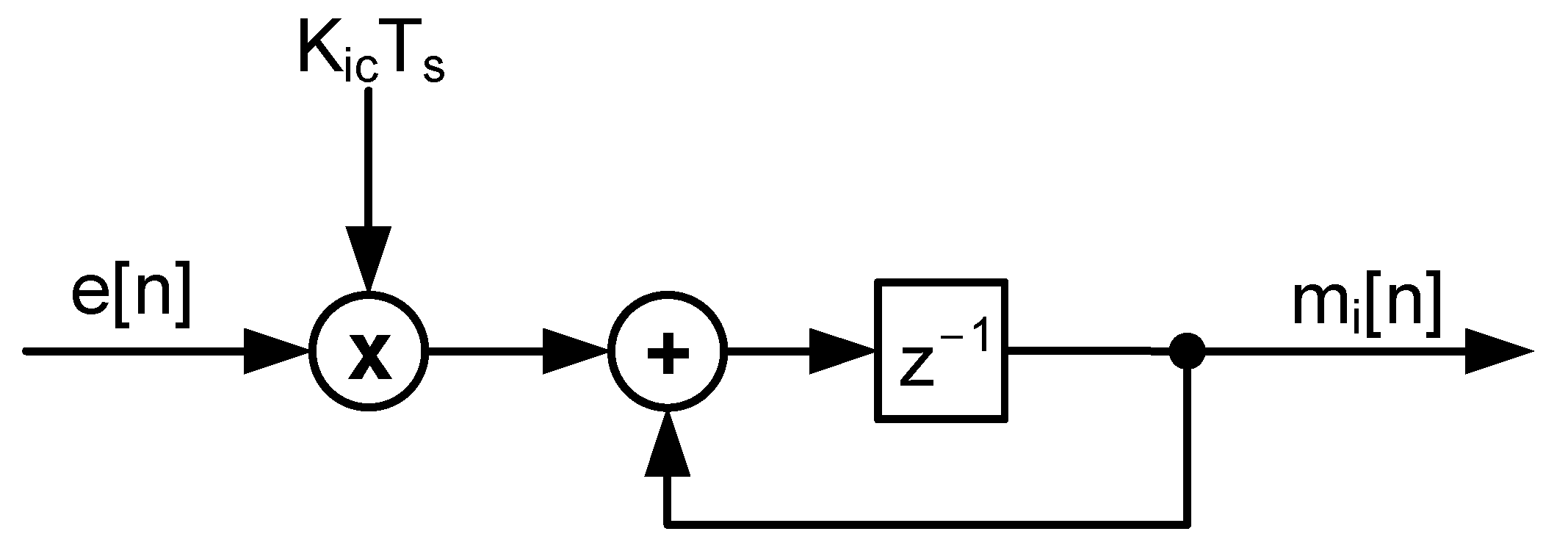
6.2. I-Term
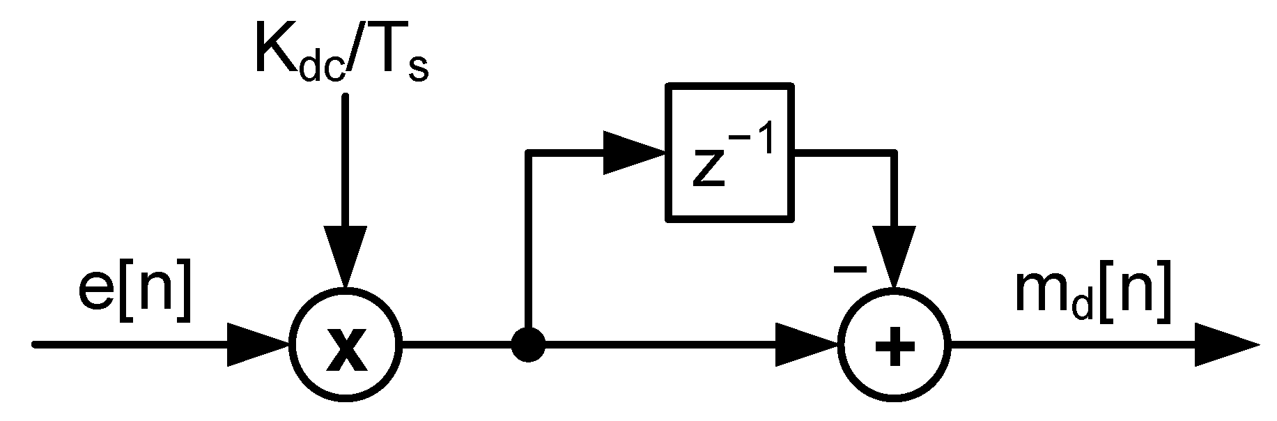
6.3. D-Term
6.4. Combining All Terms
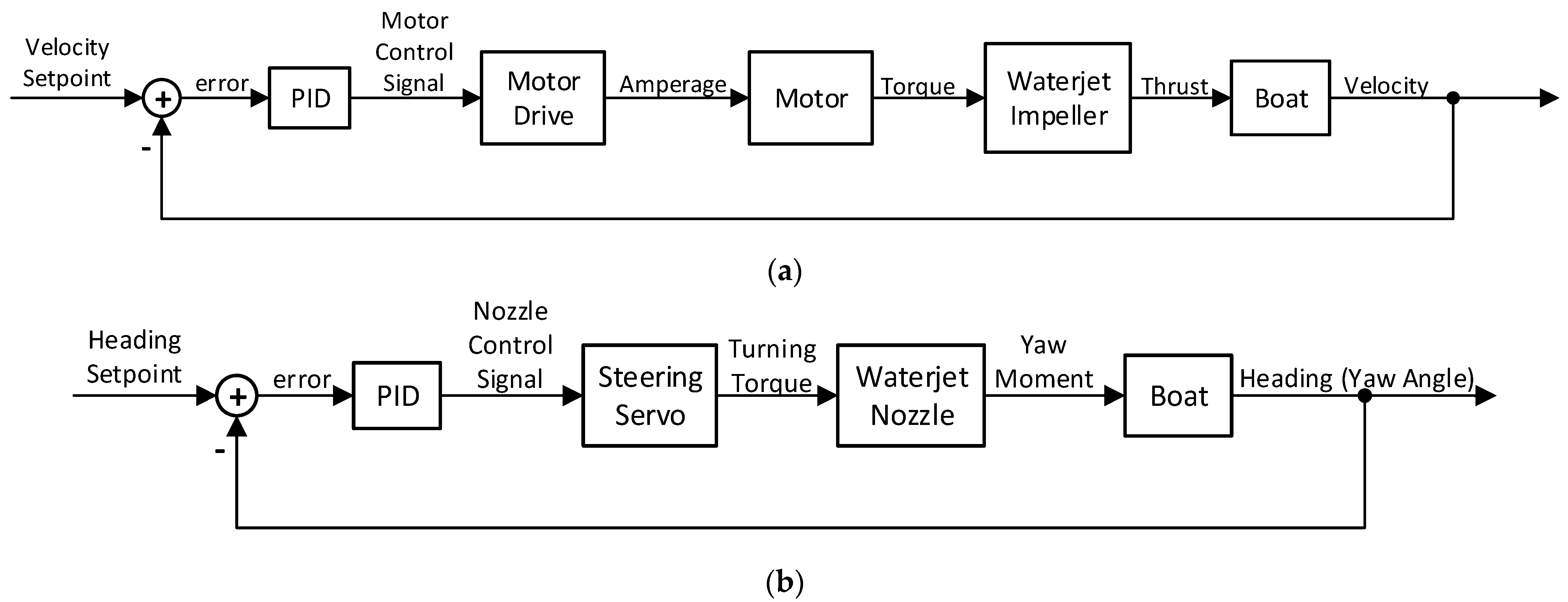
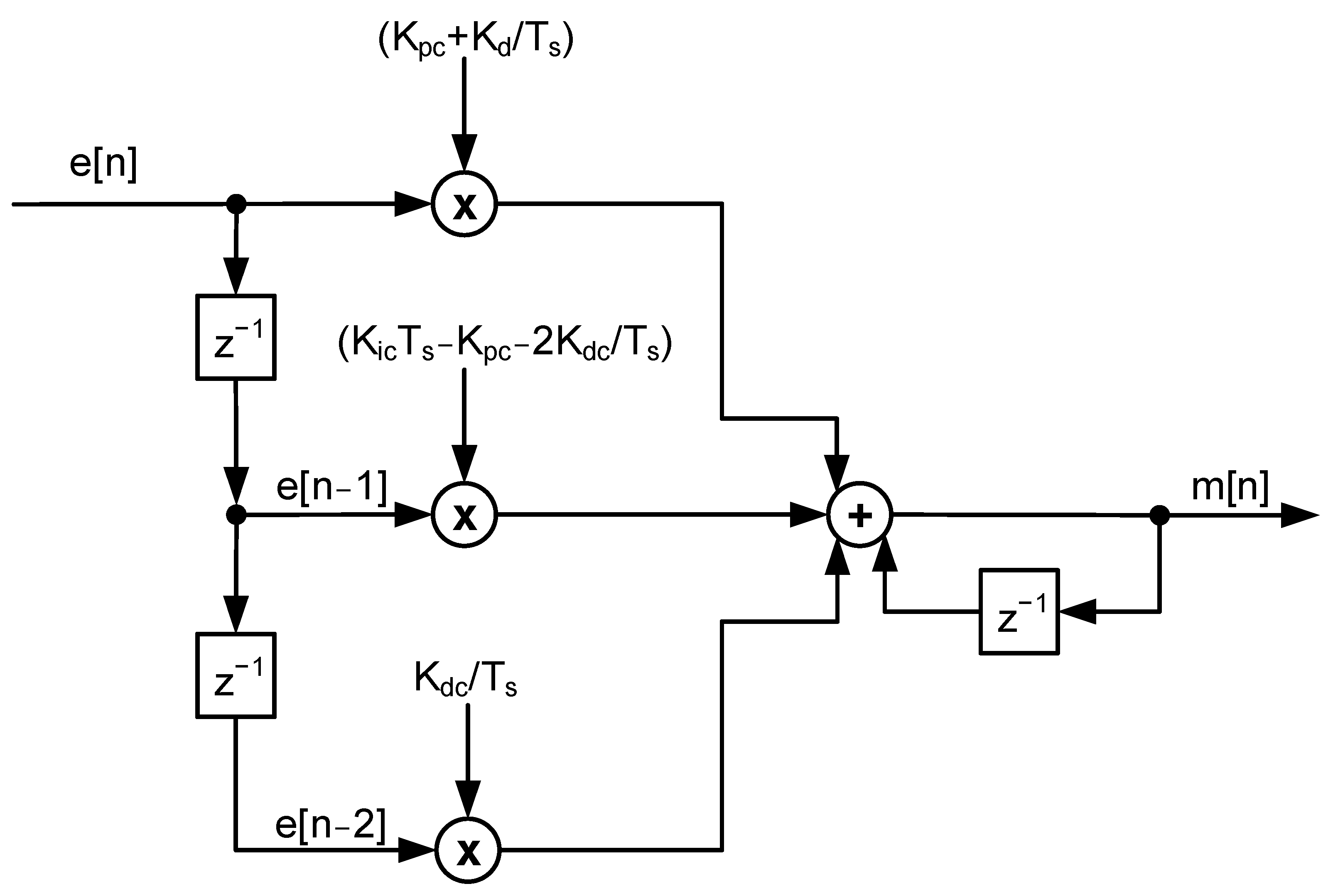
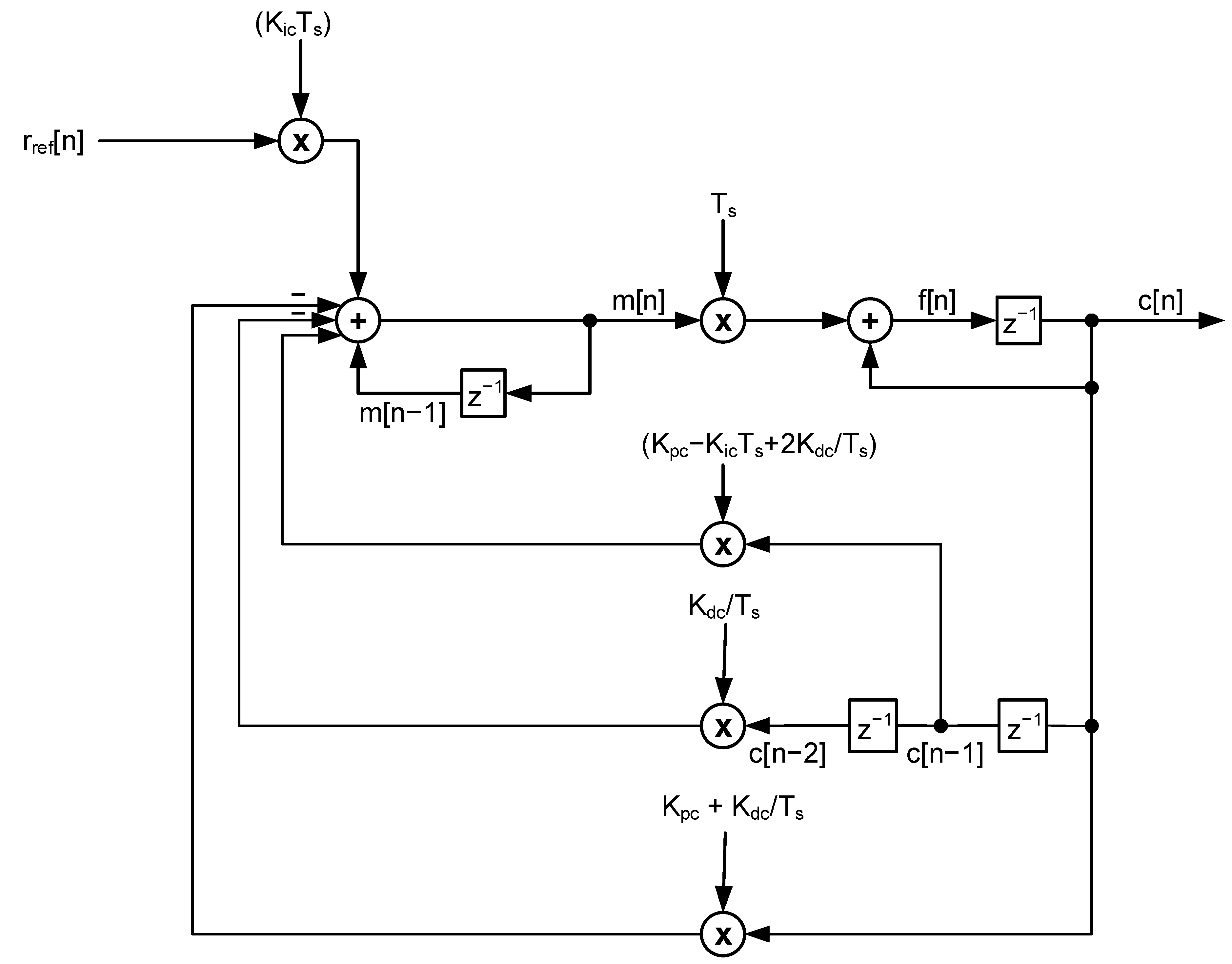
7. Block Diagrams for Digital PID
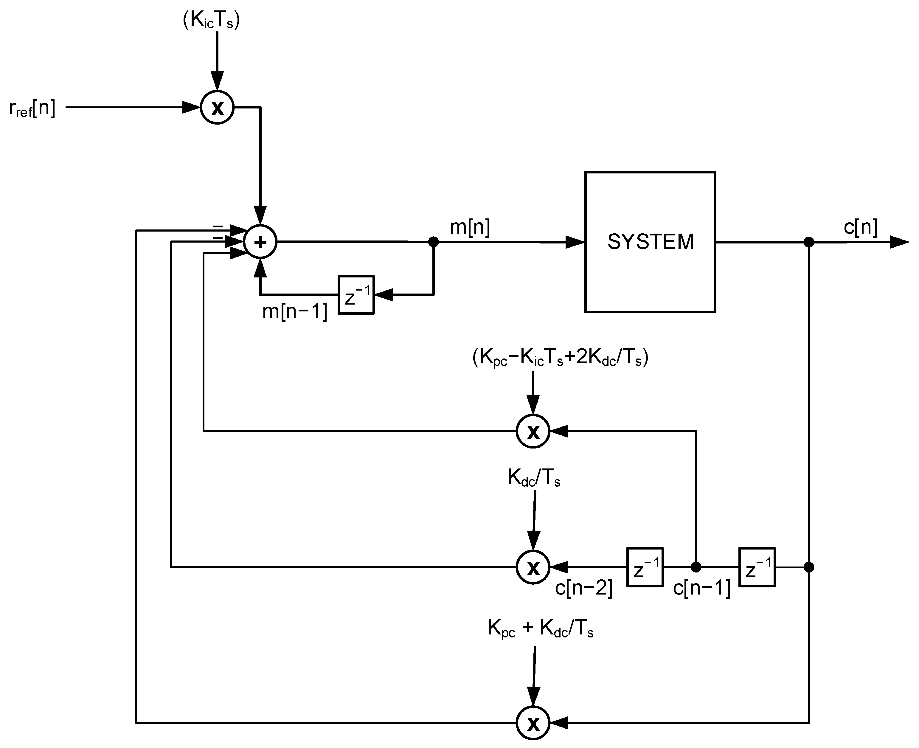
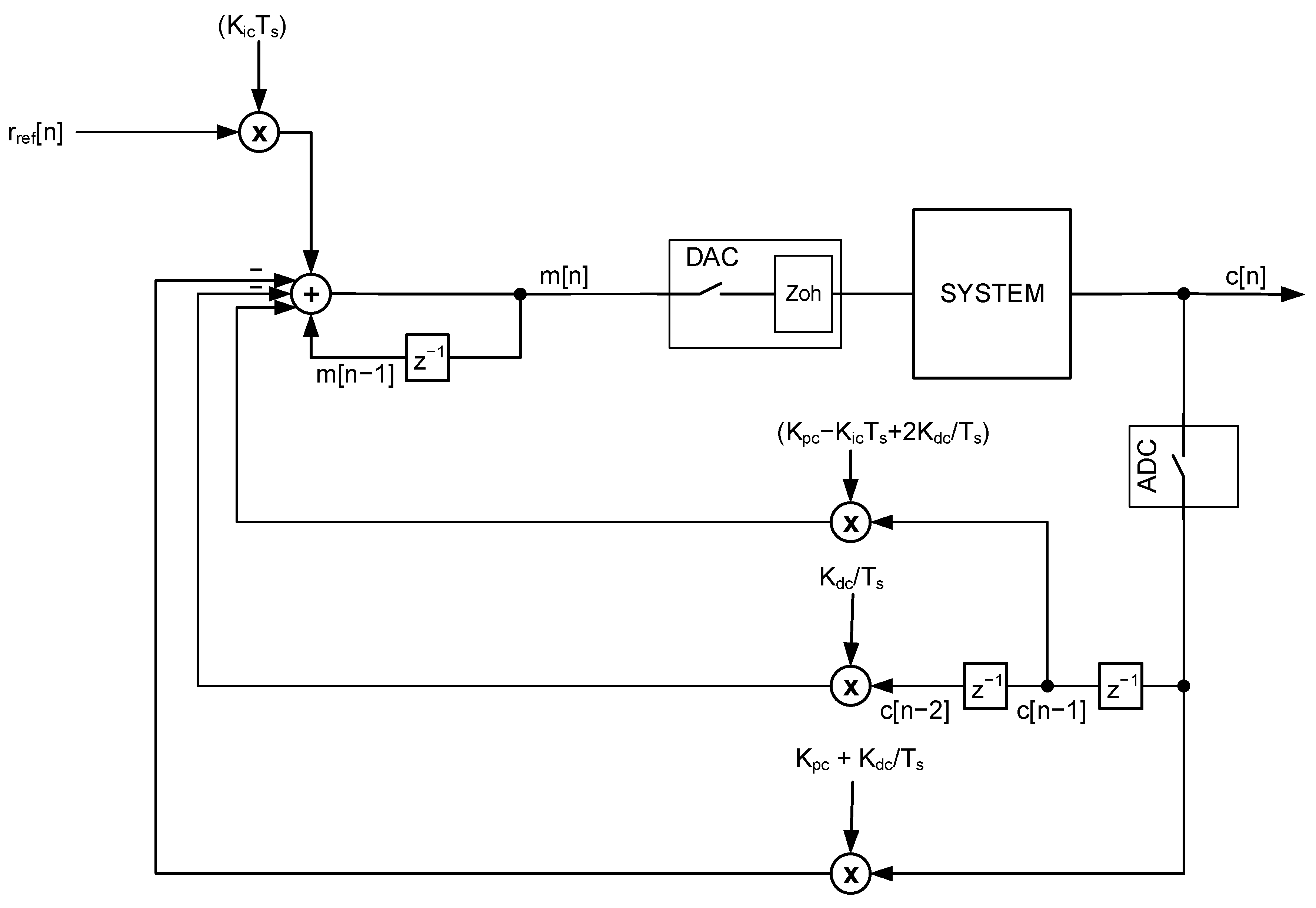
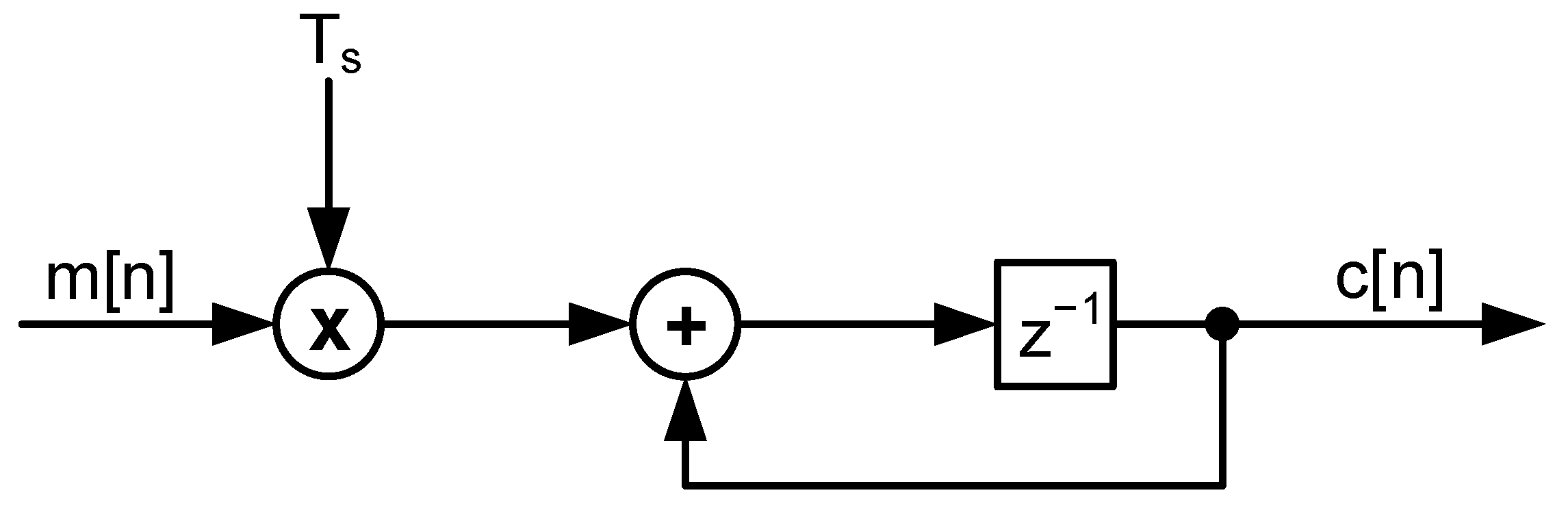
8. Alternative PID Implementation (Velocity Form)
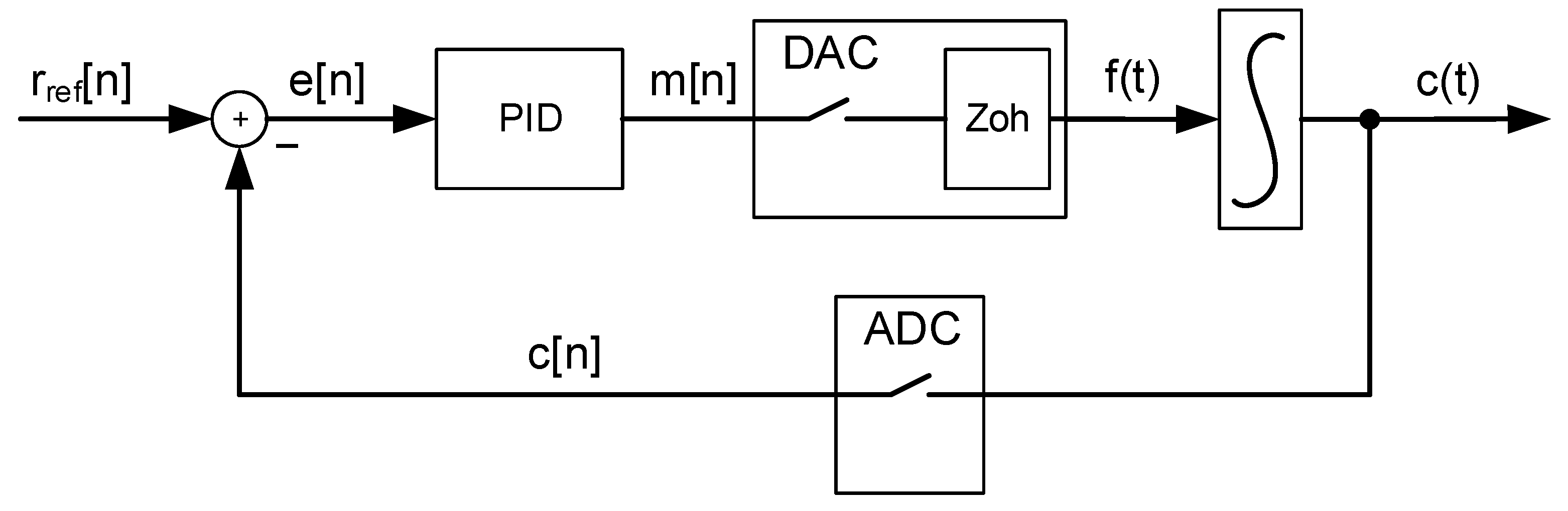
9. Test Bed for PID Control
10. Mathematical Analysis in Discrete Time
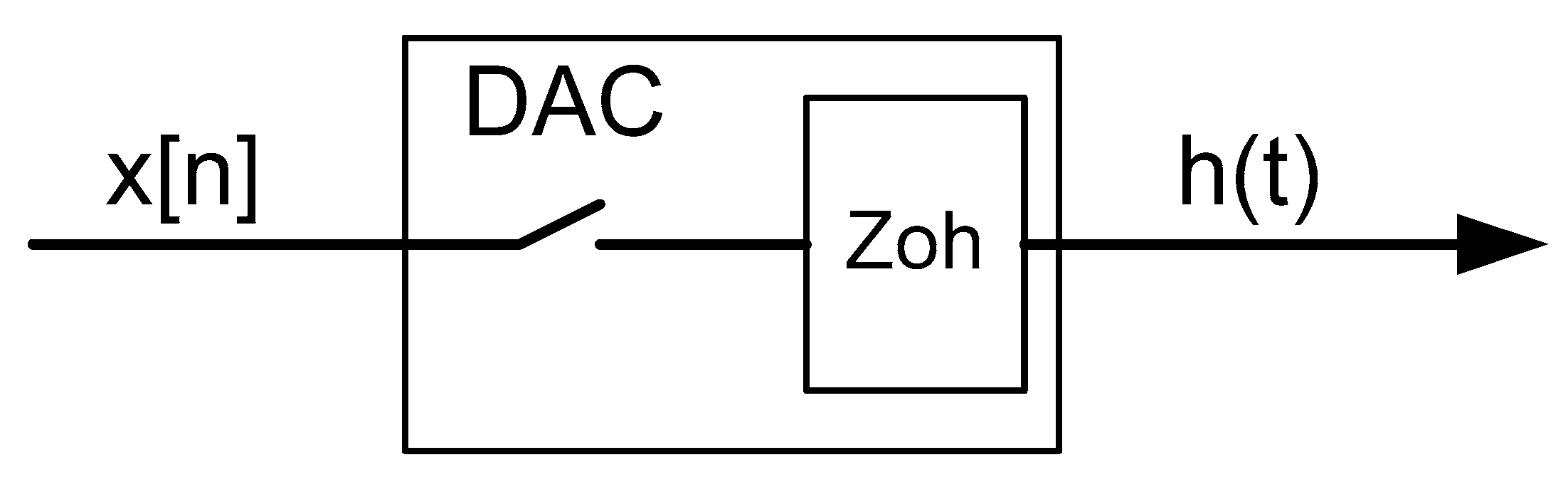
10.1. Zoh Mathematical Treatment
10.2. Applying Previous Results to Closed Loop
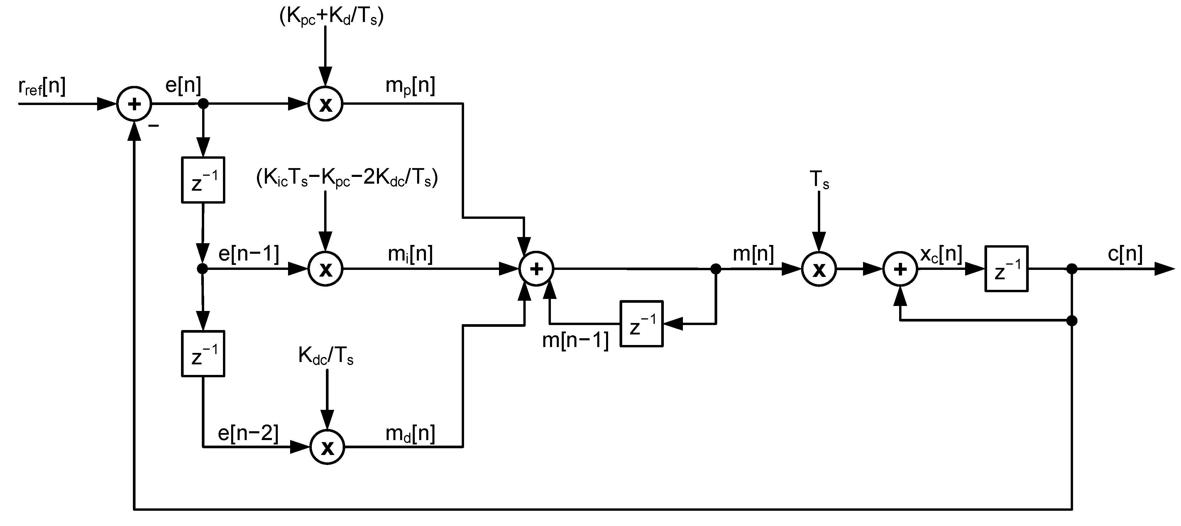
10.3. Analyzing Closed Loop with Velocity Form
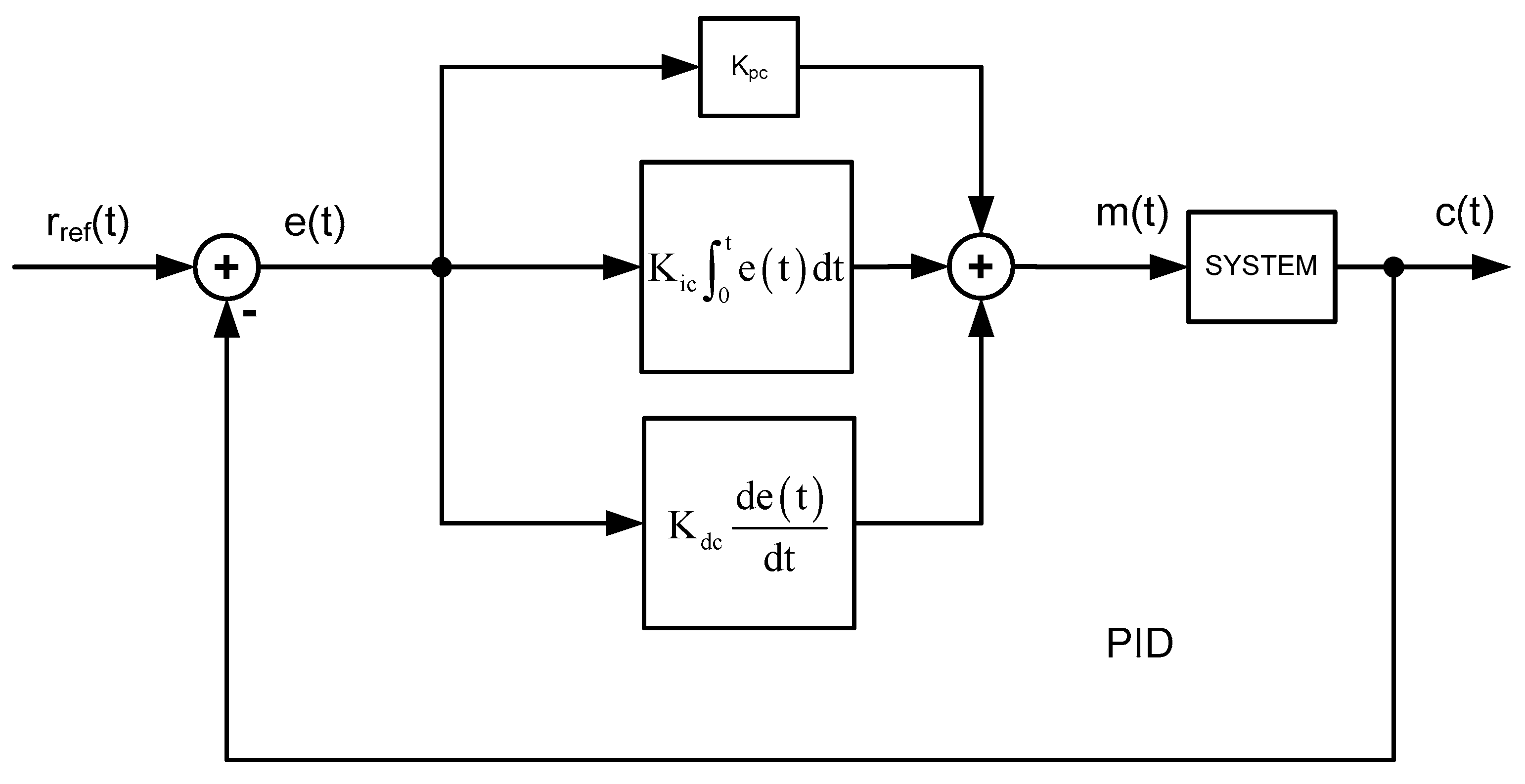
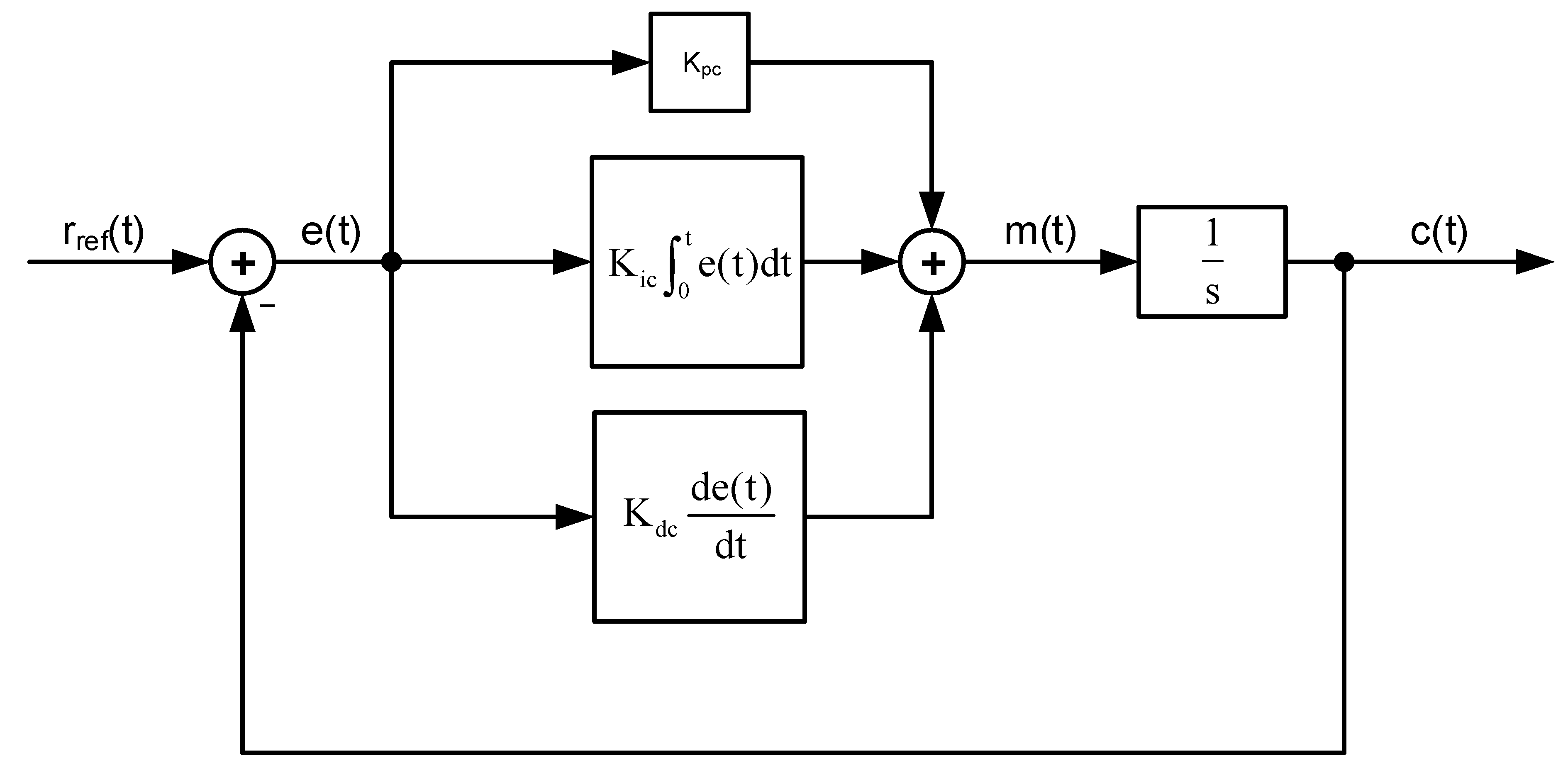
10.4. Fully Analog PID Loop Equations
11. Results
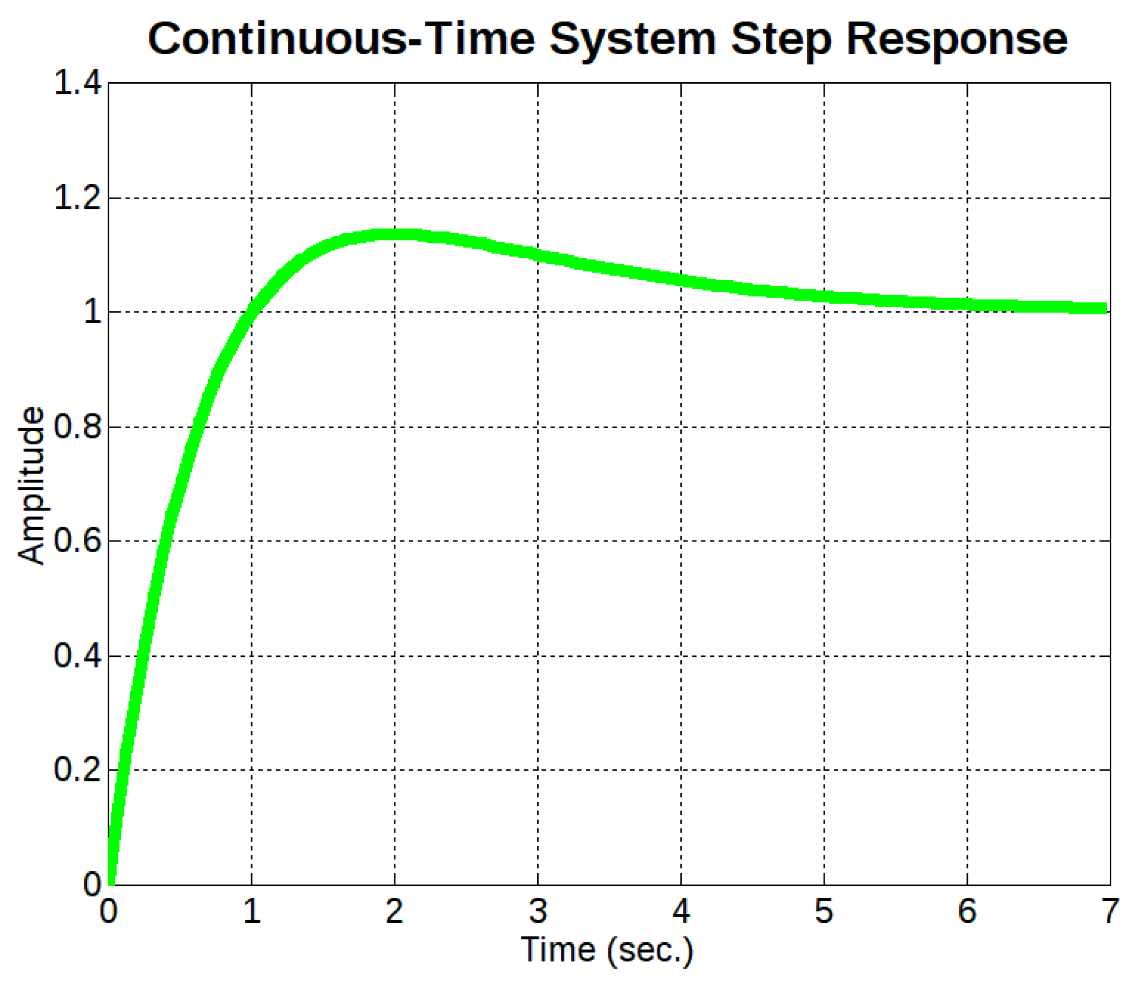
11.1. Continuous-Time System Response
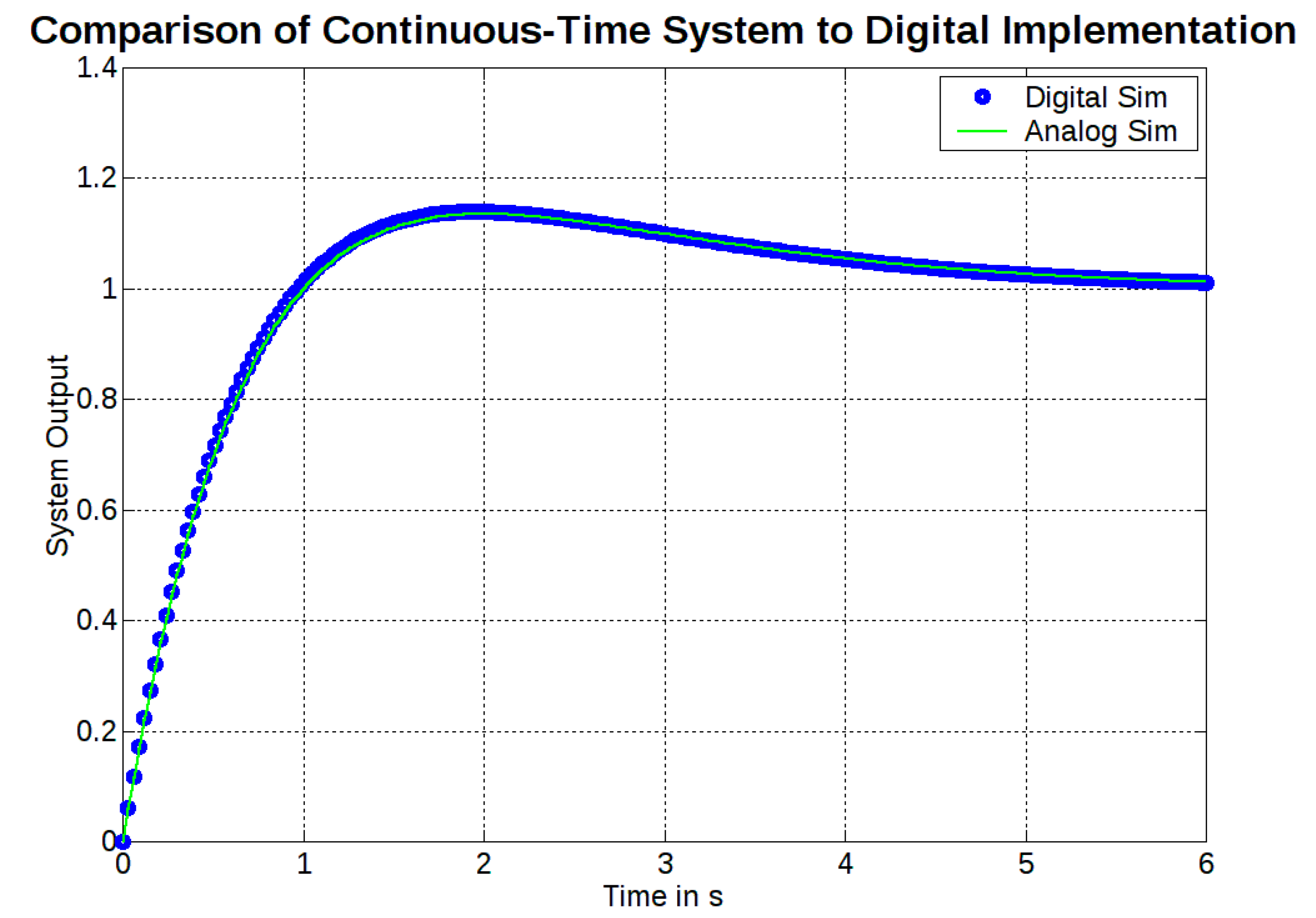
11.2. Discrete-Time System Response with Positional Form PID
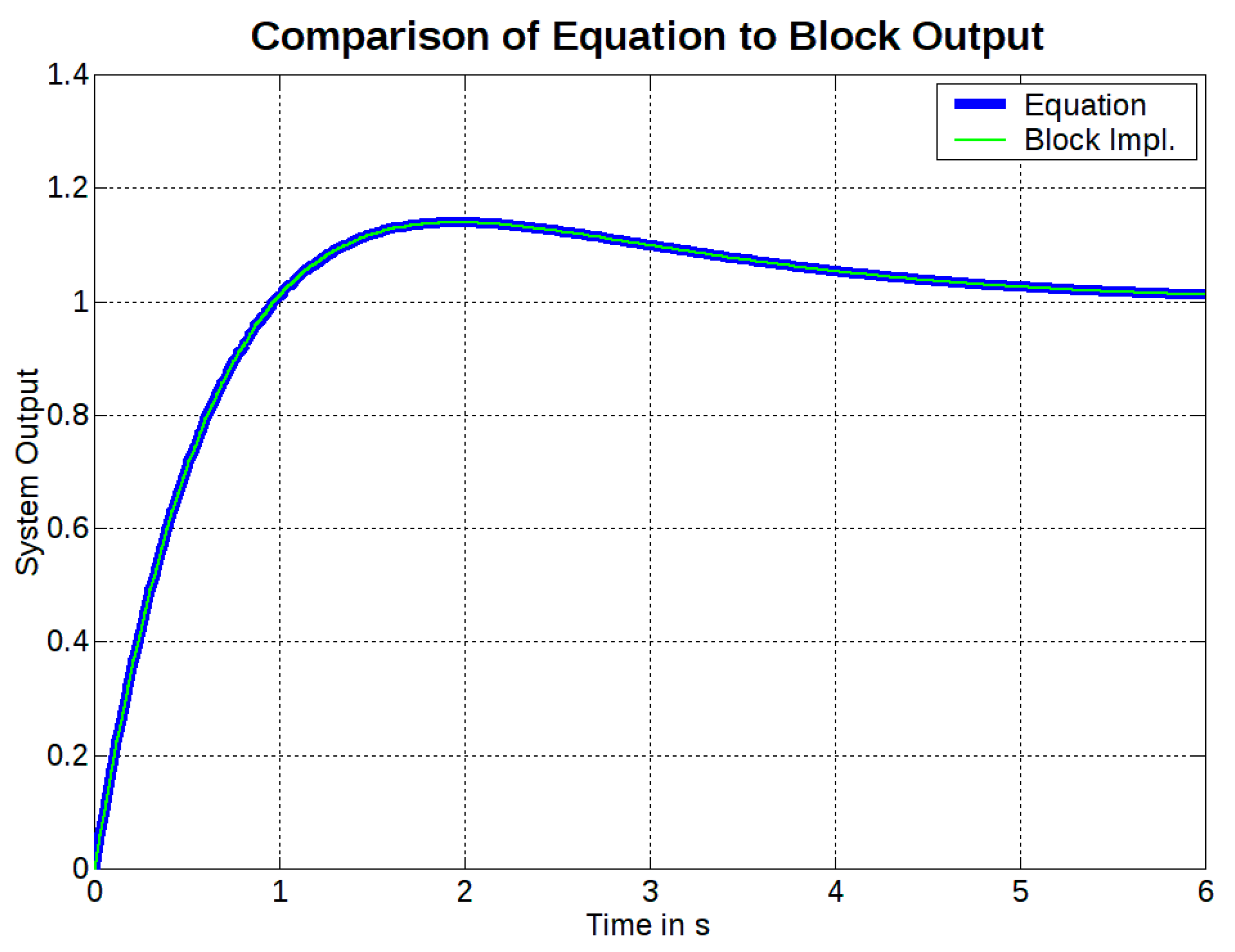
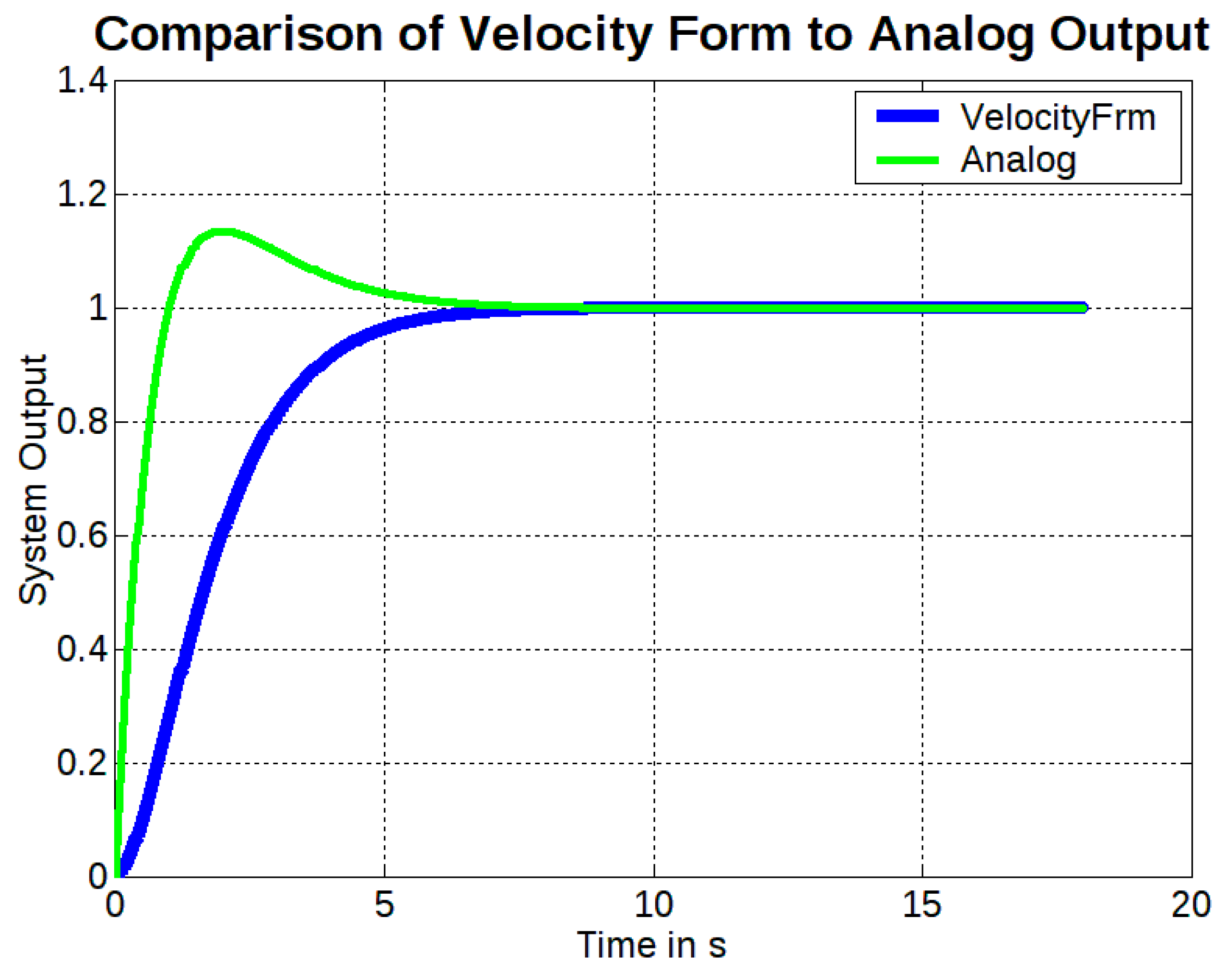
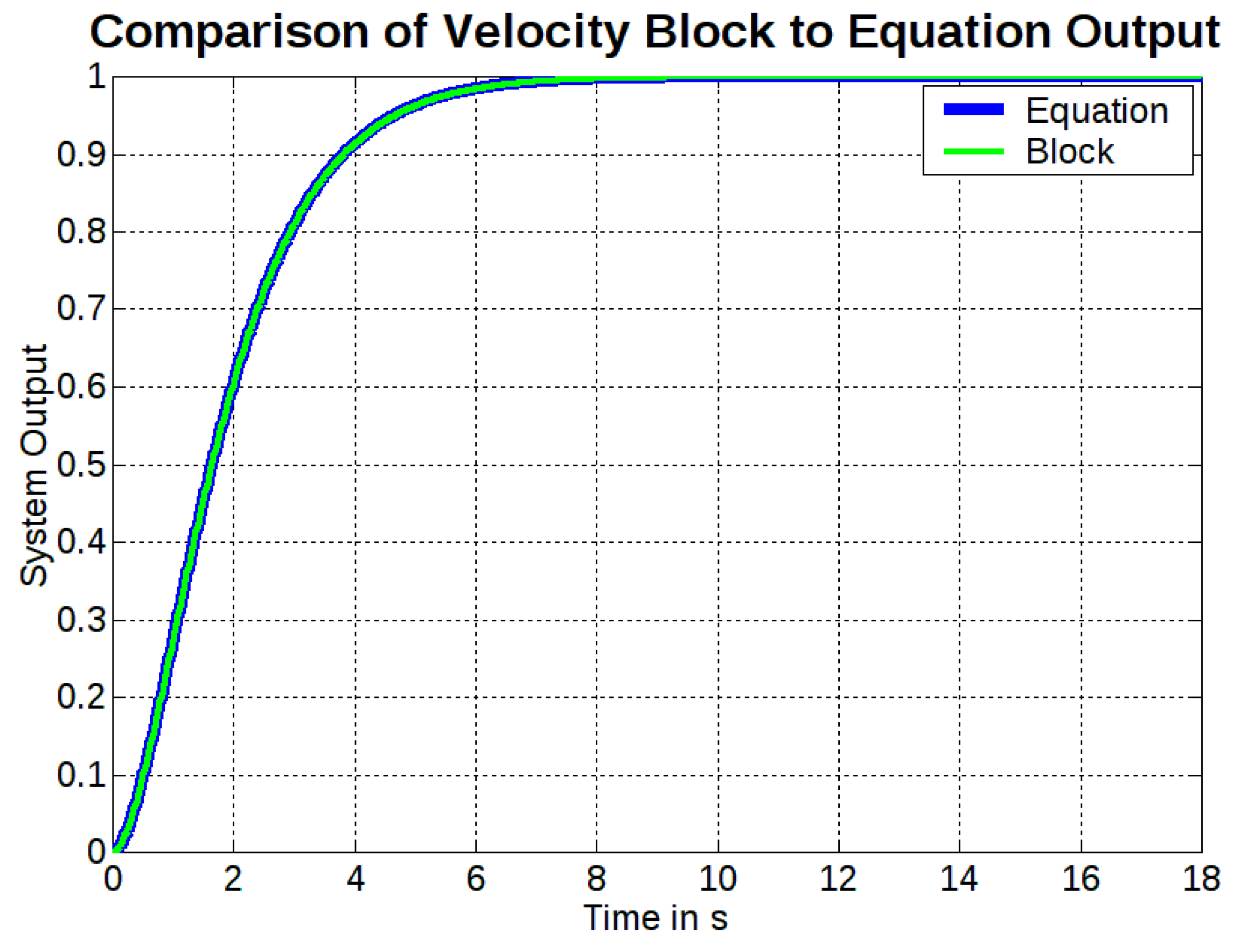
11.3. Discrete-Time System Response with Velocity Velocity Form PID
12. Analysis of Results and Discussion
13. Conclusions
Author Contributions
Funding
Institutional Review Board Statement
Informed Consent Statement
Data Availability Statement
Acknowledgments
Conflicts of Interest
Appendix A. Electric Propulsion System for Unmanned Craft


References
- Ogata, K. Discrete-Time Control Systems, 2nd ed.; Prentice-Hall Inc.: Englewood Cliffs, NJ, USA, 1995; ISBN 0-13-328642-8. [Google Scholar]
- Kuo, B.C. Digital Control Systems, 1st ed.; CBS Publishing Asia LTD: Hong Kong, 1987; ISBN 4-8337-0013-1. [Google Scholar]
- Bulten, N.W.H. Numerical Analysis of a Waterjet Propulsion System. Ph.D. Thesis, Eindhoven University of Technology, Eindhoven, The Netherlands, 2006. [Google Scholar]
- Xiros, N.; Loghis, E. System Identification Using Neural Nets for Dynamic Modeling of a Surface Marine Vehicle. In Proceedings of the ASME 2014 International Mechanical Engineering Congress and Exposition, Montreal, QC, Canada, 14–20 November 2014; p. V010T13A015. Available online: https://www.researchgate.net/publication/304221905_System_Identification_Using_Neural_Nets_for_Dynamic_Modeling_of_a_Surface_Marine_Vehicle/citation/download (accessed on 30 August 2022).
- Xiros, N.I.; Loghis, E.K. Continuous and Discrete-Time Models of Surface Watercraft Nonlinear Dynamics. Acta Sci. Comput. Sci. 2022, 4, 15–27. [Google Scholar]
- Papoulis, A. Signal Analysis, 1st ed.; McGraw-Hill: New York, NY, USA, 1984; ISBN 0-07-066468-4. [Google Scholar]
- Nagrath, I.J.; Gopal, M. Control Systems Engineering, 2nd ed.; John Wiley & Sons: Singapore, 1986; ISBN 9971-5-1056-1. [Google Scholar]
- Golnaraghi, F.; Kuo, B.C. Automatic Control Systems, 10th ed.; Wiley: Hoboken, NJ, USA, 2010; ISBN 978-0-470-04896-2. [Google Scholar]
- Xiros, N.I. Robust Control of Diesel Ship Propulsion, 1st ed.; Springer London: London, UK, 2002; ISBN 978-1-4471-0191-8. [Google Scholar]
- Xiros, N.I.; An, P.-C.E. Control Theory and Applications. In Springer Handbook of Ocean Engineering; Dhanak, M.R., Xiros, N.I., Eds.; Springer International Publishing: Cham, Switzerland, 2016; pp. 227–276. ISBN 978-3-319-16649-0. [Google Scholar]
- Xiros, N.I. Digital Signal Processing. In Springer Handbook of Ocean Engineering; Dhanak, M.R., Xiros, N.I., Eds.; Springer International Publishing: Cham, Switzerland, 2016; pp. 197–226. ISBN 978-3-319-16649-0. [Google Scholar]
- Oppenheim, A.V.; Schafer, R.W. Discrete-Time Signal Processing, 1st ed.; Prentice-Hall Inc.: Hoboken, NJ, USA, 1989; ISBN 0-13-216771-9. [Google Scholar]
- Soliman, S.S.; Srinath, M.D. Continuous and Discrete Signals and Systems, 2nd ed.; Prentice-Hall Inc.: Hoboken, NJ, USA, 1998; ISBN 0-13-569112-5. [Google Scholar]
- Fossen, T. Guidance and Control of Ocean Vehicles, 1st ed.; Wiley: Chicester, UK, 1994; ISBN 0-471-94113-1. [Google Scholar]
- Alciatore, D.G.; Histand, M.B. Introduction to Mechatronics and Measurement Systems, 4th ed.; McGraw-Hill: New York, NY, USA, 2012; ISBN 978-0-07-338023-0. [Google Scholar]
- Kilian, C.T. Modern Control Technology: Components and Systems, 3rd ed.; CENGAGE Delmar Learning: Clifton Park, NY, USA, 2005; ISBN 978-1-4018-5806-3. [Google Scholar]
- Auslander, D.M.; Kempf, C.J. Mechatronics: Mechanical System Interfacing, 1st ed.; Prentice Hall: Hoboken, NJ, USA, 1995; ISBN 978-0-13-120338-9. [Google Scholar]


Publisher’s Note: MDPI stays neutral with regard to jurisdictional claims in published maps and institutional affiliations. |
© 2022 by the authors. Licensee MDPI, Basel, Switzerland. This article is an open access article distributed under the terms and conditions of the Creative Commons Attribution (CC BY) license (https://creativecommons.org/licenses/by/4.0/).
Share and Cite
Loghis, E.K.; Xiros, N.I. Development of Discrete-Time Waterjet Control Systems Used in Surface Vehicle Thrust Vectoring. J. Mar. Sci. Eng. 2022, 10, 1844. https://doi.org/10.3390/jmse10121844
Loghis EK, Xiros NI. Development of Discrete-Time Waterjet Control Systems Used in Surface Vehicle Thrust Vectoring. Journal of Marine Science and Engineering. 2022; 10(12):1844. https://doi.org/10.3390/jmse10121844
Chicago/Turabian StyleLoghis, Eleftherios K., and Nikolaos I. Xiros. 2022. "Development of Discrete-Time Waterjet Control Systems Used in Surface Vehicle Thrust Vectoring" Journal of Marine Science and Engineering 10, no. 12: 1844. https://doi.org/10.3390/jmse10121844
APA StyleLoghis, E. K., & Xiros, N. I. (2022). Development of Discrete-Time Waterjet Control Systems Used in Surface Vehicle Thrust Vectoring. Journal of Marine Science and Engineering, 10(12), 1844. https://doi.org/10.3390/jmse10121844