Article

Circulation and Transport Processes during an Extreme Freshwater Discharge Event at the Tagus Estuary

1
Physics Department, University of Aveiro, Campus de Santiago, 3810-193 Aveiro, Portugal
2
CESAM, Centre for Environmental and Marine Studies, Physics Department, University of Aveiro, Campus de Santiago, 3810-193 Aveiro, Portugal
*
Author to whom correspondence should be addressed.
J. Mar. Sci. Eng. 2022, 10(10), 1410; https://doi.org/10.3390/jmse10101410
Submission received: 10 August 2022 / Revised: 23 September 2022 / Accepted: 24 September 2022 / Published: 2 October 2022
(This article belongs to the Special Issue Hydrodynamics and Mixing Processes in Estuaries and Lagoons)

Abstract

:
During the winter of 2013, the Tagus estuary was under the influence of intense winds and extreme freshwater discharge that changed its hydrodynamics and, consequently, the salt and heat transport. Moreover, the dynamics of the estuary may change due to climate change which will increase the frequency of heat waves and increase the mean sea level. Therefore, it is of utmost importance to study the impact of the future increase in air temperature and mean sea level under extreme events, such as that in the winter of 2013, to ascertain the foreseen changes in water properties transport within the estuary and near coastal zone. Several scenarios were developed and explored, using the Delft3D model suite, considering the results of the CMIP6 report as forcing conditions. Before the event, the mixing region of the estuary presented well-mixed conditions and its marine area a slight stratification. During the event, the estuary was filled with freshwater and the mixing region migrated toward the coast, leading to lower water temperature values inside the estuary. SLR has a higher impact on the salinity and stratification patterns than the air temperature increase. The response of water temperature is directly related to the increase in air temperature. The estuary mouth and the shallow regions will be more prone to changes than the upstream region of the estuary. The projected changes are directly linked to the future CO2 emissions scenarios, being intensive with the highest emission scenario.

1. Introduction

Climate change encompasses a significant alteration in the statistical values of meteoceanographic variables, over periods ranging from decades to longer time scales. These modifications may induce changes in the average conditions and in the occurrence of extreme events (for example, increases in the average air temperature and frequency of extreme events).
Estuaries are one of the marine systems that are subjected to major pressures. The connection between estuarine systems dynamics and climate change is clear [1,2,3], mostly due to anthropogenic activities, which are one of the pressures that induce global warming, exacerbating the response of these systems to the mean sea level rise [3,4,5,6,7]. Future projections [7] show that air temperature is increasing, impacting water temperature and salinity stratification in coastal regions [8,9], and affecting nutrient fluxes and the phytoplankton dynamics [10,11,12]. These coastal system dynamics depend on other forcings such as wind and freshwater discharge, which can largely impact the estuary dynamics [13], turning these regions into vulnerable systems and requesting frequent monitorization to control risks and associated damages.
The Tagus estuary is a coastal plain estuary located in the central region of Portugal, near the metropolitan area of Lisbon. It is a densely populated region subjected to enormous natural and human stress. It is situated in the eastern North Atlantic system, one of the main coastal upwelling systems, holds high productivity and biodiversity, acts as a nursery for fish species, and sheltes for vessels and harbor industries [14,15]. Salt marshes are considered to be the most productive ecosystems which provide feeding and sheltering to biodiversity; in addition, they act as sinks for contaminants and carbon. Salt marshes are susceptible to sea level rise, which may change the erosion rate and consequently affect the salt marshes. The temperature is also one of the limiting factors of salt marshes. It is the most critical driver limiting aquaculture because a species only tolerates a limited range of environmental conditions. The freshwater inflow can drastically change the salinity, which could impact the salt marshes, aquaculture, and the ship navigation on the Tagus estuary by affecting the ship’s buoyancy and flotation. Due to their ecological and economic value, it is necessary to study the current behavior of the estuary and assess future conditions and possible effects of climate change.
Between 20 March and 11 April of 2013, the region surrounding the Tagus River was influenced by intense southern winds [13].
During the event, the river flow reached 8711 m3/s, and the mean daily value over three consecutive days attained 7500 m3/s [16]. This led to an abrupt decrease in salinity values within the estuary. As mentioned by Vaz et al. [13], when the river inflow is high (higher than 1000 m3/s), the freshwater discharge enhances estuarine ebb velocities, promoting the propagation of low-salinity estuarine water toward the shelf. Similarly, the influence of intense southern winds induces a strong alongshore propagation of the Tagus plume, intensifying the poleward current [13].
A higher frequency of extreme events is expected in the future due to climate change, such as hazardous storms and intense precipitation, or heat and cold waves, making studying these events crucial to improve the global understanding of coastal lagoons’ response to global change [3,4,7]. Sea level rise (SLR), water temperature changes, variations in circulation patterns and frequency, and severity of extreme events will impact marine ecosystems [15]. The analysis of these systems’ vulnerabilities in a climate change scenario allows the establishment of mitigation and adaptation procedures to obtain the proper management and protection of such vulnerable ecosystems.
The numerical model predictions are beneficial to increase knowledge on expected climate change impacts and support decision making. Numerical models are suitable tools to reproduce climate change trends with enough accuracy to provide results that would be rather difficult to obtain through surveys [15].
Hereupon, this work aims to study the circulation and transport processes during the extreme hazardous event that occurred in the winter of 2013 in the Tagus estuary, in response to climate change drivers through a modeling study. The climate change drivers, such as the expected mean sea level rise, air temperature, and river discharges, are based on the shared socioeconomic pathways (SSPs) 2.6 and 8.5 from Coupled Model Intercomparison Project 6 (CMIP6). These meteoceanographic variables are analyzed to study the influence of the stratification and circulation patterns inside the Tagus estuary under extreme events.

2. Study Area

The Tagus estuary (Figure 1) is located in the central region of the Portuguese west coast and it is the largest estuary in the Iberian Peninsula [17]. It is divided into three distinct regions: the Tagus River mouth, the inner estuarine area, and the adjacent coastal zone [18]. These regions are connected and interact between one another. The complex geomorphology of the estuary is composed of a long and narrow channel (the Tagus corridor) connecting the Atlantic Ocean to a shallow inner region with tidal flats and salt marsh areas (the Mar da Palha region) [17]. The width varies between 2 km in the corridor channel and 17 km in the Mar da Palha [19]. The central area of the estuary presents depths from 0 m to 12 m, while the corridor is deeper, with depths of about 25–30 m.
The Tagus estuary acts as the interface between the coastal sea and the main affluent of this system, the Tagus River, which has a total length of approximately 1000 km and discharges an average flow of about 12,500 hm3/year (about 300 m3/s) [20,21]. Although on a smaller scale, the Sorraia Trancão Rivers are also relevant to the freshwater inflow into the estuary [22]. Moreover, the Tagus River basin contributes to the estuary turbidity with a high sedimentary influx of about 1–5 × 10⁶ metric tons/year [23].
The tide in the estuary is predominantly semidiurnal. The system is mesotidal, with a tidal range at the coast between 0.55 m and 3.86 m [24], being intensified along the estuary as a result of an estuarine resonance mode with a period of close to twelve hours, due to the estuary length, which enhances the M2 constituent [19,25,26]. The tidal range increases by 12% at 14 km upstream and 30% at 36 km upstream. The mean tidal prism is about 7.5 × 10⁸ m3, and the average freshwater volume entering the estuary, during a tidal cycle is 2% of the tidal prism [17,19], revealing the importance of tidal propagation in the estuarine circulation. Generally, the estuary is considered well-mixed, although it is possible to identify stratification at different periods of the tidal cycle, especially under high river flow and low tidal ranges scenarios [27,28]. The vertical stratification is induced by heat and salt advection, caused by the interaction between tides and river inflow and by heat exchanges between the estuary and atmosphere [17].
The local wind is an essential driver of circulation inside the estuary. Simultaneously with freshwater discharge, wind stress determines residual currents, which can lead to distinct transport pathways [29]. During the winter, wind circulation has predominant directions from the northwest, north, and southeast and ranges from 1.5 m/s to 14 m/s. During the spring, the predominant winds are from the north or the northwest and range from 1 m/s to 15 m/s [13].

3. Materials and Methods

3.1. Data

The main source of errors in numerical simulations arises from flaws in the quality of the data inputs [15,30]; therefore, data from different databases were used in this study to assure the best possible data quality.
The hydrodynamic model’s performance is highly influenced by the accuracy of the bathymetric data [30]. Here, the numerical bathymetry was generated using a combination of bathymetric data provided by different sources: the General Bathymetric Chart of the Oceans (GEBCO)—https://www.gebco.net/ (accessed on 1 September 2021); Light Detection and Ranging (LIDAR) data; samples obtained in Portuguese Hydrographic Institute (Instituto Hidrográfico (IH) http://www.hidrografico.pt/ (accessed on 1 September 2021)) (compilation of data surveys collected between 1964 and 2009).
Two types of tidal data were used in the model implementation: one for the open boundary forcing and the other for the model validation. The tidal data imposed on the model as a boundary condition were obtained from the TOPEX/POSEIDON and are based on a global ocean tidal model [31], representing the major 13 tidal harmonic constants (M2, S2, N2, K2, K1, O1, P1, Q1, MF, MM, M4, MS4, and MN4) with a spatial resolution of 0.083°. For the validation, water level data from December 2012 were used with a time step of 5 min. They were obtained from five tidal stations along the estuary (Figure 1).
As a landward boundary condition, freshwater discharge of the Tagus River was used. These data were obtained from the Sistema Nacional de Informação de Recursos Hídricos (SNIRH). Daily data were used for the spin-up period, while for the extreme event analysis, a time series of hourly data was used. The Sorraia River basin contributes nearly 8% of the Tagus River basin, and it was established that the Sorraia River discharge is 8% of the Tagus River freshwater discharge due to the lack of in situ data. The same procedure was adopted for the Trancão River, assuming its flow is 1% of the Tagus River [32].
Regarding salinity and water temperature, daily results from the Atlantic Iberian Biscay Irish Ocean model provided by Copernicus Marine Environment Monitoring Service (CMEMS—https://marine.copernicus.eu/ (accessed on 1 September 2021)) were used as open ocean boundary conditions. For model validation, data were obtained from a buoy located in the central region of the estuary (see Figure 1). This buoy holds an Acoustic Doppler Current Profiler (ADCP) at a depth of 1.8 m and multiparametric probes at a depth of 1 m. It records marine and atmospheric variables, such as air and water temperature, wind speed and direction, atmospheric pressure, salinity, and radiation, every 20 min [19]. These data were acquired between June 2012 and January 2017 and used to evaluate the model accuracy in reproducing transport conditions in the inner side of the estuary.
The meteorological data for surface boundary conditions were obtained from the Era-Interim global reanalysis from the ECMWF (European Center for Medium-Range Weather Forecasts). The variables used were the 10-meter zonal, meridional wind components, 2-meter air temperature and dew-point temperature, surface pressure, surface net solar radiation, and downward surface thermal radiation, with a temporal resolution of 3 h and a spatial resolution of 0.125°.

3.2. Numerical Model

Numerical models are the most suitable tools to represent the realistic evolution trends of coastal systems [15]. The Delft3D-FLOW model [33] was used to study hydrodynamics, which is one of the modules of the open-source model suite developed by WL|Delft Hydraulics in cooperation with the Delft University of Technology.

3.2.1. Model Implementation

The curvilinear grid (Figure 2) used in this work results from an adaptation of the one developed by Ribeiro [34], to include intertidal regions. This grid covers an area from approximately 38° N to 39° N and from 8.8° W to 9.5° W. The spatial resolution ranges from 120 m, in the inner estuary, to 1300 m, near the ocean boundary, with a mean resolution value of 380 m. This grid comprises a total number of 9069 cells. A spin-up period of 2 months was considered since, according to Braunschweig et al. [35], the spin-up period needs to be at least 2 times the estuary’s residence time. Following the Courant–Friedrichs–Lewy number [33], the time step was 30 s to achieve the stability of the model.
The tidal propagation was calibrated through the adjustment of bottom roughness, which assumes the depth-dependent Manning coefficient [34]. The Manning coefficients were adjusted considering that an increase in the bottom friction would decrease the tidal wave amplitude in that zone of the channel and the channel’s upstream. Moreover, an increase in the bottom roughness would increase the phase lag for high tide and a decrease for low tide [36].
Three freshwater points were also defined as outflows representing the Tagus, Sorraia, and Trancão Rivers. The final modeling configurations of the implementation developed are presented in Table 1.

3.2.2. Model Validation

The model implementation was previously calibrated and validated [34]. However, the calibration and validation were performed due to the numerical grid adaptation for this work. The model accuracy was evaluated through the Root Mean Square Error (RMSE) and its relative error (∆E) (Table 2) [37,38] between the observed and simulated tidal amplitude and phase of tidal constituents and the observed and simulated water temperature and salinity.
The stations of Alcochete (S), Lisboa (R), and Cascais (P) show the best results, with RMSE of 0.14, 0.10, and 0.07 m, respectively, and a Skill of 0.99. Similarly, the ∆E is lower than 5% for these stations. Regarding Vila Franca de Xira (T), the RMSE and Skill also represent a good fit between the model and observations, with ∆E slightly higher than 5%. Paço de Arcos (Q) shows the highest RMSE and ∆E disagreement, with 40 cm and ∆E of 16%, respectively, which may be explained by the time lag between the bathymetry and the tidal observational data. These results are in agreement with previous studies at the Tagus estuary [39] and other similar systems [40,41]. The model’s accuracy correctly predicts the spring-neap cycle.
The salinity and water temperature results were also validated using buoy measurements, and the statistical parameters are presented in Table 3.
The water temperature RMSE shows lower values (<0.5 °C) compared to Ribeiro et al. [34], whereas salinity RMSE results are slightly higher (1.68). Skill values are comparably low due to the small variability within the data, even if the RMSE indicates a good model fit. Generally, the model accurately reproduces the water temperature and salinity in the Tagus estuary. These results show that this model implementation can be applied to simulate reliable future conditions in the Tagus estuary.

3.3. Model Scenarios

The effect of climate change on Tagus estuary hydrodynamics and hydrography was assessed by considering four scenarios under extreme freshwater discharge (Table 4). These scenarios intend to understand the influence of the increase in air temperature and sea level separately and by combining both. Two scenarios were designed based on the CMIP6 presented by IPCC, considering the SSP1-2.6—low greenhouse gas (GHG) emissions and SSP5-8.5—high-GHG scenarios. All scenarios used in this work are detailed in Table 4.
The scenarios #Sc1 to #Sc4 were compared with #ScRef, which corresponds to the model validation implementation, where SLR and air temperature remain unchanged.

4. Results

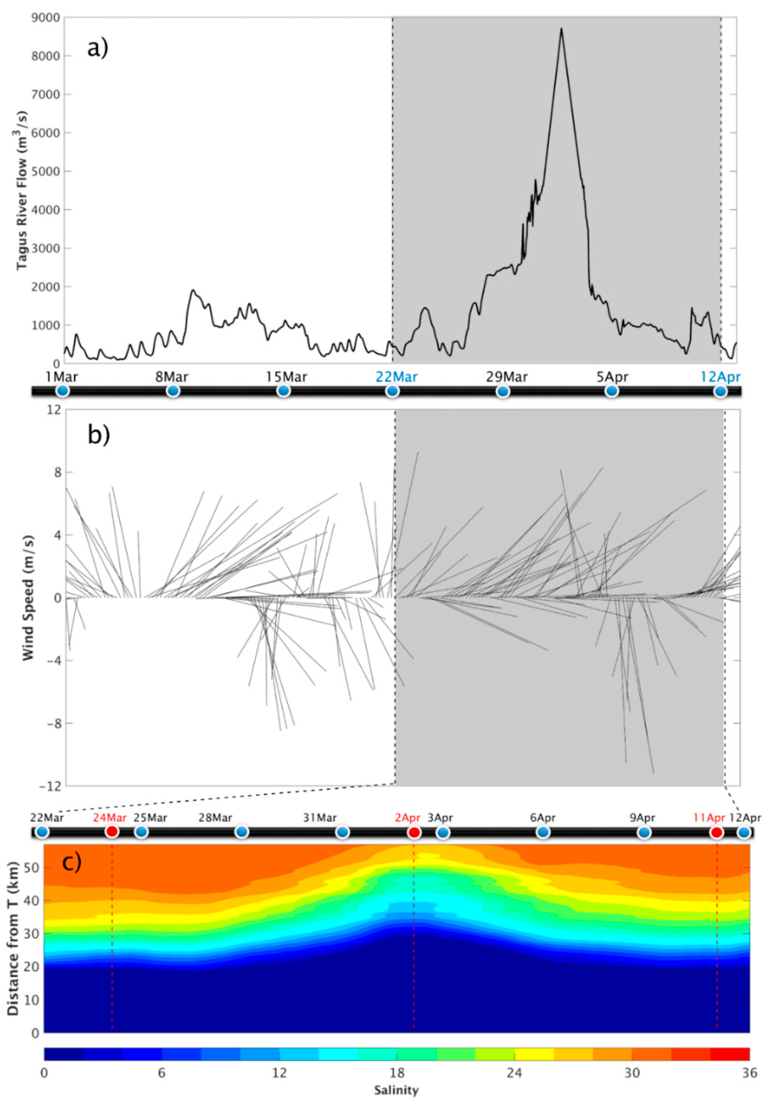
4.1. Event Characterization: 2013

The wind forcing and river discharge play an important role in the Tagus estuarine circulation. The salinity distribution during the event between 1 March and 13 April of 2013 will be characterized along the estuary under freshwater discharge and wind stress. Figure 3a,b show the Tagus River freshwater discharge and wind velocity, respectively, highlighting the period of 22 March to 12 April of 2013, which corresponds to peak (maximum) river discharge (1 April, value of 8711 m3/s).
The wind speed and direction are highly variable showing maximum values ranging from 8 to 12 m/s. The maximum discharge occurs when the wind blows from south–southwesterly. Before 22 March, the Tagus River discharge presented values between 1000 and 2000 m3/s, which are typical values for winter conditions. From this day forward, the river discharge increases, reaching peak values higher than 8000 m3/s in late March, remaining this discharge until 5 April. On this day, the wind changed its direction blowing from the north, changing the atmospheric conditions and promoting the conditions observed before the event.
The Tagus estuary average salinity evolution is depicted in Figure 3c. The results were filtered with a cut-off frequency of 33 h to remove tidal effects and inertial components [42]. Note that the filter may smooth the signal and, consequently, the salinity values.
The upstream region (10 km from T point) presents salinity values close to zero, while the estuary mouth shows values higher than thrity, except for the period between 31 March and 5 April. In this period, the central region of the estuary is dominated by freshwater, reaching salinity values of 28 outside the estuary. During typical conditions of freshwater inflow and wind, the mixing region is located between 20 and 45 km from the upstream region of the estuary, but after 28 March, this region migrated downstream.
The two-dimensional vertical salinity and water temperature patterns along the longitudinal section of the estuary (marked in Figure 1) were characterized using as proxies on three specific days: 24 March (before the extreme event); 2 April (during the event); 11 April (after the event). The vertical profiles along the longitudinal section were analyzed in terms of salinity (Figure 4), water temperature (Figure 5), and Brunt–Väisälä frequency (Figure 6) to assess the vertical stratification changes.
Before the extreme event (Figure 4a), the salinity profile reveals a well-mixed water column until 20 km from the Tagus River mouth (point T). In the mixing region, a stratified water column is visible up to 50 km from the river mouth, presenting surface values ranging from four to twenty-four between twenty and thirty kilometers from the upstream region. Between 30 and 45 km, the isohalines became steeper, with a maximum vertical salinity difference of eight. The water column became well-mixed in the estuary’s marine region with typical ocean salinity.
During the extreme freshwater event (Figure 4b), the water column is filled with freshwater (at the shallower region of the estuary), shifting the well-mixed region to 30 km from the T point, with a salinity close to zero. Surface values ranging from six to twenty-four and bottom values from eighteen to thirty-six are reached in the deeper region of the estuary. Between 30 and 50 km, top-to-bottom salinity differences of about 24 to 28 are visible. In the marine region of the estuary, a vertical salinity difference of about 18 is observed.
In Figure 4c, the salinity is around zero on the sector between the T point and the 20-kilometer mark. A stratified water column presents values ranging from six to eighteen between 20 and 30 km from point T. From this point forward, the isohalines became steeper, with a vertical salinity difference of eight. This difference decreased toward the marine region, where the water column started to be well-mixed again.
Figure 5 depicts the vertical water temperature structure along the estuary’s longitudinal section.
Before the extreme freshwater event (Figure 5a), the upstream region of the estuary (between 0 and 20 km) presents a well-mixed water column and a downstream gradient of 6 °C/20 km (0.3 °C/km). From this section to the ocean, a residual stratification occurs, with values around 16 °C, decreasing to 15 °C in the marine region of the estuary.
During the extreme freshwater event (Figure 5b), a well-mixed water column is visible at the inner region of the estuary (between 25 km from the Tagus River mouth). In the mixing region, vertical water temperature differences between 4 and 6 °C are observed, depicting the combined effect of heat transported by the river inflow and oceanic waters, respectively. The marine region’s water column is well-mixed in terms of temperature. During the event, a longitudinal gradient of 6 °C/50 km is visible along the estuary.
After the extreme freshwater event, the horizontal gradient decreases to 3.5 °C/50 km, decreasing the estuary’s stratification.
The evaluation of vertical stratification in the water column was also assessed by analyzing the Brunt–Väisälä frequency (N) (e.g., [43]) along the longitudinal section of the estuary. Smaller N values (lower than 60 cycles/h) indicate low stratification, whereas higher values (higher than 60 cycles/h) show higher stratification.
In the first 15 km from the T point (Figure 6a), N is low, with magnitudes between 0 and 20 cycles/h at the bottom, and 20 and 40 cycles/h at the surface, revealing well-mixed conditions throughout the water column. In the sector between 15 and 45 km from the T point, N increases significantly at the surface, reaching 180 cycles/h between 30 and 35 km, revealing a stratified water column. From the middle of the section toward the estuary mouth, the surface N are about two times higher than the bottom, which means that mixing increases on the bottom layers. At 50 km from point T, the water column stratifies, showing 100 cycles/h at the water column and 140 cycles/h at the surface. In the marine region, strong stratification is also visible, with values between 140 and 170 cycles/h along the water column and 70 cycles/h at the bottom, where mixing due to oceanic influence is visible.
Figure 6b presents an upstream pattern similar to that described for March 24, with values lower than 30 cycles/h in the first 25 km from point T. From 25 km to 30 km from point T, N reaches values between 80 and 140 cycles/h in all water columns, revealing strong stratification conditions. After 30 km from point T, surface N is higher than 140 cycles/h, reaching 180 cycles/h near the marine region. At the bottom, the values are about 100 cycles/h.
In the bottom panel (Figure 6c), N is lower than 50 cycles/h (mixed water column) in the first 20 km. After that, from 20 km to the end of the section, N varies between 70 and 120 cycles/h along the water column. At the bottom, N ranges from 40 to 80 cycles/h. A maximum N of 140 cycles/h is reached at the mixing region, decreasing in the remaining area.

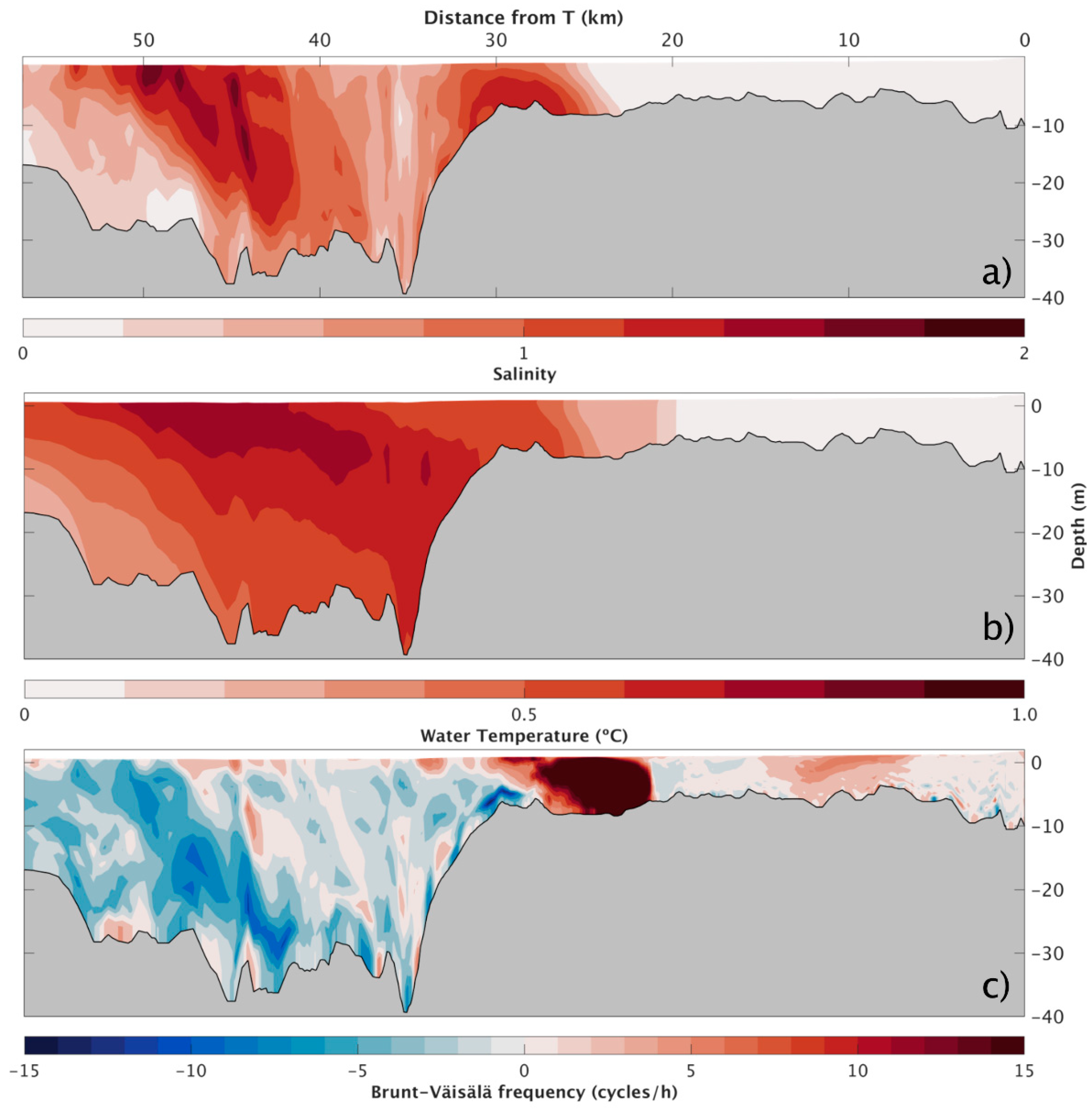
4.2. Changes in Water Properties Transport under a Climate Change Context

The effects of climate change on the water properties are assessed considering the climate drivers of air temperature and SLR by designing idealized climate change scenarios under extreme flow events. Two scenarios were designed considering each driver, #Sc1 for the air temperature and #Sc2 for the SLR. At the same time, the combined effects of these two variables are evaluated in #Sc3, considering the low-GHG emissions scenario, and #Sc4 for high-GHG emissions scenarios. The analysis was performed for 2 April (extreme freshwater event), and all scenarios were subsequently compared to the reference scenario (scenario minus the reference), meaning that positive values represent a variable increase and negative values a variable decrease.
Figure 7 considers the variations in vertical profiles of salinity, water temperature, and N along the longitudinal section of the estuary, from the reference scenario, under an air temperature increase (#Sc1).
In Figure 7a, for the first 30 km from the T point, the difference between #Sc1 and #ScRef is negligible. After that, the salinity increases reaching the maximum toward the estuary mouth, where a residual difference of 0.07 is observed at the bottom, revealing a salinity increase. The longitudinal water temperature structure presents a meager difference for #Sc1. Values lower than 0.2 °C are depicted in Figure 7b, and well-mixed conditions are visible. N differences (Figure 7c) are very low, with negligible values along most of the estuary, with some regions (upstream and in the estuary mouth) with maximum values of two cycles per hour. These results show that the increase of 1 °C in air temperature produces residual changes in estuarine water properties and stratification.
The estuary’s response to an SLR of 0.40 m (#Sc2) is evaluated (Figure 8) through the analyses of the vertical profiles of salinity, water temperature, and N along the longitudinal section of the estuary.
Near the estuary mouth, maxima salinity differences (about one) are observed at the surface and close to zero at the bottom. In the middle of the longitudinal section (mixing region of the estuary), salinity differences are around 0.8 near the bottom, presenting slightly higher values than the surface, where differences of ~0.5 are observed. The salinity differences are negligible in the initial 25 km from T point. These values reflect a slight increase in salinity compared to the reference scenario. Regarding water temperature, maximum differences of ~0.15 °C are reached in the central region of the section. In addition, SLR does not seem to influence the upstream area, where differences in water temperature are close to zero. In Figure 8c, N values are higher than in #Sc1. Stratification decreases along most of the longitudinal section, except between 20 and 30 km from T point, where values exceeding 20 cycles/h are observed, representing a slight increase in the stratification and a small decrease in mixing. Differences in salinity and water temperature are positive, showing an increase in these variables under future drivers.
Regarding stratification, the upper section of the estuary presents positive values of N, consistent with an increase in stratification due to SLR. Near the estuary mouth, negative values of N are observed, which is consistent with a decrease in stratification (mixing increases) due to higher values of mean sea level. A small fringe between 25 and 30 km shows a spot where the differences are higher, representing the formation of an estuarine front and impacting water properties and stratification patterns.
Figure 9 represents the variations in vertical profiles of salinity (Figure 9a), water temperature (Figure 9b), and N (Figure 9c) along the longitudinal section under a scenario of increasing air temperature (+1 °C) and SLR (+0.4 m) (#Sc3).
The salinity difference is higher in scenario #Sc3 (Figure 9a) compared with scenario #Sc1, with maximum values up to one. The salinity differences are negligible in the first 25 km from T point. In the section between 25 and 35 km, the salinity differences near the bottom are higher (about 0.8) than the surface (about 0.6), revealing a region where the main vertical features change abruptly, revealing the establishment of the estuarine front depicted in Figure 8a. From 35 km toward the ocean, salinity differences are higher on the surface (between 0.5 and 1) than at the bottom (>0.5). The salinity shows a maximum of about one at the surface in the section between 45 and 50 km from T point. Regarding water temperature (Figure 9b), a pattern similar to #Sc2 (Figure 8b) is observed, showing values around two times higher. The water temperature differences are close to zero in the first 20 km of the section. From 20 km to 35 km, differences of 0.25 °C are observed at the bottom and between 0.1 °C and 0.2 °C on the surface. From 35 km to the end of the longitudinal section, the surface water temperature differences go up to 0.3 °C and around 0.15 °C at the bottom. In Figure 9c, the N range is around four cycles per hour lower than those found in Figure 8c, but shows a similar pattern. The stratification decreases in most of the longitudinal section, except in a small fringe between 20 and 30 km from the T point, where values exceeding 15 cycles/h are observed (in the estuarine front region). Here, the stratification is expected to decrease (positive N), whereas the stratification should increase substantially for negative N.
An SLR of 0.7 m and an increase of 4.0 °C were considered to represent the high-GHG emissions scenario (#Sc4) (Figure 10).
Similar salinity patterns of #Sc3 are observed in scenario #Sc4 (Figure 10a), although with higher differences from the reference scenario (around 0.5). Salinity differences are around zero in the first 25 km from the T point. From 25 to 35 km, the differences near the bottom are higher (~1.2) than at the surface (about 0.8). From 35 km to the marine region, differences are higher on the surface (ranging from 0.5 to 2) than at the bottom (<1). Maxima values of two are found in a small region located around the surface, between 45 and 50 km from the T point. Figure 10b shows that the water temperature differences also present a similar pattern to those observed in the previous scenarios, but with differences greater than 0.4 °C, except in the upstream region (the first 20 km from the T point), where the differences are negligible. Between 20 and 30 km from the T point, the horizontal gradient is significant, with an increase of 0.5 °C. From 30 km to the marine region, differences at the bottom vary between 0.4 and 0.7 °C, while at the surface they vary from 0.7 to 0.9 °C, presenting a significant vertical gradient.
Concerning N (Figure 10c), in the regions where an increase in stratification was predicted (see #Sc3), the N difference is higher (~5 cycles/h). In regions where a decrease in N is observed, the mixing was intensified, showing higher magnitudes (5 cycles/h) compared with #Sc3. Compared with the reference scenario, the stratification decreases along the longitudinal section, except between 20 and 30 km from the T point, where values exceeding 15 cycles/h are observed.
The salinity Intrusion is quantified as the distance (in km) from the beginning of the longitudinal section (Figure 1b) to the isohaline 2 and was computed during the three stages of the extreme event for all scenarios (Figure 11a). Regarding the #ScRef, the salinity intrusion extends up to ~38 km before and after the event, while during the event it decreases to ~29 km. Comparing with the other scenarios, no significant differences were found when an increase in air temperature was considered (#Sc1 and #Sc3). Otherwise, the salinity intrusion increases approximately 1.5 km upstream with sea level rise (#Sc2 and #Sc4).
During the event, the vertical profiles of the water temperature (Figure 11b) and water column stability (Figure 11c) were analyzed regarding the salinity intrusion limit. The water temperature is proportional to the air temperature increase (up to 0.3 °C on the #Sc4), whereas the SLR driver is negligible (Figure 11b). The SLR was the driver that most influences the water column stability (Figure 11c), changing the pycnocline depth (where maximum N appears).

5. Discussion

The extreme event of freshwater discharge and persistent southern winds that occurred in 2013 altered the hydrographic features of the Tagus estuary and near coastal waters [44]. Under extreme freshwater discharge, the salinity and water temperature distribution changes significantly, with the fluvial region of the estuary being dominated by the freshwater (zero in salinity and typical riverine water temperature). This region became well-mixed due to the predominant freshwater, which affected the mixing region of the estuary by shifting this region toward the estuary mouth. In addition, strong stratification was visible from the mixing area to the estuary mouth during the event due to the freshwater discharge that boosted estuarine ebb velocities [13,45] at the surface. After the event, river inflow decreased to typical values, and the mixing region moved back to its previous position. The stratification observed during the event lost magnitude in these two regions [46].
The effects of future changes in sea level and water temperature on the estuary hydrographic features and stratification were also assessed by designing four scenarios. Scenario #Sc1 shows that an air temperature increase of 1 °C does not significantly impact the vertical patterns of salinity and N, except in regions dominated by freshwater. This influence tends to be larger in shallow areas, according to a similar study developed by Fortunato et al. [47], where mixing increases. This increase in the air temperature leads to a water temperature rise of 0.2 °C, i.e., about 25% of the air temperature change.
According to Mills et al. [48], the spatial distribution of salinity is highly dependent on bathymetry and, consequently, on the water column’s depth. Comparing to the previous scenario, the influence of SLR (#Sc2) on the water temperature is low, however, the salinity increased under a 0.40-meter rise in mean sea level. This pattern is not observed in the downstream zone of the estuary due to the increase in the water column, where seawater flows into the estuary. The SLR may also contribute to the stratification changes in specific regions along the estuary. As also observed by Hong and Shen [49], the SLR increases the pycnocline depth, indicating that the volume of the water is higher, and more saltwater enters the Tagus estuary. The increase in salinity also affects the estuary–coast interaction by reducing the estuary effect on the coast [50,51]. In general, the SLR significantly impacts vertical salinity and temperature patterns [47,48]. Comparing #Sc1 and#Sc2, SLR has a much higher impact than the air temperature on the vertical salinity and N patterns. On the other hand, the water temperature is more responsive to an increase in air temperature.
Regarding the #Sc3 scenario, the similarities between Figure 9a and Figure 8a and Figure 9c and Figure 8c are evident. As previously observed, the SLR increase (#Sc2) affects the salinity and N, and the water temperature depends mainly on the air temperature. The balance in both drivers intensifies the variables under study. In general, the increase in water temperature and salinity in the estuary occurs in the deeper regions.
The #Sc4 shows similar patterns to #Sc3. However, the values for the salinity, water temperature, and stratification will change according to the climate drivers of each scenario. The SLR has a higher impact than the air temperature on the salinity, water temperature, and N patterns since it boosts oceanic water transport into the estuary, which can change the region’s dynamics. Regarding the salinity, water temperature, and N patterns found along the longitudinal section of the estuary, these variables will not change their values along the first 20 km from the T point, with negligible differences found for all climate change scenarios. Here, the high freshwater discharge inhibits the impact of air temperature and SLR changes. From this point (20 km) forward, the salinity, water temperature, and vertical mixing will increase in response to the air temperature and the SLR under climate change scenarios. Rising sea levels lead to enhanced salinity intrusion at Tagus estuary, as found in other similar estuaries [45,52], however, the extreme discharge attenuates it. Similarly, the increase in air temperature induces an increase in water temperature, which may negatively impact the ecosystem. These impacts may be intensified by the combination of the increased salinity intrusion, water temperature, and extreme freshwater discharges.

6. Conclusions

The impact of future changes in the hydrographic patterns at the Tagus estuary induced by extreme events similar to the one that occurred in the winter of 2013 was studied. The impact of extreme discharges was also studied in a climate change context since the dynamics of the estuary may change in the future with an increase in the frequency of heat waves and mean SLR. A numerical model application using the Delft3D-Flow module was developed to reproduce the Tagus estuary’s tidal properties and salt and heat propagation. The changes induced by different scenarios representing the effects of climate changes in conditions of high freshwater discharges, air temperatures, and mean sea level were characterized, and the impact of changes on salinity, water temperature, and stratification patterns were evaluated.
For the reference scenario, vertically averaged salinity presented lower values (<1) than usual during the event, with a maximum (near the estuary mouth) around 24. Nine days later, some effects of the event are still noticed, as salinity values are lower than usual. The water temperature observed between 21 March and 11 April showed the typical patterns, with the warmer water in the intermediate zone of the longitudinal section (in the shallow region). While during the event, minima values were found in the estuary mouth, revealing that the influence of the riverine discharge induced low temperatures. The stratification in the estuary was also assessed using the Brunt–Väisälä frequency (N). In the region near the Tagus River mouth, N was low, i.e., this area is well-mixed. N increases substantially on the surface from the middle of the section to the estuary mouth. During the event, the stratification was higher in the entire water column. After that, mixing increased compared to before the event, according to the water temperature patterns.
The air temperature increase expected in a climate change context will induce a water temperature rise. However, it will not significantly impact the vertical patterns of salinity and N. The salinity and stratification will be affected by a 0.40-meter rise in mean sea level, except in the upstream region of the estuary. Similarly, the SLR will not have a significant impact on water temperature. Comparing #Sc1 and #Sc2, SLR will have a much higher impact than the air temperature increases in the vertical patterns of salinity and N. In opposition, the response of water temperature will be essentially promoted by the increase in the air temperature.
From the analysis of #Sc3 and #Sc4, it was observed that the SLR would act essentially on the salinity and N, while the air temperature changes will impact the water temperature. Moreover, the estuary mouth and the shallow areas will present more significant changes in the water temperature and salinity than the upstream region of the estuary (near the river mouth), where the river inflow is dominant in the establishment of salinity and water temperature patterns (the air temperature increase and SLR will not have considerable effects in this region).
Although the impact of SLR was higher than the air temperature increase, both are linked, which means that an air temperature increase will result in an SLR increase.
The projected changes will be greater for the scenario SSP5-8.5 and considerably smaller for SSP1-2.6. As referred to by Ferrero et al. [6], this enhances the importance of implementing public policies leading to lower emission scenarios. Thus, it is essential to increase the number of studies on the impact of climate change and improve their visibility among politicians, managers, stakeholders, and society. Thus, all efforts must be focused on reversing the cycle of the decline of ocean health and, consequently, estuarine systems’ decadence. The aim should be to ensure that ocean science supports countries in creating improved conditions for sustainable ocean development.

Author Contributions

Conceptualization: N.V. and M.S.; methodology: N.V. and M.S.; validation, A.F.R.; formal analysis, A.F.R., M.S. and N.V.; investigation, A.F.R.; writing—original draft preparation, A.F.R., M.S., N.V., A.P., A.S.R. and J.M.D.; writing—review and editing, A.F.R., M.S., N.V., A.P., A.S.R. and J.M.D.; visualization, A.F.R.; supervision, N.V. and M.S. All authors have read and agreed to the published version of the manuscript.

Funding

We acknowledge financial support to CESAM by FCT/MCTES (UIDP/50017/2020+UIDB/50017/2020+ LA/P/0094/2020) through national funds. Additionally, this study was partially supported under the SMART project funded by the AI Moonshot Challenge 2020, promoted by the Portuguese Space Agency—Portugal Space.

Institutional Review Board Statement

Not applicable.

Informed Consent Statement

Not applicable.

Data Availability Statement

Not applicable.

Conflicts of Interest

The authors declare no conflict of interest. The funders had no role in the design of the study; in the collection, analyses, or interpretation of data; in the writing of the manuscript; in the decision to publish the results.

References

  1. Chapman, P.M. Management of coastal lagoons under climate change. Estuar. Coast. Shelf Sci. 2012, 110, 32–35. [Google Scholar] [CrossRef]
  2. Statham, P.J. Nutrients in estuaries—An overview and the potential impacts of climate change. Sci. Total Environ. 2012, 434, 213–227. [Google Scholar] [CrossRef] [PubMed]
  3. Rodrigues, M.; Rosa, A.; Cravo, A.; Jacob, J.; Fortunato, A.B. Effects of climate change and anthropogenic pressures in the water quality of a coastal lagoon (Ria Formosa, Portugal). Sci. Total Environ. 2021, 780, 146311. [Google Scholar] [CrossRef] [PubMed]
  4. IPCC. Climate Change 2013: The Physical Science Basis. Contribution of Working Group I to the Fifth Assessment Report of the Intergovernmental Panel on Climate Change; Cambridge University Press: Cambridge, UK; New York, NY, USA, 2013.
  5. Rodrigues, M.; Oliveira, A.; Queiroga, H.; Brotas, V.; Fortunato, A.B. Modelling the effects of climate change in estuarine ecosystems with coupled hydrodynamic and biogeochemical models. In Developments in Environmental Modelling; Elsevier: Amsterdam, The Netherlands, 2015; Volume 27, pp. 271–288. [Google Scholar]
  6. Ferrero, B.; Tonelli, M.; Marcello, F.; Wainer, I. Long-term Regional Dynamic Sea Level Changes from CMIP6 Projections. Adv. Atmos. Sci. 2021, 38, 157–167. [Google Scholar] [CrossRef]
  7. IPCC. Climate Change 2021: The Physical Science Basis. Contribution of Working Group I to the Sixth Assessment Report of the Intergovernmental Panel on Climate Change; Cambridge University Press: Cambridge, UK; New York, NY, USA, 2021.
  8. De Pascalis, F.; Pérez-Ruzafa, A.; Gilabert, J.; Marcos, C.; Umgiesser, G. Climate change response of the Mar Menor coastal lagoon (Spain) using a hydrodynamic finite element model. Estuar. Coast. Shelf Sci. 2012, 114, 118–129. [Google Scholar] [CrossRef]
  9. Shalby, A.; Elshemy, M.; Zeidan, B.A. Modeling of climate change impacts on Lake Burullus, coastal lagoon (Egypt). Int. J. Sediment Res. 2021, 36, 756–769. [Google Scholar] [CrossRef]
  10. Brito, A.C.; Newton, A.; Tett, P.; Fernandes, T.F. How will shallow coastal lagoons respond to climate change? A modelling investigation. Estuar. Coast. Shelf Sci. 2012, 112, 98–104. [Google Scholar] [CrossRef]
  11. Lloret, J.; Marín, A.; Marín-Guirao, L. Is coastal lagoon eutrophication likely to be aggravated by global climate change? Estuar. Coast. Shelf Sci. 2008, 78, 403–412. [Google Scholar] [CrossRef]
  12. Pesce, M.; Critto, A.; Torresan, S.; Giubilato, E.; Pizzol, L.; Marcomini, A. Assessing uncertainty of hydrological and ecological parameters originating from the application of an ensemble of ten global-regional climate model projections in a coastal ecosystem of the lagoon of Venice, Italy. Ecol. Eng. 2019, 133, 121–136. [Google Scholar] [CrossRef]
  13. Vaz, N.; Rodrigues, J.G.; Mateus, M.; Franz, G.; Campuzano, F.; Neves, R.; Dias, J.M. Subtidal variability of the Tagus river plume in winter 2013. Sci. Total Environ. 2018, 627, 1353–1362. [Google Scholar] [CrossRef]
  14. Rodrigues, J. The Tagus Estuarine Plume Variability: Impact in Coastal Circulation and Hydrography. Master’s Thesis, University of Aveiro, Aveiro, Portugal, 2015. [Google Scholar]
  15. Des, M. Hydrodynamics of NW Iberian Peninsula under Past and Future Climate Hydrodynamics of NW Iberian Peninsula under Past and Future Climate Conditions Marisela Des Villanueva Mención Internacional. Ph.D. Thesis, Universidade de Vigo, Vigo, Spain, 2020. [Google Scholar]
  16. de Pablo, H.; Sobrinho, J.; Garcia, M.; Campuzano, F.; Juliano, M.; Neves, R. Validation of the 3D-MOHID hydrodynamic model for the Tagus coastal area. Water 2019, 11, 1713. [Google Scholar] [CrossRef] [Green Version]
  17. Vaz, N.; Mateus, M.; Pinto, L.; Neves, R.; Dias, J.M. The Tagus Estuary as a Numerical Modeling Test Bed: A Review. Geosciences 2020, 10, 4. [Google Scholar] [CrossRef] [Green Version]
  18. Vaz, N.; Dias, J.M. Hydrographic characterization of an estuarine tidal channel. J. Mar. Syst. 2008, 70, 168–181. [Google Scholar] [CrossRef]
  19. Franz, G.; Pinto, L.; Ascione, I.; Mateus, M.; Fernandes, R.; Leitão, P.; Neves, R. Modelling of cohesive sediment dynamics in tidal estuarine systems: Case study of Tagus estuary, Portugal. Estuar. Coast. Shelf Sci. 2014, 151, 34–44. [Google Scholar] [CrossRef]
  20. Portela, L.I.; Neves, R. Numerical modelling of suspended sediment transport in tidal estuaries: A comparison between the Tagus (Portugal) and the Scheldt (Belgium-The Netherlands). Netherl. J. Aquat. Ecol. 1994, 28, 329–335. [Google Scholar] [CrossRef]
  21. Lobanova, A.; Koch, H.; Liersch, S.; Hattermann, F.F.; Krysanova, V. Impacts of changing climate on the hydrology and hydropower production of the Tagus River basin. Hydrol. Process. 2016, 30, 5039–5052. [Google Scholar] [CrossRef]
  22. Rodrigues, R.; Cunha, R.; Rocha, F. Evaluation of river inflows to the Portuguese estuaries based on their duration curves. EMMA Proj. Rep. 2009, 40. [Google Scholar]
  23. Pinto, P.J.; Kondolf, G.M. Evolution of two urbanized estuaries: Environmental change, legal framework, and implications for sea-level rise vulnerability. Water 2016, 8, 535. [Google Scholar] [CrossRef] [Green Version]
  24. Guerreiro, M.; Fortunato, A.B.; Freire, P.; Rilo, A.; Taborda, R.; Freitas, M.C.; Andrade, C.; Silva, T.; Rodrigues, M.; Bertin, X.; et al. Evolution of the hydrodynamics of the Tagus estuary (Portugal) in the 21st century. J. Integr. Coast. Zo. Manag. 2015, 15, 65–80. [Google Scholar] [CrossRef]
  25. Fortunato, A.B.; Baptista, A.M.; Luettich Jr, R.A. A three-dimensional model of tidal currents in the mouth of the Tagus estuary. Cont. Shelf Res. 1997, 17, 1689–1714. [Google Scholar] [CrossRef]
  26. Fortunato, A.B.; Oliveira, A.; Baptista, A.M. On the effect of tidal flats on the hydrodynamics of the Tagus estuary. Oceanol. Acta 1999, 22, 31–44. [Google Scholar] [CrossRef]
  27. Rodrigues, M.; Fortunato, A.B. Assessment of a three-dimensional baroclinic circulation model of the Tagus estuary (Portugal). AIMS Environ. Sci. 2017, 4, 763–787. [Google Scholar] [CrossRef]
  28. Neves, F.S. Dynamics and Hydrology of the Tagus Estuary: Results from In Situ Observations. Ph.D. Thesis, University of Lisbon, Lisbon, Portugal, 2010. [Google Scholar]
  29. Vaz, N.; Dias, J.M. Residual currents and transport pathways in the Tagus estuary, Portugal: The role of freshwater discharge and wind. J. Coast. Res. 2014, 70, 610–625. [Google Scholar] [CrossRef]
  30. e Silva, J.D. Controls on Exchange in a Subtropical Tidal Embayment, Maputo Bay. Ph.D. Thesis, University of Wales, Bangor, Wales, 2007. [Google Scholar]
  31. Matsumoto, K.; Takanezawa, T.; Ooe, M. Ocean tide models developed by assimilating TOPEX/POSEIDON altimeter data into hydrodynamical model: A global model and a regional model around Japan. J. Oceanogr. 2000, 56, 567–581. [Google Scholar] [CrossRef]
  32. Lúcio, C.M.C. Análise do Comportamento Hidrológico da Bacia Hidrográfica do rio de Loures e Modelação da Sua Susceptibilidade a Cheias. Master’s Thesis, University of Lisbon, Lisbon, Portugal, 2014. [Google Scholar]
  33. Deltares. Delft3D-FLOW User Manual; Deltares: Delft, The Netherlands, 2021. [Google Scholar]
  34. Ribeiro, A.S. Coupled Modelling of the Tagus and Sado Estuaries and Their Associated Mesoscale Patterns. Master’s Thesis, University of Aveiro, Aveiro, Portugal, 2015. [Google Scholar]
  35. Braunschweig, F.; Martins, F.; Chambel, P.; Neves, R. A methodology to estimate renewal time scales in estuaries: The Tagus Estuary case. In Ocean Dynamics; Springer: Berlin, Germany, 2003; Volume 53, pp. 137–145. [Google Scholar]
  36. Fry, V.A.; Aubrey, D.G. Tidal velocity asymmetries and bedload transport in shallow embayments. Estuar. Coast. Shelf Sci. 1990, 30, 453–473. [Google Scholar] [CrossRef] [Green Version]
  37. Willmott, C.J. On the validation of models. Phys. Geogr. 1981, 2, 184–194. [Google Scholar] [CrossRef]
  38. Warner, J.C.; Geyer, W.R.; Lerczak, J.A. Numerical modeling of an estuary: A comprehensive skill assessment. J. Geophys. Res. Ocean. 2005, 110, C05001. [Google Scholar] [CrossRef]
  39. Dias, J.M.; Valentim, J.M.; Sousa, M.C. A numerical study of local variations in tidal regime of Tagus estuary, Portugal. PLoS ONE 2013, 8, e80540. [Google Scholar] [CrossRef] [Green Version]
  40. Picado, A.; Mendes, J.; Ruela, R.; Pinheiro, J.; Dias, J.M. Physico-chemical characterization of two portuguese coastal systems: Ria de Alvor and Mira estuary. J. Mar. Sci. Eng. 2020, 8, 537. [Google Scholar] [CrossRef]
  41. Dias, J.M.; Pereira, F.; Picado, A.; Lopes, C.L.; Pinheiro, J.P.; Lopes, S.M.; Pinho, P.G. A comprehensive estuarine hydrodynamics-salinity study: Impact of morphologic changes on Ria de Aveiro (atlantic coast of Portugal). J. Mar. Sci. Eng. 2021, 9, 234. [Google Scholar] [CrossRef]
  42. Otero, P.; Ruiz-Villarreal, M.; Peliz, A. Variability of river plumes off Northwest Iberia in response to wind events. J. Mar. Syst. 2008, 72, 238–255. [Google Scholar] [CrossRef]
  43. Prinsenberg, S.J.; Rattray, M., Jr. Effects of continental slope and variable Brunt-Väisälä frequency on the coastal generation of internal tides. Deep Sea Res. Oceanogr. Abstr. 1975, 22, 251–263. [Google Scholar] [CrossRef]
  44. Diário de Notícias Subida do rio coloca Bacia do Tejo em “alerta amarelo” 2013. Available online: https://www.dn.pt/portugal/sul/subida-do-rio-coloca-bacia-do-tejo-em-alerta-amarelo-3134341.html (accessed on 1 August 2021).
  45. Chua, V.P.; Xu, M. Impacts of sea-level rise on estuarine circulation: An idealized estuary and San Francisco Bay. J. Mar. Syst. 2014, 139, 58–67. [Google Scholar] [CrossRef]
  46. Losada, M.A.; Díez-Minguito, M.; Reyes-Merlo, M.Á. Tidal-fluvial interaction in the Guadalquivir Estuary: Spatial and frequency-dependent response of currents and water levels. J. Geophys. Res. Ocean. 2017, 122, 847–865. [Google Scholar]
  47. Fortunato, A.B.; Freire, P.; Mengual, B.; Bertin, X.; Pinto, C.; Martins, K.; Guérin, T.; Azevedo, A. Sediment dynamics and morphological evolution in the Tagus Estuary inlet. Mar. Geol. 2021, 440, 106590. [Google Scholar] [CrossRef]
  48. Mills, L.; Janeiro, J.; Martins, F. The Effects of Sea Level Rise on Salinity and Tidal Flooding Patterns in the Guadiana Estuary. In Proceedings of the International Conference on Sustainable Development of Water and Environment, Incheon, Korea, 13–14 January 2020; pp. 17–30. [Google Scholar]
  49. Hong, B.; Shen, J. Responses of estuarine salinity and transport processes to potential future sea-level rise in the Chesapeake Bay. Estuar. Coast. Shelf Sci. 2012, 104–105, 33–35. [Google Scholar] [CrossRef]
  50. Vaz, N.; Fernandes, L.; Leitão, P.C.; Dias, J.M.; Neves, R. The Tagus estuarine plume induced by wind and river runoff: Winter 2007 case study. J. Coast. Res. 2009, 2, 1090–1094. [Google Scholar]
  51. Vaz, N.; Mateus, M.; Plecha, S.; Sousa, M.C.; Leitão, P.C.; Neves, R.; Dias, J.M. Modeling SST and chlorophyll patterns in a coupled estuary-coastal system of Portugal: The Tagus case study. J. Mar. Syst. 2015, 147, 123–137. [Google Scholar] [CrossRef]
  52. Vargas, C.I.C.; Vaz, N.; Dias, J.M. An evaluation of climate change effects in estuarine salinity patterns: Application to Ria de Aveiro shallow water system. Estuar. Coast. Shelf Sci. 2017, 189, 33–45. [Google Scholar] [CrossRef]
Figure 1. Study area: (a) the Iberian Peninsula with the Tagus estuary highlighted in the red rectangle; (b) Tagus estuary. The red line corresponds to the longitudinal section along the estuary axis, the white dot to the buoy, and the triangles to the stations (P—Cascais, Q—Paço de Arcos, R—Lisboa, S—Alcochete, and T—Vila Franca de Xira).
Jmse 10 01410 g001
Figure 2. Numerical grid and bathymetry of the study area.
Jmse 10 01410 g002
Figure 3. March/April of 2013 Event Characterization. (a) Freshwater discharge of Tagus River; (b) wind velocity; (c) average value of salinity over the longitudinal section beginning at the point T (see Figure 1).
Jmse 10 01410 g003
Figure 4. Daily averaged vertical salinity profiles along the longitudinal section to the estuary (#ScRef); (a) 24 March; (b) 2 April; (c) 11 April, before, during, and after the extreme freshwater discharge event, respectively.
Jmse 10 01410 g004
Figure 5. Daily averaged vertical profiles of water temperature along the longitudinal section to the estuary (#ScRef); (a) 24 March; (b) 2 April; (c) 11 April, before, during, and after the extreme freshwater discharge event, respectively.
Jmse 10 01410 g005
Figure 6. Daily averaged vertical profiles of Brunt–Väisälä frequency along the longitudinal section of the estuary (#ScRef); (a) 24 March; (b) 2 April; and (c) 11 April, before, during, and after the extreme freshwater discharge event, respectively.
Jmse 10 01410 g006
Figure 7. Vertical profiles along the longitudinal section of the estuary under increase of 1 °C of the air temperature. Difference between #Sc1 and #ScRef, in terms of (a) salinity; (b) water temperature; (c) Brunt–Väisälä frequency.
Jmse 10 01410 g007
Figure 8. Difference between #Sc2 and #ScRef, in terms of (a) salinity; (b) water temperature; (c) Brunt–Väisälä frequency.
Jmse 10 01410 g008
Figure 9. Difference between #Sc3 and #ScRef, in terms of (a) salinity; (b) water temperature; (c) Brunt–Väisälä frequency.
Jmse 10 01410 g009
Figure 10. Difference between #Sc4 and #ScRef, in terms of (a) salinity; (b) water temperature; (c) Brunt–Väisälä frequency.
Jmse 10 01410 g010
Figure 11. (a) Distance from the longitudinal section beginning (estuary mouth) (km) of the isohaline 2 on 24 March, 2 April, and 11 April; the vertical profiles corresponding to the limit of salt intrusion of (b) water temperature (°C) and (c) Brunt–Väisälä frequency (cycles/h) on 2 April for all scenarios.
Jmse 10 01410 g011
Table 1. Parameters and specifications of model implementation.
ParameterSpecification
Time Step30 s
ProcessHydrodynamics, salt, and heat transport
WindVariable (Era-Interim)
DischargeVariable
Boundary ForcingHarmonic constituents,
salinity and water temperature
Bottom RoughnessVariable Manning coefficient
Background horizontal eddy viscosity and diffusivity10 m2/s
Background vertical eddy viscosity and diffusivity10−5 m2/s
Air TemperatureHeat flux model
Heat Flux ModelAbsolute flux, net solar radiation
Threshold depth0.1 m
Turbulence closureK—ε
Wall slip conditionFree
Spin-up period2 months
Table 2. Tidal model performance resulting from the calibration.
StationRMSE (m)∆E (%)SKILL
Vila Franca de Xira (T)0.196.290.99
Alcochete (S)0.144.710.99
Lisboa (R)0.103.310.99
Paço de Arcos (Q) 0.4216.040.92
Cascais (P)0.072.810.99
Table 3. Water temperature and salinity performance resulting from the calibration.
Water Temperature (°C)Salinity
RMSE0.481.68
SKILL0.770.61
Table 4. Idealized scenarios used in the model simulations.
ScenarioSea Level Rise (m)Air Temperature (°C)
#ScRef00
#Sc10+1.0
#Sc2+0.400
#Sc3+0.40+1.0
#Sc4+0.70+4.0
Publisher’s Note: MDPI stays neutral with regard to jurisdictional claims in published maps and institutional affiliations.

