Decoupled Planes’ Non-Singular Adaptive Integral Terminal Sliding Mode Trajectory Tracking Control for X-Rudder AUVs under Time-Varying Unknown Disturbances

Abstract

This paper analyzes the trajectory tracking problem in decoupled planes for X-rudder AUVs under time-varying, unknown environmental interferences. The proposed scheme consists of the kinematic control law based on the compound line-of-sight guidance law and the dynamic control law based on a non-singular adaptive integral terminal sliding mode control (NAITSMC) to avoid the chattering problems, parameter perturbation, and time-varying disturbances. Meanwhile, we introduce a reduced-order extended state observer (RESO) to compensate for unknown ocean currents by the first-order Gauss–Markov process. We verify the whole system of the proposed scheme through global asymptotic stability, then present a set of numerical simulations revealing robustness and adaptability performances in decoupled planes.

1. Introduction

Autonomous underwater vehicles (AUVs) represent the developmental trends of intelligence, independence, and stealthiness for marine equipments [1]. AUVs perform any mission which is inaccessible and dangerous for manned vehicles, and play an essential role in fields such as marine surveying, surveillance, and reconnaissance [2].

AUVs demand autonomy, so the performance of the control system is the key to their improvement and applicability [3]. However, it is a challenge to design a trajectory-tracking controller under nonlinear, time-varying, unknown environmental interferences and parameter perturbation generated from ocean currents, wind, and waves [4]. In rotating-body vehicles, due to the intuitive control of actuators, under-actuated cross-rudder AUVs are mainly adopted. As control requirements increase, X-rudder AUVs (X-AUVs) have drawn more attention with high levels of efficiency, maneuverability, anti-sinking ability, etc. [5]. Additionally, the X-AUVs have the problem of parameter perturbation involved in environmental disturbances.

Compared with path following, trajectory tracking has a constraint in real-time missions, such as maneuvering target tracking, striking time-sensitive targets, and formatting coordination [6,7]. Additionally, the concept of decoupled planes is the most convenient approach to design a control system for practical applications.

At present, the tracking control problem is mostly focused on the cross-rudder AUVs that only control the attitude of pitch and yaw, rather than the X-AUVs control of full attitude by four independent fins. The following references focus on the under-actuated AUVs. To avoid the problems of velocity jump and computational complexity in backstepping control, a robust, trajectory-tracking controller combined with bioinspired neuro-dynamics and adaptive integral sliding mode control (AISMC) was designed in [8]. In [9], concerning the trajectory tracking problem in the horizontal plane, the terminal sliding mode controller (TSMC), fast TSMC (FTSMC), and non-singular TSMC (NTSMC) were introduced. Three controllers were used with lower errors under disturbances. In [10], a single-input fuzzy controller was introduced to cut down the computational complexity of square rules. Additionally, the sideslip angle and attack angle were considered in three-dimensional guidance. Combining the TSMC and fuzzy logic, a non-singular fast fuzzy TSMC (NFFTSMC), which converged to the referenced trajectory with fast and finite time, was introduced to solve the trajectory tracking problem under unknown environmental interferences with strong real-time performance and robustness in [11]. In addition, the observer-based controller solves the problems of sensor faults and current interference well. In [12], a high-gain observer (HGO) based on a dynamic model was introduced for the path following problem. The current velocities were calculated from the difference between estimated relative velocity by the HGO and absolute velocity measured by a doppler velocity log (DVL) for nonuniform flow. In [13], a nonlinear backstepping control was designed to avoid the singular problem with the Luenberger observer to estimate unknown ocean current in the three-dimensional trajectory tracking problem. Additionally, the design of guidance laws attracted attention. In [14], a compound line-of-sight (CLOS) guidance law based on the backstepping controller was introduced. To address the influence of time-varying ocean currents, the linear extended state observer (LESO) was introduced. In addition, the concepts of model-free and mechanical restraint are also important. In [15], a fuzzy-approximator-based model-free controller was proposed to approximate the unknown backstepping architecture and overcome the shaking caused by the high-order derivatives of models. In [16], an adaptive controller was designed based on the Lyapunov and backstepping technique constrained by actuator saturation, and it suppresses the parameter perturbation.

Certainly, the X-AUVs have fewer control schemes. In [17], considering prior model parameters, the SMC was designed for known models to get desired control moments, and a non-model based iterative SMC was designed to calculate virtual rudder commands in the vertical plane. In [18], an adaptive TSMC (ATSMC) method was designed based on the fuzzy optimization to solve the chattering phenomenon and improve tracking accuracy in the horizontal plane. The deep reinforcement learning method was also used for tracking control. In [5,19], the deep deterministic policy gradient algorithm was utilized to realize trajectory tracking control, and real experiments were made to verify the proposed algorithm in a tank.

This paper introduces a non-singular adaptive integral terminal sliding mode control (NAITSMC) method for X-AUV trajectory tracking in decoupled planes under time-varying unknown environments. The referenced trajectory is converged by the kinematic control law based on the compound LOS guidance law and the dynamic control law with adaptive adjustment for parameter perturbation. Although the model of roll degrees of freedom (DOF) is not considered in decoupled planes, the PID controller is designed for roll DOF. In addition, a reduced order extended state observer (RESO) is introduced to compensate the ocean currents described by the first-order Gauss–Markov process.

The remaining parts are as follows. In Section 2, the problem of trajectory tracking control and the model in decoupled planes are described. The kinematic control law, dynamic control law, and adaptive law are designed in Section 3. In Section 4, the overall control system is proved for global asymptotic stability. In Section 5, the numerical simulations are reported to verify the proposed scheme. Finally, the last section summarizes a conclusion.

2. Problem and Model Description

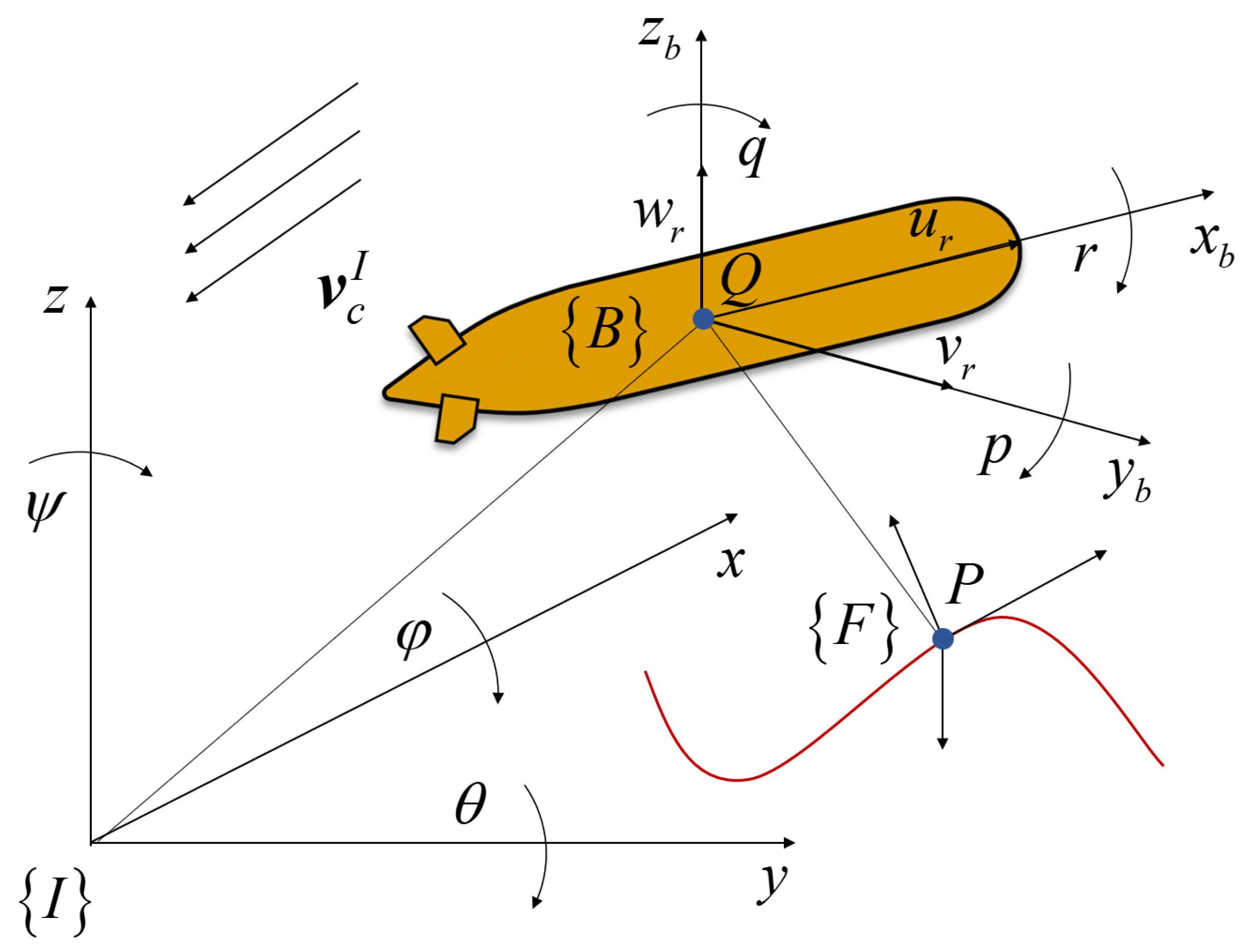
In general, the AUVs work at a certain depth to perform monitoring and sampling missions, etc. Thus, the control problem is always decoupled as a horizontal plane and a vertical plane.

2.1. Notation

The trajectory tracking problem is depicted in Figure 1. $\left\{I\right\}$, $\left\{B\right\}$, and $\left\{F\right\}$ represent the inertial coordinate frame, body-fixed coordinate frame, and Serret–Frenet coordinate frame, respectively. The frame $\left\{I\right\}$ employs the north–east–down (NED) coordinate system. Set the origin of frame $\left\{B\right\}$ coinciding with the center of gravity as Q. Let the referenced trajectory of frame $\left\{F\right\}$ be $P\left(t\right)$ at an arbitrary moment, and the coordinate axes are consistent with the tangent and normal of the referenced trajectory. Set the vehicle pose in frame $\left\{I\right\}$ as $\eta$, and set the referenced trajectory in frame $\left\{I\right\}$ as ${\eta }_d$. Thus, the error pose of the vehicle in frame $\left\{B\right\}$ is set as ${\eta }_e$. Set the flow resultant velocity ${\mathbf{U}}_V={[U,0,0]}^{\top }$ described in frame $\left\{V\right\}$, where $U=\sqrt{u^2+v^2+w^2}$. According to reference [20], the ocean is considered as three-dimensional with non-constant currents, which is always described in frame $\left\{I\right\}$ as ${\mathit{v}}_c^I={[u_c^I,v_c^I,w_c^I]}^T$; that is, ${\dot{\mathit{v}}}_c^I\ne {\ddot{\mathit{v}}}_c^I\ne {\stackrel{⃛}{\mathit{v}}}_c^I\ne \cdots \ne 0$. Therefore, the first-order Gauss–Markov process is introduced to describe the velocities of ocean currents as:

$${\dot{\mathit{v}}}_c^I+{\mu }_c{\mathit{v}}_c^I={\omega }_c$$

(1)

where ${\omega }_c$ is Gaussian white noise and ${\mu }_c\ge 0$ is a constant for the model of time-varying ocean currents [21].

Assumption 1.

The vehicle with a rigid body of uniform mass and neutral buoyancy works in the area of constant salinity [22].

Assumption 2.

The referenced trajectory ${\eta }_d$ is a sufficiently smooth continuous function. Additionally, it is continuously bounded by the first and second time derivatives at least [8].

Remark 1.

The use of the term "pose" implies position ${\mathbf{P}}_d$ and attitude ${\Theta }_d$. As for the vehicle described in frame $\left\{I\right\}$, the surge, sway, and heave are denoted as $\mathbf{P}={[x,y,z]}^T$. The attitude angles of roll, pitch, and yaw are denoted as $\Theta ={[\varphi ,\theta ,\psi ]}^T$.

The models of kinematic and dynamic combining ocean currents are:

$$\begin{array}{cc}\hfill {\mathit{M}}_{RB}\dot{\mathit{v}}& +{\mathit{C}}_{RB}\left(\mathit{v}\right)\mathit{v}+{\mathit{M}}_A{\dot{\mathit{v}}}_r+{\mathit{C}}_A\left({\mathit{v}}_r\right){\mathit{v}}_r+\mathit{D}\left({\mathit{v}}_r\right){\mathit{v}}_r+\mathit{g}\left(\eta \right)=\mathbf{\tau }+\mathit{D}\hfill \\ \hfill \dot{\mathbf{\eta }}=\mathit{J}& \left(\mathbf{\eta }\right){\mathit{v}}_r+{\mathit{v}}_c^I\hfill \end{array}$$

(2)

where the absolute velocity of vehicle in frame $\left\{B\right\}$ is set as $\mathit{v}$, which is measured by DVL, and the current velocity in frame $\left\{B\right\}$ is set as ${\mathit{v}}_c^B$. Therefore, the relative velocity of a vehicle in frame $\left\{B\right\}$ is set as ${\mathit{v}}_r=\mathit{v}-{\mathit{v}}_c^B$. The rotation matrix from frame $\left\{B\right\}$ to frame $\left\{I\right\}$ is defined as $\mathit{J}\left(\eta \right)$; that is, ${\mathit{v}}_c^B=\mathit{J}{\left(\eta \right)}^T{\mathit{v}}_c^I$. In Equation (2), $\mathit{M}$, ${\mathit{C}}_{RB}\left(\mathit{v}\right)$, ${\mathit{C}}_A\left({\mathit{v}}_r\right)$, and $\mathit{D}\left({\mathit{v}}_r\right)$ represent the additional mass matrix, centripetal force matrix, coriolis force matrix, and damping matrix, respectively. $\mathit{g}\left(\eta \right)$, $\mathit{D}$, and $\tau$ are the restorative force (torque) due to buoyancy and gravity, unknown environmental interferences, and control inputs, respectively.

Assumption 3.

All the state variables of vehicle in Equation (2) are measurable [23].

2.2. Model of X-AUV

In this paper, the X-AUV has torpedo-like streamline, maneuverability, rudder efficiency, etc. The following assumptions need to be made.

Assumption 4.

(1) The order of hydrodynamic drag terms in dynamic Equation (2) is less than two. (2) The structure of the X-AUV studied in this paper is symmetrical on three principal axes. (3) The disturbances are decoupled from ocean currents, which ignores the influences of wind and waves, uncertain model parameters, and unknown environmental interferences [10]. The unknown environmental interferences are considered as $\dot{\mathit{D}}=0$ and $\dot{\mathit{D}}\ne 0$.

Assumption 5.

Based on Assumption 4, the parameter perturbation is considered. According to reference [22], the perturbation of hydrodynamic parameters is bounded and does not exceed $20\%$, that is, $|m_{11}-m_{11}^{*}|\le {\overline{m}}_{11}$, $|X_u-X_u^{*}|\le {\overline{X}}_u$, $|X_{\dot{u}}-X_{\dot{u}}^{*}|\le {\overline{X}}_{\dot{u}}$, $|X_{u\left|u\right|}-X_{u\left|u\right|}^{*}|\le {\overline{X}}_{u\left|u\right|}$, $|m_{22}-m_{22}^{*}|\le {\overline{m}}_{22}$, $|Y_v-Y_v^{*}|\le {\overline{Y}}_v$, $|Y_{\dot{v}}-Y_{\dot{v}}^{*}|\le {\overline{Y}}_{\dot{v}}$, $|Y_{v|vs.|}-Y_{v|vs.|}^{*}|\le {\overline{Y}}_{v|vs.|}$, $|m_{33}-m_{33}^{*}|\le {\overline{m}}_{33},\left|Z_w-Z_w^{*}\right|\le {\overline{Z}}_w$, $|Z_{\dot{w}}-Z_{\dot{w}}^{*}|\le {\overline{Z}}_{\dot{w}}$, $|Z_{w\left|w\right|}-Z_{w\left|w\right|}^{*}|\le {\overline{Z}}_{w\left|w\right|}$, $|m_{55}-m_{55}^{*}|\le {\overline{m}}_{55}$, $|M_q-M_q^{*}|\le {\overline{M}}_q$, $|M_{\dot{q}}-M_{\dot{q}}^{*}|\le {\overline{M}}_{\dot{q}}$, $|M_{q\left|q\right|}-M_{q\left|q\right|}^{*}|\le {\overline{M}}_{q\left|q\right|}$, $|m_{66}-m_{66}^{*}|\le {\overline{m}}_{66},\left|N_r-N_r^{*}\right|\le {\overline{N}}_r$, $|N_{\dot{r}}-N_{\dot{r}}^{*}|\le {\overline{N}}_{\dot{r}}$, $|N_{r\left|r\right|}-N_{r\left|r\right|}^{*}|\le {\overline{N}}_{r\left|r\right|}$. ${(·)}^{*}$ represents the nominal values of hydrodynamic parameters, and $\overline{(·)}$ are the upper bounds of hydrodynamic parameters.

Remark 2.

The surge velocity is redefined in the horizontal plane and vertical plane as ${}^{h}u$ and ${}^{v}u$. Beyond that, ${}^h(·)$ represents the symbol in the horizontal plane, and ${}^v(·)$ represents the symbol in the vertical plane.

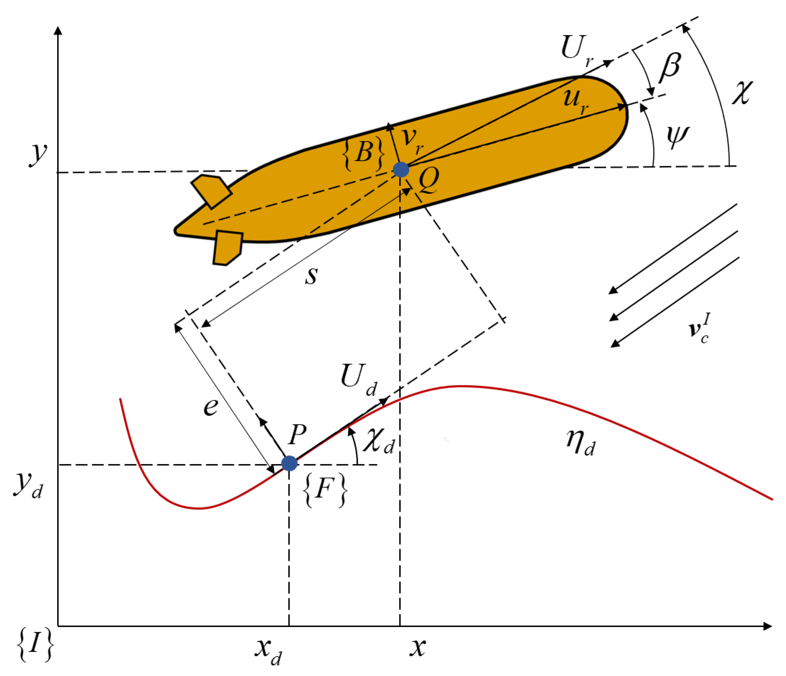
2.2.1. Decoupled Model in the Horizontal Plane

When studying three-DOF motion control in the horizontal plane, the pitch motion is ignored, and according to Equation (2), the kinematics model takes the following form [14]:

$$\begin{array}{cc}\hfill & \dot{x}={}^h{u}_{r}cos\psi -v_{r}sin\psi +u_c^I\hfill \\ \hfill & \dot{y}={}^h{u}_{r}sin\psi +v_{r}cos\psi +v_c^I\hfill \\ \hfill & \dot{\psi }=r\hfill \end{array}$$

(3)

where the absolute velocity of vehicle, the current velocity, and relative velocity of vehicle in frame $\left\{B\right\}$ are decoupled as $\mathit{v}={[{}^{h}u,v,r]}^T$, ${\mathit{v}}_c^B={[u_c,v_c,0]}^T$, and ${\mathit{v}}_r={[{}^h{u}_r,v_r,r]}^T$. The current velocity in frame $\left\{I\right\}$ is decoupled as ${\mathit{v}}_c^I={[u_c^I,v_c^I,0]}^T$; that is, ${\mathit{v}}_c^B={}^h\mathit{J}{\left(\psi \right)}^T{\mathit{v}}_c^I$, where ${}^h\mathit{J}\left(\psi \right)$ is derived as:

$${}^h\mathit{J}\left(\psi \right)=\left[\begin{array}{ccc}cos\psi & -sin\psi & 0\\ sin\psi & cos\psi & 0\\ 0& 0& 1\end{array}\right]$$

(4)

According to Assumption 4, the dynamic model of the X-AUV in the horizontal plane is simplified as follows [18]:

$$\begin{array}{c}\begin{array}{cc}\hfill m_{11}{}^h\dot{u}& =mvr-Y_{\dot{v}}{v}_{r}r-X_u{}^h{u}_r-X_{u\left|u\right|}{}^h{u}_r\left|{}^h{u}_r\right|-X_{\dot{u}}{}^h{\dot{\widehat{u}}}_c^B+{\tau }_u+D_u\hfill \\ \hfill m_{22}\dot{v}& =-mur+X_{\dot{u}}{u}_{r}r-Y_v{v}_r-Y_{v\left|v\right|}{v}_r\left|v_r\right|-Y_{\dot{v}}{\dot{\widehat{v}}}_c^B+D_v\hfill \\ \hfill m_{66}\dot{r}& =\left(Y_{\dot{v}}-X_{\dot{u}}\right)u_r{v}_r-N_{r}r-N_{r\left|r\right|}r\left|r\right|+{\tau }_r+D_r\hfill \end{array}\hfill \end{array}$$

(5)

where m is the mass of vehicle, and the additional mass is expressed as $m_{11}=m-X_{\dot{u}}$, $m_{22}=m-Y_{\dot{v}}$, and $m_{66}=m-N_{\dot{r}}$. The hydrodynamic parameters are expressed as $X_{\left(·\right)}$, $Y_{\left(·\right)}$, and $N_{\left(·\right)}$. The ${}^h{\dot{\widehat{u}}}_c^B$ and ${\dot{\widehat{v}}}_c^B$ represent the time derivatives of estimated currents velocities in frame $\left\{B\right\}$. $D_{\left(·\right)}$ and ${\tau }_{\left(·\right)}$ represent unknown environmental interferences and control inputs.

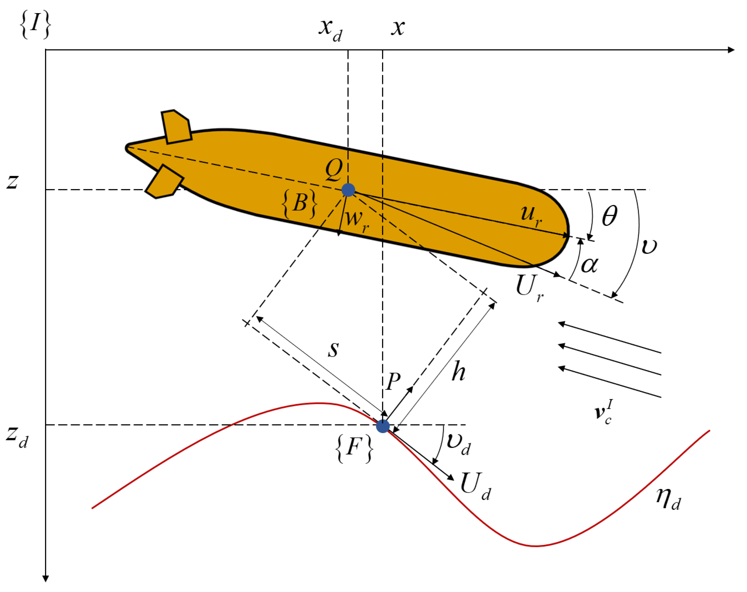
2.2.2. Decoupled Model in the Vertical Plane

Similarly to the idea of horizontal motion, the yaw motion is ignored, and the kinematics model in the vertical plane takes the following form [24]:

$$\begin{array}{c}\dot{x}={}^v{u}_{r}cos\theta +w_{r}sin\theta +u_c^I\hfill \\ \dot{z}=-{}^v{u}_{r}sin\theta +w_{r}cos\theta +w_c^I\hfill \\ \dot{\theta }=q\hfill \end{array}$$

(6)

where each velocity of vehicle is decoupled as $\mathit{v}={[{}^{v}u,w,q]}^T$, ${\mathit{v}}_c^B={[u_c,w_c,0]}^T$, ${\mathit{v}}_r={[{}^h{u}_r,w_r,q]}^T$, and ${\mathit{v}}_c^I={[u_c^I,w_c^I,0]}^T$; that is, ${\mathit{v}}_c^B={}^v\mathit{J}{\left(\theta \right)}^T{\mathit{v}}_c^I$, where ${}^v\mathit{J}\left(\theta \right)$ is derived as follows:

$${}^v\mathit{J}\left(\theta \right)=\left[\begin{array}{ccc}cos\theta & sin\theta & 0\\ -sin\theta & cos\theta & 0\\ 0& 0& 1\end{array}\right]$$

(7)

According to Assumption 4, the dynamic model of X-AUV in the vertical plane is simplified as follows [24]:

$$\begin{array}{c}\begin{array}{cc}\hfill m_{11}{}^v\dot{u}& =-mwq+Z_{\dot{w}}{w}_{r}q-X_u{}^v{u}_r-X_{u\left|u\right|}{}^v{u}_r\left|{}^v{u}_r\right|-X_{\dot{u}}{}^v{\dot{\widehat{u}}}_c^B+{\tau }_u+D_u\hfill \\ \hfill m_{33}\dot{w}& =muq-X_{\dot{u}}{u}_{r}q-Z_w{w}_r-{Z_w}_{\left|w\right|}{w}_r\left|w_r\right|-Z_{\dot{w}}{\dot{\widehat{w}}}_c^B+D_w\hfill \\ \hfill m_{55}\dot{q}& =\left(X_{\dot{u}}-Z_{\dot{w}}\right)u_r{w}_r-M_{q}q-{M_q}_{\left|q\right|}q\left|q\right|+{\tau }_q+D_q\hfill \end{array}\hfill \end{array}$$

(8)

where the additional masses are expressed as $m_{33}=m-Z_{\dot{w}}$ and $m_{55}=m-M_{\dot{q}}$. The hydrodynamic parameters are expressed as $Z_{\left(·\right)}$ and $M_{\left(·\right)}$. The ${}^v{\dot{\widehat{u}}}_c^B$ and ${\dot{\widehat{w}}}_c^B$ represent the time derivatives of the estimated currents’ velocities in frame $\left\{B\right\}$.

Remark 3.

The roll DOF is always neglected by controller in a decoupled subsystem. Due to the inherent metacentric height, assuming $\varphi =p=0$ is not exact in practice [25]. However, the X-AUV is an over-actuated underwater vehicle in attitude space, and the roll DOF is controllable by four ruddders as ${\tau }_p=K_{{\delta }_1}^{*}{u}^2{\delta }_1+K_{{\delta }_2}^{*}{u}^2{\delta }_2+K_{{\delta }_3}^{*}{u}^2{\delta }_3+K_{{\delta }_4}^{*}{u}^2{\delta }_4$, where $K_{(·)}^{*}$ are the nominal parameters of rudder force, and ${\delta }_i$ ($i=1,2,3,4$) are the angle of rudder [26]. The specific PID controller for roll DOF is used according to reference [27].

2.3. Control Objectives

Trajectory tracking control requires a referenced trajectory parameterized by time. It is important to determine the pose errors at an arbitrary time. During the voyage of vehicle, reference [22] ignores the sway velocity v and yaw velocity w, because the surge velocity u is much greater than v and w. Thus, the influences of sideslip angle $\beta$ and attack angle $\alpha$ are no longer considered. However, the assumption in reference [22] only exists at a high velocity and steady motion. In practice, the vehicle is directed by orientation angle in guidance law according to reference [28]. Therefore, this paper considers the orientation angle, which includes azimuth angle $\chi$ and elevation angle $\upsilon$, rather than only considering attitude angle $\Theta$ [10]. Different decoupled planes correspond to different control objectives; thus, the referenced trajectories in frame $\left\{I\right\}$ are defined as follows:

$$\begin{array}{cc}\hfill {}^h{\eta }_d& ={[x_d,y_d,{\chi }_d]}^T\hfill \\ \hfill {}^v{\eta }_d& ={[x_d,z_d,{\upsilon }_d]}^T\hfill \end{array}$$

(9)

where the referenced trajectory is only concerned with path kinematics without path dynamics that help the controller to reduce input and improve efficiency [29]. The desired azimuth angle and desired elevation angle are defined as ${\chi }_d=\arctan ({\dot{y}}_d/{\dot{x}}_d)$ and ${\upsilon }_d=-arctan\left({\dot{z}}_d/\phantom{{\dot{z}}_d{\dot{x}}_d}{\dot{x}}_d\right)$.

Considering the inherent constraints of an X-AUV, the horizontal and vertical curvature of the referenced trajectories are limited as follows:

$$\begin{array}{cc}\hfill {}^h\kappa & =\frac{|{\dot{x}}_d{\ddot{y}}_d-{\ddot{x}}_d{\dot{y}}_d|}{{\left({\dot{x}}_d^2+{\dot{y}}_d^2\right)}^{3/2}}\le \frac{1}{{}^h{\xi }_{min}}\hfill \\ \hfill {}^v\kappa & =\frac{|{\dot{x}}_d{\ddot{z}}_d-{\ddot{x}}_d{\dot{z}}_d|}{{\left({\dot{x}}_d^2+{\dot{z}}_d^2\right)}^{3/2}}\le \frac{1}{{}^v{\xi }_{min}}\hfill \end{array}$$

(10)

where ${}^h{\xi }_{min}$ and ${}^v{\xi }_{min}$ are radii of curvature.

Therefore, the control mission has converted to the poses $\eta \left(t\right)$ that globally converge to the referenced trajectory ${\eta }_{\mathit{d}}\left(t\right)$ within a limited time as follows:

$$\begin{array}{c}\underset{t\to t_h}{lim}\left({}^h\eta \left(t\right)-{}^h{\eta }_d\left(t\right)\right)=0\hfill \\ \underset{t\to t_v}{lim}\left({}^v\eta \left(t\right)-{}^v{\eta }_d\left(t\right)\right)=0\hfill \end{array}$$

(11)

3. Controller Design

In this section, the proposed control scheme consists of the ocean currents observer based on the RESO, a kinematics controller based on the compound LOS guidance law, and a dynamics controller based on the NAITSMC method. The frame of trajectory tracking control is concluded in Figure 2.

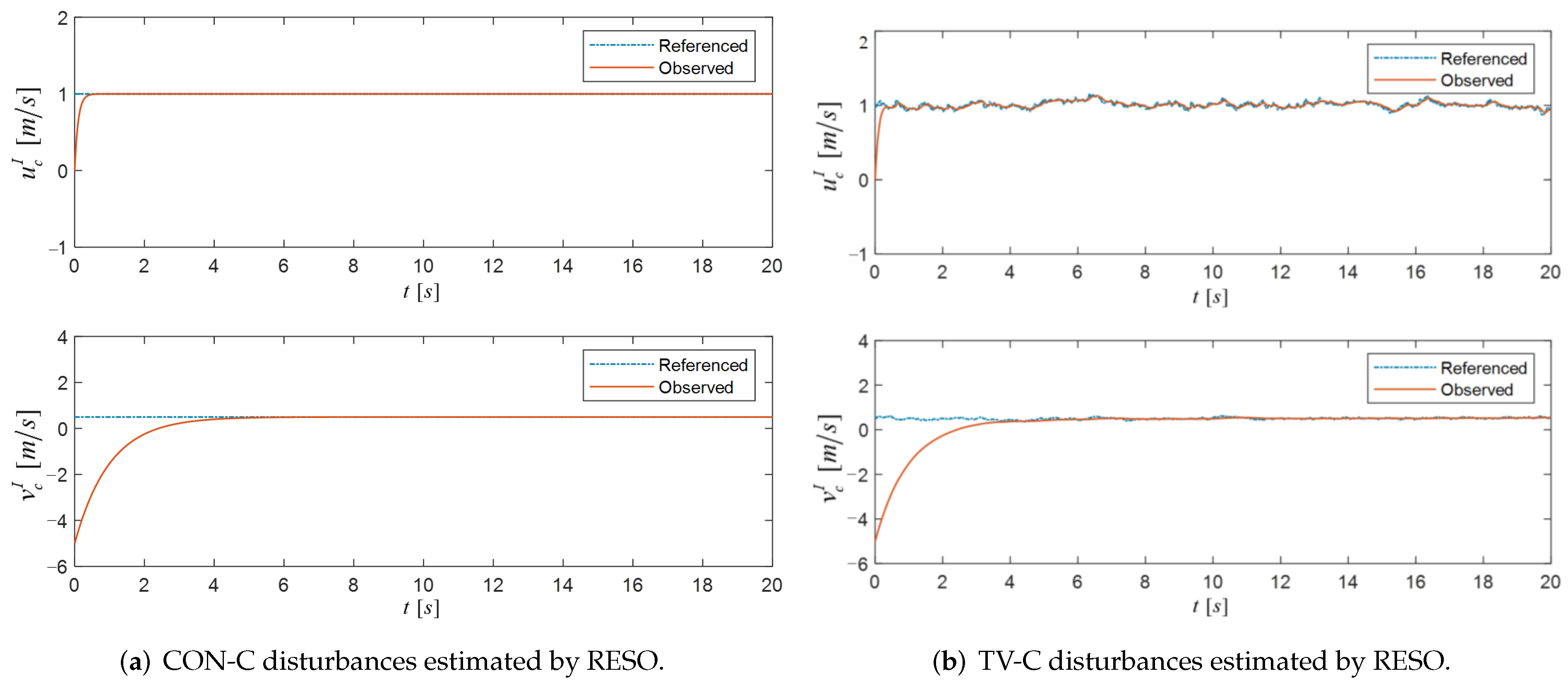
3.1. Ocean Currents Observer

Due to the influence of time-varying, unknown ocean-current disturbances, a RESO is proposed based on reference [30] to estimate the state of ocean currents. The RESOs in different planes are designed as follows:

$$\begin{array}{cc}\hfill {\dot{\delta }}_1& =-{\omega }_1{\delta }_1-{\omega }_1^{2}x-{\omega }_1({}^h{u}_{r}cos\psi -v_{r}sin\psi )\hfill \\ \hfill {}^h{\hat{u}}_c^I& ={\omega }_{1}x+{\delta }_1,{\omega }_1>0\hfill \\ \hfill {\dot{\delta }}_2& =-{\omega }_2{\delta }_1-{\omega }_2^{2}y-{\omega }_2({}^h{u}_{r}sin\psi +v_{r}cos\psi )\hfill \\ \hfill {\hat{v}}_c^I& ={\omega }_{2}y+{\delta }_2,{\omega }_2>0\hfill \end{array}$$

(12)

$$\begin{array}{cc}\hfill {\dot{\delta }}_3& =-{\omega }_3{\delta }_3-{\omega }_3^{2}x-{\omega }_3({}^v{u}_{r}cos\theta +w_{r}sin\theta )\hfill \\ \hfill {}^v{\hat{u}}_c^I& ={\omega }_{3}x+{\delta }_3,{\omega }_3>0\hfill \\ \hfill {\dot{\delta }}_4& =-{\omega }_4{\delta }_4-{\omega }_4^{2}z-{\omega }_4(-{}^v{u}_{r}sin\theta +w_{r}cos\theta )\hfill \\ \hfill {\hat{w}}_c^I& ={\omega }_{4}z+{\delta }_4,{\omega }_4>0\hfill \end{array}$$

(13)

where ${\delta }_i(i=1,2,3,4)$ and ${\omega }_i>0(i=1,2,3,4)$ represent the state of RESO and the gain of observation. The above observers can estimate the velocities of ocean currents as ${}^h{\hat{u}}_c^I$ and ${\hat{v}}_c^I$ in the horizontal plane, and ${}^v{\hat{u}}_c^I$ and ${\hat{w}}_c^I$ in the vertical plane.

3.2. Kinematic Controller Based on Guidance Law

3.2.1. Kinematics Controller in the Horizontal Plane

As shown in Figure 3, according to the control objectives (Equation (11)) in the horizontal plane, set the pose of vehicle and the referenced target as Q and P. The LOS guidance law is designed to track the target based on reference [31]. In the horizontal plane, the rotation matrix ${{}^h\mathbf{R}}_{\mathbf{F}}^{\mathbf{I}}$ from frame $\left\{F\right\}$ to frame $\left\{I\right\}$ is described as:

$${}^h{\mathbf{R}}_{\mathbf{F}}^{\mathbf{I}}=\left[\begin{array}{cc}cos{\chi }_d& -sin{\chi }_d\\ sin{\chi }_d& cos{\chi }_d\end{array}\right]$$

(14)

Based on spatial geometry, the position errors of trajectory tracking are ${}^h{\mathbf{P}}_{\mathbf{e}}={\left[{}^{h}s,e\right]}^{\top }={\left({{}^h\mathbf{R}}_F^I\right)}^{\top }\left(Q-P\right)$, where ${}^{h}s$ and e are represented as along-track error and cross-track error in the horizontal plane [31]. Similarly, the rotation matrix ${{}^h\mathbf{R}}_V^F$ from frame $\left\{V\right\}$ to frame $\left\{F\right\}$ is described as:

$${{}^h\mathbf{R}}_V^F=\left[\begin{array}{cc}cos{\chi }_e& -sin{\chi }_e\\ sin{\chi }_e& cos{\chi }_e\end{array}\right]$$

(15)

where ${\chi }_e$ is the look-ahead angle. The azimuth angle is defined as $\chi =\psi -\beta$, where the sideslip angle is defined as $\beta =arctan\left(v_r/\phantom{v_r{u}_r}{u}_r\right)$[21]. Set the referenced resultant velocity as ${{}^h\mathbf{U}}_d={[{}^h{U}_d,0]}^{\top }$, where ${}^h{U}_d=\sqrt{{\dot{x}}_d^2+{\dot{y}}_d^2}$. The time derivatives of ${}^h{\mathbf{P}}_{\mathbf{e}}$ are calculated as:

$${}^h{\dot{\mathbf{P}}}_{\mathbf{e}}={{}^h\mathbf{S}}_F^{\top }{}^h{\mathbf{P}}_{\mathbf{e}}+{\mathbf{R}}_V^F{\mathbf{U}}_V-{{}^h\mathbf{U}}_d$$

(16)

where the skew-symmetric matrix ${{}^h\mathbf{S}}_F$ is [32]:

$${{}^h\mathbf{S}}_F^{}=\left[\begin{array}{cc}0& -{\dot{\chi }}_d\\ {\dot{\chi }}_d& 0\end{array}\right]$$

(17)

Therefore, Equation (16) is expanded as:

$${}^h{\dot{\mathbf{P}}}_{\mathbf{e}}=\left[\begin{array}{c}-e{\dot{\chi }}_d+Ucos{\chi }_e-{}^h{U}_d\\ {}^{h}s{\dot{\chi }}_d+Usin{\chi }_e\end{array}\right]$$

(18)

According to Equation (11), the control problem of trajectory tracking is converted to the stabilization control of pose errors. Therefore, we selected the following Lyapunov function for position errors as:

$${}^h{V}_{11}=\frac{1}{2}{}^h{s}^2+\frac{1}{2}{e}^2$$

(19)

Take the time derivatives of Equation (19) and simplifying it as:

$${}^h{\dot{V}}_{11}={}^{h}s\left(Ucos{\chi }_e-{}^h{U}_d\right)+eUsin{\chi }_e$$

(20)

Therefore, the LOS guidance law in horizontal plane is designed as:

$${\chi }_e=arctan\left(\frac{-k_{e}e}{{\Delta }_e}\right)$$

(21)

where $k_e>0$ are gain coefficients; the guidance variables ${\Delta }_e>0$. Equation (20) is simplified as:

$${}^h{\dot{V}}_{11}={}^{h}s\left(Ucos{\chi }_e-{}^h{U}_d\right)-\frac{U}{\sqrt{k_e^2{e}^2+{\Delta }_e^2}}{e}^2$$

(22)

After that, the attitude errors are considered with the ${}^h{\dot{V}}_{11}$ Lyapunov function as:

$${}^h{V}_1={}^h{V}_{11}+(1-cos{\chi }_e)$$

(23)

The time derivatives of Equation (23) are calculated as:

$${}^h{\dot{V}}_1={}^{h}s\left(Ucos{\chi }_e-U_d\right)-\frac{U}{\sqrt{k_e^2{e}^2+{\Delta }_e^2}}{e}^2+\left(r+\dot{\beta }-{}^h\kappa {}^h{U}_d\right)sin{\chi }_e$$

(24)

By adopting the idea of virtual velocity, ${}^h{u}_r$ and r are set as virtual control variables. The kinematic controller is designed by referenced virtual velocities to converge ${}^{h}s$ and ${\chi }_e$ to zero within a limited time, that is, $u_d={}^h{u}_r$ and $r_d=r$, to complete trajectory tracking. The virtual velocities were set as follows:

$$\begin{array}{cc}\hfill {}^h{u}_d& =\frac{cos\beta }{cos{\chi }_e}\left({}^h{U}_d+{k_s}^{h}s\right)\hfill \\ \hfill r_d& ={}^h\kappa {}^h{U}_d-\dot{\beta }-k_{r}sin{\chi }_e\hfill \end{array}$$

(25)

where the gains of kinematic controller are $k_s>0$ and $k_r>0$. Let Equation (25) be substituted into Equation (24)—that is, the vehicle is driven by ${}^h{u}_d$ and $r_d$; ${\dot{V}}_1$ is expressed as:

$${}^h{\dot{V}}_1=-k_s{}^h{s}^2-\frac{U}{\sqrt{k_e^2{e}^2+{\Delta }_e^2}}{e}^2-k_r{sin}^2{\chi }_e$$

(26)

By designing parameters $k_s$, $k_e$, and $k_r$, ${}^h{\dot{V}}_1\le 0$ is guaranteed, if and only if ${}^{h}s$, e, and ${\chi }_e$ are zero; ${}^h{\dot{V}}_1=0$. Thus, ${}^h{\dot{V}}_1$ is negative semi-definite.

3.2.2. Kinematics Controller in the Vertical Plane

As shown in Figure 4 in the vertical plane, the rotation matrix ${{}^v\mathbf{R}}_{\mathbf{F}}^{\mathbf{I}}$ from frame $\left\{F\right\}$ to frame $\left\{I\right\}$ is described as:

$${}^v{\mathbf{R}}_{\mathbf{F}}^{\mathbf{I}}=\left[\begin{array}{cc}cos{\upsilon }_d& sin{\upsilon }_d\\ -sin{\upsilon }_d& cos{\upsilon }_d\end{array}\right]$$

(27)

The position errors of trajectory tracking are ${}^v{\mathbf{P}}_{\mathbf{e}}={\left[{}^{v}s,h\right]}^{\top }={\left({{}^v\mathbf{R}}_F^I\right)}^{\top }\left(Q-P\right)$, where ${}^{v}s$ and h represent along-track error and vertical-track error [31]. Similarly, the rotation matrix ${{}^v\mathbf{R}}_V^F$ from frame $\left\{V\right\}$ to frame $\left\{F\right\}$ is described as:

$${{}^v\mathbf{R}}_V^F=\left[\begin{array}{cc}cos{\upsilon }_e& sin{\upsilon }_e\\ -sin{\upsilon }_e& cos{\upsilon }_e\end{array}\right]$$

(28)

where ${\upsilon }_e$ is the look-ahead angle. The elevation angle is defined as $\upsilon =\theta -\alpha$, where the attack angle is defined as $\alpha =arctan\left(w_r/\phantom{w_r{u}_r}{u}_r\right)$[21]. Set the referenced resultant velocity as ${{}^v\mathbf{U}}_d={[{}^v{U}_d,0]}^{\top }$, where ${}^v{U}_d=\sqrt{{\dot{x}}_d^2+{\dot{z}}_d^2}$. The time derivatives of ${}^v{\mathbf{P}}_{\mathbf{e}}$ are calculated as:

$${}^v{\dot{\mathbf{P}}}_{\mathbf{e}}={{}^v\mathbf{S}}_F^{\top }{}^v{\mathbf{P}}_{\mathbf{e}}+{{}^v\mathbf{R}}_V^F{\mathbf{U}}_V-{{}^v\mathbf{U}}_d$$

(29)

where the skew-symmetric matrix ${{}^v\mathbf{S}}_F$ is [32]:

$${{}^v\mathbf{S}}_F^{}=\left[\begin{array}{cc}0& {\dot{\upsilon }}_d\\ -{\dot{\upsilon }}_d& 0\end{array}\right]$$

(30)

Therefore, Equation (29) is expanded as:

$${}^v{\dot{\mathbf{P}}}_{\mathbf{e}}=\left[\begin{array}{c}h{\dot{v}}_d+Ucos{v}_e-{}^v{U}_d\\ -s{\dot{v}}_d-Usin{v}_e\end{array}\right]$$

(31)

Similarly to the inference of horizontal plane, the following Lyapunov function for pose errors is:

$${}^v{V}_2=\frac{1}{2}{}^v{s}^2+\frac{1}{2}{h}^2+(1-cos{\upsilon }_e)$$

(32)

The kinematics control law and guidance law in the vertical plane are given directly as:

$$\begin{array}{cc}\hfill {}^v{u}_d& =\frac{cos\alpha }{cos{v}_e}\left({}^v{U}_d+k_s{}^{v}s\right)\hfill \\ \hfill v_e& =arctan\left(\frac{k_{h}h}{{\Delta }_h}\right)\hfill \\ \hfill q_d& ={}^v\kappa {}^v{U}_d+\dot{\alpha }-k_{q}sin{\upsilon }_e\hfill \end{array}$$

(33)

where $k_s>0$, $k_h>0$, and $k_q>0$; the guidance variables ${\Delta }_h>0$. The time derivatives of Equation (32) are simplified as:

$${}^v{\dot{V}}_2=-k_s{}^v{s}^2-\frac{U}{\sqrt{k_h^2{h}^2+{\Delta }_h^2}}{h}^2-k_q{sin}^2{\upsilon }_e$$

(34)

By designing the parameters $k_s$, $k_h$, and $k_q$, ${}^v{\dot{V}}_2\le 0$ is guaranteed, if and only if ${}^{v}s$, h, and ${\upsilon }_e$ are zero; ${}^v{\dot{V}}_2=0$. Thus, ${}^v{\dot{V}}_2$ is negative semi-definite, and the trajectory tracking errors can be stabilized.

3.3. Dynamic Controller

3.3.1. Dynamic Controller in the Horizontal Plane

The velocity is not a controllable variable; therefore, the dynamic controller is designed to converge on the referenced virtual velocity based on the kinematics controller. Define the virtual velocities errors of trajectory tracking in the horizontal plane as follows:

$$\begin{array}{cc}\hfill {}^h{u}_e& =u_r-{}^h{u}_d\hfill \\ \hfill r_e& =r-r_d\hfill \end{array}$$

(35)

By substituting Equation (5) into the time derivatives of Equation (35), and also considering time-varying unknown ocean-current disturbances, the differential equations for the errors of velocities are obtained as follows:

$$\begin{array}{cc}\hfill {}^h{\dot{u}}_e& =\frac{1}{m_{11}}(mvr-Y_{\dot{v}}{v}_{r}r-X_u{}^h{u}_r-X_{u\left|u\right|}{}^h{u}_r|{}^h{u}_r|+{\tau }_u+D_u-m^h{\dot{\hat{u}}}_c^B-m_{11}{}^h{\dot{u}}_d)\hfill \\ \hfill {\dot{r}}_e& =\frac{1}{m_{66}}(\left(Y_{\dot{v}}-X_{\dot{u}}\right)u_r{v}_r-N_{r}r-N_{r\left|r\right|}r|r|+{\tau }_r+D_r-m_{66}{\dot{r}}_d)\hfill \end{array}$$

(36)

To date, the trajectory tracking problem has been converted into designing the dynamic controller of ${}^h{\tau }_u$ and ${\tau }_r$ to stabilize the errors of velocities ${}^h{u}_e$ and $r_e$[33]. Therefore, the NAITSMC is proposed, and the sliding mode surface related to ${}^h{u}_e$ is chosen as:

$${}^h{S}_u=\frac{q_u}{p_u}{\beta }_u{\lambda }_u{\int }_0^1{}^h{u}_e\left(\tau \right)d\tau +{\beta }_u{}^h{u_e}^{q_u/\phantom{q_u{p}_u}{p}_u}$$

(37)

where ${\lambda }_u>0$ and ${\beta }_u>0$ are constants, and the positive odd integers $q_u$ and $p_u$ satisfy $1<q_u/\phantom{1<q_u{p}_u}{p}_u<2$. Substitute Equation (36) into the time derivatives of Equation (37) as follows:

$${}^h{\dot{S}}_u=\frac{q_u{\beta }_u{}^h{u_e}^{\left(q_u/\phantom{q_u{p}_u}{p}_u-1\right)}}{p_u{m}_{11}}(mvr-Y_{\dot{v}}{v}_{r}r-X_u{}^h{u}_r-X_{u\left|u\right|}{}^h{u}_r|{}^h{u}_r|+{\tau }_u+D_u-m^h{\dot{\hat{u}}}_c^B-m_{11}{}^h{\dot{u}}_d+m_{11}{\lambda }_u{}^h{u_e}^{\left(2-q_u/\phantom{q_u{p}_u}{p}_u\right)})$$

(38)

In order to let $u_e$ converge to zero along with sliding mode surface $S_u$ from an arbitrary initial position, the equivalent control law ${\tau }_u^{eq}$ is designed as follows:

$${}^h{\tau }_u^{eq}=-mvr+Y_{\dot{v}}^{*}{v}_{r}r+X_u^{*}{}^h{u}_r+X_{u\left|u\right|}^{*}{}^h{u}_r\left|{}^h{u}_r\right|-{}^h{\hat{D}}_u+m^h{\dot{\hat{u}}}_c^B+m_{11}^{*}{}^h{\dot{u}}_d-m_{11}^{*}{\lambda }_u{}^h{u_e}^{\left(2-q_u/\phantom{q_u{p}_u}{p}_u\right)}$$

(39)

where the nominal values of hydrodynamic parameters are used in Equation (39) for the X-AUV. Define the estimation of unknown environmental interference as ${}^h{\hat{D}}_u$, and it will be introduced in the following page. The switching control law ${\tau }_u^{sw}$ is designed as follows:

$${}^h{\tau }_u^{sw}=-{\xi }_{u}sign\left({}^h{S}_u\right)$$

(40)

where ${\xi }_u$ is the coefficient of the sliding-mode reaching law to be designed about the upper bound of the parameter perturbation.

Considering the chattering problem in practical control, the concept of a boundary layer is utilized to replace the $sign\left(\right)$ function in the control law with the nonlinear saturation function $sat\left(S\right)$ as follows:

$$sat\left(S\right)=\left\{\begin{array}{cc}\hfill -1,& S<-\rho \hfill \\ \hfill \frac{S}{\rho },& -\rho \le S\le \rho \hfill \\ \hfill 1,& \rho <S\hfill \end{array}\right.$$

(41)

where $\rho$ denotes the limit of saturation.

Combining Equations (39) and (40), the dynamic control law of surge ${}^h{\tau }_u$ is designed as follows:

$${}^h{\tau }_u=-mvr+Y_{\dot{v}}^{*}{v}_{r}r+X_u^{*}{}^h{u}_r+X_{u\left|u\right|}^{*}{}^h{u}_r\left|{}^h{u}_r\right|+m_{11}^{*}{}^h{\dot{u}}_d-m_{11}^{*}{\lambda }_u{}^h{u_e}^{\left(2-q_u/\phantom{q_u{p}_u}{p}_u\right)}+m^h{\dot{\hat{u}}}_c^B-{}^h{\hat{D}}_u-{}^h{\xi }_{u}sat\left({}^h{S}_u\right)$$

(42)

Considering the stability of ${}^h{S}_u$ and ${}^h{\hat{D}}_u$ under unknown disturbance, the following candidate Lyapunov function is set as:

$${}^h{V}_{2u}=\frac{1}{2}{m}_{11}{}^h{S}_u^2+\frac{1}{2}{\mu }_u{}^h{\tilde{D}}_u^2$$

(43)

where ${\mu }_u>0$; the errors in the estimation of unknown environmental interferences are defined as ${}^h{\tilde{D}}_u=D_u-{}^h{\hat{D}}_u$; and the time derivatives of Equation (43) are:

$$\begin{array}{cc}\hfill & {}^h{\dot{V}}_{2u}=m_{11}{}^h{S}_u{}^h{\dot{S}}_u+{\mu }_u{}^h{\tilde{D}}_u({\dot{D}}_u-{}^h{\dot{\hat{D}}}_u)\hfill \\ \hfill & ={}^h{S}_u\frac{q_u{\beta }_u{}^h{u_e}^{\left(q_u/\phantom{q_u{p}_u}{p}_u-1\right)}}{p_u}((Y_{\dot{v}}^{*}-Y_{\dot{v}})v_{r}r+(X_u^{\ast }-X_u){}^h{u}_r+(X_{u\left|u\right|}^{\ast }-X_{u\left|u\right|}){}^h{u}_r\left|{}^h{u}_r\right|\hfill \\ \hfill & +(m_{11}^{\ast }-m_{11}){}^h{\dot{u}}_d-(m_{11}^{\ast }-m_{11}){\lambda }_u{}^h{u_e}^{\left(2-q_u/\phantom{q_u{p}_u}{p}_u\right)}+{}^h{\tilde{D}}_u-{}^h{\xi }_{u}sat\left({}^h{S}_u\right))+{\mu }_u{}^h{\tilde{D}}_u\left({\dot{D}}_u-{}^h{\dot{\hat{D}}}_u\right)\hfill \\ \hfill & \le {\beta }_u{\xi }_u\left|{}^h{S}_u\right|+{\mu }_u{}^h{\tilde{D}}_u{\dot{D}}_u+{\mu }_u{}^h{\tilde{D}}_u\left({\mu }_u^{-1}{}^h{S}_u{\beta }_u-{}^h{\dot{\hat{D}}}_u\right)\hfill \end{array}$$

(44)

According to Assumption 5, the coefficient of the sliding-mode reaching law ${\xi }_u$ is designed as follows:

$${}^h{\xi }_u={\overline{Y}}_{\dot{v}}|v_{r}r|+{\overline{X}}_u|{}^h{u}_r|+{\overline{X}}_{u\left|u\right|}{}^h{u}_r^2+{\overline{m}}_{11}|{}^h{\dot{u}}_d|+{\overline{m}}_{11}{\lambda }_u\left|{}^h{u_e}^{\left(2-q_u/\phantom{q_u{p}_u}{p}_u\right)}\right|+{\zeta }_u$$

(45)

where ${\zeta }_u>0$. Substitute Equation (45) into Equation (44), as for $1<q_u/\phantom{1<q_u{p}_u}{p}_u<2$; that is, $u_e^{\left(q_u/\phantom{q_u{p}_u}{p}_u-1\right)}\le |u_e{|}^{\left(q_u/\phantom{q_u{p}_u}{p}_u-1\right)}$, and it is simplified as follows:

$${}^h{\dot{V}}_{2u}\le -{\beta }_u{\zeta }_u\left|{}^h{S}_u\right|+{\mu }_u{}^h{\tilde{D}}_u{\dot{D}}_u+{\mu }_u{}^h{\tilde{D}}_u\left({\mu }_u^{-1}{}^h{S}_u{\beta }_u-{}^h{\dot{\hat{D}}}_u\right)$$

(46)

Therefore, the adaptive interference law is designed by Equation (46) as follows:

$${}^h{\dot{\hat{D}}}_u={\mu }_u^{-1}{}^h{S}_u{\beta }_u$$

(47)

After substituting Equation (47) into Equation (46), ${}^h{\dot{V}}_{2u}$ is:

$${}^h{\dot{V}}_{2u}\le -{\beta }_u{\xi }_u\left|{}^h{S}_u\right|+{\mu }_u{}^h{\tilde{D}}_u{\dot{D}}_u$$

(48)

Remark 4.

Due to $1<q_u/\phantom{1<q_u{p}_u}{p}_u<2$, so that $0<q_u/\phantom{1<q_u{p}_u}{p}_u-1<1$ and $0<2-q_u/\phantom{1<q_u{p}_u}{p}_u<1$ in Equations (29) and (35). Therefore, the errors of velocity ${\mathit{v}}^{q_u/\phantom{q_u{p}_u}{p}_u-1}$ and ${\mathit{v}}^{2-q_u/\phantom{2-q_u{p}_u}{p}_u}(\mathit{v}=[u_e,q_e,r_e])$ will not diverge; thus, the proposed method is non-singular [34].

In the horizontal plane, the dynamic control law of yaw ${\tau }_r$ is similar to the dynamic control law of surge ${}^h{\tau }_u$; therefore, the main results of the relevant control law are given directly. The sliding mode surfaces related to $r_e$ were chosen as follows:

$$S_r=\frac{q_r}{p_r}{\beta }_r{\lambda }_r{\int }_0^1{r}_e\left(\tau \right)d\tau +{\beta }_r{r_e}^{q_r/\phantom{q_r{p}_r}{p}_r}$$

(49)

Substitute Equation (36) into the time derivatives of Equation (49) as follows:

$${\dot{S}}_r=\frac{q_r{\beta }_r{u_r}^{\left(q_r/\phantom{q_r{p}_r-1}{p}_r-1\right)}}{p_r{m}_{66}}(\left(Y_{\dot{v}}-X_{\dot{u}}\right)u_r{v}_r-N_{r}r-N_{r\left|r\right|}r|r|+{\tau }_r+D_r-m_{66}{\dot{r}}_d+m_{66}{\lambda }_r{r_e}^{\left(2-{q_r/\phantom{q_{r}p}p}_r\right)})$$

(50)

The dynamic control law of yaw ${\tau }_r$ is designed as follows:

$${\tau }_r=-\left(Y_{\dot{v}}^{\ast }-X_{\dot{u}}^{\ast }\right)u_r{v}_r+N_r^{\ast }r+N_{r\left|r\right|}^{\ast }r\left|r\right|+m_{66}^{\ast }{\dot{r}}_d-m_{66}^{\ast }{\lambda }_r{r_e}^{\left(2-{q_r/\phantom{q_{r}p}p}_r\right)}-{\hat{D}}_r-{\xi }_{r}sat\left(S_r\right)$$

(51)

where the coefficient of the sliding-mode reaching law ${\xi }_r$ is designed based on Assumption 5 as follows:

$${\xi }_r=\left({\overline{Y}}_{\dot{v}}^{}-{\overline{X}}_{\dot{u}}^{}\right)|u_r{v}_r|+{\overline{N}}_r^{}\left|r\right|+N_{r\left|r\right|}^{\ast }{r}^2+{\overline{m}}_{66}|{\dot{r}}_d|+{\overline{m}}_{66}{\lambda }_r\left|{r_e}^{\left(2-{q_r/\phantom{q_{r}p}p}_r\right)}\right|+{\zeta }_r$$

(52)

Therefore, the time derivatives of candidate Lyapunov functions and ${\dot{V}}_{2r}$ are simplified as follows:

$${\dot{V}}_{2r}\le -{\beta }_r{\zeta }_r\left|S_r\right|+{\mu }_r{\tilde{D}}_r{\dot{D}}_r+{\mu }_r{\tilde{D}}_r\left({\mu }_r^{-1}{S}_r{\beta }_r-{\dot{\hat{D}}}_r\right)$$

(53)

The adaptive interference law ${\hat{D}}_r$ is designed by Equation (53) as follows:

$${\dot{\hat{D}}}_r={\mu }_r^{-1}{S}_r{\beta }_r$$

(54)

where ${\mu }_r>0$.

3.3.2. Dynamic Controller in the Vertical Plane

Similarly to the inference of the horizontal plane, the main processes of the dynamic controller in the vertical plane are given directly as follows. The errors of virtual velocities are:

$$\begin{array}{cc}\hfill {}^v{u}_e& =u_r-{}^v{u}_d\hfill \\ \hfill q_e& =q-q_d\hfill \end{array}$$

(55)

Substitute Equation (8) into the time derivatives of Equation (55) as:

$$\begin{array}{cc}\hfill {}^v{\dot{u}}_e& =\frac{1}{m_{11}}(-mwq+Z_{\dot{w}}{w}_{r}q-X_u{}^v{u}_r-X_{u\left|u\right|}{}^v{u}_r|{}^v{u}_r|+{\tau }_u+D_u-m{}^v{\dot{\hat{u}}}_c^B-m_{11}{}^v{\dot{u}}_d)\hfill \\ \hfill {\dot{q}}_e& =\frac{1}{m_{55}}(\left(X_{\dot{u}}-Z_{\dot{w}}\right)u_r{w}_r-M_{q}q-{M_q}_{\left|q\right|}q|q|+{\tau }_q+D_q-m_{55}{\dot{q}}_d)\hfill \end{array}$$

(56)

The sliding mode surfaces ${}^v{S}_u$ and $S_q$ related to the errors of velocities ${}^v{u}_e$ and $q_e$ were chosen as follows:

$$\begin{array}{cc}\hfill {}^v{S}_u& =\frac{q_u}{p_u}{\beta }_u{\lambda }_u{\int }_0^1{}^v{u}_e\left(\tau \right)d\tau +{\beta }_u{}^v{u_e}^{q_u/\phantom{q_u{p}_u}{p}_u}\hfill \\ \hfill S_q& =\frac{q_q}{p_q}{\beta }_q{\lambda }_q{\int }_0^1{q}_e\left(\tau \right)d\tau +{\beta }_q{q_e}^{q_q/\phantom{q_q{p}_q}{p}_q}\hfill \end{array}$$

(57)

Substitute Equation (56) into the time derivatives of Equation (57) as follows:

$$\begin{array}{cc}\hfill {}^v{\dot{S}}_u& =\frac{q_u{\beta }_u{}^v{u_e}^{\left(q_u/\phantom{q_u{p}_u-1}{p}_u-1\right)}}{p_u{m}_{11}}(-mwq+Z_{\dot{w}}{w}_{r}q-X_u{}^v{u}_r-X_{u\left|u\right|}{}^v{u}_r\left|{}^v{u}_r\right|+{\tau }_u+D_u\hfill \\ \hfill & -m{}^v{\dot{\hat{u}}}_c^B-m_{11}{}^v{\dot{u}}_d+m_{11}{\lambda }_u{}^v{u_e}^{\left(2-q_u/\phantom{q_u{p}_u}{p}_u\right)})\hfill \\ \hfill {\dot{S}}_q& =\frac{q_q{\beta }_q{q_e}^{\left(q_q/\phantom{q_q{p}_q-1}{p}_q-1\right)}}{p_q{m}_{55}}(\left(X_{\dot{u}}-Z_{\dot{w}}\right)u_r{w}_r-M_{q}q-{M_q}_{\left|q\right|}q\left|q\right|+{\tau }_q+D_q\hfill \\ \hfill & -m_{55}{\dot{q}}_d+m_{55}{\lambda }_q{q_e}^{\left(2-q_q/\phantom{q_q{p}_q}{p}_q\right)})\hfill \end{array}$$

(58)

The dynamic control laws of surge ${}^v{\tau }_u$ and ${\tau }_q$ pitch are designed as follows:

$$\begin{array}{cc}\hfill {}^v{\tau }_u& =mwq-Z_{\dot{w}}^{\ast }{w}_{r}q+X_u^{\ast }{}^v{u}_r+X_{u\left|u\right|}^{\ast }{}^v{u}_r\left|{}^v{u}_r\right|+m_{11}^{\ast }{}^v{\dot{u}}_d-m_{11}^{\ast }{\lambda }_u{}^v{u_e}^{\left(2-q_u/\phantom{q_u{p}_u}{p}_u\right)}+m{}^v{\dot{\hat{u}}}_c^B-{}^v{\hat{D}}_u-{}^v{\xi }_{u}sat\left({}^v{S}_u\right)\hfill \\ \hfill {\tau }_q& =-\left(X_{\dot{u}}^{\ast }-Z_{\dot{w}}^{\ast }\right)u_r{w}_r+M_q^{\ast }q+M_{q\left|q\right|}^{\ast }q\left|q\right|+m_{55}^{\ast }{\dot{q}}_d-m_{55}^{\ast }{\lambda }_q{r_e}^{\left(2-{q_q/\phantom{q_{q}p}p}_q\right)}-{\hat{D}}_q-{\xi }_{q}sat\left(S_q\right)\hfill \end{array}$$

(59)

The coefficients of sliding-mode reaching laws ${}^v{\xi }_u$ and ${\xi }_q$ are designed based on Assumption 5 as follows:

$$\begin{array}{cc}\hfill {}^v{\xi }_u& ={\overline{Z}}_{\dot{w}}^{}|w_{r}q|+{\overline{X}}_u|{}^v{u}_r|+{\overline{X}}_{u\left|u\right|}{}^v{u}_r^2+{\overline{m}}_{11}|{}^v{\dot{u}}_d|+{\overline{m}}_{11}{\lambda }_u\left|{}^v{u_e}^{\left(2-q_u/\phantom{q_u{p}_u}{p}_u\right)}\right|+{\zeta }_u\hfill \\ \hfill {\xi }_q& =\left({\overline{Z}}_{\dot{w}}^{}-{\overline{X}}_{\dot{u}}^{}\right)|u_r{w}_r|+{\overline{M}}_q^{}\left|q\right|+{\overline{M}}_{q\left|q\right|}^{}{q}^2+{\overline{m}}_{55}|{\dot{q}}_d|+{\overline{m}}_{55}{\lambda }_q\left|{r_e}^{\left(2-{q_q/\phantom{q_{q}p}p}_q\right)}\right|+{\zeta }_q\hfill \end{array}$$

(60)

The adaptive interference laws ${}^v{\hat{D}}_u$ and ${\hat{D}}_q$ are designed as follows:

$$\begin{array}{cc}\hfill {}^v{\dot{\hat{D}}}_u& ={\mu }_u^{-1}{}^v{S}_u{\beta }_u\hfill \\ \hfill {\dot{\hat{D}}}_q& ={\mu }_q^{-1}{S}_q{\beta }_q\hfill \end{array}$$

(61)

where ${\mu }_u>0$ and ${\mu }_q>0$.

4. Stability Analysis

Proposition 1.

Focused on the horizontal plane, the X-AUV, based on the kinematics and dynamic model Equation (2), utilizes the kinematics tracking error model, Equation (18), to track a referenced trajectory satisfying Assumption 2, under the kinematics control law of virtual velocity, Equation (25), based on the compound orientation angle, the dynamic control law of NAITSMC, Equations (42) and (51), and the adaptive interference law, Equations (47) and (54); the pose errors, Equation (9), and virtual velocity errors, Equation (35), are guaranteed global asymptotic stability for the overall control system, and are non-singular form Remark 4.

Proof of Proposition 1.

For the overall control system in the horizontal plane, the following candidate Lyapunov function is defined as:

$${}^h{V}_3={}^h{V}_1+{}^h{V}_{2u}+V_{2r}$$

(62)

Differentiating Equation (62) and substituting Equations (26), (48), and (53) yields:

$${}^h{\dot{V}}_3\le -k_s{}^h{s}^2-\frac{U}{\sqrt{k_e^2{e}^2+{\Delta }_e^2}}{e}^2-k_r{sin}^2{\chi }_e-{\beta }_u{\zeta }_u\left|{}^h{S}_u\right|-{\beta }_r{\zeta }_r\left|S_r\right|+{\mu }_u{}^h{\tilde{D}}_u{\dot{D}}_u+{\mu }_r{\tilde{D}}_r{\dot{D}}_r$$

(63)

According to Assumption 4, the time derivatives of unknown environmental interferences ${\dot{D}}_u$ and ${\dot{D}}_r$ have three conditions. Let us take ${\dot{D}}_u$ as an example as follows:

• If ${\dot{D}}_u=0$, ${\mu }_u{}^h{\tilde{D}}_u{\dot{D}}_u=0$.
• If ${\dot{D}}_u>0$, ${}^h{\tilde{D}}_u=D_u-{}^h{\hat{D}}_u<0$, then ${\mu }_u{}^h{\tilde{D}}_u{\dot{D}}_u<0$.
• If ${\dot{D}}_u<0$, ${}^h{\tilde{D}}_u=D_u-{}^h{\hat{D}}_u>0$, then ${\mu }_u{}^h{\tilde{D}}_u{\dot{D}}_u<0$.

Therefore, whatever ${\dot{D}}_u$ state, ${\mu }_u{}^h{\tilde{D}}_u{\dot{D}}_u\le 0$. Similarly, ${\mu }_r{\tilde{D}}_r{\dot{D}}_r\le 0$.

For the overall control system in the horizontal plane, if $D_u$ and $D_r$ are slow time-varying, Equation (63) is simplified as:

$${}^h{\dot{V}}_3\le -k_s{}^h{s}^2-\frac{U}{\sqrt{k_e^2{e}^2+{\Delta }_e^2}}{e}^2-k_r{sin}^2{\chi }_e-{\beta }_u{\zeta }_u\left|{}^h{S}_u\right|-{\beta }_r{\zeta }_r\left|S_r\right|\le 0$$

(64)

If and only if ${}^{h}s=0$, $e=0$, ${\chi }_e=0$, ${}^h{u}_e=0$, and $r_e=0$, so that ${}^h{\dot{V}}_3=0$. According to LaSalle’s invariance principle, the system asymptotically converges to zero according to Lyapunov’s second stability theorem.

For Equation (63), if $D_u$ and $D_r$ are not slowly time-varying, the system also satisfies the Lyapunov stability theorem that the tracking errors converge to a bounded range by changing the controller parameters.

By the above processes, Proposition 1 can be proofed. □

5. Numerical Simulations

The numerical simulations were divided into three parts to verify the proposed controller under unknown time-varying disturbances in the horizontal plane and vertical plane. Thus, three missions were performed with three control methods: (1) Method 1, SMC control. (2) Method 2, PID control. (3) Proposed method. The above methods were influenced by non-currents (NON-C); constant currents (CON-C), which were set as $[u_c,v_c]=[1,0.5]$; and time-varying currents (TV-C). The simulation cases are summarized in

Table 1. The simulation cases.

NO.	Methods	Plane	Environment	Purpose
Case I	Above methods	Horizontal Plane	CON-C disturbances	Verify the validity of NAITSMC method
Case II	Proposed	Horizontal Plane	CON-C, TV-C, and NON-C disturbances	Verify the robustness of NAITSMC method
Case III	Above methods	Vertical Plane	TV-C disturbances	Verify the vertical performance of NAITSMC method

.

The main parameters of proposed scheme were set as: ${\omega }_1=10,{\omega }_2=1,{\omega }_3=10,{\omega }_4=1$ (for the RESO), $k_s=0.5,k_r=5,k_e=1$ (for the kinematics controller in the horizontal plane), $k_s=0.5,k_q=5,k_h=1$ (for the kinematics controller in the vertical plane), and $q_i/\phantom{q_i{p}_i}{p}_i=1.4,{\beta }_i=0.5,{\lambda }_i=5,{\zeta }_i=2,{\mu }_i=10$, where $i=u,q,r$ (for the dynamic controller). The hydrodynamic parameters of X-AUV are summarized in

Table 2. The hydrodynamic parameters of X-AUV [35].

$X_u=0\mathrm{kg}/\mathrm{s}$	$Z_{w\left|w\right|}=-141.69\mathrm{kg}/\mathrm{m}$
$X_{\dot{u}}=-2.52\mathrm{kg}$	$M_q=-23.76\mathrm{kg}·{\mathrm{m}}^2/(\mathrm{s}·\mathrm{rad})$
$X_{u\left|u\right|}=-6.45\mathrm{kg}/\mathrm{m}$	$M_{\dot{q}}=-5.43\mathrm{kg}·{\mathrm{m}}^2$
$Y_v=-49.12\mathrm{kg}/\mathrm{s}$	$M_{q\left|q\right|}=-3.89\mathrm{kg}/\mathrm{m}$
$Y_{\dot{v}}=-4.91\mathrm{kg}$	$N_r=-27.20\mathrm{kg}·{\mathrm{m}}^2/(\mathrm{s}·\mathrm{rad})$
$Y_{v\left|v\right|}=-182.22\mathrm{kg}/\mathrm{m}$	$N_{\dot{r}}=-5.44\mathrm{kg}·{\mathrm{m}}^2$
$Z_w=-46.67\mathrm{kg}/\mathrm{s}$	$N_{r\left|r\right|}=-4.91\mathrm{kg}/\mathrm{m}$
$Z_{\dot{w}}=-4.91\mathrm{kg}$	$m=45\mathrm{kg}$

. Additionally, the parameters were added with 20% perturbations to verify the robustness and adaptability of NAITSMC method. All simulations were run on an AMD Ryzen 7 5800H with a Radeon Graphics 3.20 GHz PC with 16 GB of memory.

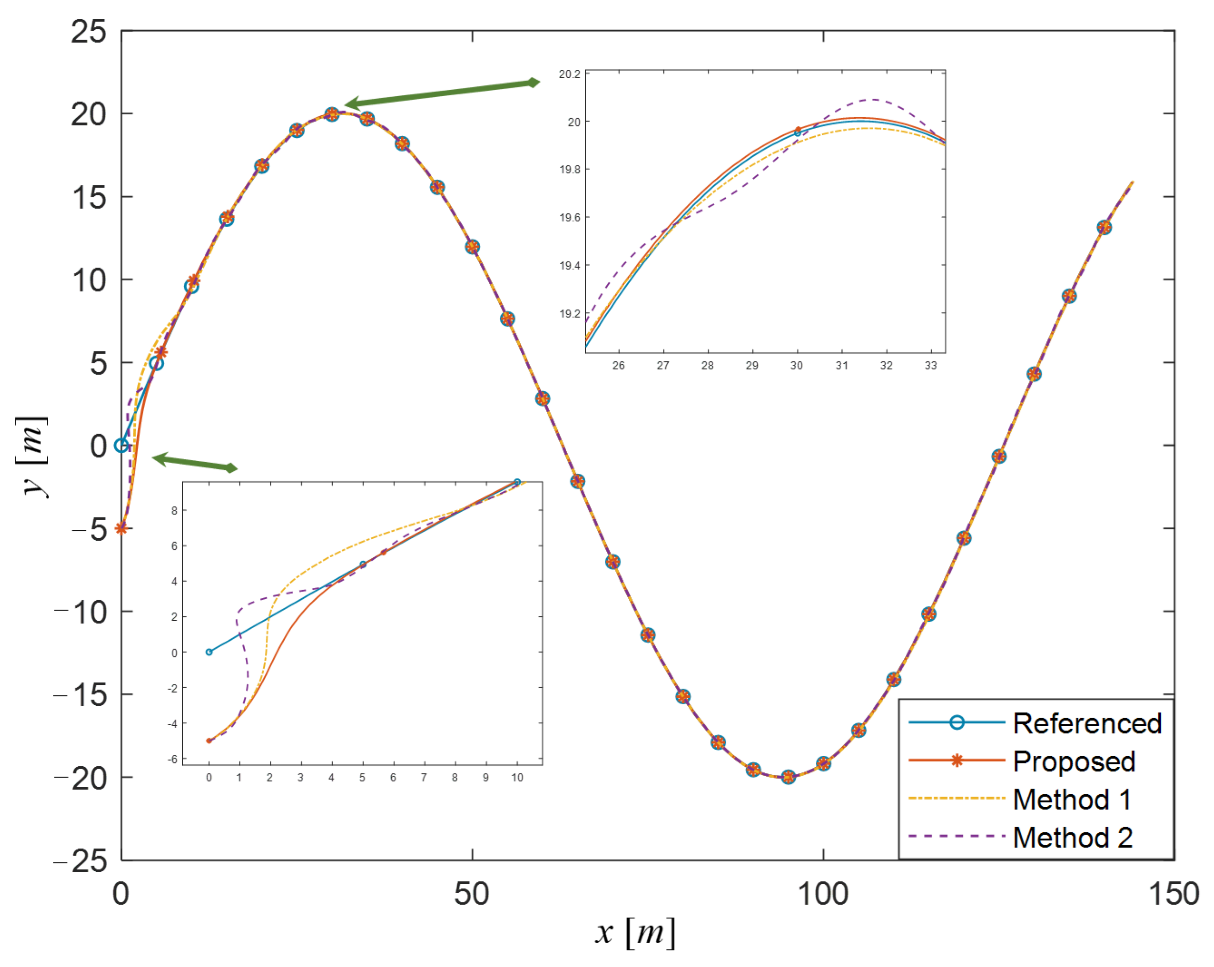
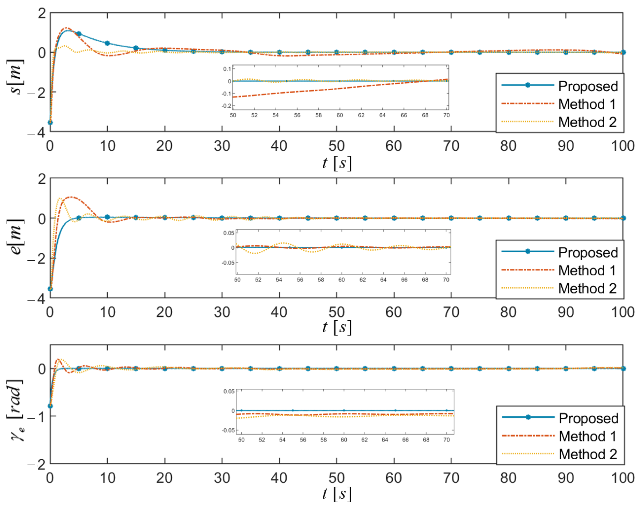
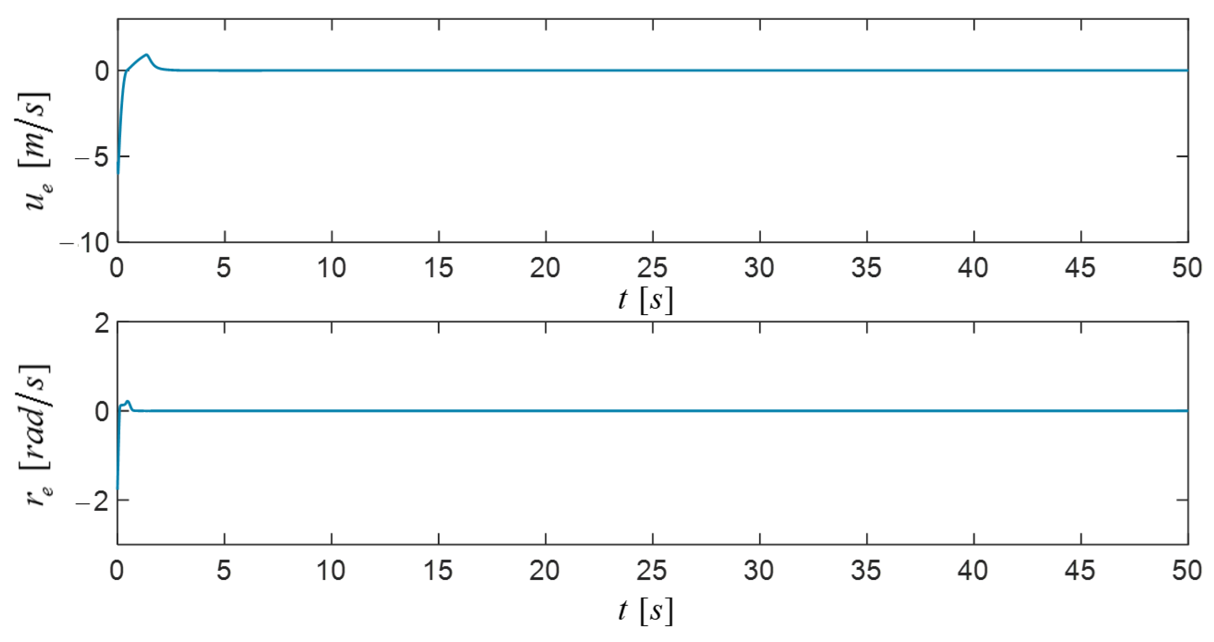
5.1. Case I: Sinusoidal Trajectory Tracking

In the horizontal plane, a sinusoidal referenced trajectory is set as follows:

$$p\left(t\right)=\left\{\begin{array}{cc}\hfill t,& \hfill 0\le \mathrm{t}\le 200\mathrm{s}\\ \hfill 20sin\left(0.05t\right),& \hfill 0\le \mathrm{t}\le 200\mathrm{s}\end{array}\right.$$

(65)

Set the initial pose as $\left[x\right(0),y(0),\psi (0),u(0),v(0),r(0\left)\right]$$=[0,0,-5,0,0,0]$. To verify the validity of the NAITSMC method, method 1 and method 2 are compared under the influence of CON-C to track Equation (65), and the X-AUV is impacted by environmental interferences as follows:

$$\begin{array}{cc}\hfill D_u& =0.1sin(0.05t+\frac{\pi }{3})-0.05sin\left(\frac{\pi }{10}\right)t\hfill \\ \hfill D_v& =0.2sin(0.04t+\frac{\pi }{3})-0.05sin\left(\frac{\pi }{10}\right)t\hfill \\ \hfill D_r& =0.2sin(0.05t+\frac{\pi }{3})-0.1sin\left(\frac{\pi }{10}\right)t\hfill \end{array}$$

(66)

Figure 5 shows that three methods were performed under the influence of CON-C. Although all the control methods could complete the mission, the NAITSMC method had excellent performance in CON-C, especially in the initial position and the corner of larger curvature which are pointed out as subfigures in Figure 5. Additionally, the NAITSMC method was not rushing to track the referenced trajectory without overshoot and required less time to get to the steady state compared with method 1 and method 2.

The tracking errors of Case I under the influence of CON-C are depicted, as shown in Figure 6. As we can see, the NAITSMC method had a quick response to achieve the steady state, and had robust performance in the CON-C environment. To show the specific efficiency of the proposed method, the results of tracking errors in steady state are reported in

Table 3. The specific data of tracking errors under CON-C.

	Ave. $\left|\mathit{s}\right|$	Ave. $\left|\mathit{e}\right|$	Ave. of $|{\mathbf{\chi }}_{\mathit{e}}|$	Var. of s	Var. of e	Var. of ${\mathbf{\chi }}_{\mathit{e}}$
Proposed	$5.78\times {10}^{-4}$	$6.96\times {10}^{-4}$	$6.93\times {10}^{-5}$	$3.94\times {10}^{-6}$	$5.77\times {10}^{-6}$	$6.68\times {10}^{-9}$
Method 1	$8.53\times {10}^{-2}$	$1.41\times {10}^{-2}$	$7.50\times {10}^{-3}$	$1.25\times {10}^{-2}$	$3.85\times {10}^{-4}$	$8.11\times {10}^{-5}$
Method 2	$7.10\times {10}^{-3}$	$2.26\times {10}^{-2}$	$1.15\times {10}^{-2}$	$1.36\times {10}^{-4}$	$1.49\times {10}^{-3}$	$1.88\times {10}^{-4}$

. The average absolute value (Ave.) and the variance value (Var.) of s, e, and ${\chi }_e$ are the least among the three approaches. The errors of virtual velocities were tracked accurately by the proposed method, as shown in Figure 7.

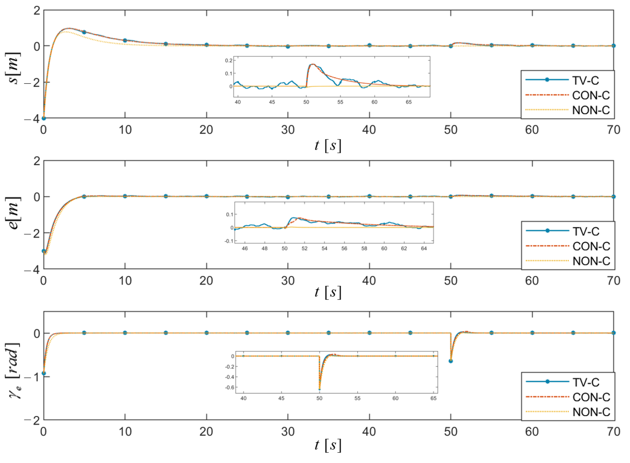
5.2. Case II: Compound Trajectory Tracking

In the horizontal plane, a compound referenced trajectory, which consisted of a line and a circle, was set as follows:

$$\begin{array}{c}\hfill x_d=\left\{\begin{array}{cc}\hfill 0.6t,& \hfill t\le 50\mathrm{s}\\ \hfill 70-40cos\left(0.05\right(t-50\left)\right),& \hfill 50<t\le 145\mathrm{s}\end{array}\right.\\ \hfill y_d=\left\{\begin{array}{cc}\hfill 0.8t,& \hfill t\le 50\mathrm{s}\\ \hfill 40+40sin\left(0.05\right(t-50\left)\right),& \hfill 50<t\le 145\mathrm{s}\end{array}\right.\end{array}$$

(67)

The initial pose was also set as $\left[x\right(0),y(0),\psi (0),u(0),v(0),r(0\left)\right]$$=[0,0,-5,0,0,0]$. After the numerical simulations of Case I, we aimed to verify the robustness and adaptability of the NAITSMC method under the influence of a TV-C environment, and the X-AUV is impacted by the environmental interferences in Equation (66).

Figure 8 shows that the different methods were performed under the influence of a TV-C environment. Although all the control methods could track the referenced trajectory, the NAITSMC method performed stably in the TV-C environment, especially in the initial position and the turning of curvature, which are pointed out as subfigures in Figure 8. Additionally, the NAITSMC method was not rushing to track the referenced trajectory without overshoot, and costed a little time to get the steady state compared with method 1 and method 2.

The tracking errors of the NAITSMC method under the influence of a NON-C environment, a CON-C environment, and a TV-C environment are depicted to verify the robustness and adaptability, as shown in Figure 9. As we can see, whatever ocean currents influence, the NAITSMC method can always complete the mission. There is no doubt that the NAITSMC method performed best in the TV-C environment. The results of the CON-C environment are basically the same as the results of the TV-C environment; therefore, the NAITSMC method can reduce environmental impacts, such as white Gaussian noise, compensated by RESO. The observations of RESO under the CON-C environment and TV-C environment are concluded in Figure 10. The results show that both unknown ocean currents CON-C and TV-C were estimated by RESO accurately.

To show the specific efficiency of the proposed scheme in different ocean current environments, the results of tracking errors in steady state were calculated, as shown in

Table 4. The specific data of tracking errors under in Case II.

	Ave. $\left|\mathit{s}\right|$	Ave. $\left|\mathit{e}\right|$	Ave. of $|{\mathbf{\chi }}_{\mathit{e}}|$	Var. of s	Var. of e	Var. of ${\mathbf{\chi }}_{\mathit{e}}$
Under TV-C	$3.90\times {10}^{-3}$	$4.30\times {10}^{-3}$	$1.94\times {10}^{-4}$	$1.67\times {10}^{-4}$	$2.01\times {10}^{-4}$	$2.37\times {10}^{-7}$
Under CON-C	$4.20\times {10}^{-4}$	$6.20\times {10}^{-4}$	$1.94\times {10}^{-4}$	$5.45\times {10}^{-5}$	$1.05\times {10}^{-5}$	$2.36\times {10}^{-7}$
Under NON-C	$1.91\times {10}^{-4}$	$1.92\times {10}^{-4}$	$1.95\times {10}^{-4}$	$2.29\times {10}^{-7}$	$2.31\times {10}^{-7}$	$2.38\times {10}^{-7}$

. The proposed method performs efficiently under difference environments to form a similar average of absolute values s, e, and ${\chi }_e$. However, the variances of s, e, and ${\chi }_e$ are differential because the influence of TV-C environment can only be predicted approximately. The errors of virtual velocity, which are tracked accurately, are described in Figure 11.

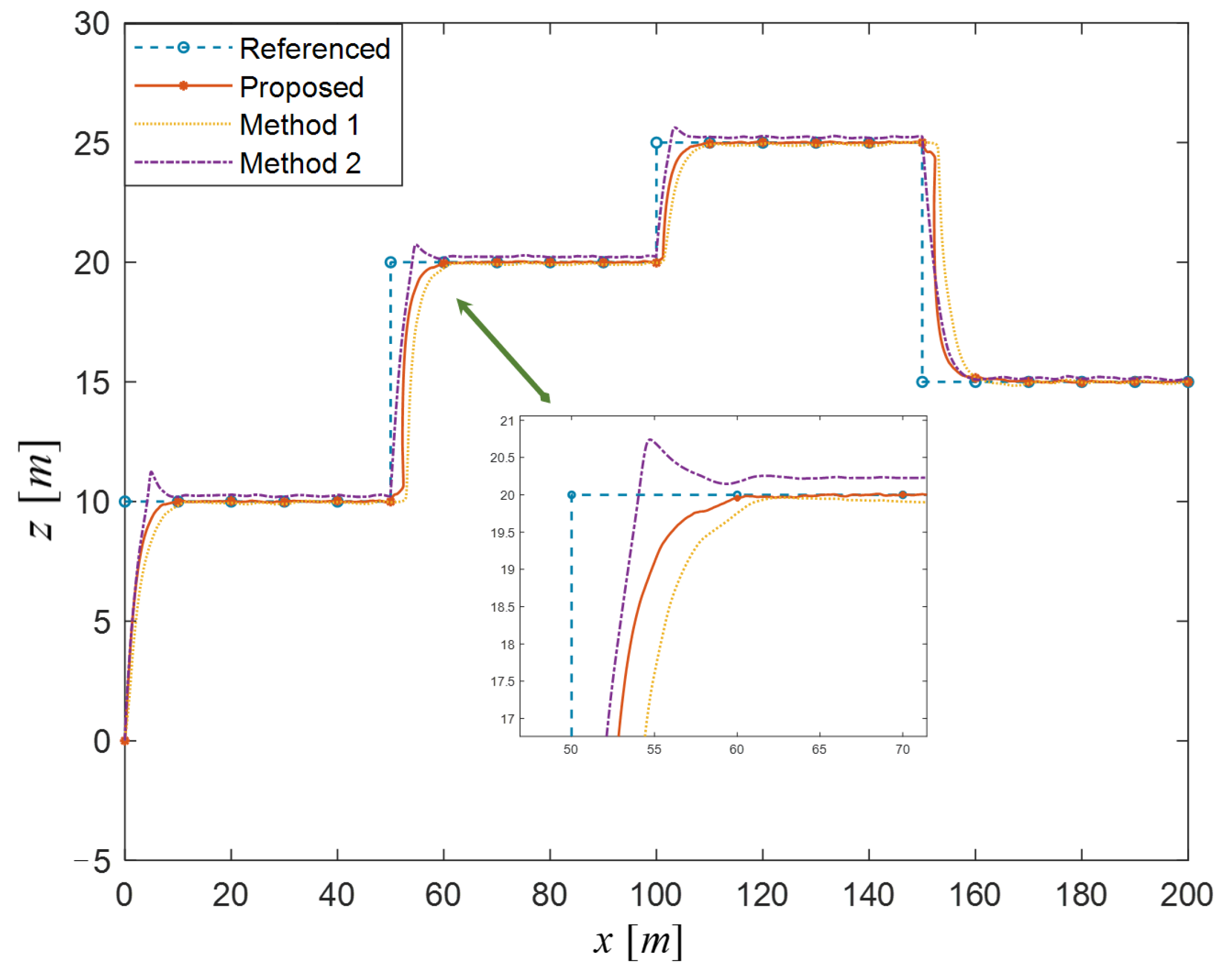
5.3. Case III: Trajectory Tracking of Variable Depth

In the vertical plane, a variable depth referenced trajectory is set as follows:

$$p\left(t\right)=\left\{\begin{array}{cc}10,& 0\le \mathrm{t}<50\mathrm{s}\\ 20,& 50\le \mathrm{t}<100\mathrm{s}\\ 25,& 100\le \mathrm{t}<150\mathrm{s}\\ 15,& 150\le \mathrm{t}<200\mathrm{s}\end{array}\right.$$

(68)

The initial pose is set as $\left[x\right(0),w(0),\theta (0),u(0),w(0),q(0\left)\right]$$=[0,0,0,0,0,0]$. To verify the validity of the NAITSMC method in the vertical plane, method 1 and method 2 are compared under the influence of the VT-C environment to track Equation (68), and the X-AUV is impacted by environmental interferences as follows:

$$\begin{array}{cc}\hfill D_u& =0.1sin(0.1t+\frac{\pi }{3})-0.05sin\left(\frac{\pi }{10}\right)t\hfill \\ \hfill D_w& =0.2sin(0.1t+\frac{\pi }{3})-0.05sin\left(\frac{\pi }{10}\right)t\hfill \\ \hfill D_q& =0.2sin(0.1t+\frac{\pi }{3})-0.1sin\left(\frac{\pi }{10}\right)t\hfill \end{array}$$

(69)

Figure 12 shows that three methods were performed under the influence of the VT-C environment. Although all the control methods could complete the mission, the NAITSMC method had an excellent performance in the depth changed positions, which are pointed out as subfigures in Figure 12. Additionally, the NAITSMC method was not rushing to track the referenced trajectory and had a smaller settling time. However, method 1 has some overshoot, and method 2 cost more time to get to the steady state compared with the proposed method. The specific data are shown in

Table 5. The specific data of tracking errors under TV-C.

	Ave. $\left|\mathit{s}\right|$	Ave. $\left|\mathit{h}\right|$	Ave. of $|{\mathbf{\upsilon }}_{\mathit{e}}|$	Var. of s	Var. of h	Var. of ${\mathbf{\upsilon }}_{\mathit{e}}$
Proposed	$4.93\times {10}^{-2}$	$1.18\times {10}^{-1}$	$3.30\times {10}^{-4}$	$4.55\times {10}^{-2}$	$0.56\times {10}^0$	$1.01\times {10}^{-5}$
Method 1	$3.78\times {10}^{-1}$	$5.39\times {10}^{-1}$	$3.76\times {10}^{-3}$	$1.45\times {10}^{-1}$	$2.36\times {10}^0$	$5.81\times {10}^{-4}$
Method 2	$1.23\times {10}^{-1}$	$4.88\times {10}^{-1}$	$2.25\times {10}^{-3}$	$1.05\times {10}^{-1}$	$1.49\times {10}^0$	$2.01\times {10}^{-4}$

.

6. Conclusions

In this research, the proposed scheme was introduced to reduce the problems of chattering, parameter perturbation, and time-varying disturbances in decoupled planes for the X-AUV. Firstly, the kinematics control law is designed based on the compound orientation angle. After that, the dynamic control law based on the NAITSMC method was designed by the Lyapunov stability theorem with the adaptive law to solve unknown environmental interferences. Considering the influences of time-varying ocean currents, the RESO is introduced to compensate for the model-based of ocean currents described by the first-order Gauss–Markov process. Additionally, the whole system was verified as global asymptotic stability. Finally, the results show that the proposed scheme has robustness and adaptability in decoupled planes.

Furthermore, we will extend the proposed scheme to perform real experiments in lakes or oceans, and further explore the selection of controller parameters in the experiment.

References

1. Lv, T.; Zhang, M.; Wang, Y. Prediction-Based Region Tracking Control Scheme for Autonomous Underwater Vehicle. J. Mar. Sci. Eng. 2022, 10, 775. [Google Scholar] [CrossRef]
2. Liu, Z.; Cai, W.; Zhang, M.; Lv, S. Improved Integral Sliding Mode Control-Based Attitude Control Design and Experiment for High Maneuverable AUV. J. Mar. Sci. Eng. 2022, 10, 795. [Google Scholar] [CrossRef]
3. Li, D.; Du, L. Auv trajectory tracking models and control strategies: A review. J. Mar. Sci. Eng. 2021, 9, 1020. [Google Scholar] [CrossRef]
4. Miao, J.; Wang, S.; Zhao, Z.; Li, Y.; Tomovic, M.M. Spatial curvilinear path following control of underactuated AUV with multiple uncertainties. ISA Trans. 2017, 67, 107–130. [Google Scholar] [CrossRef]
5. Fang, Y.; Pu, J.; Yuan, C.; Cao, Y.; Liu, S. A control strategy of normal motion and active self-rescue for autonomous underwater vehicle based on deep reinforcement learning. AIP Adv. 2022, 12, 015219. [Google Scholar] [CrossRef]
6. Aguiar, A.P.; Hespanha, J.P. Trajectory-tracking and path-following of underactuated autonomous vehicles with parametric modeling uncertainty. IEEE Trans. Autom. Control 2007, 52, 1362–1379. [Google Scholar] [CrossRef] [Green Version]
7. Roy, S.; Shome, S.; Nandy, S.; Ray, R.; Kumar, V. Trajectory following control of AUV: A robust approach. J. Inst. Eng. (India) Ser. C 2013, 94, 253–265. [Google Scholar] [CrossRef]
8. Jiang, Y.; Guo, C.; Yu, H. Robust trajectory tracking control for an underactuated autonomous underwater vehicle based on bioinspired neurodynamics. Int. J. Adv. Robot. Syst. 2018, 15, 1729881418806745. [Google Scholar] [CrossRef] [Green Version]
9. Elmokadem, T.; Zribi, M.; Youcef-Toumi, K. Terminal sliding mode control for the trajectory tracking of underactuated Autonomous Underwater Vehicles. Ocean Eng. 2017, 129, 613–625. [Google Scholar] [CrossRef]
10. Yu, C.; Xiang, X.; Lapierre, L.; Zhang, Q. Nonlinear guidance and fuzzy control for three-dimensional path following of an underactuated autonomous underwater vehicle. Ocean Eng. 2017, 146, 457–467. [Google Scholar]
11. Patre, B.; Londhe, P.; Waghmare, L.; Mohan, S. Disturbance estimator based non-singular fast fuzzy terminal sliding mode control of an autonomous underwater vehicle. Ocean Eng. 2018, 159, 372–387. [Google Scholar] [CrossRef]
12. Kim, E.; Fan, S.; Bose, N.; Nguyen, H. Current estimation and path following for an autonomous underwater vehicle (AUV) by using a high-gain observer based on an AUV dynamic model. Int. J. Control. Autom. Syst. 2021, 19, 478–490. [Google Scholar] [CrossRef]
13. Liang, X.; Qu, X.; Hou, Y.; Ma, Q. Three-dimensional trajectory tracking control of an underactuated autonomous underwater vehicle based on ocean current observer. Int. J. Adv. Robot. Syst. 2018, 15, 1729881418806811. [Google Scholar] [CrossRef]
14. Miao, J.; Wang, S.; Tomovic, M.M.; Zhao, Z. Compound line-of-sight nonlinear path following control of underactuated marine vehicles exposed to wind, waves, and ocean currents. Nonlinear Dyn. 2017, 89, 2441–2459. [Google Scholar] [CrossRef]
15. Yu, C.; Xiang, X.; Wilson, P.A.; Zhang, Q. Guidance-error-based robust fuzzy adaptive control for bottom following of a flight-style AUV with saturated actuator dynamics. IEEE Trans. Cybern. 2019, 50, 1887–1899. [Google Scholar] [CrossRef] [Green Version]
16. Rezazadegan, F.; Shojaei, K.; Sheikholeslam, F.; Chatraei, A. A novel approach to 6-DOF adaptive trajectory tracking control of an AUV in the presence of parameter uncertainties. Ocean Eng. 2015, 107, 246–258. [Google Scholar] [CrossRef]
17. Wang, W.; Xia, Y.; Chen, Y.; Xu, G.; Chen, Z.; Xu, K. Motion control methods for X-rudder underwater vehicles: Model based sliding Mode and non-model based iterative sliding mode. Ocean Eng. 2020, 216, 108054. [Google Scholar] [CrossRef]
18. Xia, Y.; Xu, K.; Huang, Z.; Wang, W.; Xu, G.; Li, Y. Adaptive energy-efficient tracking control of a X rudder AUV with actuator dynamics and rolling restriction. Appl. Ocean Res. 2022, 118, 102994. [Google Scholar] [CrossRef]
19. Fang, Y.; Huang, Z.; Pu, J.; Zhang, J. AUV position tracking and trajectory control based on fast-deployed deep reinforcement learning method. Ocean Eng. 2022, 245, 110452. [Google Scholar] [CrossRef]
20. Liu, X.; Zhang, M.; Rogers, E. Trajectory tracking control for autonomous underwater vehicles based on fuzzy re-planning of a local desired trajectory. IEEE Trans. Veh. Technol. 2019, 68, 11657–11667. [Google Scholar] [CrossRef]
21. Fossen, T.I. Handbook of Marine Craft hydrodynamics and Motion Control; John Wiley & Sons: Hoboken, NJ, USA, 2011. [Google Scholar]
22. Yu, H.; Guo, C.; Yan, Z. Globally finite-time stable three-dimensional trajectory-tracking control of underactuated UUVs. Ocean Eng. 2019, 189, 106329. [Google Scholar] [CrossRef]
23. Rout, R.; Subudhi, B. Inverse optimal self-tuning PID control design for an autonomous underwater vehicle. Int. J. Syst. Sci. 2017, 48, 367–375. [Google Scholar] [CrossRef]
24. Xia, Y.; Xu, K.; Wang, W.; Xu, G.; Xiang, X.; Li, Y. Optimal robust trajectory tracking control of a X-rudder AUV with velocity sensor failures and uncertainties. Ocean Eng. 2020, 198, 106949. [Google Scholar] [CrossRef]
25. Yu, C.; Liu, C.; Xiang, X.; Zeng, Z.; Wei, Z.; Lian, L. Line-of-sight guided time delay control for three-dimensional coupled path following of underactuated underwater vehicles with roll dynamics. Ocean Eng. 2020, 207, 107410. [Google Scholar] [CrossRef]
26. Zhang, Y.; Li, Y.; Sun, Y.; Zeng, J.; Wan, L. Design and simulation of X-rudder AUV’s motion control. Ocean Eng. 2017, 137, 204–214. [Google Scholar] [CrossRef]
27. Li, Y.; Wang, X.; Zhang, J.; Cao, J.; Zhang, Y. X-Rudder Autonomous Underwater Vehicle Control Allocation Based on Improved Quadratic Programming Algorithm. J. Shanghai Jiaotong Univ. 2020, 54, 524. [Google Scholar]
28. Shengda, S. Submarine Maneuverability; National Defense Industry Press: Beijing, China, 1995; Volume 30–45. [Google Scholar]
29. Repoulias, F.; Papadopoulos, E. Planar trajectory planning and tracking control design for underactuated AUVs. Ocean Eng. 2007, 34, 1650–1667. [Google Scholar] [CrossRef]
30. Xue, W.; Huang, Y. On performance analysis of ADRC for a class of MIMO lower-triangular nonlinear uncertain systems. ISA Trans. 2014, 53, 955–962. [Google Scholar] [CrossRef] [PubMed]
31. Breivik, M.; Fossen, T.I. Principles of guidance-based path following in 2D and 3D. In Proceedings of the 44th IEEE Conference on Decision and Control, Seville, Spain, 15 December 2005; pp. 627–634. [Google Scholar]
32. Breivik, M.; Fossen, T.I. Guidance-based path following for autonomous underwater vehicles. In Proceedings of the OCEANS 2005 MTS/IEEE, Washington, DC, USA, 17–23 September 2005; pp. 2807–2814. [Google Scholar]
33. Roy, S.; Baldi, S.; Fridman, L.M. On adaptive sliding mode control without a priori bounded uncertainty. Automatica 2020, 111, 108650. [Google Scholar] [CrossRef]
34. Lei, Q.; Zhang, W. Adaptive non-singular integral terminal sliding mode tracking control for autonomous underwater vehicles. IET Control Theory Appl. 2017, 11, 1293–1306. [Google Scholar]
35. Li, Y.; Jiang, Y.q.; Ma, S.; Chen, P.y.; Li, Y.m. Inverse speed analysis and low speed control of underwater vehicle. J. Cent. South Univ. 2014, 21, 2652–2659. [Google Scholar] [CrossRef]
Figure 1. The description for different frames.
Jmse 10 01408 g001
Figure 2. The frame of trajectory tracking control.
Jmse 10 01408 g002
Figure 3. The definitions of trajectory tracking errors in the horizontal plane.
Jmse 10 01408 g003
Figure 4. The definitions of trajectory tracking errors in the vertical plane.
Jmse 10 01408 g004
Figure 5. The different methods under the influence of CON-C.
Jmse 10 01408 g005
Figure 6. The tracking errors with different methods under the influence of CON-C.
Jmse 10 01408 g006
Figure 7. The errors of virtual speed for the proposed method under the influence of CON-C.
Jmse 10 01408 g007
Figure 8. The different methods under the influence of TV-C.
Jmse 10 01408 g008
Figure 9. The tracking errors with NAITSMC methods under the influence of different currents.
Jmse 10 01408 g009
Figure 10. Unknown ocean current disturbances estimated by RESO.
Jmse 10 01408 g010
Figure 11. The errors of virtual speed for the proposed method under the influence of TV-C.
Jmse 10 01408 g011
Figure 12. The different methods under the influence of TV-C.
Jmse 10 01408 g012