Abstract
In this paper, a 2-stage cascaded deep learning framework, Port Wave Prediction Network (PWPNet), is proposed for real-time prediction of significant wave height (SWH) distribution in a port. The PWP-out model of the first stage, predicting port-entrance wave parameters, utilizes three branches, the first branch using a Long Short Term Memory (LSTM) module to learn the temporal dependencies of time sequences of port-entrance wave parameters, the second branch using Wave and Wind field Feature Extraction (WWFE) modules, composed of a residual network with spatial and channel attention, to capture spatiotemporal characteristics of outside-port 2D wave and wind field data, the third branch using multi-scale time encoding to capture the periodic characteristics of waves and wind. The PWP-in model of the second stage, estimating the in-port SWH distribution, uses port-entrance wave parameters based on a customized Artificial Neural Network (ANN) and takes PWP-out’s output as its input. A comparison of the performance of PWP-out and mainstream machine learning models including LSTM, GRU, BPNN, SVR, ELM, and RF at Hambantota Port shows that PWP-out outperforms all other models regarding medium-term (25–48 h), med–long-term (49–72 h), and long-term (73–96 h) predictions, and ablation experiments proved the effectiveness of the three branches. Furthermore, the performance comparison of our PWPNet and other 2-stage models of LSTM, GRU, BPNN, SVR, ELM, and RF cascaded with PWP-in shows that PWPNet outperforms those cascaded models for medium-term to long-term predictions of SWH distribution in a port.
1. Introduction
Ocean waves affect a variety of marine activities and people’s security. For example, the waves in a port caused the mooring ships to move excessively and made it impossible to unload cranes [1], which in turn affected the operation of Hambantota Port and the construction of the maritime Silk Road. Therefore, the research on a fast and reliable prediction method of significant wave height (SWH) in the port can help reduce the vibration of moored ships [2], and improve the port operation plan, and it is also very important for improving the safety of coastal engineering and shipping planning.
Numerical models are the most widely used methods in wave prediction, including the third-generation wave model WAM [3] that integrates the basic transport equations describing the evolution of the two-dimensional wave direction spectrum, the US global ocean wave operational forecast model Wavewatch III [4] developed on the basis of the WAM model, the phase-averaged wind wave model SWAN [5] based on a fully spectral representation of the action balance equation, the SWASH model based on nonlinear shallow water equations [6], and the FUNWAVE-TVD and MIKE21BW based on Boussinesq-type equations [7]. Wornom et al. [8] performed a simulation of wind–wave activity for the 1995 Hurricane Luis to determine the effect of applying SWAN in the inner WAM domain to obtain more accurate nearshore wave predictions. Choi et al. [9] predicted SWH in a port by using SWAN to simulate the propagation of outside-port wind waves and predict the boundary conditions for the FUNWAVE-TVD model and interpolate the SWH of FUNWAVE-TVD’s output in a port. However, numerical models require time-consuming calculation, especially for dense computational grids, and it is difficult to meet the needs of real-time nearshore wave prediction.
In recent years, machine-learning-based methods have become popular in wave prediction, which avoids complex calculation of numerical simulation and can be applied to real-time wave prediction. Ali et al. [10] combined Extreme Learning Machine (ELM) model and an Improved Complete Ensemble Empirical Mode Decomposition (ICEEMD) method to predict SWH at two coastal locations in Queensland, Australia, and obtained better prediction results than Online Sequence Extreme Learning Machine (OSELM) and Random Forest (RF). Kumar et al. [11] used Deep Belief Network (DBN) and transfer learning to predict wave states at observation stations in the Gulf of Mexico, South Korea, and the United Kingdom, and the prediction results were better than ELM, Support Vector Regression (SVR), and Minimal Resource Allocation Network (MRAN). Law et al. [12] used Artificial Neural Network (ANN) to predict short-term deterministic waves in southern Albany, achieving less than 20% error compared to the Linear Wave Theory (LWT)-based model. Demetriou et al. [13] used the structural wave acceleration data and wind field data for training ANN and decision tree models for real-time prediction of the coastal zone SWH. Currently, Recurrent Neural Network (RNN)-based methods are becoming more and more popular in wave prediction, mainly Long Short Term Memory (LSTM) and Gated Recurrent Unit (GRU). Fan et al. [14] used LSTM to predict buoy-observed SWH in the next 12 h, 1 day, 2 days, and 3 days, showing that LSTM has better prediction performance in these time spans than BP neural network, Support Vector Machine (SVM), Extreme Learning Machine (ELM), and RF. Then, Wang et al. [15] predicted buoy-observed SWH of six stations in the Taiwan Strait and its adjacent sea area in the next 3, 6, 12, and 24 h using the GRU model, and the prediction results were better than the BP neural network, SVM, and ELM.
Regarding wave predictions in a port, real-time prediction of the SWH distribution of the whole port has not been achieved yet. Gopinath et al. [16] used ANN and NARX network to predict the weekly and monthly average SWH of a single buoy in New Mangalore port on the west coast of India, however, these methods can only predict the SWH at a limited number of buoy locations. Zheng et al. [17] used the ANN model to estimate SWH at 12 positions in a port including a buoy and 11 berths using port-entrance wave parameters, however, this method relies on a numerical model providing port-entrance wave parameters to make in-port SWH predictions, so it is difficult to achieve real-time prediction.
To sum up, currently, numerical-model-based methods are not suitable for real-time prediction of in-port SWH, while machine-learning-based wave prediction methods mostly focus on limited locations of buoys with reasonable short-term prediction results. A high-quality real-time long-term prediction of in-port SWH distribution is conducive to the advanced plan for disaster prevention and port management and reduces personnel and economic losses. Therefore, it is urgent to develop an efficient method for real-time SWH distribution prediction of the whole port with better long-term prediction results.
This paper proposes a novel 2-stage deep learning framework called PWPNet for real-time prediction of SWH distribution in a port, composed of PWP-out and PWP-in. PWP-out predicts port-entrance wave parameters, and PWP-in estimates in-port SWH distribution using PWP-out’s output. Section 2 introduces the datasets and processing for PWPNet. Section 3 describes the overall structure and detailed parts of PWPNet. Section 4 shows experiments and results of PWPNet. Section 5 discusses the performance of PWPNet and data availability. Section 6 concludes the paper.
2. Datasets and Processing
In order to build the 2-stage cascaded neuron network PWPNet, two datasets need to be built for training and testing in each stage. The first dataset is called the outside-port 2D wave and wind field dataset, containing the collected outside-port 2D wave and wind field data over recent years, used for training and testing PWP-out. The second dataset is called the in-port SWH dataset, containing SWH distribution data of a port generated by a numerical model, used for training and testing PWP-in.
2.1. Collect the Outside-Port 2D Wave and Wind Field Dataset
We chose the Hambantota Port of Sri Lanka as the target port. Its longitude and latitude are 81.0921°E and 6.1315°N, respectively. The outside-port 2D wave and wind field data are from the ERA5 hourly reanalysis dataset on single levels [18] (referred to as the ERA5 dataset) from the European Centre for Medium-Range Weather Forecasts (ECMWF) from 2010 to 2020. The longitude range of the ERA5 dataset is 64° E–96° E, the latitude range is 11° S–21° N, and the geographical resolution is 0.5° × 0.5°. In other words, there are 64 × 64 grids with a 1 h time interval.
This dataset is built for prediction of port-entrance wave parameters including significant wave height (SWH), peak wave period (PP1D), mean wave direction (MWD), and wave directional spectrum width (WDW), so these four wave attributes were collected for the dataset. Wave height is generally considered to be influenced by historical wave height, the wind direction and speed [19]. Therefore, we collected wind attributes too, including the east–west component of wind speed at 10 m above sea level (U10) and the north–south component of wind speed at 10 m above sea level (V10).
2.2. Generate the In-Port SWH Dataset Using the Calibrated SWASH Model
We obtained two buoy-observed SWH datasets (ADCP1 in the port and ADCP2 at the port entrance) collected by Zheng et al. [17]. The location and observation periods of the buoys are labeled in Figure 1. However, the buoy-observed SWH dataset contains only the time sequences of SWH at the buoy location, which cannot meet the requirements of training a deep neuron network for in-port SWH distribution estimation. Moreover, the cost and maintenance of buoys are expensive. Therefore, we used the SWASH (Simulating WAves till Shore) model calibrated by ADCP1-observed SWH data to generate the in-port SWH dataset. The SWASH model is a numerical model for simulating non-hydrostatic, free-surface, rotational flows, based on nonlinear shallow water equations [6], and it can simulate the diffraction and reflection propagation of waves in a port. The detailed parameter settings of the SWASH model are as follows.
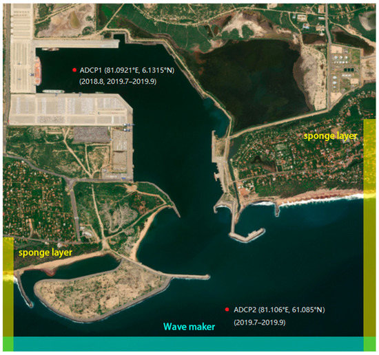
Figure 1.
Setting of the wave maker and sponge layers.
The compute domain is 3840 × 3840 m, the size of the computational grid is 5 × 5 m, and the wave maker is in the south of the compute domain with a weak reflective boundary condition [20]. The wave maker takes port-entrance wave parameters including SWH, PP1D, MWD, and WDW as inputs to propagate a wave over the whole port. The JONSWAP spectrum [21] is used considering that the water depth of the whole port is around 17 m, while the port-entrance SWH is concentrated in 1–2.5 m, which is approximately regarded as the case of deep water. The distribution function is and the directional width is expressed with the power m. In order to prevent wave reflection on the side of the wave maker, sponge layers with a width of 40 m are added to the eastern and western sides, as shown in Figure 1. We chose the Manning formula [22] with a coefficient of 0.002 to deal with friction at the bottom of the port. For efficient computation, we used one vertical layer. The default wave breaking method in SWASH is a depth-induced wave breaking model [23,24]. We set wave breaking 23 coefficients α = 0.8, β = 0.15 to handle wave breaking, and we used a MUSCL limiter [25] to ensure non-negative water depth. The porosity of port structures was set to 1, and that of sea area was set to 0.025. The timestep for time integration was set to 0.1 s and the Courant–Friedrichs–Lewy (CFL) condition [26] was used to dynamically change the timestep for faster calculations, with a minimum number of 0.1 and a maximum number of 0.5. The total simulation time was 3000 s. After 1800 s, the wave conditions in the port were almost stable, so the time period of 1800–3000 s was chosen for SWH calculation. The formula of SWH is shown in Formula (1), where is the calculated SWH, E(f) is the variance density spectrum, and f is the frequency.
As shown in Figure 2, we made comparisons of the data generated by the calibrated SWASH model at the ADCP1 location at each hour of the buoy observation (the horizontal axis) and the buoy-observed data of each hour (the vertical axis) including SWH and PP1D, and they are roughly consistent. MAE is the mean absolute error, RMSE is the root mean square error, and PCC is the Pearson correlation coefficient. We did not compare wave direction because ADCP1 is located in the inner port, where waves experience diffraction and reflection many times, leading to complex composition and rapid changes in the mean wave direction (MWD), so comparison with buoy-observed MWD would be unhelpful. Therefore, the calibrated SWASH model can be used for in-port SWH dataset generation.
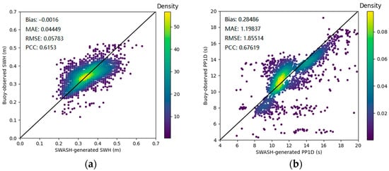
Figure 2.
Comparisons between the buoy-observed data and the SWH (a) and PP1D (b) generated by the calibrated SWASH model at the ADCP1 location.
In order to generate the in-port SWH dataset using the calibrated SWASH model, a variety of port-entrance wave parameters (SWH, PP1D, MWD, and WDW) were uniformly sampled from the ERA5 dataset in the time period of 2010–2020 at the entrance of the Hambantota Port as the inputs of the calibrated SWASH model for in-port SWH dataset generation. To validate the usability of ERA5 dataset at the port entrance, we compared the ADCP2-observed SWH and the SWH of ERA5 at the ADCP2 location interpolated by cubic spline interpolation, and the comparison result is shown in Figure 3. Finally, a total of 384 samples were obtained, as shown in Table 1.
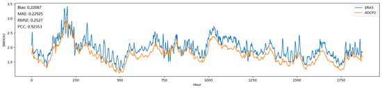
Figure 3.
Comparison of the ADCP2-observed SWH and interpolated SWH from ERA5.

Table 1.
Port-entrance wave parameters required to generate the in-port SWH dataset using the calibrated SWASH model.
3. Proposed Model: PWPNet
As shown in Figure 4, PWPNet is a 2-stage deep neuron network cascaded by the port-entrance wave parameters prediction model PWP-out and in-port SWH distribution estimation model PWP-in. PWP-out predicts the future N-timestep sequences of port-entrance wave parameters. PWP-in takes port-entrance wave parameters predicted by PWP-out as input, to estimate in-port SWH distribution (represented as an image with a resolution of H′ × W′) of these N-timestep sequences. In Section 3.1 and Section 3.2, PWP-out and PWP-in will be described in detail, respectively.
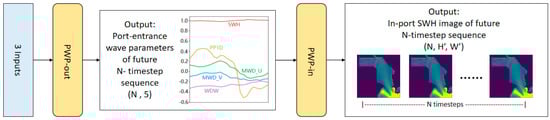
Figure 4.
PWPNet structure diagram.
3.1. Port-Entrance Wave Parameters Prediction Model: PWP-Out
3.1.1. Overall Structure of PWP-Out
As shown in Figure 5, PWP-out is a neural network composed of three branches corresponding to three inputs. In the first branch, historical M-timestep sequences of port-entrance wave parameters are input into LSTM module to learn the temporal dependencies of time sequences of port-entrance wave parameters. LSTM [27] is a special Recurrent Neural Network (RNN), which uses gates to control data transmission states, and solves the problem of gradient vanishing and gradient exploding in long sequence training. In the second branch, historical M-timestep sequences of the outside-port 2D wave and wind field data with a resolution of H × W are input into Wave and Wind field Feature Extraction (WWFE) modules, and then through a full connection layer and an ReLU activation function shown in Formula (2), to capture the spatiotemporal characteristics of the outside-port 2D wave and wind field. In the third branch, the multi-scale time encoding of the current timestep captures the periodic characteristics of waves and winds. Then, the outputs of the three branches are concatenated and passed into the stacked fully connected layers to output prediction results of future N-timestep sequences of port-entrance wave parameters.
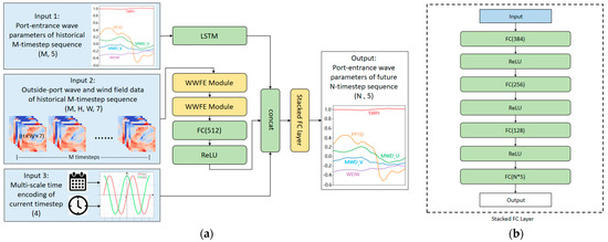
Figure 5.
PWP-out structure diagram, where (a) is the overall structure and (b) is the stacked FC layer of (a).
The two key components in PWP-out, including WWFE module and multi-scale time encoding, are described in Section 3.1.2 and Section 3.1.3 respectively.
3.1.2. WWFE Module in PWP-Out
The Wave and Wind field Feature Extraction (WWFE) module is incorporated in PWP-out, which consists of channel attention and spatial attention. Figure 6 shows the structure of the WWFE module. Spatial attention aims to make the network pay attention to outside-port locations where wave conditions have an influence on the port-entrance wave parameters, and channel attention aims to make the network pay attention to outside-port wave attributes which have an influence on port-entrance wave parameters. Moreover, the WWFE module uses a residual network [28] to reduce gradient vanishing. The WWFE module outputs feature images with half resolution compared to the input, to extract features from the outside-port 2D wave and wind field to lower dimensions.
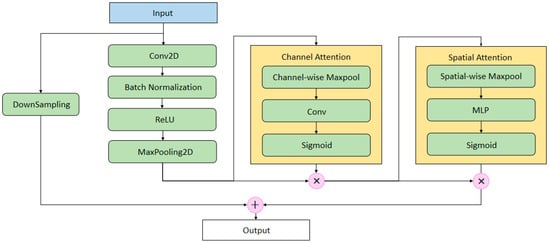
Figure 6.
Structure diagram of the Wave and Wind field Feature Extraction (WWFE) module.
3.1.3. Multi-Scale Time Encoding in PWP-Out
Based on sin-cos encoding, a multi-scale time encoding of the current timestep is encoded into a vector with a dimension of 4. Months and hours are encoded into two-dimensional vectors, as shown in Formulas (3)–(6). Sin-cos encoding is better than one-hot encoding because sin and cos functions are consistent. Using both sin and cos functions also ensures that each encoding is unique, avoiding the problem that a single sin(x) or cos(x) value corresponds to more than one x value in a period. Thus, it is easier to capture periodic characteristics of waves and wind.
3.2. In-Port SWH Estimation Model: PWP-In
The in-port SWH estimation model PWP-in is a customized Artificial Neural Network (ANN), as shown in Figure 7, which consists of an input layer, 2–3 hidden layers, and an output layer. The activation function of the output layer is set to Tanh to limit the output between −1 and 1, and the activation functions of the hidden layers are set to ReLU. The formula of the Tanh function is shown in Formula (7). The number of neurons in the input layer is 5, corresponding to the number of port-entrance wave parameters (SWH, PP1D, MWD_U, MWD_V, and WDW), and the number of neurons in the output layer is equal to the total number of pixels of the estimated SWH image. The output layer is reshaped into H′ × W′ (256 × 256) grids and multiplied by the port mask to show the SWH image of the port. Here, the port mask is used to distinguish the port from the land. The port area is set to 1 and the land area is set to 0.
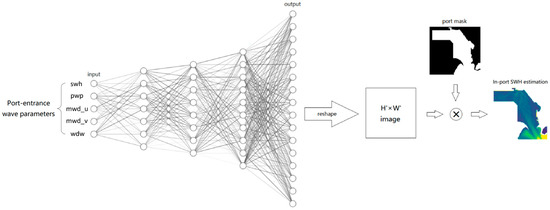
Figure 7.
Structure diagram of PWP-in.
4. Experiments and Analysis
4.1. Experiments of PWP-Out on the Outside-Port 2D Wave and Wind Field Dataset
In this paper, the outside-port 2D wave and wind field dataset mentioned in Section 2.1 was selected as the PWP-out experimental dataset, where the resolution of outside-port 2D wave and wind field dataset (H × W) was set to 64 × 64. The training set covers a time period of 2010–2019 and the test set covers 2020. As for the PWP-out hyper-parameter settings, historical timesteps M was set to 6, and future timesteps N was set to 24. We set the batch size to 512, the optimizer to Adam, the learning rate to 0.002, and number of epochs to 100. The training of PWP-out was carried out on an NVIDIA RTX 3080 GPU.
In order to test the performance of our model, we carried out the comparison experiment of PWP-out, LSTM, GRU, BPNN, SVR, ELM, and RF, as well as the ablation experiment of PWP-out itself. We used mean absolute error (MAE), mean absolute percentage error (MAPE), root mean square error (RMSE), and correlation coefficient () to evaluate the prediction accuracy of these five wave parameters (SWH, PP1D, MWD_U, MWD_V, and WDW). The formulas of MAE, MAPE, RMSE, and are shown in Formulas (8)–(11), where n is the number of samples, is the ground truth of the ith sample, is the predicted value of the ith sample, is the average of the ground truths, and is the average of the predicted values. For MAE, MAPE, and RMSE, lower values mean higher accuracy, while for higher values mean a higher correlation.
4.1.1. Comparison Experiment
In the comparison experiment, the prediction performance of port-entrance wave parameters was tested between PWP-out and six other methods (LSTM, GRU, BPNN, SVR, ELM, and RF). The three inputs of PWP-out included historical port-entrance wave parameters, outside-port 2D wave and wind field data, and multi-scale time encoding, while the input of six other methods was historical port-entrance wave parameters only.
The prediction performance of PWP-out and six other methods at different time spans is displayed in Figure 8 using small charts. These charts cover five wave parameters (SWH, PP1D, MWD_U, MWD_V, and WDW) from top to bottom, and four metrics (MAE, MAPE, RMSE, and ) from left to right. Each chart includes short-term prediction (1–24 h), medium-term prediction (25–48 h), med–long-term prediction (49–72 h), and long-term prediction (72–96 h) results.
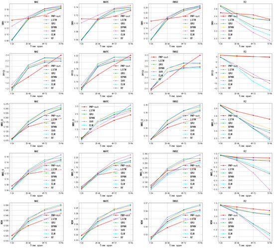
Figure 8.
Performance comparison between PWP-out and other models.
It can be seen that the prediction accuracy of PWP-out is generally better than all other models except in short-term prediction. PWP-out does not perform as well as other methods in short-term prediction, most likely because the wave conditions usually do not change significantly in a short time period, thus, using only time sequences of port-entrance wave parameters causes relatively small prediction errors. As the time span for prediction increases, the impact of the outside-port 2D wave and wind field on future waves becomes more prominent, so PWP-out can more accurately predict the port-entrance wave parameters and has obvious advantage over mainstream prediction methods which only utilize the historical port-entrance wave parameters.
4.1.2. Ablation Experiment
The ablation experiment was conducted to prove the effectiveness of the three branches in PWP-out. The PWP-out structure without port-entrance wave parameter input and its branch is called PWP-out-E, the PWP-out structure without outside-port 2D wave and wind field data input and its branch is called PWP-out-O, and the PWP-out structure without multi-scale time encoding input and its branch is called PWP-out-T. The results of ablation experiments are shown in Figure 9.
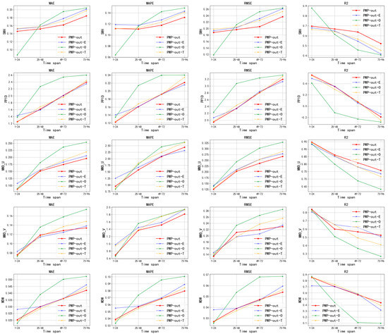
Figure 9.
Performance comparison between PWP-out and other ablated models.
It can be seen that PWP-out is generally better than other ablated models in medium-term (25–48 h), med–long-term (49–72 h), and long-term (73–96 h) predictions. Some analyses of the results are presented here:
- PWP-out performs better than PWP-out-E overall, because PWP-out captures temporal dependencies of time sequences of port-entrance wave parameters to predict more accurately.
- PWP-out-O performs the best in short-term prediction (1–24 h) in the ablation experiment, because outside-port 2D wave and wind field has little correlation with short-term prediction results, thus, avoiding this input significantly improves short-term prediction performance.
- PWP-out performs better than PWP-out-T overall, because Hambantota Port is affected by monsoon according to [29], the weather and climate of Sri Lanka is dominated by the monsoons, Southwest Monsoon (SWM) from May to September and Northeast Monsoon (NEM) from December to February, showing significant yearly periodicity. Additionally, the sea–land thermal contrast plays a role in the formation of monsoons, showing daily periodicity. As a result, the multi-scale time encoding improves prediction performance.
4.2. Experiments of PWP-In on the In-Port SWH Dataset
As described in Section 2.2, the in-port SWH dataset was used for training and testing PWP-in. We used an NVIDIA RTX 3080 GPU for training PWP-in.
In order to customize the optimal ANN structure (number of layers and the number of neurons in each layer) of PWP-in, we tested the following eight ANN structures. The No. 1–No. 4 cases were set to five layers, and the No. 5–No. 8 were set to four layers. The number of neurons of the output layer of these eight structures was the same, 65,536, to stay consistent with the SWH image resolution of the port (H′ × W′, 256 × 256). The number of neurons corresponding to each layer is shown in Table 2.
Table 2.
The setting of the number of neurons in each layer for PWP-in.
The loss function for training PWP-in is the weighted combination of structural similarity (SSIM) and peak signal-to-noise ratio (PSNR) shown in Formula (12), where α = 0.999 and β = 0.001. The formulas of SSIM and PSNR are shown in Formulas (13) and (14).
In Formula (13), is the average value of image x, is the average value of image y, is the variance of image x, is the variance of image y, is the covariance of images x and y, and are two constant values to avoid zero divisor. In Formula (14), m and n are the height and width of the noisy image x and the ground-truth image y, is max pixel value (it should be 1).
For better evaluation of PWP-in’s performance under various port-entrance wave parameters, a k-fold cross validation method [30] was applied to our in-port SWH dataset. Similar to the processing of Zheng et al. [17], our dataset was shuffled and uniformly divided into k (k = 10) parts, k − 1 of which were used as the training set, and the remaining one was used as the validation set. The average validation error was taken as the test error. The averaged test errors of SSIM and PSNR of these eight ANN structures are shown in Table 3, where the No. 1 ANN structure has the best SSIM and high PSNR, so we chose the No. 1 ANN structure as PWP-in.
Table 3.
SSIM and PSNR of the eight ANN structures of PWP-in.
Furthermore, the performance of PWP-in with the best ANN structure was tested on the buoy-observed SWH dataset in the periods of August 2018 and July 2019–September 2019. Figure 10 shows the comparison of the PWP-in’s estimated SWH at the buoy location (ADCP1 in Figure 1) and the buoy-observed SWH. It can be seen that the PWP-in estimated SWH fits with the buoy-observed SWH well.
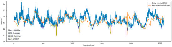
Figure 10.
Comparison between the SWH estimation of PWP-in at the buoy location and buoy-observed SWH in the time periods August 2018 and July 2019–September 2019.
4.3. Testing PWPNet
There is only one buoy in the port (ADCP1 in Figure 1), and observation periods are August 2018 and July 2019–September 2019. Due to limits in space and time, comparison with the buoy-observed SWH only cannot provide comprehensive test results for PWPNet.
Since PWP-in has good SSIM and PSNR compared to SWASH outputs, and fits with buoy-observed SWH well, we devised an alternative method shown in Figure 11 to test the performance of PWPNet and other 2-stage models for a whole year of 2020, where PWP-in was used to generate in-port SWH distribution in images as ground-truth. We tested PWPNet on these three time spans (25–48, 49–72, and 73–96 h) where PWP-out outperformed other methods, and compared it with other 2-stage models (LSTM, GRU, BPNN, SVR, ELM, and RF cascaded with PWP-in), namely LSTM+, GRU+, BPNN+, SVR+, ELM+, and RF+, and the evaluation metrics are SSIM and PSNR. The results shown in Figure 12 also suggest that PWPNet outperforms all other 2-stage cascaded models.
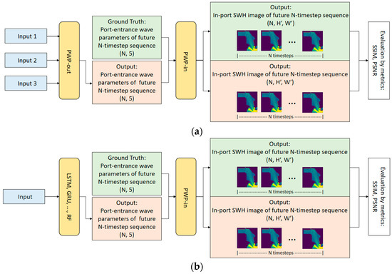
Figure 11.
A schematic diagram of testing PWPNet (a) and other 2-stage models (b).
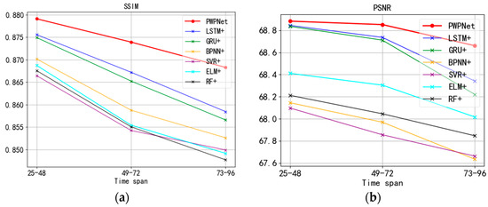
Figure 12.
Comparison of PWPNet with other cascaded models, metrics are SSIM (a) and PSNR (b).
The tests were carried out on a computer with the i3-7100 CPU and 16GB RAM, and the average time cost of a prediction using PWPNet is 0.0369 s, so it achieves real-time SWH prediction in a port.
5. Discussion
5.1. Discussion about the Performance of the Proposed Framework
Although the prediction accuracy of PWP-out is generally better than other models for medium-term (25–48 h), med–long-term (49–72 h), and long-term (73–96 h) predictions, the prediction accuracy of SWH in short-term prediction is still inferior to those models. Combining LSTM, GRU, BPNN, ELM, and RF with PWP-in for short-term prediction (1–24 h) can obtain better results. Moreover, some wave-prediction methods implemented empirical mode decomposition (EMD) as a preprocess of the original wave parameter sequences. We will attempt to improve short-term prediction results by integrating EMD as a part of our framework.
PWP-in, based on ANN, can estimate in-port SWH with good SSIM and PSNR, but it remains to be further improved. The Generative Adversarial Network (GAN) is another methodology adopted in a variety of applications including image synthesis [31]. In the future, we will attempt to improve in-port SWH estimation using GANs.
PWPNet utilizes outside-port 2D wave and wind field for prediction and does not rely on buoys in the port. The 2-stage error accumulation affects the prediction accuracy. In the future, we will utilize SWH data observed from ADCP1 [17] as an additional input to improve the performance of PWPNet.
Port-entrance wave parameters are greatly influenced by outside-port wind fields. Currently, PWPNet utilizes outside-port wind field data of historical timesteps, but there is room for further improvement, by utilizing outside-port wind field data of future timesteps. In the future, we will utilize outside-port wind field data forecasted by the atmospheric model of European Centre for Medium-Range Weather Forecasts (ECMWF) to improve the performance of PWPNet.
5.2. Discussion about the Data Availability
For port-entrance wave parameter prediction (PWP-out), the outside-port 2D wave and wind field data are downloaded from the ERA5 hourly reanalysis dataset on single levels [18] from the European Centre for Medium-Range Weather Forecasts (ECWMF). This dataset provides hourly estimations for a large number of atmospheric, ocean-wave and land–surface quantities, and is updated daily with a latency of about 5 days, so it cannot be directly used for real-time prediction. The ERA5 dataset is only for training and testing of PWP-out. When prediction is carried out, PWP-out can be combined with a numerical model providing wave field data of historical timesteps. As mentioned in Section 5.1, PWP-out will also be combined with an atmospheric model providing wind field data of future timesteps.
6. Conclusions
In this paper, a 2-stage deep learning framework (PWPNet) was proposed for real-time prediction of in-port SWH distribution. At the first stage, PWP-out predicts port-entrance wave parameters based on a novel 3-branch model, including the LSTM module for capturing the temporal dependencies of time sequences of port-entrance wave parameters, the Wave and Wind field Feature Extraction (WWFE) module composed of a residual network with spatial and channel attention for capturing spatiotemporal characteristics of outside-port 2D wave and wind field data, and a multi-scale time encoding for capturing the periodicity of waves and wind. At the second stage, PWP-in uses a customized ANN model to learn the nonlinear correlation between port-entrance wave parameters and in-port SWH to estimate the in-port SWH distribution. Comparison experiments showed that PWP-out outperformed mainstream machine learning methods, including LSTM, GRU, BPNN, SVR, ELM, and RF, in medium-term (25–48 h), med–long-term (49–72 h), and long-term (73–96 h) predictions of port-entrance wave parameters. Additionally, PWPNet outperformed other 2-stage models of LSTM, GRU, BPNN, SVR, ELM, and RF cascaded with PWP-in in the medium-term, med–long-term, and long-term predictions of in-port SWH distribution.
Author Contributions
Conceptualization, C.X. and X.L.; methodology, C.X.; software, X.L.; validation, C.X. and X.L.; investigation, Y.Z. and T.M.; data curation, X.M., G.D., T.M., T.X. and X.L.; writing—original draft preparation, X.L.; writing—review and editing, C.X. and J.D.; visualization, C.X., X.L. and T.X.; supervision, C.X. and J.D.; project administration, Y.Z. and C.X. All authors have read and agreed to the published version of the manuscript.
Funding
This research was funded by the National Key Research and Development Program of China, grant number 2020YFE0201200 and 2019YFC1509100; the National Natural Science Foundation of China (NSFC), grant number 41706010, U1706218, and 41927805; the Fundamental Research Funds for the Central Universities, grant number 202264002.
Institutional Review Board Statement
Not applicable.
Informed Consent Statement
Not applicable.
Data Availability Statement
Not applicable.
Conflicts of Interest
The authors declare no conflict of interest.
References
- Dong, G.; Zheng, Z.; Ma, X.; Huang, X. Characteristics of low-frequency oscillations in the Hambantota Port during the southwest monsoon. Ocean. Eng. 2020, 208, 107408. [Google Scholar] [CrossRef]
- Wang, G.; Stanis ZE, G.; Fu, D.; Zheng, J.; Gao, J. An analytical investigation of oscillations within a circular harbor over a Conical Island. Ocean. Eng. 2020, 195, 106711. [Google Scholar] [CrossRef]
- The Wamdi Group. The WAM model—A third generation ocean wave prediction model. J. Phys. Oceanogr. 1988, 18, 1775–1810. [Google Scholar] [CrossRef]
- Tolman, H.L. User Manual and System Documentation of WAVEWATCH III TM Version 3.14; Technical Note, MMAB Contribution; U.S. Department of Commerce, National Oceanic and Atmospheric Administration, National Weather Service, National Centers for Environmental Prediction: Camp Springs, MD, USA, 2009; pp. 1–220.
- Booij, N.; Holthuijsen, L.H.; Ris, R.C. The “SWAN” wave model for shallow water. Coast. Eng. 1996, 1, 668–676. [Google Scholar]
- Zijlema, M.; Stelling, G.; Smit, P. SWASH: An operational public domain code for simulating wave field and rapidly varied flows in coastal waters. Coast. Eng. 2011, 58, 992–1012. [Google Scholar] [CrossRef]
- Chen, Q. Fully nonlinear Boussinesq-type equations for waves and currents over porous beds. J. Eng. Mech. 2006, 132, 220–230. [Google Scholar] [CrossRef]
- Wornom, S.F.; Welsh DJ, S.; Bedford, K.W. On coupling the SWAN and WAM wave models for accurate nearshore wave predictions. Coast. Eng. J. 2001, 43, 161–201. [Google Scholar] [CrossRef]
- Choi, Y.K.; Seo, S.N.; Choi, J.Y.; Shi, F.; Park, K.-S. Wave prediction in a port using a fully nonlinear Boussinesq wave model. Acta Oceanol. Sin. 2019, 38, 36–47. [Google Scholar] [CrossRef]
- Ali, M.; Prasad, R. Significant wave height forecasting via an extreme learning machine model integrated with improved complete ensemble empirical mode decomposition. Renew. Sustain. Energy Rev. 2019, 104, 281–295. [Google Scholar] [CrossRef]
- Kumar, N.K.; Savitha, R.; Al Mamun, A. Ocean wave characteristics prediction and its load estimation on marine structures: A transfer learning approach. Mar. Struct. 2018, 61, 202–219. [Google Scholar] [CrossRef]
- Law, Y.Z.; Santo, H.; Lim, K.Y.; Chan, E.S. Deterministic wave prediction for unidirectional sea-states in real-time using Artificial Neural Network. Ocean. Eng. 2020, 195, 106722. [Google Scholar] [CrossRef]
- Demetriou, D.; Michailides, C.; Papanastasiou, G.; Onoufriou, T. Coastal zone significant wave height prediction by supervised machine learning classification algorithms. Ocean. Eng. 2021, 221, 108592. [Google Scholar] [CrossRef]
- Fan, S.; Xiao, N.; Dong, S. A novel model to predict significant wave height based on long short-term memory network. Ocean. Eng. 2020, 205, 107298. [Google Scholar] [CrossRef]
- Wang, J.; Wang, Y.; Yang, J. Forecasting of significant wave height based on gated recurrent unit network in the taiwan strait and its adjacent waters. Water 2021, 13, 86. [Google Scholar] [CrossRef]
- Gopinath, D.I.; Dwarakish, G.S. Wave prediction using neural networks at New Mangalore Port along west coast of India. Aquat. Procedia 2015, 4, 143–150. [Google Scholar] [CrossRef]
- Zheng, Z.; Ma, X.; Ma, Y.; Dong, G. Wave estimation within a port using a fully nonlinear Boussinesq wave model and artificial neural networks. Ocean. Eng. 2020, 216, 108073. [Google Scholar] [CrossRef]
- Hersbach, H.; Bell, B.; Berrisford, P.; Hirahara, S.; Horányi, A.; Muñoz-Sabater, J.; Nicolas, J.; Peubey, C.; Radu, R.; Schepers, D.; et al. The ERA5 global reanalysis. Q. J. R. Meteorol. Soc. 2020, 146, 1999–2049. [Google Scholar] [CrossRef]
- Hashim, R.; Roy, C.; Motamedi, S.; Shamshirband, S.; Petković, D. Selection of climatic parameters affecting wave height prediction using an enhanced Takagi-Sugeno-based fuzzy methodology. Renew. Sustain. Energy Rev. 2016, 60, 246–257. [Google Scholar] [CrossRef]
- Blayo, E.; Debreu, L. Revisiting open boundary conditions from the point of view of characteristic variables. Ocean. Model. 2005, 9, 231–252. [Google Scholar] [CrossRef]
- Hasselmann, K.; Barnett, T.P.; Bouws, E.; Carlson, H.; Cartwright, D.E.; Enke, K.; Ewing, J.A.; Gienapp, H.; Hasselmann, D.E.; Kruseman, P.; et al. Measurements of Wind-Wave Growth and Swell Decay during the Joint North Sea Wave Project (JONSWAP); Deutsches Hydrographisches Institut: Hamburg, Germany, 1973. [Google Scholar]
- Suzuki, T.; Altomare, C.; Veale, W.; Verwaest, T.; Trouw, K.; Troch, P.; Zijlema, M. Efficient and robust wave overtopping estimation for impermeable coastal structures in shallow foreshores using SWASH. Coast. Eng. 2017, 122, 108–123. [Google Scholar] [CrossRef]
- Battjes, J.A.; Janssen, J. Energy loss and set-up due to breaking of random waves. Coast. Eng. Proc. 1978, 1, 32. [Google Scholar] [CrossRef]
- Smit, P.; Zijlema, M.; Stelling, G. Depth-induced wave breaking in a non-hydrostatic, near-shore wave model. Coast. Eng. 2013, 76, 1–16. [Google Scholar] [CrossRef]
- Van Leer, B. Towards the ultimate conservative difference scheme. V. A second-order sequel to Godunov’s method. J. Comput. Phys. 1979, 32, 101–136. [Google Scholar] [CrossRef]
- De Moura, C.A.; Kubrusly, C.S. The Courant–Friedrichs–Lewy (CFL) Condition; Birkhäuser: Boston, MA, USA, 2013; pp. 53–61. [Google Scholar]
- Hochreiter, S.; Schmidhuber, J. Long short-term memory. Neural Comput. 1997, 9, 1735–1780. [Google Scholar] [CrossRef]
- He, K.; Zhang, X.; Ren, S.; Sun, J. Deep residual learning for image recognition. In Proceedings of the 2016 IEEE Conference on Computer Vision and Pattern Recognition (CVPR), Las Vegas, NV, USA, 27–30 June 2016; pp. 770–778. [Google Scholar]
- Jayawardena IM, S.P.; Punyawardena, B.V.R.; Karunarathne, M. Importance of integration of subseasonal predictions to improve climate services in Sri Lanka case study: Southwest monsoon 2019. Clim. Serv. 2022, 26, 100296. [Google Scholar] [CrossRef]
- Shao, J. Linear model selection by cross-validation. J. Am. Stat. Assoc. 1993, 88, 486–494. [Google Scholar] [CrossRef]
- Creswell, A.; White, T.; Dumoulin, V.; Arulkumaran, K.; Sengupta, B.; Bharath, A.A. Generative adversarial networks: An overview. IEEE Signal Process. Mag. 2018, 35, 53–65. [Google Scholar] [CrossRef]
Publisher’s Note: MDPI stays neutral with regard to jurisdictional claims in published maps and institutional affiliations. |
© 2022 by the authors. Licensee MDPI, Basel, Switzerland. This article is an open access article distributed under the terms and conditions of the Creative Commons Attribution (CC BY) license (https://creativecommons.org/licenses/by/4.0/).