On the Sparse Gradient Denoising Optimization of Neural Network Models for Rolling Bearing Fault Diagnosis Illustrated by a Ship Propulsion System

Abstract

The drive rolling bearing is an important part of a ship’s system; the detection of the drive rolling bearing is an important component in ship-fault diagnosis, and machine learning methods are now widely used in the fault diagnosis of rolling bearings. However, training methods based on small batches have a disadvantage in that the samples which best represent the gradient descent direction can be disturbed by either other samples in the opposite direction or anomalies. Aiming at this problem, a sparse denoising gradient descent (SDGD) optimization algorithm, based on the impact values of network nodes, was proposed to improve the updating method of the batch gradient. First, the network is made sparse by using the node weight method based on the mean impact value. Second, the batch gradients are clustered via a distribution-density-based clustering method. Finally, the network parameters are updated using the gradient values after clustering. The experimental results show the efficiency and feasibility of the proposed method. The SDGD model can achieve up to a 2.35% improvement in diagnostic accuracy compared to the traditional network diagnosis model. The training convergence speed of the SDGD model improves by 2.16%, up to 17.68%. The SDGD model can effectively solve the problem of falling into the local optimum point while training a network.

1. Introduction

With the rapid development of the global economy, maritime transportation logistics have become an important lifeline to the global economy. The safe and reliable operation of the power transmission equipment of large marine ships is critical to the marine logistic enterprise. In order to meet the needs of production, marine powertrain equipment usually needs to work for a long time or even under a state of overload, which leads to the most common failure of the rolling bearing system in the powertrain [1]. Once these failures occur, they can cause huge economic losses. These accidents make people realize the importance of fault diagnosis in marine powertrain equipment. If the faults can be found and repaired in time, according to the operation data of the equipment, the loss can be effectively retrieved [2].

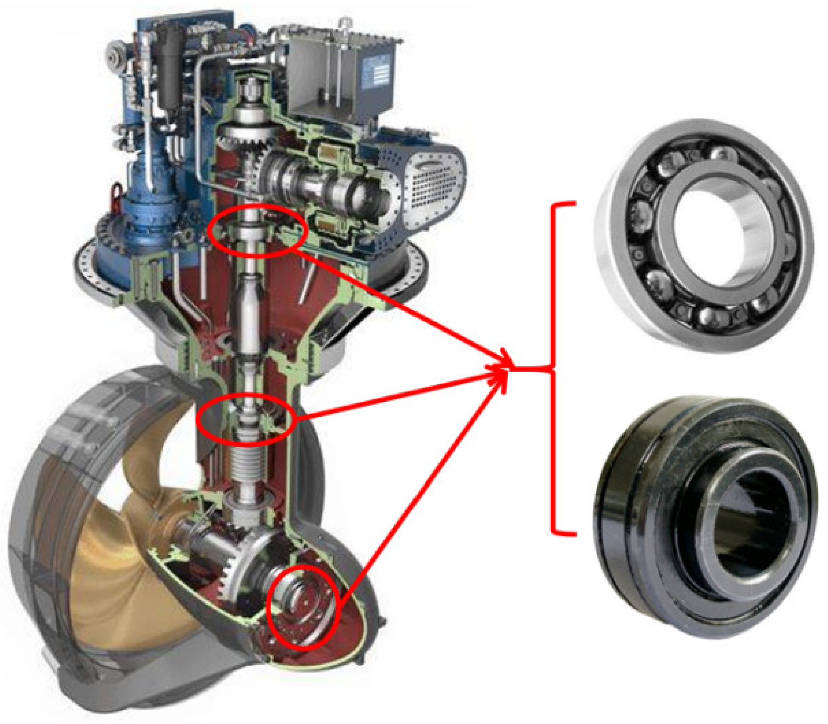
As shown in Figure 1, the internal power and transmission system inside a ship includes the engine and a large number of rotational parts, most of which include rolling bearings, and the frictional wear of these bearings occurs continuously with mechanical movement. These bearing faults account for a considerable proportion of all powertrain failures [3].

Model-based diagnosis methods are the most commonly used in the field of fault diagnosis [4]. By analyzing the operation process of the equipment, a fault diagnosis model is established for performing effective fault diagnosis. However, the wear and aging of rolling bearings often have a non-linear or uncertain correspondence and are always accompanied by the failure of other components. Multiple faults may occur simultaneously and interact with each other, so it is difficult to build the fault diagnosis model accurately [5].

Data-driven fault diagnosis methods can effectively demonstrate the operation information and the fault status from a large amount of historical data [6]. Based on the obtained historical data, a data-driven diagnosis model can be built to provide an effective diagnosis result [7]. Commonly used data-driven fault diagnosis methods include the artificial neural network (ANN) algorithm [8], autoencoder [9], and Bayesian network [10].

Feature extraction is an important step for data-driven fault diagnosis based on neural networks. Frequency domain feature extraction is the most commonly used method [11]. Hu et al. [12] applied kernel principal component analysis (KPCA) and wavelet packet decomposition methods to extract features from continuous, raw time signals and feed the features to a weighted limit learning machine for classification and diagnosis. A feature extraction approach based on the sparse filtering of the raw data was proposed in [13]. However, some diagnosis networks can extract data features themselves. The convolutional operation is the most commonly used method to extract data features [14,15]. In order to make the diagnosis network more adaptable to multiple fault types, Cai et al. [16] investigated deep Bayesian networks to model the dynamic processes of faults, as well as Markov chains for different fault types, including transient faults, intermittent faults, and permanent faults. The network-based methods have some disadvantages. During the training process of diagnosis networks, they often fall into local optimal points. Tao et al. [17] addressed the fact that adding a genetic element to the updating process of the gradients can improve the convergence speed effectively as well as the accuracy of the diagnosis network.

There are numerous research results on how to alleviate diagnosis networks from falling into local optimal points and improve the convergence speed. Stochastic gradient descent (SGD) was first applied to solve the problem, where one sample is randomly selected in each training epoch to represent the updated gradient values of all samples. The SGD method is sensitive to gradient noise and tends to fall into local optimal points [18]. Then, full-batch gradient descent (FGD) was proposed, where the gradients of all samples are obtained during each training epoch, and then take the mean value as the updating gradient. The FGD method is highly undesirable due to the iteration efficiency being too low when the sample size is huge [19]. The mini-batch gradient descent (MGD) method combines the advantages of both SGD and FGD [20]. The number of samples taken during each iteration is fixed, and the mean value of these sample gradients is used as the updating value. This method is currently the most widely used one [21].

In order to achieve faster convergence speeds for the network during the training process, a series of improvements have been made based on stochastic gradient descent algorithms. By adding a momentum factor, the historic gradient changing information can be integrated to improve the optimization efficiency [22]. The momentum updating strategies include the classical momentum algorithm (CM) and the Nesterov accelerated gradient algorithm (NAG) [23,24]. In order to reduce the continuous accumulation of the gradient variance during random sampling in the iterative process, researchers have proposed the stochastic variance reduction gradient algorithm (SVRG), which gives a general framework for variance reduction algorithms [25]. The subsequent variance reduction algorithms that emerged successively, mostly improved upon this version, such as VR-SGD and stochastic primal-dual coordinates (SPDC) [26,27]. The accelerated gradient methods reserve a corresponding gradient value for each sample. During the iteration process, samples are drawn in turn and replaced the former gradients with new ones [28]. The stochastic average gradient algorithm (SAG), augmented Lagrange-stochastic gradient algorithm (AL-SGA), and point-SAGA were derived based on different updating strategies [29,30,31]. The adaptive learning rate adjustment algorithm allows for the flexible online adjustment of the learning rate. It can reduce oscillations and speed up convergence during the training process. According to the different adjustment strategies, some scholars proposed the adaptive gradient (Adagrad) [32] and adaptive moment estimation (Adam) [33] algorithms for the adaptive adjustment of learning rate.

However, it has been pointed out that large-scale training datasets have the problem of sample redundancy [34]. The noise and imbalanced distribution of sample gradients are not fully considered. Somehow, falling into a local optimal point is still a serious issue.

Based on the above analysis, a new sparse denoising gradient descent (SDGD) network model was proposed to improve the updating method of the batch gradient. The algorithm proposed in this paper can obviously improve the convergence speed of the neural network and effectively solve the problem of falling into local optimal points during network model training.

The main contributions of the work can be summarized as follows.

(1) A sparse method based on mean impact values is proposed. The network nodes are weighted based on the mean impact value sparse method, and then the key nodes of the network are marked. The network parameters can be effectively “sparsed”.

(2) The density-based spatial clustering of applications with noise (DBSCAN) method was used to cluster and denoise the batch gradients. The parameters after denoising can obviously improve the convergence speed of the training and effectively solve the problem of falling into local optimal points.

The rest of this paper is organized as follows. Section 2 provides the preliminaries. Section 3 gives a specific description of the proposed SDGD optimization algorithm. Section 4 gives a case study. Section 5 draws a conclusion and presents the future work.

2. Preliminaries

2.1. Fault Diagnosis of Marine Machinery

For modern maritime ships, effective machinery fault diagnosis is essential [35]. The existing data-driven intelligent recognition methods that are widely used mainly collect historical data through a large number of sensors to establish an intelligent recognition model, so that it has effective recognition ability. Yan et al. performed fault diagnosis by means of vibration signals collected from marine blowers [36]. Firstly, the time domain vibration signal was extracted by the EEMD method, and then the diagnostic model was constructed by the back propagation neural network (BPNN). The EEMD-BPNN intelligent diagnostic method has excellent diagnostic results for marine blowers. Xu et al. [37] combined expert knowledge and data-driven methods effectively. The model was first set up by an expert system and then optimized using historical data. Thus, a belief, rule-based expert system for the fault diagnosis of marine diesel engines was established. Xu et al. [38] proposed an approach that fused multiple data-driven models for the fault diagnosis of a marine diesel engine. The method can effectively fuse the predictions of individual models, and the results are often more reliable than single data-driven diagnosis models. Tan et al. [39] proposed a one-class SVM-based approach for the diagnosis of the main propulsion system in a ship’s operation. Compared with traditional methods, this method can effectively reduce the amount of data required. A model based on neural networks was developed to detect the state of ship engine systems [40]. Operational data from the machine were first collected, and then the diagnostic network was trained. The diagnostic modeling of long- and short-term memory (LSTM) networks, combined with automatic encoders, has also been used more often in the diagnosis of marine machinery [41,42]. LSTM has an advantage with time-series input signals.

Compared with other data-based fault diagnosis methods in the industry, the diagnostic approach for maritime ships is generally consistent. First, the historical data signals are collected via sensors. Then, feature extraction of the signal is performed. Finally, the model of the diagnosis network is established [43,44]. However, these approaches are essentially rudimentary applications of neural networks and fail to consider some practical problems in the data-training efficiency of maritime ship environments. How to increase the speed of training convergence efficiency, effectively improving the diagnosis accuracy, and avoid falling into local optimum points during the training process needs to be addressed urgently.

2.2. Overview of the Density-Based Spatial Clustering of Applications with Noise (DBSCAN)

Density-based spatial clustering of applications with noise (DBSCAN) is a density-based clustering algorithm. The three important definitions in DBSCAN: density reachable, and density connection, are shown in Figure 2.

Assume a sample set, $D=(d_1,d_2,\dots ,d_B)$, where B is the number of the samples. The DBSCAN algorithm is executed as follows: First, the neighborhood, $\zeta$, and the minimum number of density points, MinPts, are set. Second, select a random point, $d_i$, from the sample set. Next, determine whether $d_i$ is a core object. If the data $d_i$ is a core object, all “density reachable” points of $d_i$ in the sample data set are found and a new bunch with all other density reachable points is created. Third, a cluster is obtained based on the “density connected” of all points in the bunch. Following the above steps, all the data points in the sample data set are processed to obtain the final clustering result: $D^{\prime }=({d^{\prime }}_1,{d^{\prime }}_2,\dots ,{d^{\prime }}_{B^{\prime }})$, as well as the noise. The above clustering process is noted as Equation (1).

$$({d^{\prime }}_i|i=1,2\dots B^{\prime })=f_d\left(d_i|i=1,2\dots B\right),B^{\prime }\le B$$

(1)

3. The Proposed SDGD Model

We propose an optimization method to select valuable nodes based on the mean impact value of the nodes in the network. The gradients of the valuable nodes were clustered and denoised using the DBSCAN method. Considering the information of each sample’s updating gradient inside a batch as a vector, it is assumed that they obey a certain distribution. In this way, we conduct clustering on this gradient information and remove the noisy gradients, which can effectively avoid the drawbacks of the original method of averaging by simply summation.

3.1. Keys Nodes Sparse Method Based on Mean Impact Value

Studies related to network sparsity have shown that only few of the nodes in a multi-layer multi-node network have a critical impact on the propagation of the subsequent layers. The mean impact value (MIV) method can quantify the impact weight of each neural node in the network propagation. For a neural network, the sample dataset is $X=(X_1,X_2,\dots ,X_N)$, where $X_n^{}=(x_n^1,x_n^2,\dots ,x_n^l,\dots ,x_n^{L_1})$. The $h\mathrm{th}$ layer of the network has $L_h$ nodes. The input of the $h\mathrm{th}$ layer corresponding to the input of $X_n^{}$ is $U_n^h=(u_n^1,u_n^2,\dots ,u_n^l,\dots ,u_n^{L_h})$, and the output of the layer is $V_n^h=(v_n^1,v_n^2,\dots ,v_n^l,\dots ,v_n^{L_h})$. The key nodes sparse method based on MIV is described as follows.

At the $h\mathrm{th}$ layer, the self-increment and self-subtraction operation is carried out on the input of its $l\mathrm{th}$ node.

$$U_{n,\pm \delta }^{h_l}=(u_n^1,u_n^2,\dots ,(1\pm \delta )u_n^l,\dots ,u_n^{L_h})$$

(2)

where, $U_{n,\pm \delta }^{h_l}$ is propagated from the $h\mathrm{th}$ layer to the output layer. The nonlinear iterative process transmitted forward from the $h\mathrm{th}$ layer is denoted as $\widehat{Y}=F_h(U^h)$, where ${\psi }_h$ is the nonlinear activation function of the $h\mathrm{th}$ layer. The new output obtained is noted as

$$\begin{array}{ll}{\widehat{Y}}_{\pm }^{h_l}& ={\displaystyle \sum _{j=h}^H{\psi }_j[{\omega }_j{U}_{n,\pm \delta }^{h_l}+b_j]}\\ & ={\displaystyle \sum _{j=h}^H{\psi }_j[{\displaystyle \sum _{i=1}^{L_j}{\omega }_{ij}{u}_{n,\pm \delta }^i}+b_{ij}]}\\ & =F_h(U_{n,\pm \delta }^{h_l})\end{array}$$

(3)

Therefore,

$$\begin{array}{ll}I{V}_l^h& ={\Vert {\widehat{Y}}_{+}^{h_l}-{\widehat{Y}}_{-}^{h_l}\Vert }_1\\ & ={\Vert {\displaystyle \sum _{j=h}^H{\psi }_j[{\displaystyle \sum _{i=1}^{L_j}{\omega }_{ij}{u}_{n,+\delta }^i}+b_{ij}]}-{\displaystyle \sum _{j=h}^H{\psi }_j[{\displaystyle \sum _{i=1}^{L_j}{\omega }_{ij}{u}_{n,-\delta }^i}+b_{ij}]}\Vert }_1\\ & =\Vert F_h(U_{n,+\delta }^{h_l}){-F_h(U_{n,-\delta }^{h_l})\Vert }_1\end{array}$$

(4)

where $I{V}_l^h$ is the impact value of the $l\mathrm{th}$ neuron in $h\mathrm{th}$ layer for the diagnosis network output. Similarly, the impact values of all other neurons in the $h\mathrm{th}$ layer can be derived as Equation (5).

$$I{V}^h=[I{V}_1^h,I{V}_2^h,\dots ,I{V}_l^h,\dots ,I{V}_{L_h}^h]$$

(5)

Each element in $I{V}^h$ is the impact value of the corresponding neuron in the $h\mathrm{th}$ layer of the output. $MI{V}^h$ can be obtained by summing up all the elements together.

$$MI{V}^h=\frac{1}{L_h}{\displaystyle \sum _{i=1}^{L_h}I{V}_i^h}$$

(6)

The value obtained by dividing $I{V}_l^h$ with $MI{V}^h$ can be considered as the relative impact value of the corresponding node. Based on the obtained relative impact values, the nodes in this layer can be effectively sparsed. Before the batch internal gradients update, the impact value threshold of the node can be set to $\theta$. The nodes in each layer are filtered according to $\theta$. If the impact value of the corresponding node is greater than $\theta$, the node is marked as a key node, otherwise this node is sparsed. The connection values between key nodes are updated using DBSCAN. The remaining connection values are obtained by BSGD. By this method, the complexity of the algorithm operations is greatly reduced while the gradient updating is effectively performed.

3.2. Clustering Noise Reduction Method Based on Distribution Density

It is generally accepted that within each batch, the distribution density of its superior gradients will be greater than the distribution density of the other noisy updating values. The values outside the distribution edge of the intra-batch gradient clustering are treated as noise. In the process of training the diagnosis network, the loss function of the network is defined as Equation (7). B is the sample size of the batch.

$$\begin{array}{ll}{J}_b|b=1,2\dots B& =\frac{1}{2}{\displaystyle \sum _{l=1}^{L_H}{e}_l^2+\lambda {{\displaystyle \sum (\omega )}}^2}\\ & =\frac{1}{2}{\displaystyle \sum _{l=1}^{L_H}{(y_l-{\widehat{y}}_l)}^2}+\lambda {{\displaystyle \sum (\omega )}}^2\end{array}$$

(7)

where ${{\displaystyle \sum (\omega )}}^2$ denotes the $L_2$-normalization of all parameters of the network, and $\lambda$ is the weight coefficient of the normalization term. The updating formulas for the weights $\nabla {\omega }_{ij}^b$ based on DBSCAN are as follows.

$$\nabla {{\omega }^{\prime }}_{ij}^{}=\frac{1}{B^{\prime }}{\displaystyle \sum _{n=1}^{B^{\prime }}{d^{\prime }}_n}$$

(8)

$$({d^{\prime }}_n|n=1,2\dots B^{\prime })=f_d\left(d_n|n=1,2\dots B\right)$$

(9)

$$\begin{array}{ll}{d}_n& =\frac{\partial J_n}{\partial {\omega }_{ij}}|n=1,2\dots B\\ & =\frac{\partial \left(\frac{1}{2}{[{\displaystyle \sum _{j=1}^H{\psi }_j({\displaystyle \sum _{i=1}^{L_j}{\omega }_{ij}{x}_n^i}+b_{ij})}-y_n]}^2+\lambda {\displaystyle \sum _{j=1}^H{\displaystyle \sum _{i=1}^{L_j}{[{\omega }_{ij}]}^2}}\right)}{\partial {\omega }_{ij}}\end{array}$$

(10)

The updating process of $\nabla {b^{\prime }}_{ij}^{}$ based on DBSCAN is similar and will not be detailed here.

3.3. Sparse Denoising Gradient Descent Optimization Algorithm

This section will introduce the sparse gradient denoising optimization algorithm in detail. Compared with the original algorithm’s strategy of summing up the gradients in the batch and averaging them, this algorithm denoises the gradients of the samples within the batch using the DBSCAN-clustering method and then updating the gradients.

The structure diagram of the algorithm is shown in Figure 3. The key nodes of the network are marked by the MIV-sparse algorithm during each iteration, and the connection weights between the key nodes are clustered and denoised by the DBSCAN algorithm. Then the network weights are updated until the network training stopping condition is satisfied. The trained diagnosis network is used to diagnose the test data and gives the diagnosis results.

The training flow for the sparse denoising gradient decent optimization algorithm is shown in Figure 4.

The process of the sparse denoising gradient descent optimization algorithm is described as follows.

(1) Setting network parameters: $[L_1,L_2,\dots ,L_H]$. BatchSize = B, learning rate $\eta$, impact value threshold $\theta$, and the network connection parameters are randomly initialized. The training loss stop condition threshold $J_0$ and training epochs are set;

(2) The samples in the batch are sequentially fed into the network for forward propagation to obtain the predicted output value corresponding to that sample, and $J_b$ is calculated. According to the loss $J_b$, the backward derivative is derived and the gradient updated values $\nabla {\omega }_{ij}^b=\frac{\partial J_b}{\partial {\omega }_{ij}}$, $\nabla b_{ij}^b=\frac{\partial J_b}{\partial b_{ij}}$ of all nodes of the network corresponding to each sample are calculated.

(3) According to Algorithm 1, all nodes of the network are marked and $Net\_Lab$ is obtained. Gradients of connection weights between key nodes are updated using the DBSCAN method $\nabla {{\omega }^{\prime }}_{ij}^{}=f_d(\nabla {\omega }_{ij}^b|b=1,2\dots B)$, $\nabla {b^{\prime }}_{ij}^{}=f_d(\nabla b_{ij}^b|b=1,2\dots B)$. The results are obtained by summing up and taking the average. ${\omega }_{ij}(k+1)={\omega }_{ij}(k)-\eta \cdot \nabla {{\omega }^{\prime }}_{ij}^{}$, $b_{ij}(k+1)=b_{ij}(k)-\eta \cdot \nabla {b^{\prime }}_{ij}^{}$

Algorithm 1: MIV-Sparse algorithm.

-B: batch size; -H: number of network layers; -$[L_1,L_2,\dots ,L_H]$: node numbers per network layer; -$U_{}^h$: input of the $h\mathrm{th}$ layer; -$\widehat{Y}=F_h(U^h)$: the nonlinear iterative process transmitted from the $h\mathrm{th}$ layer backward; -Input: network: $[L_1,L_2,\dots ,L_H]$, impact value threshold $\theta$, training dataset -Output: spared network: $Net\_Lab$ 1.  for n = 1…B do              //samples traversal 2.  for i = 1…H do               //transmission between input and output layers 3.    for k = 1…$L_i$ do              //node traversal per layer 4.      $U_{n,\pm \delta k}^{h_i}=(u_n^1,u_n^2,\dots ,(1\pm \delta )u_n^k,\dots ,u_n^{L_i})$  //self-increment and self-subtraction operation 5.      Forward Propagation: ${\widehat{Y}}_{n,\pm k}^{h_i}=F_i(U_{n,\pm \delta k}^{h_i})$ 6.      $I{V}_{n,k}^{h_i}={\Vert {\widehat{Y}}_{n,+k}^{h_i}-{\widehat{Y}}_{n,-k}^{h_i}\Vert }_1=\Vert F_i(U_{n,+\delta k}^{h_i}){-F_i(U_{n,-\delta k}^{h_i})\Vert }_1$ 7.    end for                  //quit node traversal 8.  $I{V}_n^{h_i}=[I{V}_{n,1}^{h_i},I{V}_{n,2}^{h_i},\dots ,I{V}_{n,k}^{h_i},\dots ,I{V}_{n,L_i}^{h_i}]$      //impact value vector of the $i\mathrm{th}$ layer 9.  Summation comparison: $I{V}_n^{h_i}=I{V}_n^{h_i}/\frac{1}{L_i}{\displaystyle \sum _{k=1}^{L_i}I{V}_{n,k}^{h_i}}$ 10.  end for                  //quit layer traversal 11. end for                  //quit samples traversal 12. for i = 1…H do                //marked the key nodes 13.  $I{V}_{}^{h_i}=\frac{1}{B}{\displaystyle \sum _{n=1}^{B}I{V}_n^{h_i}}$ 14.  All elements within $I{V}_{}^{h_i}$ are compared with $\theta$. The network node greater than $\theta$ is marked as 1, otherwise it is marked as 0, and spare network $Net\_Lab$ is obtained. 15. end for

The Pseudo code and flow chart of SDGD algorithm are shown in Algorithm 2 and Figure 5, respectively. During the forward propagation of the network, the key nodes of the net are marked with the MIV-sparse method. According to the loss function, $J_b$ of each sample is calculated. Finally, gradients of the connection weights between the key nodes are updated using the DBSCAN method.

Algorithm 2: Sparse denoising gradient decent optimization algorithm

-$J_b$: loss function; -$\nabla \omega$: connection weight gradient; -$\nabla b$: connection bias gradient; -$IV$: impact value of nodes; -$MIV$: mean impact value; -Input: network parameters $[L_1,L_2,\dots ,L_H]$, BatchSize = B, learning rate $\eta$, impact value threshold $\theta$, training loss stop condition threshold $J_0$, training epochs; -Output: the trained network $Ne{t}_{tra}$ 1. for  k = 1…epochs  do        //Cycle epochs times 2.  for b = 1…B do        //All samples traversal 3.    Calculating $\widehat{Y}=F_1(X_b)$            //Forward propagation 4.    Calculating loss function $J_b$; 5.    if $J_b\le J_0$                //Whether the stopping condition is satisfied 6.        yes:stop training; 7.    else 8.      $\nabla {\omega }_{ij}^b=\frac{\partial J_b}{\partial {\omega }_{ij}}$, $\nabla b_{ij}^b=\frac{\partial J_b}{\partial b_{ij}}$;   //Calculate the corresponding gradient update value for each sample 9.      get $Net\_Lab$            //$Net\_Lab$ is obtained according to Algorithm 1 10.      $\nabla {{\omega }^{\prime }}_{ij}^{}=f_d(\nabla {\omega }_{ij}^b|b=1,2\dots B)$, $\nabla {b^{\prime }}_{ij}^{}=f_d(\nabla b_{ij}^b|b=1,2\dots B)$ //Calculating gradient update values by DBSCAN method; 11.      ${\omega }_{ij}(k+1)={\omega }_{ij}(k)-\eta \cdot \nabla {{\omega }^{\prime }}_{ij}^{}$, $b_{ij}(k+1)=b_{ij}(k)-\eta \cdot \nabla {b^{\prime }}_{ij}^{}$ //Updating network connection weights 12.    end if 13.  end for 14. end for

The input data for each batch in Figure 5 are $X_1,X_2,\dots ,X_B$ and $X_1^{}=(x_1,x_2,\dots ,x_l,\dots ,x_{L1})$. The network consists of three pieces: the input layer, the hidden layers, and the output layer. The white neurons in the network layer indicate less important nodes after MIV filtering. The black neurons indicate key nodes. The neuronal connections between all key nodes are indicated by the purple connecting lines, which are updated with the SDGD algorithm during the gradient update. The rest of the connection lines are connected by dashed lines. The red arrows in the output layer indicate that the output value is positive at that location, while blue is negative. The input data are first propagated forward, indicated by the large green arrow, to give the predicted output $\widehat{Y}$. The loss value, $J$, is calculated after a comparison with the real output. The network weights are then updated by back-propagating through the large red arrow. $W\&B$ in the figure indicates the network weights. The network structure in Figure 5 is an abstract representation. For a convolutional-type network, the input and hidden layers correspond to the convolutional and pooling layers. While the output layer corresponds to the flattened and fully connected layers as well as the output layer.

4. Validation Experiments

In order to demonstrate the effectiveness of the proposed method for fault diagnoses, two fault diagnosis experiments were conducted to verify it. The advantages of the proposed method are mainly reflected in its ability to improve the convergence rate of the existing algorithms in the training process, avoid local optimization, and prevent oversaturation. It represents an improvement in the training process. The existing data-driven intelligent diagnosis methods can be divided into two categories. One is the network model, with a strong feature extraction ability, such as convolutional neural networking and its deformation. The other is to process the signal first, extract the characteristics of the signal, and then send them to the network model, such as DNN and SVM. Therefore, in this part of the experimental verification, we selected several widely used network structures in the field of fault diagnosis: Resnet, random CNN, SAE, and DNN, based on feature extraction of the original data for comparative experimental analysis.

The diagnostic object of case one is a “motor drive system bearings dataset” publicly available at Case Western Reserve University. In this case, we use a fault diagnosis method based on Resnet random-CNN and -SAE. The experimental results show that the proposed algorithm in the manuscript has significantly improved the diagnostic accuracy and training convergence speed of the network. The object of case two is the rolling bearing dataset published by Xi’an Jiaotong University. In this case, a fault diagnosis neural network based on time-frequency domain feature extraction is built. The experimental results show that the proposed algorithm significantly improved the solving of the local optimal point trap.

4.1. Case One: Study of Accuracy & Convergence Speed of Fault Diagnosis Model

4.1.1. Dataset Preparation and Parameter Settings

This experiment case uses the open-source rolling bearing fault dataset from Case Western Reserve University as the experimental dataset [45]. The experimental object is a motor drive system. The vibration acceleration signal of the device is collected by installing sensors at different locations in the drive system. The collection location includes the drive end, fan end, and base. The load on the motor can change during operation. The load change range is 0–3 hp. The states of the bearing after failure are simulated by manually setting different levels of damage at various locations on the bearing. The details of the three different degrees and the three different locations of damage are shown in

Table 1. Data information for the nine types of fault states.

Fault Type	Fault Diameter (inch)	Label	Sample Size
BDⅠ	0.007	1	1000
BDⅡ	0.014	2	1000
BDⅢ	0.021	3	1000
IRⅠ	0.007	4	1000
IRⅡ	0.014	5	1000
IRⅢ	0.021	6	1000
ORⅠ	0.007	7	1000
ORⅡ	0.014	8	1000
ORⅢ	0.021	9	1000

. They combine with each other for a total of nine different faults. The data selected for this experiment were collected by drive end at a 0 hp load. They are ball defect Ⅰ (BDⅠ), ball defect Ⅱ (BDⅡ), ball defect Ⅲ (BD Ⅲ), inner race defect Ⅰ (IRⅠ), inner race defect Ⅱ (IRⅡ), inner race defect Ⅲ (IRⅢ), outer race defect Ⅰ (ORⅠ), outer race defect Ⅱ (ORⅡ), and outer race defect Ⅲ (ORⅢ), respectively. The sampling frequency of the vibration sensor was 12 kHz and the motor speed was set to 1772 rpm. It can be calculated that there are about 400 sampling points per circle. The sample status information is shown in Table 1. The samples are processed using a k-fold cross validation method in order to ensure that the experiment results are non-accidental.

The acceleration signals for the nine types of faults on the drive end are shown in Figure 6.

In the process of the experimental validation, after many experiments and analyses, we have given a range for the selection of the parameters. First, for the two parameters, $\zeta$ and MinPts, of DBSCAN, we know that, for the minimum distance, $\zeta$, if the value is set too large, the denoising effect will not be achieved; if it is too small, the total number of categories will be too large. Therefore, after several choices, we decided to select the maximum standard deviation of all samples within the batch as the basis. The best results are achieved when set to 0.3–0.4 times. For the parameter MinPts, the aim is to achieve the best possible filtering effect, and we want the valid samples to be clustered together as much as possible. Therefore, we assume that the gradient information is useful for most of the samples, and when its multiplicity is set to 1, it is the normal MGD algorithm. During the experiments we found that, if the parameter was set too large, the clustering result was similar to MGD. If it was too small, there will be many clusters, and the denoising performance will be poor. Therefore, we suggest 0.3–0.5 times the BatchSize to speed up clustering and effectively achieve the effect of noise removal. It has little impact on the iteration rate of the network. The connection values for the top 50% of the network are set to use the proposed algorithm in the paper for gradient updating.

4.1.2. Comparative Experiments Based on RESNET

Resnet-18 networks are usually used to process image datasets of 255*255*3 using 3 channels. Conventional Resnet-18 has four Res blocks, and each Res block is composed of four convolution layers. Since the dimensions of the input data used in the experiment RE 400*1, we have simplified the network structure and removed two Res blocks (Conv4 and Conv5) to speed up the convergence speed. The network parameters are set as per

Table 2. Resnet network settings.

Layer Number	Layer Name	Core/Pool Size	Output Shape
1	Conv1	[5,5]	[400,5]
2	Pooling1	4(stride = 1)	[100,5]
3	Conv2	$\left[\begin{array}{c}6,5\\ 6,5\end{array}\right]\times 2$	[100,54]
4	Conv3	$\left[\begin{array}{c}6,5\\ 6,5\end{array}\right]\times 2$	[100,58]
5	Output AvergePooling+FC+Softmax 9

. The input data to the network are the 1D raw vibration signal data, shown in Figure 5, and the input data for the network in case one is a time-series 400-dimensional input data, as shown in Figure 6.

The input data for the CNN and SAE are also the 1D raw vibration signal data, shown in Figure 5, and the shape of the data is 400*1. The input data for the DNN in case two are 10*1 dimensional feature data processed in the frequency domain, with reference to [12].

It can be seen that the (10 times) average accuracy of the SDGD-Resnet method is nearly the same when compared to that of the common Resnet diagnosis method from

Table 3. Accuracy comparison.

No.	RESNET (Acc:%)	SDGD-RESNET (Acc:%)
1	99.44	99.78
2	99.56	99.67
3	99.72	99.44
4	99.67	99.56
5	99.44	99.50
6	99.50	99.61
7	99.78	99.78
8	99.78	99.72
9	99.61	99.34
10	99.38	99.78
Mean accuracy	99.58	99.62

.

We have visualized the results of a particular run as an example. The visualization results of the proposed method, with the usage of t-distributed stochastic neighbor embedding (t-SNE) technology, are shown in Figure 7. It is observed that some categories, such as type 8, are separated from other categories. However, type 1, type 2, and type 3 overlap. Moreover, the confusion matrix for the proposed method for the test set is calculated as exhibited. It can be seen that most of the fault types can be identified clearly. The results are consistent with the visual inspection results.

The convergence speed of the proposed algorithm (green line) is significantly better than that of the common RESNET diagnosis method, denoted as the purple line. Correspondingly, the diagnostic accuracy of the proposed algorithm (red line) improved faster than that of the common RESNET method, denoted as the blue line. With larger batchsize settings, as illustrated in Figure 8d, the network’s accuracy improves significantly faster than the conventional networks. Moreover,

Table 4. Convergence speed comparison.

BatchSize	SDGD-Resnet (Epochs)	Resnet (Epochs)	Loss-Aim	Improvement Index (%)
50	39	45	0.05	13.33
100	80	94	0.05	14.89
200	125	135	0.05	7.41
350	478	559	0.05	14.49

demonstrates that SDGD-RESNET outperforms RESNET by a maximum of 14.89% in the impact on convergence speed, which shows that SDGD-RESNET is better than RESNET on convergence performance while maintaining a comparable diagnostic accuracy to RESNET.

4.1.3. Comparative Experiments Based on Random CNN

Faults 1, 2, 4, 5, 7, and 8 were selected as the diagnostic types. The network parameters are set as per

Table 5. Convolutional network settings.

Parameters	First Convolution Layer	Second Convolution Layer
Number of filters	5	4
Size of filter	16	18
Stride	1	1

and

Table 6. Pooling Layer.

Parameters	First Pooling Layer	Second Pooling Layer
Pooling size	5	4
Stride	1	1

, referring to [11].

Table 7. Accuracy comparison.

No.	CNN (Acc:%)	SDGD−CNN (Acc:%)
1	97.33	99.17
2	97.00	99.33
3	96.83	99.00
4	96.86	98.83
5	96.50	99.17
6	95.86	99.17
7	96.33	99.33
8	97.57	99.00
9	96.50	99.00
10	97.00	99.33
Mean accuracy	96.78	99.13

shows a comparison of the results for 10 rounds. As can be seen, the proposed SDGD algorithm can improve the diagnostic accuracy of the network by 2.35% to 99.13%.

The visualization results are shown in Figure 9.

The comparison of the convergence speed between the proposed algorithm and the common CNN-based algorithm are shown in Figure 10.

The diagnostic accuracy comparisons are shown in

Table 8. Diagnostic accuracy comparison.

BatchSize	SDGD-CNN (Acc:%)	CNN (Acc:%)	Improvement Index (%)
40	99.13	96.78	2.35
50	98.45	96.29	2.16
100	98.17	94.71	3.46
200	94.71	92.01	2.7

.

In Figure 11, the diagnostic accuracy of the proposed algorithm is denoted by the red line and the common CNN method by the blue line. After comparing the two curves, it is clear that the SDGD algorithm can improve the diagnostic accuracy of the network. When the batchsize chosen is too large, this will lead to decreasing training efficiency. As can be seen from the figures, the declines in loss are comparable for both. Although the loss decreases at the same level, the SDGD algorithm can obviously enhance the network’s generalization ability, improving the diagnosis accuracy of the network, and reducing the saturation degree of the network. In Figure 10a, the CNN sometimes falls into a local optimum during training, while SDGD effectively solves this problem.

4.1.4. Comparative Experiments Based on Sparse Auto-Encoder (SAE)

A total of nine fault types were used as the inputs for this experiment. The SAE hidden layer parameters were set to 512/400/300/200/100. The sparse method of SDGD-SAE in this paper has strong superiority over the traditional SAE sparse method.

Table 9. Accuracy comparison.

No.	SAE (Acc:%)	SDGD-SAE (Acc:%)
1	96.56	97.33
2	96.44	96.44
3	96.00	96.89
4	96.22	97.00
5	96.56	97.33
6	97.11	97.00
7	96.67	96.67
8	95.78	96.11
9	97.00	97.21
10	97.56	96.89
Mean accuracy	96.59	96.89

shows a comparison of the results for 10 rounds. It can be seen that the (10 times) average accuracy of the SDGD-SAE method is nearly the same when compared with the common SAE method.

The comparison of the convergence speed between SDGD-SAE and SAE is shown in Figure 11.

Table 10. Convergence speed comparison.

BatchSize	SDGD-SAE (Epochs)	SAE (Epochs)	Loss-Aim	Improvement Index (%)
40	163	198	0.05	17.68
50	236	273	0.05	13.55
100	393	449	0.05	12.47

shows that SDGD-SAE improves the convergence speed by up to 17.68% over SAE.

4.1.5. Computational Cost

The resource configuration of the experimental platform: Window 10 system, Matlab2019a platform, Cpu @ 2.3GHz, RAM 8GB.

When the batchsize is 40, SDGD-ResNet takes 0.39 s per round, while ResNet takes 0.36 s; SDGD-CNN takes 0.25 s per round, while CNN takes 0.22 s; SDGD-SAE takes 0.05 s per round, while SAE takes 0.02 s. It can be seen that, as the computational complexity increases, the computational time consumption increases slightly.

4.2. Case Two: Study of Local Optimal Trap of Fault Diagnosis Model Training

4.2.1. Dataset Preparation and Parameter Settings

The data set for the rolling bearings from Xi’an Jiaotong University (XJTU-SY) is used in this case [46]. The vibration acceleration signals were collected in the horizontal and vertical directions of the experimental test bench, respectively. When the vibration signal vibration amplitude exceeds 10 g, it is determined that the test experiment has failed. When a failure occurs, according to the bearing failure location, the fault types are divided into inner ring defect (ID), outer race defect (OR), and cage defect (CD). The experimental conditions are set as follows: speed 2250 rpm, sampling frequency 25.6 kHz, sampling duration 1.28s, and sampling interval 1 min. When selecting 880 consecutive horizontal vibration signal sampling points as one sample, 37 samples can be obtained for each sampling. The experimental data set is shown in

Table 11. Data information on three types of fault states.

Fault Type	Label	Train Sample Size	Test Sample Size
ID	100	265	105
OR	010	266	104
CD	001	269	101

. The acceleration signals for the three types of faults are shown in Figure 12.

The setting ranges for parameters $\zeta$ and $MinPts$ in DBSCAN are recommended as follows. $\zeta$ is set between 0.3~0.4 times (of the largest standard deviation of all the batch samples) and $MinPts$ is set to 0.3~0.5 times that of the batch size. This has little impact on the iteration rate of the network. The connection values for the top 50% of the network are set to use the proposed algorithm in the paper for gradient updating. The experiments are simulated in the Matlab platform. The initial values of the diagnostic network can be assigned by a random initialization algorithm. The simulation platform can control the random values generated by setting a random seed with the ‘rng()’ function.

A fault diagnosis neural network with time-frequency domain features was built. The initialization parameters of the network are controlled by setting the random seed. Compared with common diagnosis networks, which often fall into local optimal points during training, the proposed method can effectively avoid this situation. Referring to [12], 10 statistical features in the time-frequency domain are extracted for training the network, including: Absolute mean, Variance, Crest, Clearance factor, Kurtosis, Crest factor, Skewness, Pulse factor, Root mean square, Shape factor. The network parameters are set as follows: the network input layer shape is 15, the hidden layer shape is 31 + 30, and the output layer shape is 3.

In Figure 13, the red line and blue line are the accuracy rates of DNN and SDGD-DNN during training, respectively, and the green line and purple line are the training losses for them.

From the experimental accuracy, it can be seen that the proposed optimization algorithm can effectively solve the problem of the network falling into local optimal points during the training process and cannot continue to improve the network accuracy under certain initialization parameters. As shown in the three experimental results in

Table 12. Accuracy comparison.

Random Seed	rng (4)	rng (200)	rng (258)
DNN accuracy	33%	63.67%	65%
SDGD-DNN accuracy	99.33%	99%	98.33%

, with the same initialization network parameters, the proposed algorithm can effectively avoid falling into local optimal points and achieve a test accuracy of as much as 99%.

4.3. Experimental Analysis

Case one aims to reveal the improvement of the SDGD algorithm concerning model convergence speed and the prevention of over fitting. We plan to verify the Resnet, Random-CNN, and SAE network models. Case Two mainly aims to reveal the ability of the SDGD algorithm to effectively avoid falling into local optimum during model training. Compared with the model used in case one, the DNN-based network model can be effectively trapped into local optimization by setting random seeds. In Section 4.2.1, we pointed out that DNNs can easily fall into local optimization by designing random seeds. However, the Resnet-based, Random-CNN-based and SAE-based network models find it difficult to effectively find and reproduce the local optimum during their training process. Therefore, case two will choose a different network model structure from case one to implement validation. The comparisons between the performances in terms of diagnostic accuracy, convergence speed, and local optimal point trap involved in the experiments are given below. A table comparing the experiments based on case one above is shown in

Table 13. Methods comparison.

Method	With SDGD	Fault Types	Acc:%	Acc Improve:%	Convergence Speed Improve:%	Avoid Local Optimal Trap
Resnet	N	9 (CRWU)	99.58	0.04	7.41–14.89	N
	Y		99.62
CNN	N	6 (CRWU)	96.78	2.35	0–5.71	Y
	Y		99.13
SAE	N	9 (CRWU)	96.59	0.3	12.47–17.68	N
	Y		96.89
DNN	N	3 (XJT)	53.89	33.33-66.33	-	Y
	Y		98.89

Note:”-”: The DNN loss did not meet the training target, so they were not counted.

.

(1) Diagnostic accuracy

As can be seen from Table 13, for different diagnostic models, the proposed algorithm enables an improvement in the convergence speed. The accuracy of the modules has also improved to some extent. The main reasons for this improvement can be attributed to the following two aspects. First, based on published research, it is known that there is an amount of redundant structure in neural networks, so the MIV-based method can effectively filter out the redundant weights. Thus, the network’s generalization capability becomes enhanced. Therefore, the SDGD model allows for the improvement of diagnostic capabilities for different network structures.

(2) Convergence speed & Local optimal point trap

When performing weight updating, the DBSCAN method is used to cluster and denoise the batch gradients. This gradient updating method effectively removes gradient noise, thus, allowing the model to converge quickly, as we can see in the comparison of the experimental results in case one. The experimental results show large convergence speed improvements for various models and for different batch sizes. At the same time, conventional optimization methods often fall into local optimization points due to gradient noise. The proposed SDGD model is effective in removing the noise interference, so that in case two, it can effectively avoid the situation of falling into the local optimal point trap.

5. SDGD’s Application on a Ship Engine System

The structure of the application of SDGD on a ship engine system is shown in Figure 14. The collected historical data were used to train the SDGD-based diagnosis network until the stop condition was satisfied. Then, the data collected in real-time were fed into the trained network to give a diagnosis result. At the same time, the collected new data were also sent to the network for further training, which is used to update the network weights in real-time. With the fast convergence property of SDGD, the real-time training of the network is faster, and the real-time performance is guaranteed.

The SDGD optimized neural network model consists of three main components: the establishment of a historical database, the training of the diagnostic model, and real-time fault diagnosis.

(1) Establishment of a historical database. The data are obtained by installing vibration or stress sensors at different positions on the marine powertrain to obtain data on its different fault states. Also, information on the operation of the equipment needs to be recorded. After the data have been collected, the acquired data are classified and stored. Tagging the different fault states and building a database to provide data support for the training of the network.

(2) Training of diagnostic model. After the collection of historical data, a local network model is built. The model is efficiently trained using the SDGD optimization algorithm. After the training stop condition is met, the network parameters are saved. During real-time diagnosis, the newly collected fault data can also be used to train the network so that the network parameters can be updated in real-time.

(3) Real-time fault diagnosis. The parameters, after refreshing, are used as the parameters for the diagnostic network. The vibration data from the equipment are collected by sensors and sent to a local computer via a communication network. Once a fault has occurred, the device immediately alarms.

In the experimental verification part of the previous section, case one involves the SKF and NTN bearings; The SY bearings were involved in case two. These kinds of bearings are widely used in marine power mechanical systems. The proposed diagnostic network has good applicability to the above different data sets. In the real-time diagnosis stage of the model, the new fault data will dynamically update the data set in real-time, and the new data and historical data will participate in the learning and training of the network model together, which makes the diagnosis network have good adaptability when facing new fault types.

In these experiments, we are simulating a real-time system when conducting the model tests. The model runs at ms level during testing, so we can assume that this is a real-time system. We split all the data sets into training and test sets. When we train the network with the training set, this corresponds to the training part of the red box in Figure 14. During testing, the data from the test set can be considered as data collected by the device in real-time and are sent to the network for real-time fault diagnosis. Due to practical constraints, we are still a long way from actually conducting such experiments. However, this assumption is entirely reasonable. This kind of simulation has clear practical significance.

The above mechanism makes the proposed method feasible for practical application in the rolling bearing fault diagnosis system of ocean ships.

6. Conclusions

In order to improve the performance of neural network-based fault diagnosis methods, this paper proposes the SDGD method. The interference of gradient noise with network convergence is effectively removed, while the sparsity of the network structure is also well considered at the same time. Based on this method, the Resnet-, random CNN-SAE-, and DNN-based fault diagnosis methods were established, respectively. The improved diagnosis network based on SDGD is compared with the classical algorithm. It was verified that the proposed algorithm can effectively accelerate the convergence speed of the diagnosis network while ensuring diagnosis accuracy and can effectively solve the problem of the diagnosis network falling into the local optimal points.

Although some satisfactory results have been obtained with the proposed method, the limitations of this work should be soberly recognized. First, we found that the computational speed of the clustering algorithm can have a large impact on the convergence speed of the diagnostic model. For example, if the DBSCAN parameters are not set correctly, the calculation time will significantly increase. Therefore, knowing how to cluster effectively and improve the clustering speed and, thus, further accelerate the convergence speed are areas that need to be further investigated.

Moreover, the MIV approach proved to be effective over the course of the study but lacks theoretical support. It is worth investigating whether the removed neurons may also have an effect on the network. This will give the MIV method its theoretical basis when selecting the number of key nodes. In addition, the interpretability principle of the MIV-based sparse method proposed in this paper requires further research.