A Variational Bayesian-Based Simultaneous Localization and Mapping Method for Autonomous Underwater Vehicle Navigation

Abstract

Simultaneous Localization and Mapping (SLAM) is a well-known solution for mapping and realizing autonomous navigation of an Autonomous Underwater Vehicle (AUV) in unknown underwater environments. However, the inaccurate time-varying observation noise will cause filtering divergence and reduce the accuracy of localization and feature estimation. In this paper, VB-AUFastSLAM based on the unscented-FastSLAM (UFastSLAM) and the Variational Bayesian (VB) is proposed. The UFastSLAM combines unscented particle filter (UPF) and unscented Kalman filter (UKF) to estimate the AUV poses and features. In addition, to resist the unknown time-varying observation noise, the method of Variational Bayesian learning is introduced into the SLAM framework. Firstly, the VB method is used to estimate the joint posterior probability of the AUV path and observation noise. The Inverse-Gamma distribution is used to model the observation noise and real-time noise parameters estimation is performed to improve the AUV localization accuracy. Secondly, VB is reused to estimate the noise parameters in the feature update stage to enhance the performance of the feature estimation. The proposed algorithms are first validated in an open-source simulation environment. Then, an AUV SLAM system based on the Inertial Navigation System (INS), Doppler Velocity Log (DVL), and single-beam Sonar are also built to verify the effectiveness of the proposed algorithms in the marine environment. The accuracy of the proposed methods can reach 0.742% and 0.776% of the range, respectively, which is much better than 1.825% and 1.397% of the traditional methods.

1. Introduction

The Autonomous Underwater Vehicle (AUV) plays a vital role in marine resource surveys, security and defense, and environmental observations [1]. Underwater autonomous navigation, as the basis for AUV to accomplish complex tasks, has also become a hot research topic among scholars [2,3]. When AUV performs underwater missions, two things are very important: Where is the AUV? What is around it, which is the necessary guarantee to ensure the safety of AUV navigation [4,5,6,7]. Simultaneous Localization and Mapping (SLAM) is a well-known solution for robot navigation [8,9]. In an unknown environment, the robot can repeatedly observe the environmental features through the equipped detection sensors (Laser Radar, Sonar, Camera, etc.) [10,11,12], thus enabling the correction of its own position and environmental feature points. Therefore, SLAM provides a feasible solution for realizing autonomous navigation of AUV in an unknown environment [13].

The Extended Kalman Filter-SLAM (EKF-SLAM) algorithm is one of the most classic basic frameworks [14]. Common EKF-SLAM has the problems of inconsistent filtering due to the linearization of the nonlinear model. However, there are also some limitations in the application, such as the quadratic complexity and sensitivity of single hypothesis data association. The FastSLAM algorithm based on Rao–Blackwellized Particle Filter (RBPF) is another commonly used SLAM framework [15]. The RBPF decomposes the complete posterior distribution into robot localization and features estimation, which reduces the complexity of the SLAM algorithm. In the FastSLAM algorithm, each particle represents a different robot state, and the data association problem can be performed on individual particles. Therefore, the false data associations with lower particle weights will be discarded in the resampling stage [16,17]. Based on FastSLAM, FastSLAM 2.0 incorporates the observation information into the importance sampling function, which greatly improves the accuracy of the algorithm. FastSLAM 2.0 also has some shortcomings, namely the calculation of the Jacobian matrix and the linear approximation of nonlinear functions [18]. UFastSLAM [19] overcomes the shortcomings of FastSLAM 2.0 and combines UPF and UKF to estimate robot path and features, respectively. In the path estimation stage, the proposal distribution is generated by UPF to improve the path estimation accuracy. UKF is used to update the posterior state and covariance of the features. The SLAM algorithm based on UFastSLAM has been validated in various fields [20,21,22].

The traditional RBPF-SLAM algorithms(FastSLAM, UFastSLAM, etc.) also have problems that cannot be avoided in experimental applications. Inaccurate observation information will lead to particle degradation problems. The resampling method of re-screening and duplicating particles after too many invalid particles is proposed to solve the problem of particle degradation, but after multiple resampling, it will lead to particle depletion, resulting in poor particle diversity. Since the AUV pose and map history information carried by the discarded particles are deleted, the accuracy of AUV for navigation and features estimation decreases. Most of the current research focuses on optimizing the resampling stage by improving resampling or replacing it with other methods. Ref. [23] proposed a particle filter algorithm based on genetic operator. Using this strategy, the low-mass particles are corrected to large-mass particles, which finally alleviates the problem of particle depletion. Ref. [24] used an improved method of variance reduction to solve the particle degradation and particle depletion, thereby reducing the impact of unknown noise on FastSLAM. Ref. [25] presented hybrid indoor localization system using an IMU sensor and a smartphone camera. The IMU sensor errors are reduced by smartphone camera pose and the heading errors from camera-based localization is overcome by the IMU localization results. Moreover, a sensor fusion framework based on Kalman filter is proposed to enhance the results of the proposed method. Ref. [26] proposed an intelligent resampling step to FastSLAM, which is inspired by microbat behaviors to obtain the optimized state of the robot. Moreover, the proposed resampling only operates on small-weight particles and thus reduce the computational burden.

The AUV SLAM system mainly contains system noise caused by the motion model and observation noise generated by the sensors used for external detection. In practical applications, the characteristic of observation noise is time-varying [27,28], such as data anomalies caused by sonar multipath effects, reverberation interference. Therefore, real-time estimation of observation noise is a very critical step to improve the accuracy of SLAM algorithms.

In this paper, we propose a VB based AUV SLAM method to improve the estimated accuracy of AUV position and features. Firstly, we use an Inverse-Gamma distribution to model the observation noise. Then the VB method is used to estimate the joint posterior probability of robot path and observation noise. Real-time sonar noise estimation was performed for multiple observations of each particle to improve the AUV localization accuracy. At the same time, the VB is reused to estimate the noise parameters in the feature update stage. The main contributions of this paper are as follows:

(1) We propose a SLAM framework that fuses VB and RBPF-SLAM to address the problem of anomalous sonar observations in AUV SLAM.

(2) Based on FastSLAM and UFastSLAM, the improved VB-AFastSLAM algorithm and VB-AUFastSLAM algorithm are proposed. Furthermore, we elaborate the details of VB-SLAM with the VB-AUFastSLAM algorithm as an example in Section 3.

(3) The proposed algorithms are validated in simulation experiments and AUV sea trial experiments. Compared with the traditional SLAM algorithms, the proposed VB-AUFast-SLAM algorithm and VB-AFastSLAM algorithm have significantly improved effects.

The rest of this paper is organized as follows: Section 2 describes the AUV SLAM system. Section 3 presents the proposed VB-AUFastSLAM algorithm. Section 4 is a comparison of the two proposed algorithms with other algorithms in a simulation environment. Section 5 shows the experimental results in the actual sea trial environment. Section 6 is the conclusion and future work.

2. AUV SLAM System

2.1. Sailfish-210 AUV

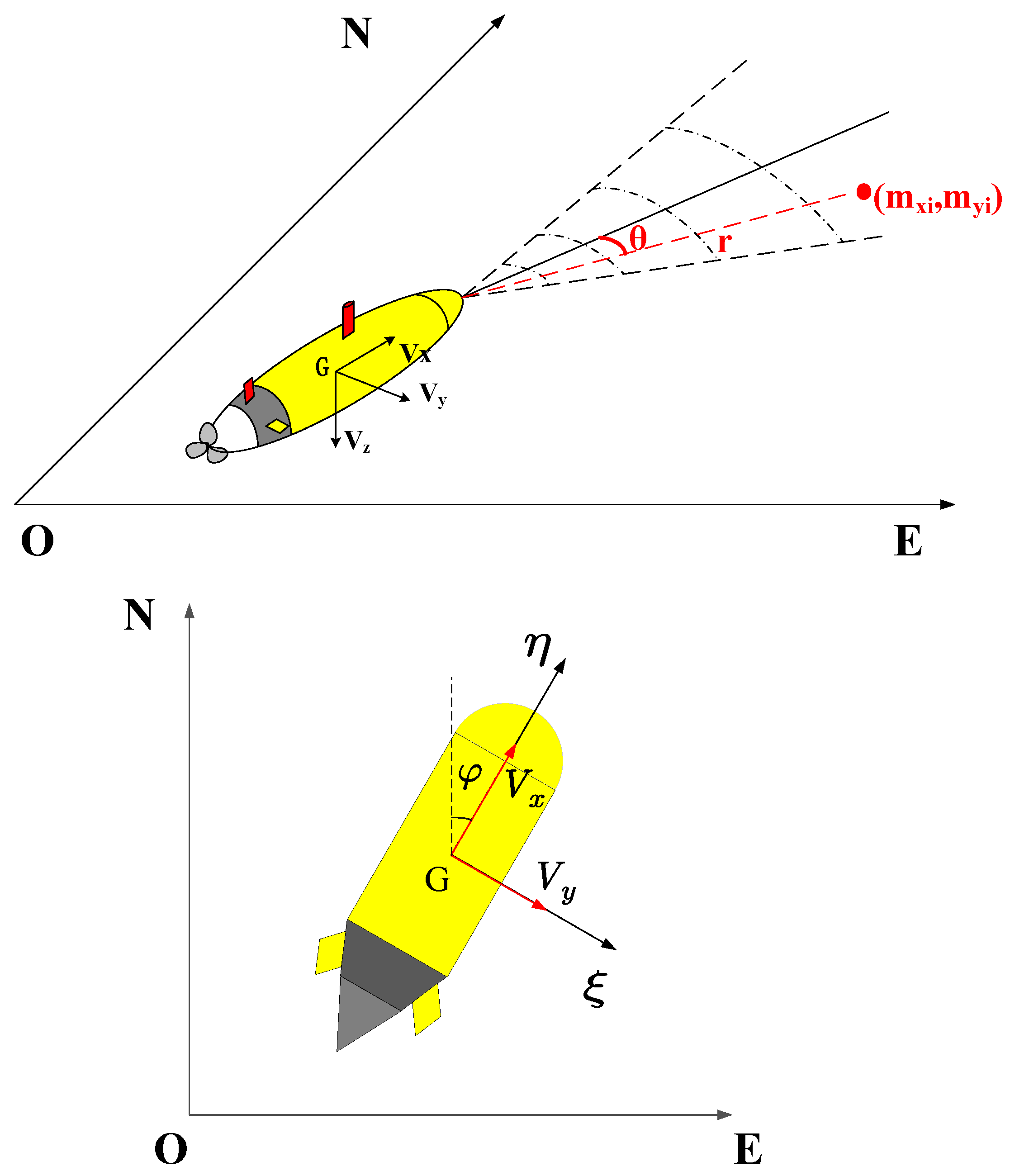
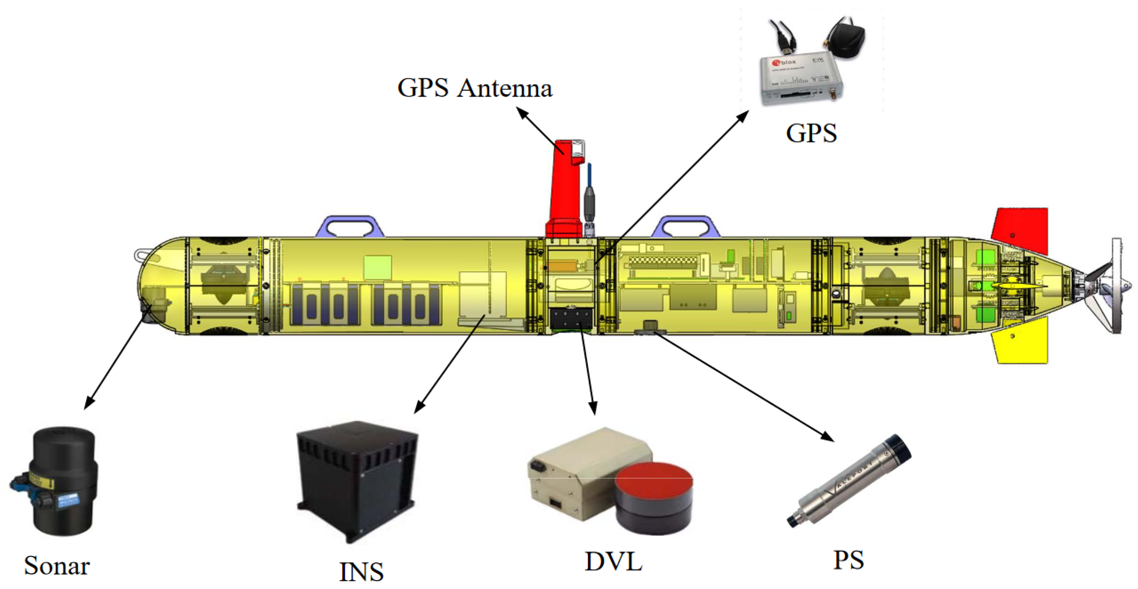
The Sailfish-210 is an independently developed AUV by the Underwater Vehicle Lab at Ocean University of China. The length of Sailfish-210 is 1.7 m, and the outer diameter of the cabin is 0.21 m. Maximum working depth can reach 200 m. The AUV can reach speeds of 5 knots and sail at 3 knots for over 8 h. Figure 1 shows the basic structure of Sailfish-210 and the sensors required for this experiment, and

Table 1. Specifications of sensors.

Sensors	Parameter	Value
INS	yaw	0.3° RMS
	Pitch, Roll	0.02° RMS
	Update Rate	100 Hz
DVL	Operational Altitude	0.2–89 m
	Sound Frequency	614.4 kHz
	Accuracy	±0.2 cm/s
GPS	Position Accuracy	2.5 m CEP
	Update Rate	1 Hz
PS	Accuracy	0.01% Range
	Update Rate	1 Hz
SONAR	Frequency	675 kHz
	Vertical beam width	30°
	Horizontal beam width	3°
	Detection distance	0.3–100 m

is the technical specifications of the sensors.

2.1.1. GPS

To accurately locate the Sailfish-210 AUV on the water surface and use it as a benchmark to evaluate the performance of different algorithms, the AUV is equipped with a high-precision, high-performance Global Positioning System (GPS) receiver. At the same time, a GPS filtering algorithm that has been proven to be effective in actual engineering was applied to this experiment.

2.1.2. Attitude Sensor

The INS equipped in Sailfish-210 AUV is HN-100, which mainly includes an inertial measurement unit. Through the acceleration and angular velocity obtained by the IMU, the position, velocity and attitude angle can be calculated.

2.1.3. Velocity Sensor

The speed measurement sensor used in this experiment is Pathfinder DVL, which works by sending sound waves to the seabed, and outputs the speed of the AUV in the carrier coordinate system by measuring the bottom three-axis speed and the distance to the bottom height fusion algorithm. DVL can obtain the speed of the carrier in real time without cumulative error. Therefore, during the experiment, the speed information measured by DVL is used as the current speed measurement value of the AUV.

2.1.4. Detection Sensor

Sonar is an essential external detection sensor for AUV SLAM. In this experiment, we choose Tritech small single-beam Mechanical Scanning Imaging Sonar (MSIS), which has the advantages of large detectable angle (0°–360°), small size, and lightweight (324 g in the air). Moreover, its farthest detection range can reach 100 m.

2.2. Auv Model Description

The AUV state vector consists of its position and yaw at time k, as shown in Equation (1), where ($x_k$, $y_k$) represent the coordinates of the AUV in the geographic coordinate system. ${\phi }_k$ represents the angle between the AUV direction and the geographic north direction, in the range of $\left[0°,360°\right)$. AUV rotates clockwise to increase direction of ${\phi }_k$. The map M consists of the coordinates of feature points, for example, ($m_{x_n}$, $m_{y_n}$) represent the coordinates of the n-th feature point in the geographic coordinate system. That is, $m_{x_n}$ represents $m_{x_n}$ meters away from the origin in the horizontal direction and $m_{y_n}$ represents $m_{y_n}$ meters from the origin in the vertical direction.

$$X_k={\left[x_k y_k {\phi }_k\right]}^T$$

(1)

$$M={\left[m_{x_1} m_{y_1}\cdots m_{x_n} m_{y_n}\right]}^T$$

(2)

The motion model of Sailfish-210 AUV can be expressed as Equation (3).

$$X_k=\left[\begin{array}{c}{x}_k\\ y_k\\ {\phi }_k\end{array}\right]=\left[\begin{array}{c}{x}_{k-1}+V_x·\Delta T·\cos \left({\phi }_{k-1}\right)-V_y·\Delta T·\sin \left({\phi }_{k-1}\right)\\ y_{k-1}+V_x·\Delta T·\sin \left({\phi }_{k-1}\right)+V_y·\Delta T·\cos \left({\phi }_{k-1}\right)\\ {\phi }_{k-1}+W·\Delta T\end{array}\right]+{\delta }_k$$

(3)

where $\Delta T$ represents the sampling interval, $V_x$ and $V_y$ represent the forward and starboard velocity of AUV respectively, ${\phi }_k$ denotes the yaw at the current moment and W represents the angular acceleration. ${\delta }_k$ represents system noise, and ${\delta }_k\sim N\left(0,Q_k\right)$, $Q_k$ represents its covariance matrix.

The observation model of AUV can be expressed as:

$$Z_{k,i}=\left[\begin{array}{c}{r}_{k,i}\\ {\theta }_{k,i}\end{array}\right]=\left[\begin{array}{c}\sqrt{{\left(m_{x_i}-x_k\right)}^2+{\left(m_{y_i}-y_k\right)}^2}\\ \mathrm{arc}\tan \frac{m_{y_i}-y_k}{m_{x_i}-x_k}-{\phi }_k\end{array}\right]+{\epsilon }_k$$

(4)

where $r_{k,i}$ and ${\theta }_{k,i}$ represent that the i-th feature point at time k is located r meters away from the AUV and rotated $\theta$° clockwise from the AUV direction. ${\epsilon }_k$ represents observation noise, and satisfies ${\epsilon }_k\sim N\left(0,R_k\right)$, $R_k$ represents its covariance matrix. The navigation coordinate system of Sailfish-210 AUV can be represented by Figure 2.

3. Improved AUV SLAM Algorithm

We take the VB-AUFastSLAM as an example to introduce our proposed algorithm. VB-UPF is used to estimate the posterior probability $p\left(S^k|z^k,u^k,n^k\right)$ of the AUV pose, and VB-UKF is used to estimate and update the features. We describe the algorithm with the model (Equations (3) and (4)) used by the Sailfish-210 AUV in this paper.

3.1. Vb-Based Sampling the New AUV Pose

For each particle, according to the UKF method, the state vector of the i-th particle is augmented with a control input. Assuming that the mean of the control noise is zero, the augmented state is formulated as:

$$X_{k-1}^{augment\left[i\right]}=\left[\begin{array}{c}{X}_{k-1}^{\left[i\right]}\\ \mathbf{0}\end{array}\right]=\left[\begin{array}{c}{x}_{k-1}^{\left[i\right]}\\ y_{k-1}^{\left[i\right]}\\ {\phi }_{k-1}^{\left[i\right]}\\ \mathbf{0}\end{array}\right]\hspace{1em}\in {\mathbb{R}}^6$$

(5)

$$\begin{array}{c}\hfill P_{k-1}^{augment\left[i\right]}=\left[\begin{array}{cc}{P}_{k-1}^{\left[i\right]}& \mathbf{0}\\ \mathbf{0}& Q_k\end{array}\right]\hspace{1em}\in {\mathbb{R}}^{6\times 6}\end{array}$$

(6)

here, $X_{k-1}^{augment\left[i\right]}$ is the augmented vector for the state, $X_{k-1}^{\left[i\right]}$ and $P_{k-1}^{\left[i\right]}$ denote the previous state and covariance. $Q_k$ denotes the process noise. $x_{k-1}^{\left[i\right]}$, $y_{k-1}^{\left[i\right]}$, ${\phi }_{k-1}^{\left[i\right]}$ respectively represent the X-axis position, Y-axis position and yaw of the AUV.

VB-AUFastSLAM extracts sigma points from the Gaussian and passes these points through the nonlinear function. A symmetric set of 2n + 1 sigma points ${\chi }_{k-1|k-1,j}^{augment\left[i\right]}$ for the augmented state vector can be given by:

$$\begin{array}{c}\hfill \left\{\begin{array}{c}{\chi }_{k-1|k-1,0}^{augment\left[i\right]}=X_{k-1}^{augment\left[i\right]}\hfill \\ {\chi }_{k-1|k-1,j}^{augment\left[i\right]}=X_{k-1}^{augment\left[i\right]}+{\left(\sqrt{\left(n+\lambda \right)P_{k-1}^{augment\left[i\right]}}\right)}_j ,j=1,2,\dots ,n\hfill \\ {\chi }_{k-1|k-1,j}^{augment\left[i\right]}=X_{k-1}^{augment\left[i\right]}-{\left(\sqrt{\left(n+\lambda \right)P_{k-1}^{augment\left[i\right]}}\right)}_j ,j=n+1,\dots ,2n\hfill \end{array}\right.,{\chi }_{k-1|k-1}^{augment\left[i\right]}\in {\mathbb{R}}^{6\times (2n+1)}\end{array}$$

(7)

where the $\lambda$ is computed by $\lambda ={\alpha }^2\left(n+\kappa \right)-n$. $\alpha$ is a small number to avoid sampling nonlocal effects ($\alpha =0.002$ is appropriate). $\kappa \left(\kappa >0\right)$ is used to determine the distance between the sigma points and the mean which is not critical though, so a good default choice is $\kappa =0$. j represents the j-th column of matrix $\sqrt{\left(n+\lambda \right)P_{k-1}^{augment\left[i\right]}}$. Each ${\chi }_{k-1|k-1}^{augment\left[i\right]}$ contains the state and control noise components given by:

$$\begin{array}{c}\hfill {\chi }_{k-1|k-1}^{augment\left[i\right]}=\left[\begin{array}{c}{\chi }_{k-1|k-1}^{\left[i\right]}\\ {\chi }_k^{u\left[i\right]}\end{array}\right]\hspace{1em}\in {\mathbb{R}}^{6\times (2n+1)}\end{array}$$

(8)

The weights corresponding to the state and the covariance can be calculated as:

$$\begin{array}{c}\hfill \left\{\begin{array}{c}{\omega }_m^0=\lambda /n+\lambda \hfill \\ {\omega }_c^0=\lambda /n+\lambda +\left(1-{\alpha }^2+\beta \right)\hfill \\ w_m^j={\omega }_c^j=1/2\left(n+\lambda \right) , j=1,2,\dots ,2n\hfill \end{array}\right.\end{array}$$

(9)

$\beta$ is the parameter used to introduce higher-order information items of the posterior probability distribution. For the Gaussian prior, the optimal choice is $\beta =2$.

The set of sigma points are transformed by the motion model characterized by a nonlinear function as follows:

$$\begin{array}{c}\hfill {\chi }_{k|k-1}^{\left[i\right]}=f\left({\chi }_{k-1|k-1}^{\left[i\right]},{\chi }_k^{u\left[i\right]}+u_k\right)=\left[\begin{array}{c}{\chi }_{k|k-1}^{x,\left[i\right]}\\ {\chi }_{k|k-1}^{y,\left[i\right]}\\ {\chi }_{k|k-1}^{\phi ,\left[i\right]}\end{array}\right]\hspace{1em}\in {\mathbb{R}}^3\end{array}$$

(10)

${\chi }_{k|k-1}^{\left[i\right]}$ is the transformed sigma point of the AUV state. The prediction state and the prediction state covariance matrix are calculated based on the weights as:

$$\begin{array}{c}\hfill X_{k|k-1}^{\left[i\right]}=\sum _{j=0}^{2n}{\omega }_m^j\times {\chi }_{k|k-1,j}^{\left[i\right]} , X_{k|k-1}^{\left[i\right]}\in {\mathbb{R}}^3\end{array}$$

(11)

$$\begin{array}{c}\hfill P_{k|k-1}^{\left[i\right]}=\sum _{j=0}^{2n}{\omega }_c^j\left({\chi }_{k|k-1,j}^{\left[i\right]}-X_{k|k-1}^{\left[i\right]}\right){\left({\chi }_{k|k-1,j}^{\left[i\right]}-X_{k|k-1}^{\left[i\right]}\right)}^T , P_{k|k-1}^{\left[i\right]}\in {\mathbb{R}}^{3\times 3}\end{array}$$

(12)

When external observations are available, the statistical characteristic of the time-varying observations noise covariance are estimated to improve the performance of algorithm. Since the Inverse-Gamma distribution is the conjugate prior distribution of the variance of the Gaussian distribution, in Bayesian analysis, the Inverse-Gamma model is usually chosen to model the variance of the Gaussian distribution [29]. $\eta$ and $\xi$ represent the hyper-parameters of Inverse-Gamma distribution, respectively. The Inverse-Gamma distribution is shown as Equation (13).

$$\begin{array}{c}\hfill Inverse-Gamma\left({\sigma }^2|\eta ,\xi \right)=\frac{{\xi }^{\eta }{\left({\sigma }^2\right)}^{-\left(\eta +1\right)}}{\Gamma \left(\eta \right)}\exp \left(-\frac{\xi }{{\sigma }^2}\right)\end{array}$$

(13)

We introduce the VB method to approximate the observation noise. Based on VB, the joint posterior estimation of the system state $X_{k|k}^{\left[i\right]}$ and the observation noise covariance $R_{k|k}^{\left[i\right]}$ can be expressed as:

$$\begin{array}{c}\hfill f\left(x_k,R_k|z_k\right)=Q_x\left(x_k\right)Q_R\left(R_k\right)\end{array}$$

(14)

where $Q_x\left(x_k\right)$ and $Q_R\left(R_k\right)$ are the approximate probability distributions of the state vector and observation noise parameters, respectively. The VB approximation can be formed by minimizing the Kullback–Leibler (KL) divergence between the true distribution and the approximation:

$$\begin{array}{cc}\hfill & KL\left[Q_X\left(x_k\right)Q_R\left(R_k\right)\left|\right|f\left(x_{k|k},R_k|z_k\right)\right]\hfill \\ \hfill =& \int Q_X\left(x_k\right)Q_R\left(R_k\right)\log \frac{Q_X\left(x_k\right)Q_R\left(R_k\right)}{f\left(x_{k|k},R_{k|k}|z_k\right)}d{x}_{k|k}d{R}_{k|k}\hfill \end{array}$$

(15)

When minimizing the KL divergence, fixing $Q_X\left(x_k\right)$ or $Q_R\left(R_k\right)$ respectively, the following can be obtained:

$$\begin{array}{c}\hfill Q_X\left(x_k\right)\propto \exp \left(\int Q_R\left(R_k\right)\log f\left(x_k,z_k,R_k|z_{1:k-1}\right)d{R}_k\right)\\ \hfill Q_R\left(R_k\right)\propto \exp \left(\int Q_X\left(x_k\right)\log f\left(x_k,z_k,R_k|z_{1:k-1}\right)d{x}_k\right)\end{array}$$

(16)

As the above equations are coupled, it cannot be solved directly, after computing the expectations separately, we can obtain:

$$\begin{array}{c}\hfill \int Q_R\left(R_k\right)logf\left(x_k,z_k,R_k|z_{1:k-1}\right)d{R}_k\\ \hfill =-\frac{1}{2}{\left(z_k-h\left(x_k\right)\right)}^T〈R_k^{-1}〉\left(z_k-h\left(x_k\right)\right)\\ \hfill -\frac{1}{2}{\left(x_k-x_{k|k-1}\right)}^T{\left(P_{k|k-1}\right)}^{-1}\left(x_k-x_{k|k-1}\right)+c_1\end{array}$$

(17)

where $〈·〉=\int Q_R\left(R_k\right)\left(·\right)d{R}_k$ denotes the expected value with respect to the approximating distribution $Q_R\left(R_k\right)$. As a function of $x_k$, this is a quadratic implying that $Q_X\left(x_k\right)$ is a Gaussian distribution, both the mean and variance can be obtained by standard matrix operations.

Similarly, the expectation of $Q_R\left(R_k\right)$ can be calculated as follows:

$$\begin{array}{c}\hfill \int Q_X\left(x_k\right)logf\left(x_k,z_k,R_k|z_{1:k-1}\right)d{x}_k\\ \hfill =-\sum _{i=1}^d\left(3/2+{\eta }_{k,i}\right)ln\left({\sigma }_{k,i}^2\right)-\sum _{i=1}^d\frac{{\xi }_{k,i}}{{\sigma }_{k,i}^2}\\ \hfill -\frac{1}{2}\sum \frac{1}{{\sigma }_{k,i}^2}〈{\left(z_k-h\left(x_k\right)\right)}^2〉+c_2\end{array}$$

(18)

where $〈·〉=\int Q_X\left(x_k\right)\left(·\right)d{x}_k$. From the above equation, it can be seen that $Q_R\left(R_k\right)$ is the product of the Inverse-Gamma distribution. If we assume that $R_k$ is d-dimensional, then $R_k$ can be expressed as:

$$\begin{array}{c}\hfill R_k=\mathrm{diag}\left({\xi }_{k,1}/{\eta }_{k,1},...,{\xi }_{k,d}/{\eta }_{k,d}\right)\hspace{1em}\in {\mathbb{R}}^{d\times d}\end{array}$$

(19)

To ensure that the joint predicted probability distribution of $R_k$ at time k keeps the same form as the posterior probability distribution at time $k-1$, a forgetting factor $\rho ϵ \left(0,1\right)$ is introduced to reflect the degree of fluctuation of the noise. The prior of the observation noise parameters can be expressed as:

$$\begin{array}{c}\hfill {\eta }_{k|k-1,j}=\rho {\eta }_{k-1|k-1,j}\end{array}$$

(20)

$$\begin{array}{c}\hfill {\xi }_{k|k-1,j}=\rho {\xi }_{k-1|k-1,j}\end{array}$$

(21)

The exact observation noise posterior distribution is obtained cyclically and iteratively during the observation update. It should be emphasized that the loop iteration of the observation noise using the VB method is performed on the covariance matrix, so the observation noise still satisfies the Gaussian white noise distribution, i.e., $R_{k|k}^{*}\sim N\left(0,R_k\right)$.

As feature points are observed and matched with existing features after data association, the following stage will be employed to iterative update the $X_{k|k}^{\left[i\right]}$ and the covariance $P_{k|k}^{\left[i\right]}$ of the robot. From the observation model, the predicted observation of the sigma points can be calculated as:

$$\begin{array}{c}\hfill {\overline{z}}_{k|k-1,j}^{\left[i\right]}=h\left({\chi }_{k|k-1,j}^{\left[i\right]}\right) , {\overline{z}}_{k|k-1,j}^{\left[i\right]}\in {\mathbb{R}}^2\end{array}$$

(22)

The predicted observation and cross-covariance matrix can be obtained as:

$$\begin{array}{c}\hfill Z_{k|k-1}^{\left[i\right]}=\sum _{j=0}^{2n}{\omega }_m^j\times {\overline{z}}_{k|k-1,j}^{\left[i\right]} , Z_{k|k-1}^{\left[i\right]}\in {\mathbb{R}}^2\end{array}$$

(23)

$$\begin{array}{c}\hfill P_{xz,k|k-1}^{\left[i\right]}=\sum _{j=0}^{2n}{w}_c^j\left({\chi }_{k|k-1,j}^{\left[i\right]}-X_{k|k-1}^{\left[i\right]}\right){\left({\overline{z}}_{k|k-1,j}^{\left[i\right]}-Z_{k|k-1}^{\left[i\right]}\right)}^T , P_{xz,k|k-1}^{\left[i\right]}\in {\mathbb{R}}^{3\times 2}\end{array}$$

(24)

The mean and covariance of the state vector are calculated as:

$$\begin{array}{c}\hfill S_k^{\left[i\right]}=\sum _{j=0}^{2n}{w}_c^j\left({\overline{z}}_{k|k-1}^{\left[i\right]}-Z_{k|k-1}^{\left[i\right]}\right){\left({\overline{z}}_{k|k-1}^{\left[i\right]}-Z_{k|k-1}^{\left[i\right]}\right)}^T , S_k^{\left[i\right]}\in {\mathbb{R}}^{2\times 2}\end{array}$$

(25)

$$\begin{array}{c}\hfill P_{zz,k|k}^{\left[i\right]}=S_k^{\left[i\right]}+R_{k|k}^{*} , P_{zz,k|k}^{\left[i\right]}\in {\mathbb{R}}^{2\times 2}\end{array}$$

(26)

$$\begin{array}{c}\hfill K_k^{\left[i\right]}=P_{xz,k|k-1}^{\left[i\right]}{\left(P_{zz,k|k}^{\left[i\right]}\right)}^{-1} , K_k^{\left[i\right]}\in {\mathbb{R}}^{3\times 2}\end{array}$$

(27)

$$\begin{array}{c}\hfill X_{k|k}^{\left[i\right]}=X_{k|k-1}^{\left[i\right]}+K_k^{\left[i\right]}\left(Z_k-Z_{k|k-1}^{\left[i\right]}\right)\end{array}$$

(28)

$$\begin{array}{c}\hfill P_{k|k}^{\left[i\right]}=P_{k|k-1}^{\left[i\right]}-K_k^{\left[i\right]}{\left[S_k^{\left[i\right]}+R_{k|k}^{*}\right]}^{-1}{\left(K_{k|k}^{\left[i\right]}\right)}^T\end{array}$$

(29)

What needs to be noted here that the observation noise $R_{k|k}^{*}$ at this time has been modeled as an Inverse-Gamma distribution. Furthermore $R_{k|k}^{*}$ denotes the temporary value during the filtering loop, when the loop ends, save the final estimated noise of this observation:

$$\begin{array}{c}\hfill R_{k|k}^{\left[i\right]\left[j\right]}=R_{k|k}^{*}\end{array}$$

(30)

where i represents the i-th particle and j represents the observed noise for the j-th feature. The noise of each observed feature is estimated and $R_{k|k}^{\left[i\right]\left[j\right]}$ will be used in the subsequent mapping stage. Moreover, the update of the noise hyper-parameters can be expressed as:

$$\begin{array}{c}\hfill {\eta }_{k|k}^{\left[i\right]}={\eta }_{k|k-1}^{\left[i\right]}+\left(1/2,...,1/2\right)\hspace{1em},\hspace{1em}{\eta }_{k|k}^{\left[i\right]}\in {\mathbb{R}}^2\end{array}$$

(31)

$$\begin{array}{c}\hfill {\xi }_{k|k}^{\left[i\right]}={\xi }_{k|k-1}^{\left[i\right]}+{\left(Z_k-Z_{k|k-1}^{\left[i\right]}\right)}^2+\mathrm{diag}\left(S_k^{\left[i\right]}/2\right)\hspace{1em},\hspace{1em}{S}_k^{\left[i\right]}\in {\mathbb{R}}^2\end{array}$$

(32)

3.2. Feature State Estimation by VB-UKF

Based on $X_{k|k}^{\left[i\right]}$ known in Section 3.1, feature state estimation in VB-AUFastSLAM can be divided into two parts: the feature update stage and feature augmentation stage.

(1) Feature augmentation

Since the path at time k is known, the observation noise can be used as the initial feature covariance matrix, so that in the mapping stage of the VB-AUFastSLAM, current observation $Z_k$ and the observation noise covariance matrix are chosen as the initial inputs, we can obtain the sigma point of the observation as:

$$\begin{array}{c}\hfill \left\{\begin{array}{c}{\Gamma }_{k-1|k-1,0}^{\left[i\right]}=Z_k\hfill \\ {\Gamma }_{k-1|k-1,j,}^{\left[i\right]}=Z_k+\left(\sqrt{\left(n+\lambda \right)R_{k|k}}\right) j=1,\dots ,l\hfill \\ {\Gamma }_{k-1|k-1,j,}^{\left[i\right]}=Z_k-\left(\sqrt{\left(n+\lambda \right)R_{k|k}}\right) j=l+1,\dots ,2l\hfill \end{array}\right.\hspace{1em},\hspace{1em}{\Gamma }_{k-1|k-1}^{\left[i\right]}\in {\mathbb{R}}^{2\times (2l+1)}\end{array}$$

(33)

where $\lambda ={\alpha }^2\left(n+\kappa \right)-n$, in the feature update stage, it is usually set $\alpha =0.001,\kappa =0$. After nonlinear transformation, the mean and covariance of the new features can be obtained as follows:

$$\begin{array}{c}\hfill Y_{k|k-1,j}^{\left[i\right]}=h^{-1}\left({\Gamma }_{k-1|k-1,j}^{\left[i\right]},X_{k|k}^{\left[i\right]}\right) j=0,\dots ,2l\hspace{1em},\hspace{1em}{Y}_{k|k-1,j}^{\left[i\right]}\in {\mathbb{R}}^2\end{array}$$

(34)

$$\begin{array}{c}\hfill X_{k|k-1}^{f,\left[i\right]}=\sum _{j=0}^{2l}{w}_m^j{Y}_{k|k-1,j}^{\left[i\right]}\hspace{1em},\hspace{1em}{X}_{k|k-1}^{f,\left[i\right]}\in {\mathbb{R}}^2\end{array}$$

(35)

$$\begin{array}{c}\hfill P_{k|k-1}^{f,\left[i\right]}=\sum _{j=0}^{2l}{w}_c^j\left(Y_{k|k-1,j}^{\left[i\right]}-X_{k|k-1}^{f,\left[i\right]}\right){\left(Y_{k|k-1,j}^{\left[i\right]}-X_{k|k-1}^{f,\left[i\right]}\right)}^T\hspace{1em},\hspace{1em}{P}_{k|k-1}^{f,\left[i\right]}\in {\mathbb{R}}^{2\times 2}\end{array}$$

(36)

(2) Feature update

Feature points will be updated after feature matching is completed. We convert the feature points position to sigma points as:

$$\begin{array}{c}\hfill \left\{\begin{array}{c}{\chi }_{k|k-1,0}^{f,\left[i\right]}=X_{k|k-1}^{f,\left[i\right]}\hfill \\ {\chi }_{k|k-1,j}^{f,\left[i\right]}=X_{k|k-1}^{f,\left[i\right]}+\left(\sqrt{\left(n+\lambda \right)P_{k|k-1}^{f,\left[i\right]}}\right) j=1,\dots ,n\hfill \\ {\chi }_{k|k-1,j}^{f,\left[i\right]}=X_{k|k-1}^{f,\left[i\right]}-\left(\sqrt{\left(n+\lambda \right)P_{k|k-1}^{f,\left[i\right]}}\right) j=n+1,\dots ,2n\hfill \end{array}\right.\end{array}$$

(37)

According to the $X_{k|k}^{\left[i\right]}$ at time k and the nonlinear observation model $h\left(·\right)$, the predicted observations can be obtained:

$$\begin{array}{c}\hfill {\overline{z}}_{k|k-1,j}^{f,\left[i\right]}=h\left({\chi }_{k|k-1,j}^{f,\left[i\right]},X_{k|k}^{\left[i\right]}\right)\hspace{1em}j=1,\dots ,2n,\hspace{1em}{\overline{z}}_{k|k-1,j}^{f,\left[i\right]}\in {\mathbb{R}}^2\end{array}$$

(38)

$$\begin{array}{c}\hfill Z_{k|k-1}^{f,\left[i\right]}=\sum _{j=0}^{2n}{\omega }_m^j\times {\overline{z}}_{k|k-1,j}^{f,\left[i\right]}\hspace{1em},\hspace{1em}{Z}_{k|k-1}^{f,\left[i\right]}\in {\mathbb{R}}^2\end{array}$$

(39)

$$\begin{array}{c}\hfill P_{xz,k|k-1}^{f,\left[i\right]}=\sum _{j=0}^{2n}{w}_c^j\left({\chi }_{k|k-1,j}^{f,\left[i\right]}-X_{k|k-1,j}^{f,\left[i\right]}\right){\left({\overline{z}}_{k|k-1,j}^{f,\left[i\right]}-Z_{k|k-1}^{f,\left[i\right]}\right)}^T\end{array}$$

(40)

$P_{xz,k|k-1}^{\left[i\right]}\in {\mathbb{R}}^{2\times 2}$ is the cross-covariance between state and observation in the feature update stage, which is used to compute the Kalman gain $K_k^{\left[i\right]}$:

$$\begin{array}{c}\hfill S_k^{f,\left[i\right]}=\sum _{j=0}^{2n}{w}_c^j\left({\overline{z}}_{k|k-1,j}^{f,\left[i\right]}-Z_{k|k-1}^{f,\left[i\right]}\right){\left({\overline{z}}_{k|k-1,j}^{f,\left[i\right]}-Z_{k|k-1}^{f,\left[i\right]}\right)}^T\hspace{1em},\hspace{1em}{S}_k^{f,\left[i\right]}\in {\mathbb{R}}^{2\times 2}\end{array}$$

(41)

$$\begin{array}{c}\hfill P_{zz,k|k}^{f,\left[i\right]}=S_k^{f,\left[i\right]}+R_{k|k}^{\left[i\right]\left[j\right]}\hspace{1em},\hspace{1em}{P}_{zz,k|k}^{f,\left[i\right]}\in {\mathbb{R}}^{2\times 2}\end{array}$$

(42)

$$\begin{array}{c}\hfill K_k^{f,\left[i\right]}=P_{xz,k|k-1}^{f,\left[i\right]}{\left(P_{zz,k|k}^{f,\left[i\right]}\right)}^{-1}\hspace{1em},\hspace{1em}{K}_k^{f,\left[i\right]}\in {\mathbb{R}}^{2\times 2}\end{array}$$

(43)

Similar to the path estimation stage, when calculating the innovation covariance $P_{zz,k|k}^{\left[i\right]}$, the observation noise $R_{k|k}$ needs to be estimated by the VB method. The difference is that the initial observation noise $R_{k|k}^{\left[i\right]\left[j\right]}$ in the feature update stage is already obtained from the path estimation stage, so the observation noise requires fewer cycles than the path estimation stage. After loop iteration, the position and covariance of the feature can be obtained:

$$\begin{array}{c}\hfill X_{k|k}^{f,\left[i\right]}=X_{k|k-1}^{f,\left[i\right]}+K_k^{f,\left[i\right]}\left(Z_k-Z_{k|k-1}^{f,\left[i\right]}\right)\end{array}$$

(44)

$$\begin{array}{c}\hfill P_{k|k}^{f,\left[i\right]}=P_{k|k-1}^{f,\left[i\right]}-K_k^{f,\left[i\right]}{\left[S_k^{f,\left[i\right]}+R_{k|k}\right]}^{-1}{\left(K_k^{f,\left[i\right]}\right)}^T\end{array}$$

(45)

3.3. Calculating Importance Weights and Resampling

Considering the latest observations in the proposed distribution, the weight calculation can be expressed by Equations (46) and (47):

$$\begin{array}{c}{W}_k^{\left[i\right]}={\left|2\pi L_k^{\left[i\right]}\right|}^{-\frac{1}{2}}\ast \exp \left\{-\frac{1}{2}{\left(Z_k-Z_{k|k-1}^{\left[i\right]}\right)}^T{\left(L_k^{\left[i\right]}\right)}^{-1}\left(Z_k-Z_{k|k-1}^{\left[i\right]}\right)\right\}\hfill \end{array}$$

(46)

$$\begin{array}{cc}\hfill L_k^{\left[i\right]}& ={\left(P_{xz,k|k-1}^{\left[i\right]}\right)}^T{P}_{k|k}^{\left[i\right]}\left(P_{xz,k|k-1}^{\left[i\right]}\right)+P_{zz,k|k}^{f,\left[i\right]}\hfill \end{array}$$

(47)

The particles with high weights are replicated, and the ones with low weights are thrown away. However, excessive resampling will lead to a reduction in particle diversity, resulting in particle depletion. To avoid redundant resampling steps, the effective number of particles ($N_{eff}$) is utilized as a criterion:

$$\begin{array}{c}\hfill N_{eff}=\frac{1}{{\sum }_{i=1}^N\left(W_k^{\left[i\right]}\right)}\end{array}$$

(48)

where N is the number of particles. $N_{eff}$ is set to 75% of the total number of particles in simulation tests and marine environment tests. If the effective particles are less than 75% of the total number of particles, resampling will be performed.

4. Simulations and Result Discussion

We first evaluate the effectiveness of the proposed algorithms in the simulation environment. We built a simulation map in Figure 3 based on the open-source simulation environment [30] presented by Tim. The robot trajectory path is specified by 20 waypoints with 127 landmarks and starts off at (0,0).

We additionally propose the VB-AFastSLAM algorithm based on FastSLAM, which has the same idea as VB-AUFastSLAM in Section 3, and compare the two proposed algorithms with FastSLAM and UFastSLAM. The initial observation noise covariance $R_0$ during the simulation is set to $R_0=\mathrm{diag}\left[0.001,0.001\right]$, other parameters are shown in

Table 2. Parameters and initial values of the experiments.

Parameter	Value/Initial Value
$\rho$	0.99
$\xi$	5
$\eta$	50

. To simulate dynamic noise, we modify the observation noise covariance as

Table 3. Add dynamic observation noise.

For each observation noise

If rand (1) < p

$R=n{R}_0$

end

end

.

Where p represents the probability of abnormal noise, n represents the degree of abnormal noise mutation. Changing p and n respectively to simulate the degree of the fluctuation of observed noise during the simulation. For each case, we have performed 30 Monte Carlo simulation experiments.

The n is set to fixed and p is varying to simulate the frequency of anomalous observation noise, and the simulation results are shown in

Table 4. n is constant, p increases.

		Comparison of RMSE of Each Algorithm (m)
		FastSLAM	UFastSLAM	VB-AFastSLAM	VB-AUFastSLAM
n = 2; p = 0.1	Path	2.770478	3.19563	1.625358	2.054199
	Path-X	0.855839	0.90384	1.132222	0.709995
	Path-Y	2.603047	3.05317	1.100274	1.847457
	Feature	9.279883	10.697	6.331278	6.836124
n = 2; p = 0.2	Path	5.669323	5.41272	2.833715	2.058928
	Path-X	1.522571	1.45913	1.204661	0.751841
	Path-Y	5.454597	5.21	2.431579	2.023639
	Feature	18.99598	18.1438	9.548879	6.838111
n = 2; p = 0.3	Path	8.76245	8.147479	3.158763	2.102712
	Path-X	2.33123	2.152331	1.443748	0.666417
	Path-Y	8.4435	7.856657	2.754322	1.719888
	Feature	29.3846	27.32396	10.19954	6.18904
n = 2; p = 0.4	Path	11.2517	10.77547	2.966079	2.064112
	Path-X	2.9615	2.816575	1.320611	0.794151
	Path-Y	10.8513	10.39766	2.507738	2.017267
	Feature	37.7403	36.13094	9.735261	7.237978
n = 2; p = 0.5	Path	13.7324	12.8347	2.895683	2.166283
	Path-X	3.57152	3.358806	1.268361	0.693661
	Path-Y	13.2565	12.38438	2.483241	1.718042
	Feature	46.0479	43.03384	9.572176	7.156179

. Where Path denotes the position error, Path-x, Path-y represent the northward and eastward error of the position respectively, and Feature displays the error of mapping. It can be seen from the Table 4 that the performance of VB-AFastSLAM and VB-AUFastSLAM are far better than traditional methods, of which VB-AUFastSLAM performs the best, and VB-AFastSLAM is the second. As the frequency of anomalous noise increases, the performance of the traditional algorithms deteriorates, in contrast, the error of our proposed algorithms remain stable.

Keeping p constant and at a low probability, n is varied to simulate the stability of each algorithm for abrupt observed noise, and the comparison results are shown in

Table 5. p is constant, n increases.

		Comparison of RMSE of Each Algorithm (m)
		FastSLAM	UFastSLAM	VB-AFastSLAM	VB-AUFastSLAM
n = 2; p = 0.2	Path	5.669323	5.41272	2.833715	2.058928
	Path-X	1.522571	1.45913	1.204661	0.751841
	Path-Y	5.454579	5.21	2.431579	2.023639
	Feature	18.99598	18.1438	9.548879	6.838111
n = 3; p = 0.2	Path	8.57249	7.840694	2.556053	2.149585
	Path-X	2.26609	2.187815	1.266831	0.6415
	Path-Y	8.26531	7.522545	2.100756	1.707999
	Feature	28.7391	26.30187	8.405979	6.906663
n = 4; p = 0.2	Path	12.26886	11.3883	2.734613	2.019741
	Path-X	3.18036	3.05627	1.175704	0.673702
	Path-Y	11.847	10.9659	2.318934	1.672129
	Feature	41.14187	38.2046	9.484266	6.615162
n = 5; p = 0.2	Path	15.42614	16.1654	2.797301	2.14828
	Path-X	4.047595	4.21373	1.273138	0.705636
	Path-Y	14.88411	15.6039	2.345235	1.512899
	Feature	51.73779	54.2395	10.15373	6.941755
n = 6; p = 0.2	Path	18.62159	18.0894	2.797817	2.102595
	Path-X	4.893386	4.85773	1.275668	0.737804
	Path-Y	17.96376	17.4199	2.395613	1.746299
	Feature	62.4486	60.6946	10.03549	6.681115

. In this case, we can arrive at the same conclusion. Especially when the noise is extremely abnormal, such as n = 6; p = 0.2, both VB-AFastSLAM and VB-AUFastSLAM show excellent noise adaptability. Figure 4 shows the performance comparison of the four algorithms with less anomalous noise and fewer occurrences (n = 2; p = 0.3), where the blue trajectory is obtained by the algorithm and the red points represent the estimated features. Figure 5 is the error comparison diagram of the whole process.

Too many invalid particles are the main cause of particle depletion. The number of effective particles is another important criterion for judging RBPF-SLAM. Figure 6 shows the comparison of effective particle numbers of the four algorithms. $N_{eff}$ is calculated according to Equation (48), and the $N_{eff}$ of each algorithm under each type of noise is the average of 30 simulation results. As the noise gradually increases, the average effective particles of VB-AUFastSLAM and VB-AFastSLAM are higher and remain stable, showing good adaptiveness to dynamic noise. The traditional algorithms have fewer effective particles than the proposed algorithms when there are no anomalous noise. As the random abnormal noise increases, the number of effective particles decreases gradually, and the error increases accordingly.

The above dynamic noise experiments show that the proposed two algorithms are significantly better than the traditional ones. We also verify the performance of the proposed algorithms under large initialization errors. As shown in

Table 6. RMSE comparison with large error initialization (m).

		Dynamic Observation Noise Is Set to n = 2; p = 0.3
		$\mathbf{\eta }=\mathbf{50},\mathbf{\xi }=\mathbf{10}$	$\mathbf{\eta }=\mathbf{50},\mathbf{\xi }=\mathbf{20}$	$\mathbf{\eta }=\mathbf{50},\mathbf{\xi }=\mathbf{30}$	$\mathbf{\eta }=\mathbf{50},\mathbf{\xi }=\mathbf{40}$	$\mathbf{\eta }=\mathbf{50},\mathbf{\xi }=\mathbf{50}$
VB-AFastSLAM	Path	3.221525	3.223039	3.406439	3.470573	3.472635
	Path-X	1.446131	1.317321	1.446759	1.259249	1.310155
	Path-Y	2.775732	2.758277	2.947062	3.171144	3.125832
	Feature	10.5447	11.20574	11.2116	11.24503	11.47512
VB-AUFastSLAM	Path	2.122799	2.579016	2.789813	2.794172	2.863803
	Path-X	0.994603	1.0425	1.064196	0.960737	1.030024
	Path-Y	1.896949	2.39992	2.546568	2.529119	2.578043
	Feature	7.021528	8.131228	9.188775	9.227863	9.734567

, it represents the corresponding performance when $\eta$ and $\xi$ are initialized to different parameters. The initial observation noise covariance (obtained by Equation (19)) is in the range of 0.2 to 1, which is much higher than the basic R = diag[0.001, 0.001]. By setting different initialization parameters and conducting experiments under the condition that the observation noise is n = 2, p = 0.3, it can be found from Table 6 that the performance of the two proposed algorithms decreases with the increase of the initialization error, but still within the normal range.

Remark1. 

According to Equations (20) and (21), ρ represents the degree of fluctuation of the observation noise, with a larger ρ representing a smaller degree of noise fluctuation. According to Equation (19), η and ξ are two variables that directly affect the initialization of observation noise. According to Equation (31), η increases by a fixed amount during the iteration process. We have found in many experiments that a larger value of η will achieve relatively good results, and ξ should be set much smaller than η. If ξ and η are similar, then will lead to an increase in filtering error.

The running time of the SLAM algorithm is also an important index.

Table 7. Running time comparison.

	FastSLAM	UFastSLAM	VB-AFastSLAM	VB-AUFastSLAM
Running time (s)	76.8727	103.7898	92.1792	126.9096

shows running time comparison of four algorithms. It can be seen from Table 7 that due to the use of the UKF-based method, VB-AUFastSLAM performs a large number of UT transformations, resulting in a large increase in running time compared to VB-AFastSLAM. Compared with their respective basic algorithms, VB-AFastSLAM and VB-AUFastSLAM increase the running time by 19.91% and 22.36%. Compared with UFastSLAM, the running time of VB-AFastSLAM is reduced by 11.19%. Therefore, the amount of time to perform calculations has increased a little. That can be ignored against the high accuracy obtained.

5. Sea Trial Results and Analysis

In this section, we compare the two proposed algorithms with traditional algorithms on the Sailfish-210 AUV platform.

5.1. Experiment Description

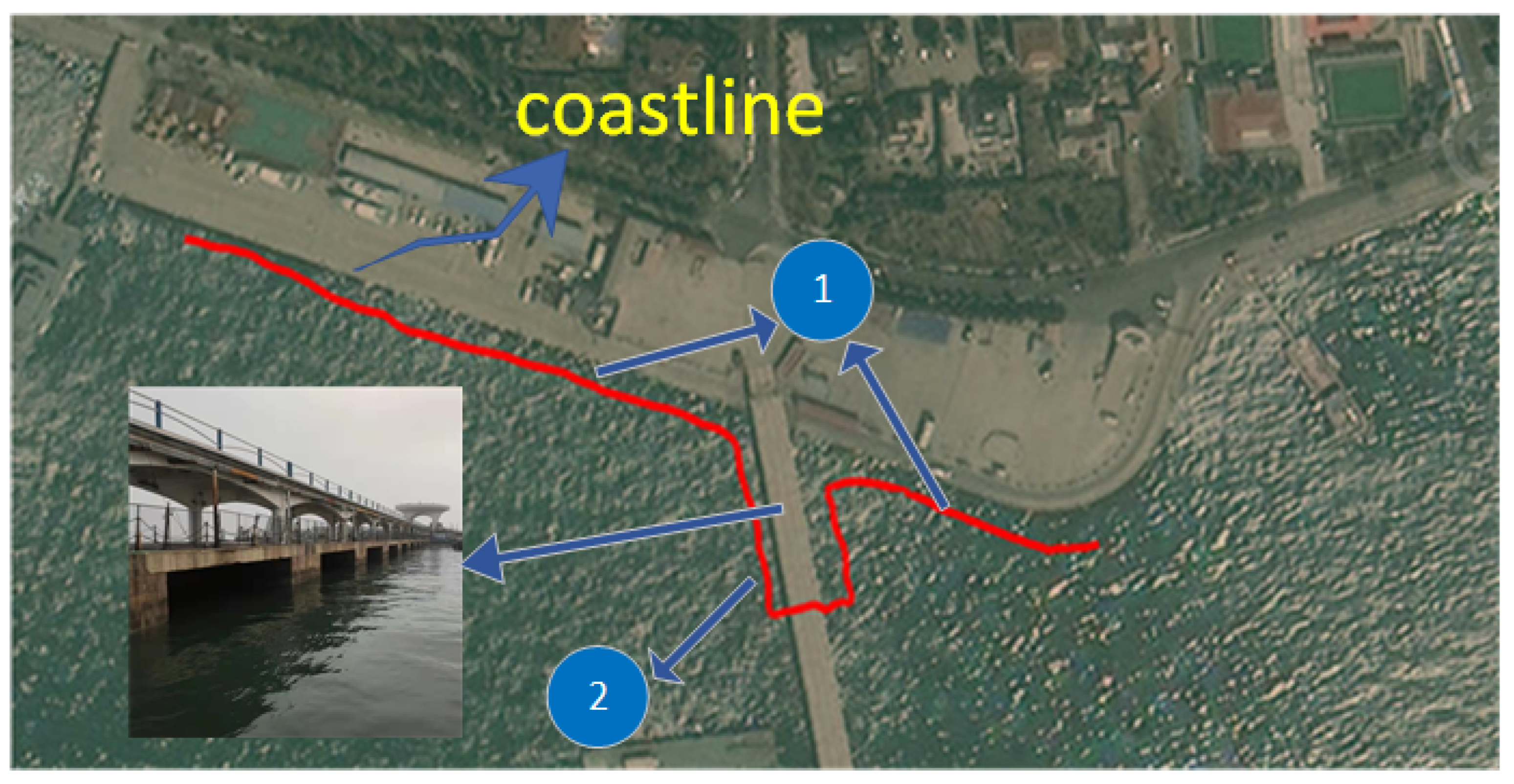
The experimental area is around 36.05° N, 120.29° E, Tuandao, Qingdao and the experimental site is shown in Figure 7. The red line represents the trajectory of the AUV. The AUV first sailed along the coastline, then sailed along the bridge shown in the figure, and finally passed through the bridge hole to continue sailing on the east side of the bridge. In order to distinguish clearly, we name the path along the coastline as path 1 and the path along the bridge as path 2. During the whole experiment, by reducing the buoyancy, the rest of the AUV was immersed in the water except the antenna and the rudder. The scanning sonar is located about 25 cm below the water surface. The advantage of this is that it does not affect the normal operation of the sonar. Accurate GPS data will also be obtained. The GPS data are only used to verify the accuracy of the algorithms and will not be applied to AUV navigation. The sailfish-210 during the experiment is shown in Figure 8.

We use Nearest Neighbor (NN) to achieve data association in this experiment. First, set an association gate according to the predicted position of the feature to be associated to limit the number of potential observation decisions, and the candidate observations are preliminarily screened out by the association gate. Then, calculate the Mahalanobis distance between the observation and each feature according to Equation (49).

$$\begin{array}{c}\hfill D={\left(Z_k-Z_{k|k-1}^{f,\left[i\right]}\right)}^T{S}_k^{f,\left[i\right]}\left(Z_k-Z_{k|k-1}^{f,\left[i\right]}\right)\end{array}$$

(49)

where $S_k^{f,\left[i\right]}$ can be obtained by Equation (41). The observation with the smallest Mahalanobis distance is regarded as the observation generated by the feature. The most significant advantage of using this method is the low computational complexity of only O(M), where M is the number of features contained in the state. Furthermore, this method has been successfully applied in the field of AUV SLAM.

5.2. Results and Analysis

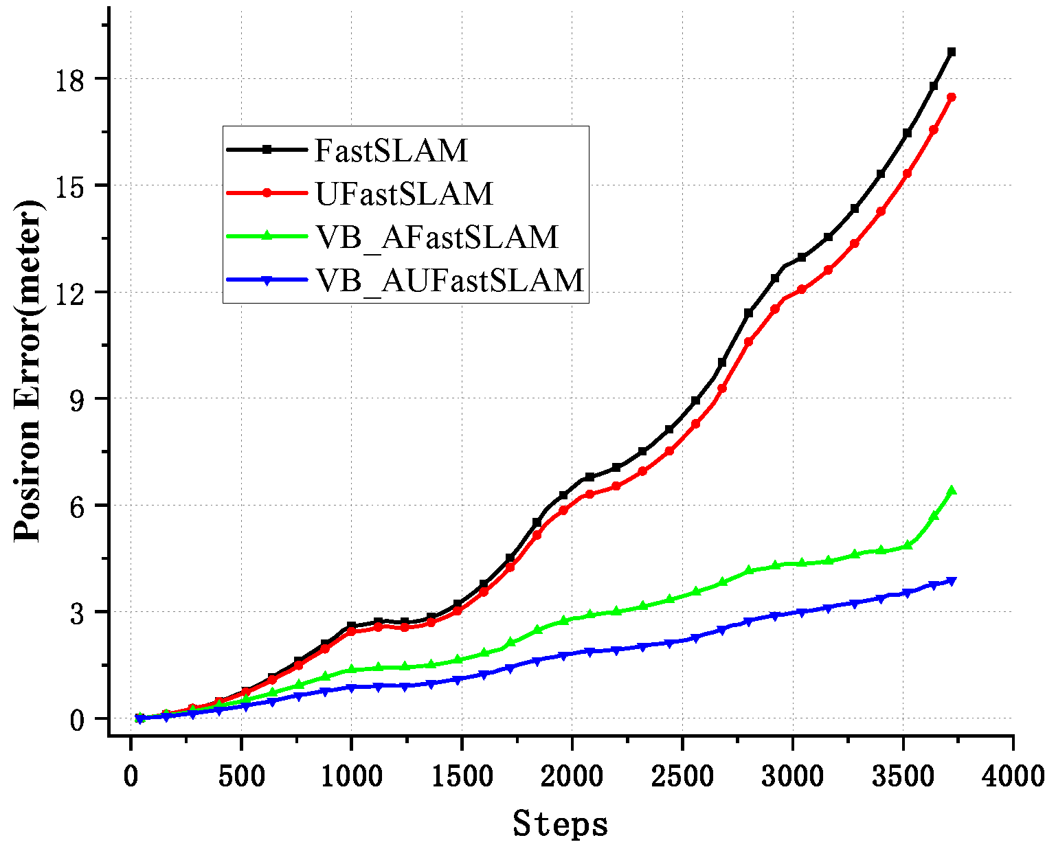
In this experiment, the sailing distance is 361.5643 m. Figure 9a is a comparison of the paths of the four algorithms, where the black line represents the GPS trajectory after wild value filtering as the true value, and the comparison shows that the trajectories of VB-AUFastSLAM and VB-AFastSLAM fit the GPS trajectory better. After calculating the error of each algorithm and GPS trajectory separately, we obtain Figure 9b. “steps” represents the sampling period, in this experiment, our data was recorded at a frequency of 10 Hz, where data points 1 to 1800 and 3600 to the end indicate that the AUV sails along the coastline, i.e., path 1 in Figure 7, and data points 1800 to 3600 indicate that the AUV sails along the bridge, i.e., path 2 in Figure 7. During the movement of the AUV in path 1, the sonar can always detect the wall along the coast. Since the sonar is affected by dynamic ocean noise and self-noise, the wrong external observation leads to a larger AUV positioning error. For example, in Figure 9b, the error growth rate of the traditional algorithms during this period is larger than that of the proposed new algorithms, and with the same other settings, it can be inferred that the proposed algorithms can dynamically adjust the observation noise and thus improve the positioning accuracy. During the movement of the AUV in path 2, due to the existence of many bridge holes, only bridge piers can be detected, so the sonar observations at this time is far less than that in the process of path 1. From Figure 9b, it can be found that during path 2, the error difference between the four algorithms increases slowly and stays in a more stable range. It should also be noted that the presence of a reference with obvious structural features such as bridge piers in path 2 is beneficial to improve the success rate of feature matching and increase the localization accuracy. The data points 1800 to 2800 and 3200 to 3600 in Figure 9b are the corresponding data when the AUV moves on the west and east sides of the bridge, respectively, which verifies our above point. However, during the process of AUV passing through the bridge hole (data points 2800 to 3200), we found that there are a large number of uneven reefs on both sides of the bridge hole, the observed features increase, and the difficulty of feature correlation increases. Corresponding to Figure 9b, the localization error increases here, but the error of the proposed algorithms grows less rapidly than the conventional algorithms.

Table 8. The respective RMSE for each algorithm (m).

	FastSLAM	UFastSLAM	VB-AFastSLAM	VB-AUFastSLAM
Path	6.5999	5.05028	2.80573	2.68190
Path-North	5.49650	4.72167	2.19031	2.05031
Path-East	3.65339	1.79197	1.75347	1.72882

shows the RMSE of different algorithms, and we evaluate the accuracy of navigation according to Equation (50). For path estimation, the accuracy of traditional FastSLAM and UFastSLAM algorithms are 1.825% and 1.397%, respectively, while the accuracy of VB-AUFastSLAM is 0.742%, which is slightly better than the 0.776% of VB-AFastSLAM.

$$\begin{array}{c}\hfill Accuracy=\frac{RMSE}{Distance}\times 100\end{array}$$

(50)

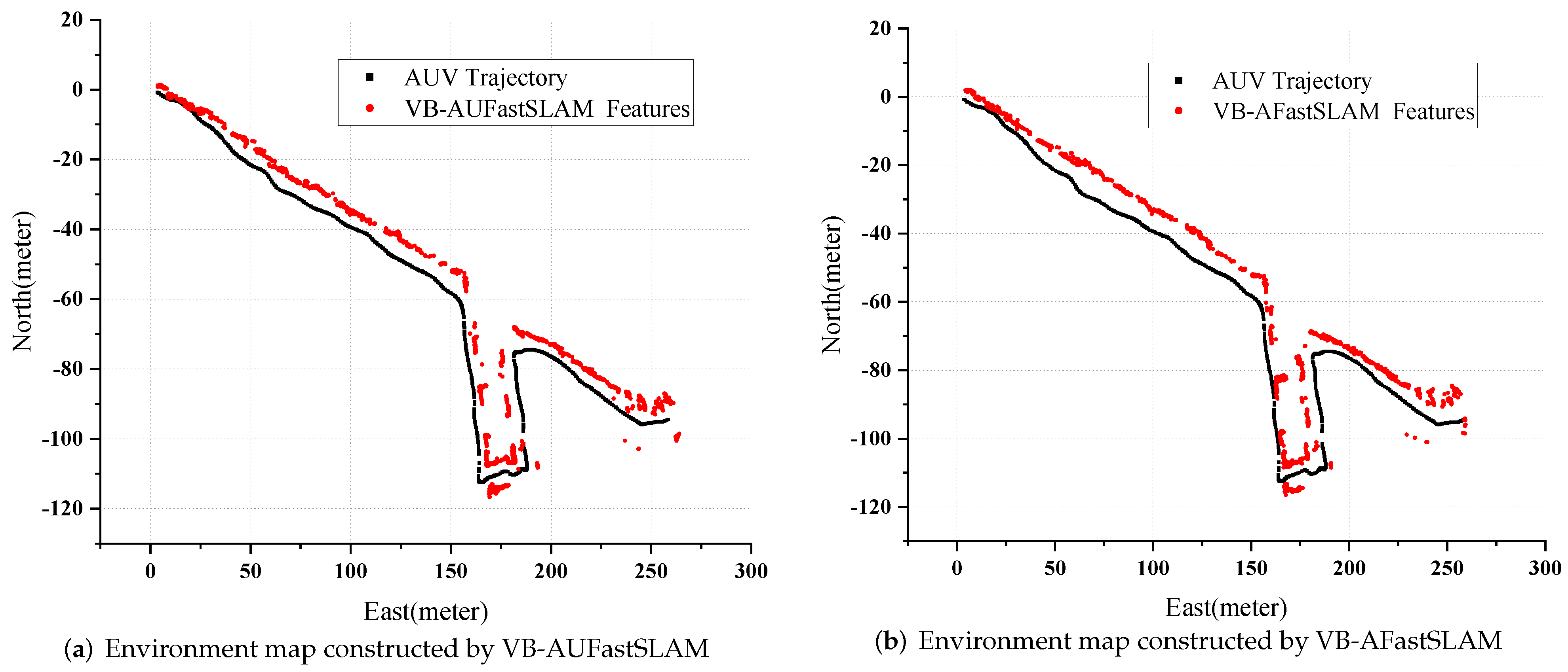
Since the true location of the features are not available, it cannot be quantitatively analyzed. Figure 10a,b are the feature prediction maps of VB-AFastSLAM and VB-AUFastSLAM, respectively. The eastward error (data points 2800 to 3200) of VB-AUFastSLAM in Figure 9b is smaller than that of VB-AFastSLAM. There is some deviation in the map constructed using the VB-AFastSLAM algorithm in Figure 10b. Nevertheless, the maps constructed by the two proposed algorithms generally fit the environmental characteristics.

6. Conclusions and Future Work

This paper proposes the AUV SLAM algorithms that combine the VB method and RBPF-SLAM. The dynamic noise of the sonar is estimated in real-time to improve the accuracy of the algorithm. Based on FastSLAM and UFastSLAM, we propose VB-AFastSLAM and VB-AUFastSLAM, respectively, and verify them in the simulation environment and the real sea trial environment, respectively. In the simulation verification stage, we demonstrated the adaptive ability of the proposed two algorithms to the observation noise by adding time-varying observation noise. At the same time, the large initialization error is verified, and the results show that, as the initialization error gradually increases, the positioning accuracy and feature estimation accuracy both decrease but are still within a reasonable range. Compared with their traditional algorithms, the running time of the two algorithms has increased to a certain extent, but they can meet the real-time performance. In addition, we verified the algorithms in the marine environment with the Sailfish-210 AUV. The Sonar, INS, and DVL data obtained below the water surface are used to locate the robot and map the coastline. The experimental results show that the proposed two algorithms have better localization results than the traditional algorithms, and the map construction is consistent with the actual coastline features.

There are still some challenges in the follow-up work of this paper. First of all, this paper considers the observation noise as white noise and has not solved the problem of colored noise for the time being. In addition, the filter’s performance is somewhat degraded due to the rejection of higher-order components in the linearization of the nonlinear model. Finally, when AUV faces the coastline environment with a single structure and sparse features for a long time, the use of more accurate feature matching techniques is also a key content that needs to be studied.

References

1. Meng, X.; Sun, B.; Zhu, D. Harbour protection: Moving invasion target interception for multi-AUV based on prediction planning interception method. Ocean Eng. 2021, 219, 108268. [Google Scholar] [CrossRef]
2. Paull, L.; Saeedi, S.; Seto, M.; Li, H. AUV Navigation and Localization: A Review. IEEE J. Oceanic Eng. 2014, 39, 131–149. [Google Scholar] [CrossRef]
3. Chen, X.; Huang, J. Combining particle filter algorithm with bio-inspired anemotaxis behavior: A smoke plume tracking method and its robotic experiment validation. Measurement 2020, 154, 107482. [Google Scholar] [CrossRef]
4. Zhao, D.; Liu, X.; Zhao, H.; Wang, C.; Tang, J.; Liu, J.; Shen, C. Seamless integration of polarization compass and inertial navigation data with a self-learning multi-rate residual correction algorithm. Measurement 2021, 170, 108694. [Google Scholar] [CrossRef]
5. Mu, X.; He, B.; Wu, S.; Zhang, X.; Song, Y.; Yan, T. A practical INS/GPS/DVL/PS integrated navigation algorithm and its application on Autonomous Underwater Vehicle. Appl. Ocean Res. 2021, 106, 102441. [Google Scholar] [CrossRef]
6. Zhang, X.; He, B.; Gao, S.; Mu, P.; Xu, J.; Zhai, N. Multiple model AUV navigation methodology with adaptivity and robustness. Ocean Eng. 2022, 254, 111258. [Google Scholar] [CrossRef]
7. Song, J.; Li, W.; Zhu, X.; Dai, Z.; Ran, C. Underwater Adaptive Height-Constraint Algorithm Based on SINS/LBL Tightly Coupled. IEEE Trans. Instrum. Meas. 2022, 71, 1–9. [Google Scholar] [CrossRef]
8. Cadena, C.; Carlone, L.; Carrillo, H.; Latif, Y.; Scaramuzza, D.; Neira, J.; Reid, I.; Leonard, J.J. Past, Present, and Future of Simultaneous Localization and Mapping: Toward the Robust-Perception Age. IEEE Trans. Robot. 2016, 32, 1309–1332. [Google Scholar] [CrossRef] [Green Version]
9. Guo, J.; Jiang, R.; He, B.; Yan, T.; Ge, S.S. General Learning Modeling for AUV Position Tracking. IEEE Intell. Syst. 2020, 35, 28–38. [Google Scholar] [CrossRef]
10. Gu, C.; Cong, Y.; Sun, G. Environment Driven Underwater Camera-IMU Calibration for Monocular Visual-Inertial SLAM. In Proceedings of the 2019 International Conference on Robotics and Automation (ICRA), Montreal, QC, Canada, 20–24 May 2019; pp. 2405–2411. [Google Scholar]
11. Rahman, S.; Li, A.Q.; Rekleitis, I. Sonar Visual Inertial SLAM of Underwater Structures. In Proceedings of the 2018 IEEE International Conference on Robotics and Automation (ICRA), Brisbane, Australia, 21–25 May 2018; pp. 1–7. [Google Scholar]
12. Hess, W.; Kohler, D.; Rapp, H.; Andor, D. Real-time loop closure in 2D LIDAR SLAM. In Proceedings of the 2016 IEEE International Conference on Robotics and Automation (ICRA), Stockholm, Sweden, 16–21 May 2016; pp. 1271–1278. [Google Scholar]
13. Mallios, A.; Ridao, P.; Ribas, D.; Maurelli, F.; Petillot, Y. EKF-SLAM for AUV navigation under probabilistic sonar scan-matching. In Proceedings of the 2010 IEEE/RSJ International Conference on Intelligent Robots and Systems, Taipei, Taiwan, 18–22 October 2010; pp. 4404–4411. [Google Scholar]
14. Simanek, J.; Reinstein, M.; Kubelka, V. Evaluation of the EKF-Based Estimation Architectures for Data Fusion in Mobile Robots. IEEE/ASME Trans. Mechatron. 2015, 20, 985–990. [Google Scholar] [CrossRef]
15. Montemerlo, M.; Thrun, S.; Koller, D.; Wegbreit, B. FastSLAM: A factored solution to the simultaneous localization and mapping problem. In Proceedings of the Eighteenth National Conference on Artificial Intelligence, Edmonton, AB, Canada, 28 July–1 August 2002; pp. 593–598. [Google Scholar]
16. Chen, L.; Yang, A.; Hu, H.; Naeem, W. RBPF-MSIS: Toward Rao-Blackwellized Particle Filter SLAM for Autonomous Underwater Vehicle With Slow Mechanical Scanning Imaging Sonar. IEEE Syst. J. 2020, 14, 3301–3312. [Google Scholar] [CrossRef] [Green Version]
17. Liu, D.; Duan, J.; Shi, H. A Strong Tracking Square Root Central Difference FastSLAM for Unmanned Intelligent Vehicle With Adaptive Partial Systematic Resampling. IEEE Trans. Intell. Transport. Syst. 2016, 17, 3110–3120. [Google Scholar] [CrossRef]
18. Sandoy, S.S.; Matsuda, T.; Maki, T.; Schjolberg, I. Rao-Blackwellized Particle Filter with Grid-Mapping for AUV SLAM Using Forward-Looking Sonar. In Proceedings of the 2018 OCEANS—MTS/IEEE Kobe Techno-Oceans (OTO), Kobe, Japan, 28–31 May 2018; pp. 1–9. [Google Scholar]
19. Kim, C.; Sakthivel, R.; Chung, W.K. Unscented FastSLAM: A Robust and Efficient Solution to the SLAM Problem. IEEE Trans. Robot. 2008, 24, 808–820. [Google Scholar] [CrossRef]
20. Nguyen, H.K.; Wongsaisuwan, M. A study on Unscented SLAM with path planning algorithm integration. In Proceedings of the 2014 11th International Conference on Electrical Engineering/Electronics, Computer, Telecommunications and Information Technology (ECTI-CON), Nakhon Ratchasima, Thailand, 14–17 May 2014; pp. 1–5. [Google Scholar]
21. Tang, M.; Chen, Z.; Yin, F. An improved H-infinity unscented FastSLAM with adaptive genetic resampling. Robot. Auton. Syst. 2020, 134, 103661. [Google Scholar] [CrossRef]
22. Lin, M.; Yang, C.; Li, D. An Improved Transformed Unscented FastSLAM With Adaptive Genetic Resampling. IEEE Trans. Ind. Electron. 2019, 66, 3583–3594. [Google Scholar] [CrossRef]
23. Yin, S.; Zhu, X. Intelligent Particle Filter and Its Application on Fault Detection of Nonlinear System. IEEE Trans. Ind. Electron. 2015, 62, 3852–3861. [Google Scholar] [CrossRef]
24. Cui, J.; Feng, D.; Li, Y.; Tian, Q. Research on simultaneous localization and mapping for AUV by an improved method: Variance reduction FastSLAM with simulated annealing. Def. Technol. 2020, 16, 651–661. [Google Scholar] [CrossRef]
25. Poulose, A.; Han, D.S. Hybrid Indoor Localization Using IMU Sensors and Smartphone Camera. Sensors 2019, 19, 5084. [Google Scholar] [CrossRef] [Green Version]
26. Lin, M.; Yang, C.; Li, D.; Zhou, G. Intelligent Filter-Based SLAM for Mobile Robots with Improved Localization Performance. IEEE Access 2019, 7, 113284–113297. [Google Scholar] [CrossRef]
27. Wang, J.; Zhang, T.; Jin, B.; Zhu, Y.; Tong, J. Student’s t-Based Robust Kalman Filter for a SINS/USBL Integration Navigation Strategy. IEEE Sens. J. 2020, 20, 5540–5553. [Google Scholar] [CrossRef]
28. Zhang, T.; Wang, J.; Zhang, L.; Guo, L. A Student’s T-Based Measurement Uncertainty Filter for SINS/USBL Tightly Integration Navigation System. IEEE Trans. Veh. Technol. 2021, 70, 8627–8638. [Google Scholar] [CrossRef]
29. Sarkka, S.; Nummenmaa, A. Recursive Noise Adaptive Kalman Filtering by Variational Bayesian Approximations. IEEE Trans. Automat. Control 2009, 54, 596–600. [Google Scholar] [CrossRef]
30. Bailey, T.; Durrant-Whyte, H. Simultaneous localization and mapping (SLAM): Part II. IEEE Robot. Automat. Mag. 2006, 13, 108–117. [Google Scholar] [CrossRef]
Figure 1. The Sailfish-210 AUV.
Jmse 10 01563 g001
Figure 2. Navigation coordinate system of Sailfish AUV.
Jmse 10 01563 g002
Figure 3. Simulation Environment.
Jmse 10 01563 g003
Figure 4. Dynamic observation noise is set to n = 3; p = 0.2.
Jmse 10 01563 g004
Figure 5. n = 2; p = 0.3, algorithms error comparison.
Jmse 10 01563 g005
Figure 6. Comparison of Neff with different observation noise.
Jmse 10 01563 g006
Figure 7. AUV trajectory.
Jmse 10 01563 g007
Figure 8. Sailfish-210 during the mission.
Jmse 10 01563 g008
Figure 9. Comparison chart of sea trial trajectory and error comparison of four algorithms.
Jmse 10 01563 g009
Figure 10. The results of the proposed two algorithms for building the map.
Jmse 10 01563 g010