URANS Calculation of Ship Heave and Pitch Motions in Marine Simulator Based on Overset Mesh

Abstract

So as to improve the reliability and accuracy of marine simulators, it is essential to predict ship heave and pitch motions in regular waves. The motions of two ships, the international standard model KVLCC2 and the first training ship, “Yukun”, of Dalian Maritime University, are simulated using a three-dimensional (3D) numerical wave tank based on the Unsteady Reynolds Averaged Navier–Stokes (URANS) equations. The free surface is captured by the volume of fluid (VOF) method, and an SST k-ω turbulence model is used to describe the turbulence flow. The numerical model is first validated for the standard KVLCC2 at three different speeds through a comparison with the published experimental data and the potential flow results. Then, numerical simulation is performed for the motion of the ship Yukun with different speeds under various sea conditions. The heave amplitude of the hull changes with the increase in the wavelength when the maximum value is reached. Upon comparing the RAOs of ship motions under different wave steepness conditions, it is apparent that the heave and pitch motions of ships nonlinearly decrease with an increase in wave steepness. The results were added to the database of the marine simulator to further improve the accuracy and realism of the simulator.

1. Introduction

A marine simulator (Figure 1 and Figure 2) is an efficient and low-cost simulation training platform for ship pilots based on virtual reality technology [1]. The mathematical model of ship motions directly affects the quality of the marine simulator. Under the action of waves, it is inevitable for ships to heave, pitch and sway from different angles. Therefore, it is significant to study a ship’s heave and pitch motion in waves and add the ship motion’s effects on behavioral authenticity to the simulator to improve its accuracy. Different methods have been used to establish the mathematical model (of ship motion mathematical model) in marine simulators to date. Potential flow theory is the most popular. Ren [2] has studied the heave and pitch motion of high-speed ships under top waves based on the approximate calculation formula. Zhang [3] conducted relevant studies based on the Froude–Krylov hypothesis, and Zhang [4] employed the multi-coefficient conformal transformation method based on the two-dimensional linear potential flow theory. Although the heave and pitch of ships in waves are considered within the frame of the marine simulator, the ship motions are not well resolved by the adopted potential flow simulations due to their limitations. The adopted potential flow theory does not consider the viscous effect of water.

An alternative choice is CFD solvers. The research results regarding the heave and pitch motions of ships in waves are quite abundant in the field of ship and ocean engineering. Carrica [5] examined the motions of DTMB-5512 at different speeds under the condition of head waves using overset mesh technology. Kim [6,7] carried out numerical simulations against the head sea by establishing a numerical wave tank and combining this with dynamic mesh technology. Using the overset mesh technology, Carrica directly simulated the KCS in calm water and head wave (wave direction angle β = 180°). Although this is more resource-intensive, CFD simulation provides more flow details [8]. Muscar used the overset mesh technology to simulate flow detail further [9]. Gaggero developed a program to simulate KCS in calm water [10]. Shen calculated and analyzed the motions of Wigley-III and KCS at different speeds and wavelengths in the head wave using the dynamic mesh technique [11,12]. Xu established a numerical wave tank and combined this with overset meshes to evaluate the motions of DTMB-5512 in the head sea ahead navigation [13]. Cao established a 3D numerical wave tank and combined it with overset mesh technology to disclose the motions of ships under different wavelengths and wave heights under head wave conditions [14]. At the moment, the mathematical models of heave and pitch motion in navigation simulation are mainly focused on empirical formulae and potential flow theory. Traditional empirical formulas will not be able to provide more accurate results as ships expand and diversify. The potential flow hypothesis was developed by ignoring water viscosity. It is limited in its ability to obtain more accurate flow field information. The viscous flow theory will be used in this study to obtain accurate process and flow field information of the entire dynamic change process of the ship’s heave and pitch motion when encountering waves. According to the theory of viscous flow, these results focused on the heave and pitch motions of ships with different wavelengths, velocities and wave steepness in the case of head wave navigation, and laid a solid theoretical foundation for research into ship heave and pitch motions. However, the CFD method still faces great challenges when dealing with mesh deformation on the condition of ships moving over a large range and complex ship models owing to its single research condition (especially for the angle of wave condition). In addition, the marine simulator focuses on the whole process, from the beginning to the stability of ship motions in the wave. In order to increase the realism of the marine simulator’s behavior, the viscous flow theory is coupled with it, and the commercial program STAR-CCM+ is used to numerically model the ship’s heave and pitch motion during the whole dynamic transition process from an unstable state to steady state.

A 3D numerical wave tank is built in this work to produce, propagate, and remove waves. A mathematical model of ship heave and pitch motions is built to expand the existing ship model in the marine simulator under various sea conditions. Overset mesh technology is used to capture the ship’s motions. The numerical model is first validated for the standard KVLCC2 at different speeds 3(0 kn, 12 kn, and 15 kn) through a comparison with the published experimental data and the potential flow results. The heave and pitch motions of the ship under different speeds, wavelengths, and wave steepness are simulated and analyzed. Further investigation is carried out for the first training ship, “Yukun”, of Dalian Maritime University. The heave and pitch motions of the ship at a speed of 16.7 kn, angle 0°, 45°, 90°, 135°, and 180°, wave height (H)/Wavelength(λ) 2/25, 2/35, 2/50, 2/80, and 2/100 are calculated. The results are added to the database of the marine simulator to further improve the accuracy and realism of the simulator.

2. Materials and Methods

2.1. Fluid Governing Equation

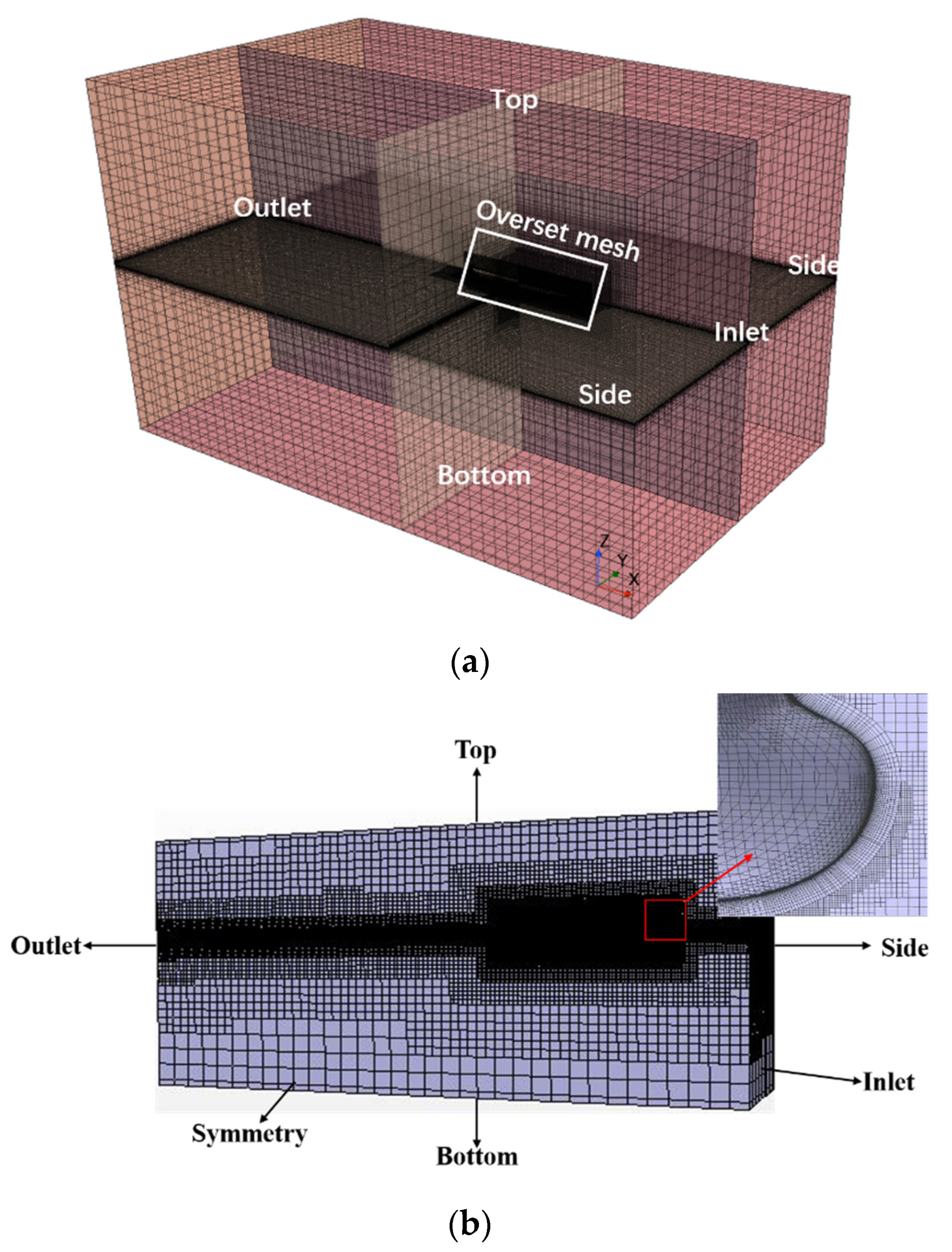
The governing Unsteady Reynolds Averaged Navier–Stokes equations [15] consist of continuity and momentum equations, in conjunction with the closure model chosen as the SST k-ω turbulence model. More specifically,

$$\nabla ·u=0,$$

(1)

$$\frac{\partial \rho u}{\partial t}+\nabla ·\left(\rho uu\right)=-\nabla p+\nabla ·\left(\mu \nabla u\right)+g\rho ,$$

(2)

where $u$ is the velocity vector with components of the velocity (u, v, w) in the x-, y-, and z-direction, respectively, and t, p, $\rho$, $\mu$, and g are the time, the pressure, the density, the dynamic viscosity coefficient, and gravitational acceleration, respectively.

Moreover, the turbulence model used in the present work is defined by,

$$\frac{\partial }{\partial t}\left(\rho k\right)+\nabla \cdot \left(\rho k\overline{v}\right)=\nabla \cdot \left[\left(\mu +{\sigma }_k{\mu }_t\right)\nabla k\right]+P_k-\rho {\beta }^{*}{f}_{{\beta }^{*}}\left(\omega k-{\omega }_0{k}_0\right)+S_k$$

(3)

$$\frac{\partial }{\partial t}\left(\rho \omega \right)+\nabla \cdot \left(\rho \omega \overline{v}\right)=\nabla \cdot \left[\left(\mu +{\sigma }_{\omega }{\mu }_t\right)\nabla \omega \right]+P_{\omega }-\rho \beta f_{\beta }\left({\omega }^2-{\omega }_0^2\right)+S_{\omega }$$

(4)

where $\overline{v}$ is the average velocity. ${\sigma }_k$, ${\sigma }_{\omega }$, and ${\beta }^{*}$ are the model coefficient. $P_k$ and $P_{\omega }$ are the result term. $f_{{\beta }^{*}}$is the free shear correction factor. $S_k$and $S_{\omega }$are the source term. $k_0$and ${\omega }_0$ are the environmental turbulence values to prevent turbulence attenuation and $f_{\beta }$is the eddy current extension correction factor.

At present, there are many methods of capturing the free surface, such as the Level-Set function method, MAC method, and VOF method. In this study, a simple and stable VOF method was adopted to capture the fluctuations in the free surface [16]. The air and water are considered as two incompressible, isothermal, and immiscible fluids.

$$\frac{\partial \alpha }{\partial t}+\nabla ·\left(u\alpha \right)=0,$$

(5)

where $\alpha$ is the volume fraction, which is defined as the relative proportion of water in each cell. If $\alpha =1$, the cell is full of water and if $\alpha =0$, the cell is full of air, and in any other case, the cell contains the interface between the two phases.

In the numerical calculations in this study, the finite volume method was used to discretize the governing equations, the second-order upwind scheme was applied to the convection term, and the central difference scheme was used for the diffusion term. The semi-implicit method for pressure-linked equations (SIMPLE) algorithm was employed to separate the solution. In considering the influence of gravity, the overset mesh method was opted to solve the discrete algebraic equations.

2.2. Overset Mesh

The main idea of overset mesh technology is to create multiple sets of overset meshes, search the boundary of the overset area in iterative calculations, and identify the real physical boundaries for calculation. Compared with traditional mesh, the most prominent advantage of overset mesh is that it can capture a large range of object motions without deforming the mesh during the process. As shown in Figure 3, information was transmitted between the background area and the overset area through the interface.

The overset mesh method is used to separate the mesh around the moving object. The mesh can be either structured or unstructured, and there are overset parts between multiple nested meshes. The key to overset mesh method is to establish domain connectivity information (DCI) and transfer information between meshes. DCI is mainly composed of element information and interpolation weight coefficient.

$${\varphi }_l={{\displaystyle \sum }}_{i=1}^n{\omega }_i\cdot {\varphi }_i$$

(6)

where $\varphi$is the arbitrary flow field information, such as velocity, pressure, etc. ${\varphi }_{i }$ is the value of interpolation boundary element. ${\varphi }_{i }$ is the flow field information value of the $i$ -th contribution unit. ${\omega }_i$ is the interpolation weight coefficient of the$i$-th contribution unit, which needs dimensionless processing and meets the requirements ${{\displaystyle \sum }}_{i=1}^n{\omega }_i=1$.

As shown in Figure 4, the simulation was carried out with a set of overset meshes. The background mesh size was set to be larger and the overset mesh size to be smaller to reduce the number of meshes, and a mesh transition area was set up around the overset area to complete the transition from the larger background mesh to the smaller overset mesh at an appropriate rate. Within the overset mesh area, the background mesh size was larger than the overset mesh size. Three sets of mesh densification were set up. One was for the surface mesh of the ship, which was mostly used to alter the Y+ value by adjusting the thickness of the first layer of mesh. The other two were used to encrypt the bow and stern body meshes, respectively. The operation’s primary goal was to clearly examine the flow field changes in the bow and stern, particularly in relation to the wave condition on the deck. Finally, the free surface was encrypted in order to detect changes in the flow field surrounding the ship precisely.

In general, when using overset meshes, attention should be paid to the following issues. The size of the interface between the background mesh and the overset domain mesh should be consistent as far as possible. The mesh at the interface should satisfy at least two layers. The appropriate method should be selected for the mesh interpolation at the interface. It is recommended to use the linear interpolation method.

As shown in Figure 5, the origin of the coordinate system was at the ship’s center of mass. The axis pointed to the bow of the ship, the axis pointed to the port side of the ship, and the axis pointed to the vertical upward. The motions around the three directions were surge, swing, and heave, respectively, and the rotation motions around the three directions were roll, pitch, and yaw, which was the wave angle. When β = 180°, the ship sailed in head wave; when β = 90°, the port side of the ship suffered from the transverse wave; when β = 0°, the ship followed the waves.

As shown in Figure 6, the setting size of the 3D wave numerical tank in this study varies with the wavelength: the background area is set as the front end of the ship 1λ, the rear end of the ship 4λ (including 1.5λ wave damping area), the water depth is 2 Length between perpendiculars $\left(L_{pp}\right)$, the top of the ship is 1$L_{pp}$, and the left and right ends of the ship are 2$L_{pp}$, respectively. The overset area is set to be 1.5$L_{pp}$, 2D in height and 2B in width.

3. Results

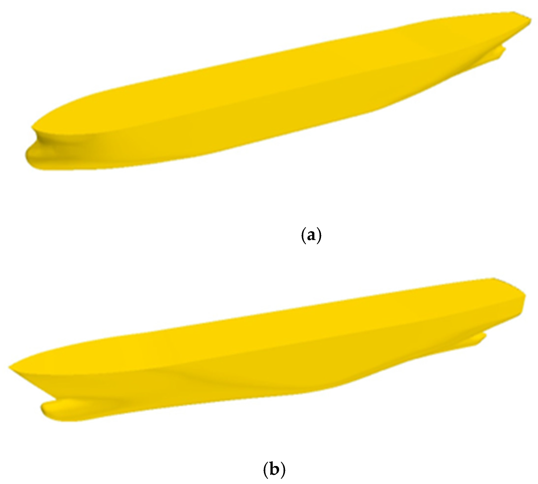
3.1. Test Ship and Numerical Setup

The research objects of this study are KVLCC2 and “Yukun”. Two ship models are shown in Figure 7. The geometric parameters are shown in

Table 1. Main particulars of KVLCC2 hull.

Particulars	Full Scale	Model Scale
${\mathit{L}}_{\mathit{p}\mathit{p}}$(m)	320	4
B (m)	58	0.725
D (m)	20.8	0.260
$\mathbf{\nabla }$ (m3)	312,622	0.6106
LCG (%)	3.48	3.48
VOG(m)	18.56	0.232
CB	0.8098	0.8098

and

Table 2. Main particulars of “Yukun” hull.

Particulars	Full Scale	Model Scale
${\mathit{L}}_{\mathit{p}\mathit{p}}$ (m)	105	2.1
B (m)	18	0.36
D (m)	5.4	0.108
$\mathbf{\nabla }$ (m3)	5711	0.04569
K (m)	26.25	1.575
CB	0.5596	0.5596

.

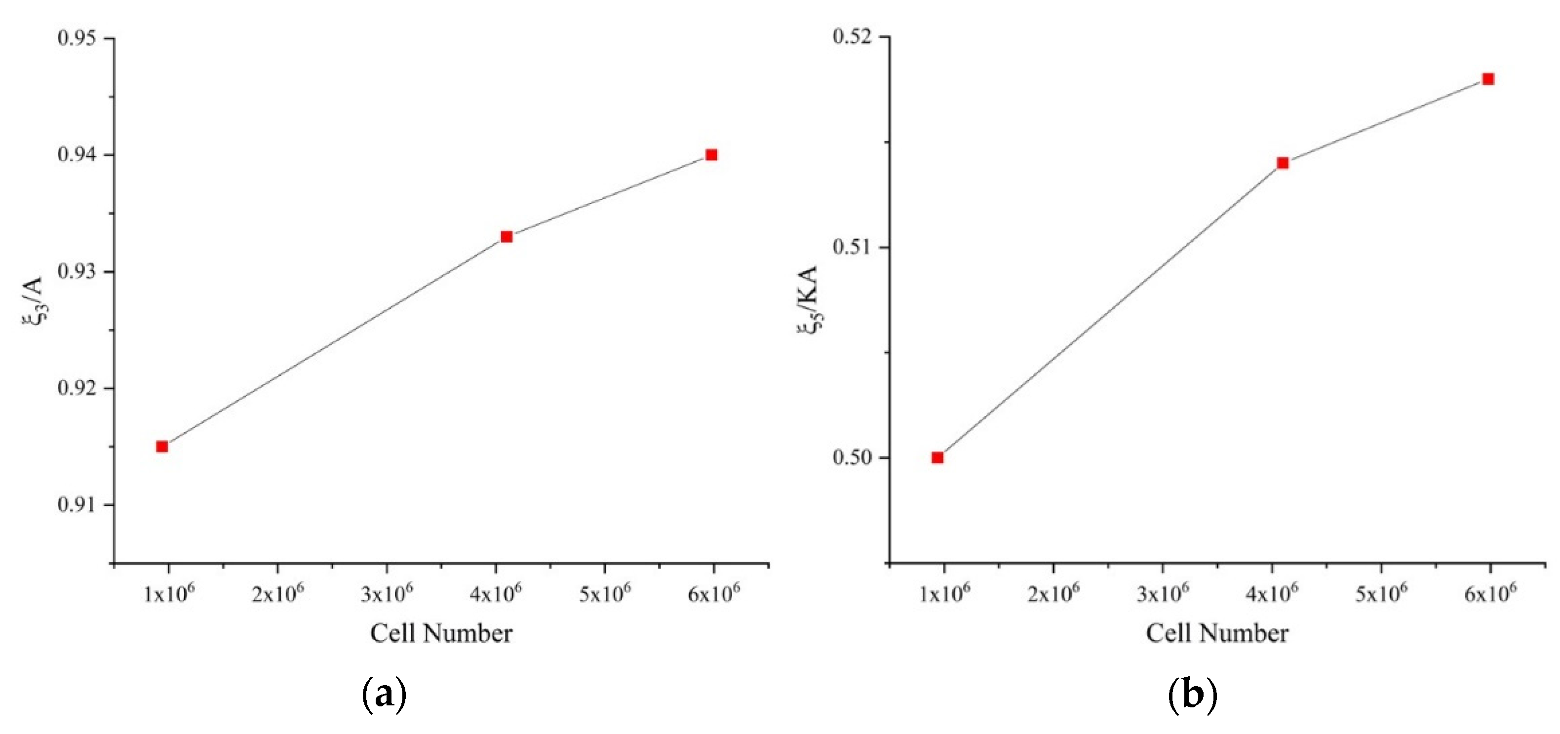
3.2. Mesh Generation and Mesh Independence Study

As shown in Figure 8a, the full calculation domain was mainly used to calculate the ship’s angle of the wave at 45°, 90°, and 135°. At large, the external conditions (inlet, outlet, and side) include the bottom of the tank, the top of the tank, and the overset area. Specific boundary conditions were set as follows. The background area is set as the front end of the ship 1λ, the rear end of the ship 4λ, the water depth is 2$L_{pp}$, the top of the ship is 1$L_{pp}$, and the left and right ends of the ship are 2$L_{pp}$, respectively. The overset area is set to be 1.5$L_{pp}$, 2D in height and 2B in width. External conditions were set as velocity inlet, including fluid velocity, water volume fraction, turbulence intensity, turbulence viscosity ratio, and VOF wave force boundary options. The bottom and side were set as walls, including mixed wall function and shear stress. The tank top was set as a pressure outlet, including static pressure, volume fraction, turbulence intensity, turbulent viscosity ratio, and VOF wave force boundary options. The overset boundary was set as the overset mesh type. The hull was set as a wall, including mixed wall function and shear stress. Figure 8b is a semi-computational domain. The background area is set as the front end of the ship 1λ, the rear end of the ship 4λ, the water depth is 2$L_{pp}$, the top of the ship is 1$L_{pp}$, and the left end of the ship are 2$L_{pp}$, respectively. The overset area is set to be 1.5$L_{pp}$, 2D in height, and B in width. It mainly calculated the angle of the wave at 0° and 180° and what is needed to modify the outlet as the pressure outlet and the top of the tank as the velocity inlet.

The grid division technique densifies the critical areas of the ship, including the free liquid surface and surrounding the ship’s hull, to more realistically recreate the ship’s heave and pitch motions in waves. Simultaneously, the grid with a bigger grid foundation size is used in the far field region to conserve computing resources, and the transition from the background area to the overlapping area is seamless. The grid foundation is 0.2 m in size. Pay careful attention to the thickness of the first layer of the boundary layer grid, which is controlled by Y + and is about 50.

As this study mainly investigates the motions of ships in waves, wave mesh creation should be the primary focus. To accurately capture the free surface, enough meshes should be placed along the free surface in the vertical direction. To ensure the accurate transmission of information between the mesh in the background domain and the overset domain, the mesh size of the boundary mesh in the aforementioned two domains should be consistent. In order to obtain accurate flow field information around the hull and reduce the amount of calculation needed, the mesh density around the hull should be appropriately increased, and the mesh size of the surrounding flow field should be increased. In this study, the hull wall was set as 7-layer boundary layer mesh, and Y+ was taken to be 50.

So as to facilitate the comparison between the experimental data and other references, the numerical results need to be dimensionless. The response amplitude operator (RAO) formula of heave and pitch is shown in Equation (7).

$$H_{RAO}=\frac{{\xi }_3}{A}, P_{RAO}=\frac{{\xi }_5}{kA}$$

(7)

where $A$is the amplitude of encountering wave. ${\xi }_3$and ${\xi }_{5 }$ are the amplitude of heave and pitch motions respectively and $k$is the wave number.

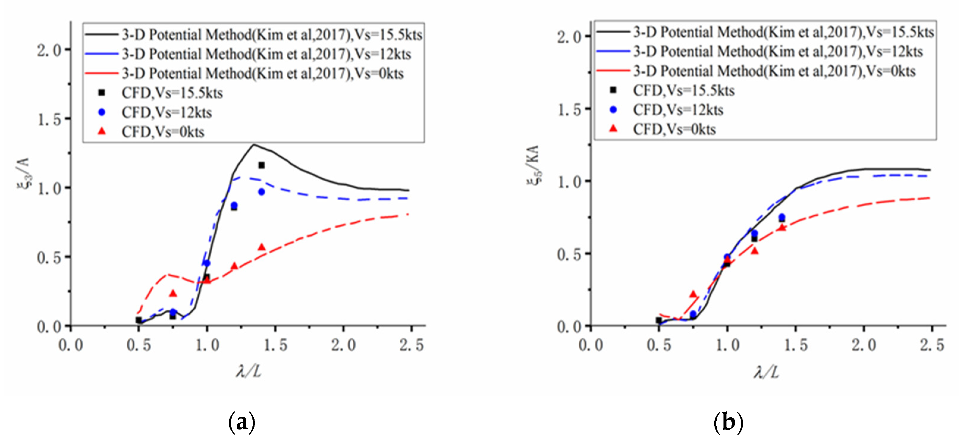
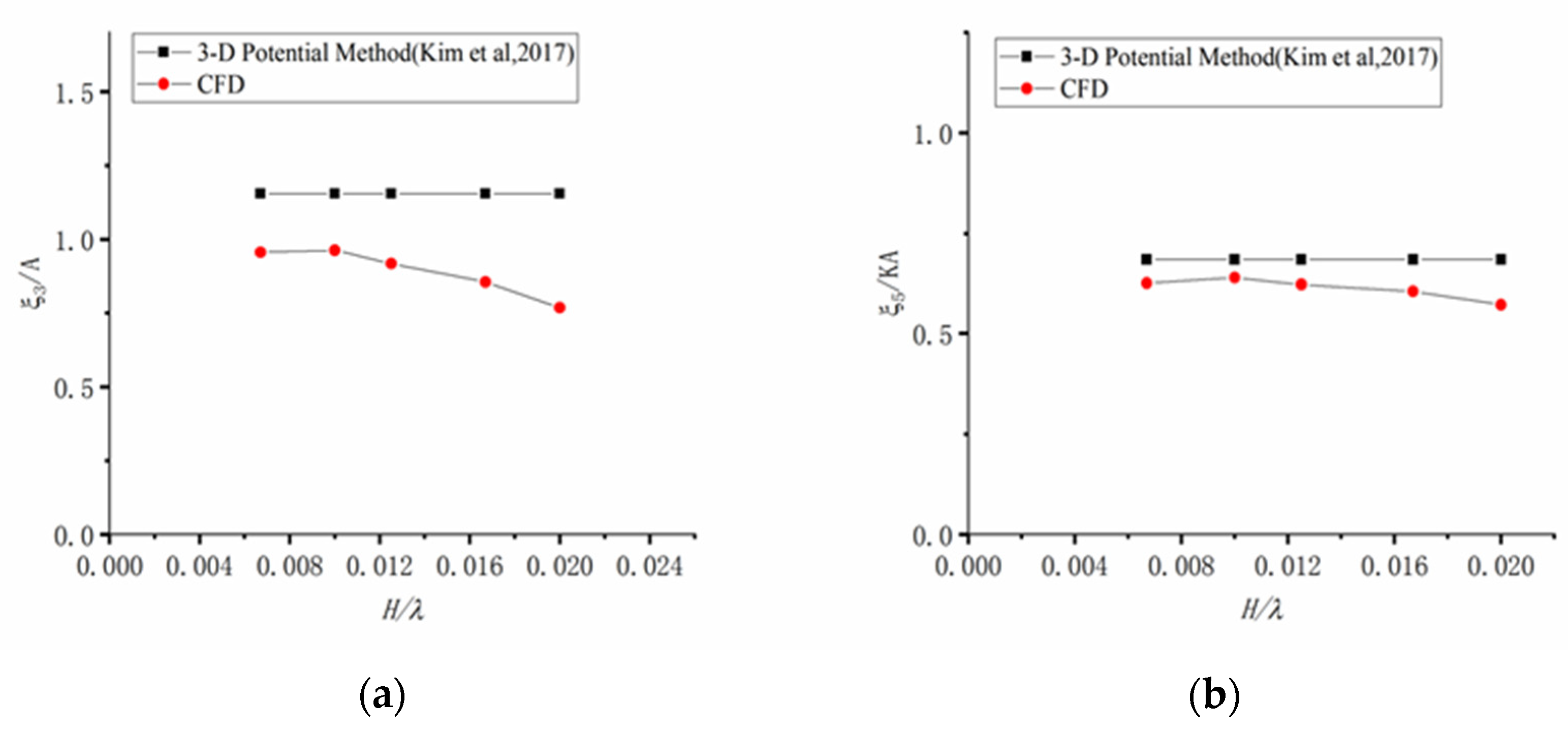
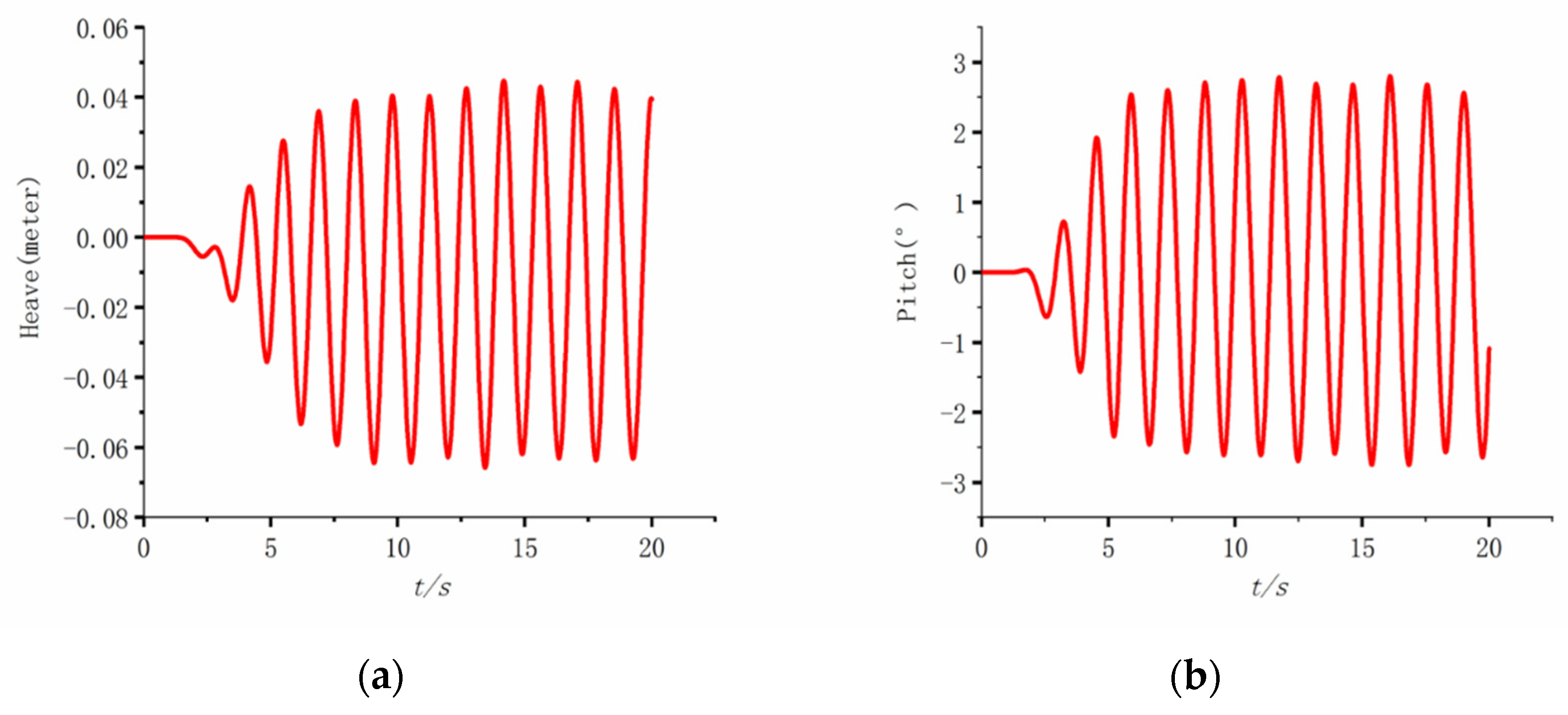
3.3. Numerical Simulation of KVLCC2

This section mainly deals with the heave and pitch motions of KVLCC2 at different speeds, wavelengths, and wave heights. The number of mesh is about 1.8–2.2 million. Before the numerical simulation of KVLCC2, mesh convergence tests are carried out under the conditions of V = 15.5 knots ($Fn$= 0.142) and λ/$L_{pp}$= 1. Specific parameters are shown in

Table 3. Test cases for mesh convergence (λ/$L_{pp}$= 1, $H$/λ = 1/60, V = 15.5 knots).

Case (No.)	Mesh	Mesh Number	$∆z/∆x$	$T_e/∆t$
CKC	Coarse	0.8 million	1/8	180
CKB	Base	2.1 million	1/8	256
CKF	Fine	4.1 million	1/8	340

. CFD calculation time for coarse mesh, base mesh, and fine mesh was 1 day, 2–3 days, and 3–4 days (24CPUs @ 2 GHz), respectively.

A reasonable mesh density implies that both numerical accuracy and computing efficiency must be considered. For that purpose, three types of meshes with varying densities are constructed by varying the mesh size of the free surface while keeping the mesh of the ship entry constant. The fundamental size ratio between neighboring density grids is $\sqrt{2}$, according to ITTC’s requirements for the application of CFD in ships [17]. The RAO of heave and pitch movements with three mesh numbers is shown in Figure 9. Figure 10 shows the heave and pitch time history of case CKB. Compared with the experimental results in reference [16], we can see that the heave and pitch errors are 9.1% and 2.3%, respectively, in case CKC (grid number is 2.1 million), and are 8.8% and 1.9%, respectively, in case CKF (grid number is 4.1 million). From the overall view of the three groups of meshes, 2.1 million meshes can effectively improve computational efficiency while meeting the accuracy. In the study of the KVLCC2 ship model sailing in the head wave, the CKB mesh segmentation method is adopted, and the case simulation, as shown in

Table 4. Test Cases of KVLCC2.

Case (No.)	V [Knots]	$\mathbf{Wavelength}$ $(\mathit{\lambda }/{\mathit{L}}_{\mathit{p}\mathit{p}})$	$\mathbf{Wave} \mathbf{Height}$ $\left(\mathit{H}\right)\left[\mathbf{m}\right]$	$\mathbf{Wave} \mathbf{Steepness}$ $(\mathit{H}/\mathit{\lambda })$
CK1	15.5	0.5	2.67	1/60
CK2	15.5	0.75	4	1/60
CKB	15.5	1	5.33	1/60
CK4	15.5	1.2	6.4	1/60
CK5	15.5	1.4	6.4	1/60
CK6	12	0.75	4	1/60
CK7	12	1	5.33	1/60
CK8	12	1.2	6.4	1/60
CK9	12	1.4	7.47	1/60
CK10	0	0.75	4	1/60
CK11	0	1	5.33	1/60
CK12	0	1.2	6.4	1/60
CK13	0	1.4	7.47	1/60
CK14	15.5	1.2	2.56	1/150
CK15	15.5	1.2	3.84	1/100
CK16	15.5	1.2	4.8	1/80
CK17	15.5	1.2	6.4	1/60
CK18	15.5	1.2	7.68	1/50

below, is carried out.

Comparing the RAO of heave and pitch with experimental data [18,19] and potential flow theory results [6,7], as shown in Figure 11, with the increase in $\lambda$/$L_{pp}$, the amplitude of heave and pitch also increases, and the heave reaches its maximum value near $\lambda$/$L_{pp}$ = 1.4. The heave motion of the resonance period is slightly underestimated by the CFD simulation when the resonance period meets 1 < $\lambda$/$L_{pp}$ < 1.4. Regarding pitch motion, the CFD results agree with the experimental results. In general, when V = 15.5 knots, the CFD results are consistent with the experimental results and potential flow theory results. Under the long wave conditions, when the wave height near the middle of the ship is 0, the distribution of the wave height along the length of the ship is monotonous (increasing or decreasing), and the trim angle reaches the maximum or minimum values. At this time, the buoyancy of the bow and stern changes inversely with the trim of the ship, which compensates for each other, so the heave motion is in the equilibrium position. In addition, on the condition that the wave crest or trough is near the middle of the ship, the buoyancy of the bow and stern are the same, and the ship is in positive buoyancy. This means that the total buoyancy reaches the maximum or minimum, and the hull needs to balance the gravity by floating or sinking [20]. Overall, both the results of the numerical simulation and the experiment show that the ship is in the state of following the wave under long wave conditions, which is consistent with the real physical situation.

To consider slow sailing or the actual speed of the ship, two more cases with V = 12 knots and V = 0 knots are investigated and compared with the results of the potential flow theory. Figure 12 shows that the potential flow theory and CFD results are quite different near the resonance period. When V = 12 knots, the heave amplitude increases with the increase in $\lambda$/$L_{pp}$, and reaches the maximum at 1.2 < $\lambda$/$L_{pp}$ < 1.3. However, there is a large difference between the CFD calculation results of the resonance period part and the potential flow theory calculation results; the calculation results of other parts of CFD in heave motion are in good agreement with the potential flow theory results, and the pitch motion also increases with the increase in $\lambda$/$L_{pp}$. The overall trend is in good agreement with the potential flow theory results. In general, when V = 15.5 knots and 12 knots, compared with the CFD results, the response with potential flow theory in heave and pitch motions near the resonance period exceeds the CFD results; however, in the simulation of V = 0 knots, the heave and pitch responses near the resonance period are in fine agreement with the CFD results.

It can be observed from Figure 13 that by comparing the RAO of heave and pitch under different wave steepness conditions, the heave and pitch motions of ships, especially the heave motion calculated by CFD, decrease nonlinearly with the increase in wave steepness.

The purpose of the marine simulator is to allow the crew to experience the whole process of ship movement, with the goal of achieving authenticity. As a result, the marine simulator concentrates on the entire process of ship movement, from beginning to stability. Therefore, the RAO is calculated and compared with the experimental data and the potential flow theory results, which proves that the method used in this study is accurate and reliable in the calculation of heave and pitch [21]. Finally, whole-time history data of CFD calculation are combined in the marine simulator. Therefore, as shown in Figure 14, only one case in Table 4 is selected. For example, KVLCC2 chooses a time period from 0 s to 20 s in V = 15.5 knots. The marine simulator focuses on the whole process, from 0 s to stability.

Broadly speaking, the heave and pitch of KVLCC2 in the head wave were simulated under different speeds, wavelengths, and wave steepness. The CFD results are in good agreement with the experimental results and potential flow theory results, especially for those near the resonance period, which can effectively avoid the changes in heave amplitude caused by common vibration.

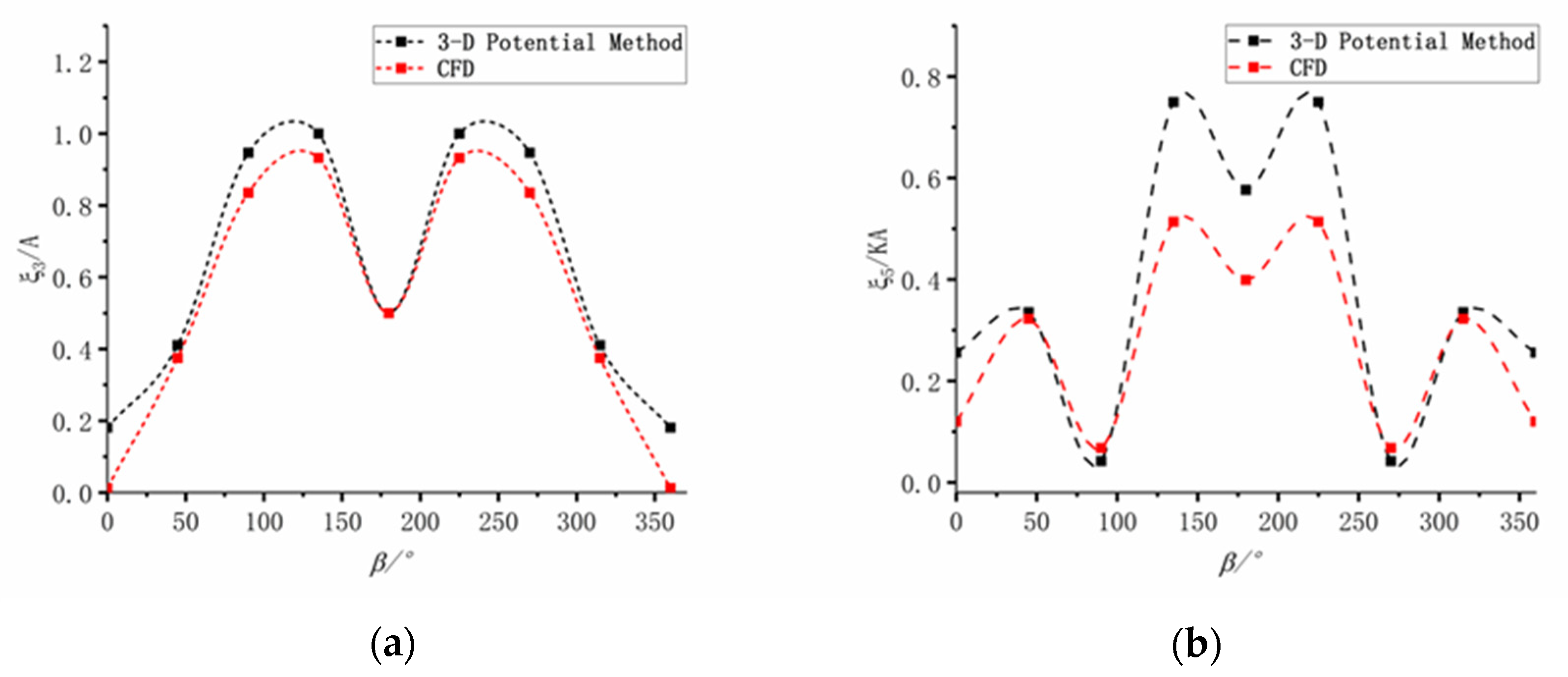
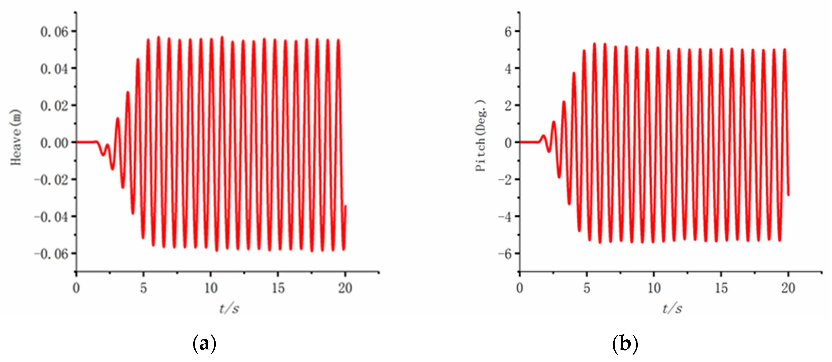
3.4. Numerical Simulation of Yukun

In this section, the angle of the wave of “Yukun” with a large angle is simulated. The mesh number is about 2 million (head wave) and 4.1 million (large angle of wave). Before the simulation, the mesh convergence is analyzed.

Table 5. Test Cases of Yukun.

Case (No.)	Mesh	Mesh Number	$\mathbf{∆}\mathit{z}/\mathbf{∆}\mathit{x}$	${\mathit{T}}_{\mathit{e}}/\mathbf{∆}\mathit{t}$
CYC	Coarse	0.96 million	1/8	180
CYB	Base	4.1 million	1/8	256
CYF	Fine	5.98 million	1/8	340

shows the convergence test conditions of “Yukun” mesh. CFD calculation time for coarse mesh, base mesh, and fine mesh was 1 day, 3–4 days, and 5–6 days (24CPUs @ 2 GHz), respectively.

Similar to KVLCC2, three groups of mesh are designed by changing the mesh size of the free surface. The RAO of heave and pitch motions under three mesh numbers are shown in Figure 15 and Figure 16, showing the heave and pitch time history of case CYB. Error is defined as the relative error between adjacent density meshes based on the coarse mesh calculation results. By comparing the RAO of heave and pitch, CYB is 4.1 million mesh, the error of heave and pitch relative to CYC is 1.97% and 2.8%, and CYF is 5.98 million mesh. Compared with CYC, the heave and pitch errors are 2.73% and 3.6%, respectively. As a whole, the accuracy of 4.1 million meshes can effectively improve computational efficiency. The CYB mesh segmentation method is adopted to study the navigation of the “Yukun” ship model in large angle waves. The simulation conditions are shown in

Table 6. Test Cases of “Yukun”.

Case (No.)	V [knots]	Wave Angle [°]	$\mathbf{Wavelength}$ $(\mathit{\lambda }/{\mathit{L}}_{\mathit{p}\mathit{p}})$	$\mathbf{Wave} \mathbf{Height}$ $\left(\mathit{H}\right)$ $\left[\mathbf{m}\right]$	$\mathbf{Wave} \mathbf{Steepness}$ $(\mathit{H}/\mathit{\lambda })$
CY1	16.7	0	1	0.12	2/35
CY2	16.7	45	1	0.12	2/35
CY3	16.7	90	1	0.12	2/35
CY4	16.7	135	1	0.12	2/35
CY5	16.7	180	1	0.12	2/35
CY6	16.7	135	1	0.042	2/100
CY7	16.7	135	1	0.0525	2/80
CY8	16.7	135	1	0.084	2/50
CY9	16.7	135	1	0.168	2/25

. The “Yukun” potential flow results are from reference [22].

Figure 17 shows that the amplitude of ship motions is symmetrical with respect to the wave angle at β = 180°. In terms of heave motion, when the wave angle is 90° ≤ β < 140°, the heave amplitude of the ship slowly increases with the increase in the wave angle. When the wave angle is 45° ≤ β < 130°, the heave amplitude rapidly increases, and when the wave angle is 135° ≤ β ≤ 180°, the heave amplitude rapidly decreases. Meanwhile, the maximum amplitude of heave motion is located at the wave angle β = 135°, and the minimum amplitude of heave motion is at the position of wave angle β = 0°. In terms of pitch motion, when the wave angle is 0° ≤ β < 45°, the amplitude of pitching motion increases slowly with the increase in wave angle and rapidly decreases when the wave angle is 45° ≤ β ≤ 90°. The minimum value is obtained at 90°. After that, the pitch amplitude rapidly increases when the angle is 90° ≤ β < 140°, and the pitch amplitude reaches the maximum at about 140°. Additionally, the pitch amplitude slowly decreases at 140° ≤ β < 180°. Generally speaking, the potential flow theory results were larger than the CFD results in terms of heave and pitch motions, and the deviation between potential flow theory and CFD results reached the maximum under β = 0°. The results reveal that the pitch amplitude potential flow theory results showed the largest deviation compared with the CFD results at β = 135°.

As shown in Figure 18, for example, the heave and pitch time histories of the “Yukun” ship at V = 16.7 knots and β = 135° were selected to explain the process from 0 s to 20 s. The marine simulator pays more attention to the whole process, from 0 s to 20 s. Figure 19 shows that, by comparing the RAO of heave and pitch under different wave steepness conditions, the heave and pitch motions of ships, especially the heave motion calculated by CFD, nonlinearly decrease with the increase in wave steepness.

The waveform diagram of the ship is recoded while it is traveling at a speed of V = 16.7 knots in order to illustrate the ship’s motion. As seen in Figure 20, the present CFD model is capable of accurately simulating the wave phenomena on the deck when the ship simulation time is 25 s. Additionally, it has been demonstrated that this technique can accurately imitate a ship traveling in a large angle wave direction.

In general, when the wave angle is about 135°, the sag amplitude and pitch amplitude of the ship reach their maximum, and the hull surface pressure coefficient and friction coefficient reach their maximum as well. Consequently, ship operators must try to avoid the angle of 135° angle or so between the “Yukun” and the wave.

At present, as the “Yukun” model is already embedded in the marine simulator, the CFD calculation results shown above (referring to the conversion of the experiment results to the actual ship) are combined with the marine simulator. It should be noted that this study differs from other traditional studies on ships and ocean engineering in that one of the main functions of the marine simulator is to simulate the impact of the external environment on the ship, which necessitates correct operations by the driver. As a result, the realism of the marine simulator’s behavior is critical. When the ship encounters waves, the ship slowly generates small-scale heave and pitch movements from the original calm state and then continues under the influence. The ship’s motion finally reaches a stable periodic change of heave and pitch, which should be a dynamic process. As a result, what the pilot perceives should be a continuous transition from calm to unstable to stable after meeting waves; therefore, the marine simulator must mimic the entire change process of the ship after encountering waves. Thus this study focuses on the entire process from unstable to stable. Traditional ocean engineering, on the other hand, prioritizes the largest influence on ship motion response under wave circumstances above the ultimate stable procedure. Traditional ocean engineering does not pay too much attention to the process from an unsteady state to a steady state in the early stage. In other words, the marine simulator requires the entire heave and pitch time history curve. After combining the above heave and pitch time history curve with the marine simulator, the visualized diagram of ship motion during a period of encounter with the “Yukun” is shown in Figure 21.

4. Conclusions

This study’s goals are to develop a mathematical model of ship heave and pitch motions, expand the current ship model in the marine simulator under various situations, and examine the creation, propagation, and removal of waves based on a 3D numerical wave tank. The movements of the ship were recorded using overset mesh technology. First, the KVLCC2 head wave verification research was conducted at a design speed V = 15.5 knots (0 knots and 12 knots). The ship’s heave and pitch motions were then reproduced and examined for various speeds, wave steepness, and wavelengths. The heave and pitch movements of Dalian Maritime University’s first training ship, “Yukun”, were examined and studied under the large angle and wave angle. The following conclusions are reached:

(1) Sailing in head waves, when ships encounter a short wave, the heave amplitude and pitch amplitude are quite small. With the increase in wavelength, the heave amplitude, and pitch amplitude rapidly increase. In the meantime, after the heave amplitude and pitch amplitude reach their maximum value, the heave amplitude and pitch amplitude decrease with the increase in wavelength. It should be noted that the heave amplitude of the hull is likely to change with the increase in wavelength when the maximum value is reached, to which the ship operators should pay particular attention.

(2) Under the condition of large wave angles, the heave amplitude of “Yukun” rapidly increases with the increase in wave angle and reaches the maximum value at about β = 135°. Meanwhile, the pitch amplitude rapidly decreases after β = 45°and reaches the minimum value at β = 90°. After that, with the increase in wave angle, the pitching amplitude rapidly increases and reaches the maximum value at about β = 135°. As a result, when β = 135°, the ship encounters waves, heave and pitch motion are considerably amplified. The officer of the watch (OOW) should make this a top priority for the purpose of safe ship navigation.

(3) By comparing and analyzing the numerical simulation results of KVLCC2 and those of the “Yukun” model, the method adopted in this study can reasonably reflect the heave and pitch motions of ships in waves. The numerical simulation results are in good agreement with the experimental results, and when compared with the potential flow results, the latter deviation is larger. Thus, this method can improve the mathematical model of ship heave and pitch motions in the existing marine simulator and enhance the authenticity of ship motions in waves.

The research in this study is currently focused on heave and pitch motion. Following that, we will couple the propeller, rudder, and hull based on the marine simulator’s characteristics and perform four degrees of freedom motion (Planar motion mechanism (PMM)) numerical simulation. We will incorporate the final results into the marine simulator in order to enhance its realism.

References

1. Bai, W.; Ren, J.; Li, T. Modified Genetic Optimization-Based Locally Weighted Learning Identification Modeling of Ship Maneuvering with Full Scale Trial. Future Gener. Comput. Syst. 2019, 93, 1036–1045. [Google Scholar] [CrossRef]
2. Ren, J.; Yang, Y.; Du, J. Modeling and simulation of the motions of hydrofoil catamaran in wave. J. Dalian Marit. Univ. 2004, 30, 4–7. [Google Scholar] [CrossRef]
3. Zhang, X.; Yin, Y.; Jin, Y. Ship motion mathematical model with six degrees of freedom in regular wave. J. Traffic Transp. Eng. 2007, 7, 40–43. [Google Scholar]
4. Zhang, T.; Ren, J.S.; Zhang, X.F.; Mei, T.L. Evaluation of a ship, s Froude-Krylov forces Using analytical integration in regular waves. J. Tianjin Univ. 2020, 53, 35–42. [Google Scholar]
5. Carrica, P.M.; Wilson, R.V.; Noack, R.W.; Stern, F. Ship motions using single-phase level set with dynamic overset grids. Comput. Fluids 2007, 36, 1415–1433. [Google Scholar] [CrossRef]
6. Kim, M.; Hizir, O.; Turan, O.; Incecik, A. Numerical Studies on Added Resistance and Motions of KVLCC2 in Head Seas for Various Ship Speeds. Ocean. Eng. 2017, 140, 466–476. [Google Scholar] [CrossRef]
7. Kim, M.; Hizir, O.; Turan, O.; Incecik, A. Numerical Investigation on Added Resistance with Wave Steepness for KVLCC2 in Short and Long Waves. In Proceedings of the International Offshore and Polar Engineering Conference, San Francisco, CA, USA, 25–30 June 2017; pp. 753–760. [Google Scholar]
8. Carrica, P.M.; Wilson, R.V.; Stern, F. Single-Phase Level Set Method for Unsteady Viscous Free Surface Flows. Int. J. Numer. Methods Fluids 2007, 53, 229–256. [Google Scholar] [CrossRef]
9. Muscari, R.; Felli, M.; Di Mascio, A. Analysis of the Flow Past a Fully Appended Hull with Propellers by Computational and Experimental Fluid Dynamics. J. Fluids Eng. Trans. ASME 2011, 133, 1–16. [Google Scholar] [CrossRef]
10. Gaggero, S.; Villa, D.; Viviani, M. An Extensive Analysis of Numerical Ship Self-Propulsion Prediction via a Coupled BEM/RANS Approach. Appl. Ocean. Res. 2017, 66, 55–78. [Google Scholar] [CrossRef]
11. Shen, Z.; Wan, D.; Carrica, P.M. Dynamic Overset Grids in OpenFOAM with Application to KCS Self-Propulsion and Maneuvering. Ocean. Eng. 2015, 108, 287–306. [Google Scholar] [CrossRef]
12. Shen, Z.R.; Ye, H.X.; Wan, D.C. Motion Response and Added Resistance of Ship in Head Waves Based on RANS Simulations. Chin. J. Hydrodyn. Ser. 2012, 27, 621–633. [Google Scholar] [CrossRef]
13. Xu, W.G.; Zhao, F.M.; He, S.L. Research on calculation method for ship motion based on dynamic overset approach. J. Ship Mech. 2016, 20, 824–832. [Google Scholar]
14. Can, Y.; Zhu, R.C.; Jiang, Y.; Hong, L. CFD verification and analysis of added resistance and motions of KVLCC2 in head waves. J. Harbin Eng. Univ. 2017, 38, 1828–1835. [Google Scholar]
15. Wang, Z.; Li, T.; Jin, Q.; Guo, H.; Zhao, J.; Qi, J. Fast Multigrid Algorithm for Non-Linear Simulation of Intact and Damaged Ship Motions in Waves. J. Mar. Sci. Eng. 2022, 10, 1101. [Google Scholar] [CrossRef]
16. Jin, Q.; Hudson, D.; Temarel, P.; Price, W.G. Turbulence and Energy Dissipation Mechanisms in Steady Spilling Breaking Waves Induced by a Shallowly Submerged Hydrofoil. Ocean. Eng. 2021, 229, 108976. [Google Scholar] [CrossRef]
17. ITTC. Practical Guidelines for Ship CFD Applications; ITTC—Recommended Procedures and Guidelines; ITTC: Singapore, 2011; pp. 1–8. [Google Scholar]
18. Seo, M.G.; Yang, K.K.; Park, D.M.; Kim, Y. Numerical Analysis of Added Resistance on Ships in Short Waves. Ocean. Eng. 2014, 87, 97–110. [Google Scholar] [CrossRef]
19. Lee, J.H.; Seo, M.G.; Park, D.M.; Yang, K.K.; Kim, K.H.; Kim, Y. Study on the effects of hull form on added resistance. In Proceedings of the 12th International Symposium on Practical Design of Ships and Other Floating Structures, Changwon, Korea, 24 October 2013; pp. 329–337. [Google Scholar]
20. Weymouth, G.D.; Wilson, R.V.; Stern, F. RANS Computational Fluid Dynamics Predictions of Pitch and Heave Ship Motions in Head Seas. J. Ship Res. 2005, 49, 80–97. [Google Scholar] [CrossRef]
21. Lee, J.; Park, D.-M.; Kim, Y. Experimental Investigation on the Added Resistance of Modified KVLCC2 Hull Forms with Different Bow Shapes. Proc. Inst. Mech. Eng. Part M J. Eng. Marit. Environ. 2017, 231, 395–410. [Google Scholar] [CrossRef]
22. Zhang, T. Research on Time Domain Numerical Modeling and Simulation of Ship Motions in Waves. Ph.D. Thesis, Dalian Maritime University, Dalian, China, 2019. [Google Scholar] [CrossRef]
Figure 1. Location map of marine simulator.
Jmse 10 01374 g001
Figure 2. Interior view of marine simulator.
Jmse 10 01374 g002
Figure 3. Mesh diagram.
Jmse 10 01374 g003
Figure 4. Overset mesh drawing method.
Jmse 10 01374 g004
Figure 5. Coordinate system and 3D numerical wave tank.
Jmse 10 01374 g005
Figure 6. Size setting of 3D numerical wave tank.
Jmse 10 01374 g006
Figure 7. Ship models. (a) KVLCC2 model; (b) “Yukun” model.
Jmse 10 01374 g007
Figure 8. Mesh diagram. (a) Full calculation domain; (b) Semi-computational domain.
Jmse 10 01374 g008
Figure 9. Mesh convergence test. (a) Heave; (b) Pitch.
Jmse 10 01374 g009
Figure 10. Time histories of heave and pitch motions in waves (Case CKB). (a) Heave; (b) Pitch.
Jmse 10 01374 g010
Figure 11. RAOs of KVLCC2 hull at V = 15.5 knots. (a) Heave; (b) Pitch.
Jmse 10 01374 g011
Figure 12. RAOs of KVLCC2 hull at V = 0,12,15.5 knots. (a) Heave; (b) Pitch.
Jmse 10 01374 g012
Figure 13. RAOs of KVLCC2 hull for different wave steepness. (a) Heave; (b) Pitch.
Jmse 10 01374 g013
Figure 14. Time history curve of KVLCC2 hull at V = 15.5 knots (Case CK5). (a) Heave; (b) Pitch.
Jmse 10 01374 g014
Figure 15. Mesh convergence test. (a) Heave. (b) Pitch.
Jmse 10 01374 g015
Figure 16. Time histories of heave and pitch motions in waves (Case CYB). (a) Heave; (b) Pitch.
Jmse 10 01374 g016
Figure 17. RAOs of “Yukun” hull at V = 16.7 knots. (a) Heave. (b) Pitch.
Jmse 10 01374 g017
Figure 18. Time history curve of “Yukun” hull at V = 16.7 knots (Case CY4). (a) Heave; (b) Pitch.
Jmse 10 01374 g018
Figure 19. RAOs of Yukun hull for different wave steepness. (a) Heave; (b) Pitch.
Jmse 10 01374 g019
Figure 20. Waveforms in one cycle (Case CY9).
Jmse 10 01374 g020
Figure 21. Visualized diagram of ship motion during a period of encounter of “Yukun” (Case CY9).
Jmse 10 01374 g021