Ship Type Recognition Based on Ship Navigating Trajectory and Convolutional Neural Network

Abstract

With the aim to solve the problem of missing or tampering of ship type information in AIS information, in this paper, a novel ship type recognition scheme based on ship navigating trajectory and convolutional neural network (CNN) is proposed. Firstly, according to speed and acceleration of the ship, three ship navigating situations, i.e., static, normal navigation and maneuvering, are integrated into the process of trajectory images generation in the form of pixels. Then, three kinds of modular network structures with different depths are trained and optimized to determine the appropriate convolutional neural network structure. In the validation phase of the model, a large amount of verified data with a time span of one month was used, covering a variety of water conditions including open water, ports, rivers and lakes. Following this approach, a kind of CNN scheme which can be directly used to identify ship types in a wide range of waters is proposed. This scheme can be used to judge the ship type when the static information is completely missing and to test the data when the ship type information is partially missing.

1. Introduction

In the field of maritime traffic, ship type is an important prerequisite, since different ship types mean differences in cargo type, ship maneuverability [1] and physical characteristics of ship length, ship width and ship stroke, turn and other handling characteristics, which are important factors for the safety of navigation. For some special types of ships, such as passenger ships, oil tankers and LNG carriers, there are many additional demands and operators should be applied for safe navigation [2,3,4,5].

In general, it is easy to acquire ship type via an automatic identification system (AIS), which is one of the major types of navigation support equipment. In recent years, with the extensive application of AIS [6,7,8,9], the accuracy of AIS information data reliability cannot be ignored [10,11,12].

Specifically, some vessels equipped with AIS equipment avoid detection by shutting off signal transponders, falsifying data or deliberately transmitting incorrect identification data to the system, so as to achieve the purpose of hiding some abnormal operations or even illegal exploration [13]. According to Abbas’s study [12], there are serious errors in the AIS data in terms of ship type. Among the 94 ships surveyed by Abbas, 6% of the ships did not have applicable ship type labeling, and another 3% were only labeled as “vessel” without specific type labeling. Meanwhile, researchers and vessel traffic service (VTS) operators were dissatisfied with 74 percent of the ship types observed. Under this situation, certain detection means are needed for ship type detection and identification, especially for ship types which have been maliciously tampered with. Hence, the importance of ship type detection and identification research is self-evident, and appropriate data is the key for this issue.

Among the existing elements for the classification of ships, since ship trajectory has advantages in reflecting ship maneuverability characteristics, a feasible technique is to take ship trajectory information of AIS as the data base to recognize ship type, as shown in

Table 1. Approaches to ship type recognition by various authors.

Proposed by	Data Source	Method
De Vires and Van Someren [14]	the Dutch west coast	SVM
Zhang and Xie [15]	Ningbo AIS dataset	Deep learning
Chen and Liu [16]	Tianjin seaport	CNN
Liang and Zhan [17]	Luotou Channel and the Qiongzhou Strait	Neural network

. De Vires and Van Someren [14] used the trajectory kernels in combination with a Support Vector Machine (SVM) to predict the type of vessel from a trajectory, which could be an effective method in a small range of sea area. According to the static data of ships and the definition of ship types in AIS messages, Zhang and Xie [15] proposed a kind of deep multi-scale learning model for trajectory classification, by processing a total of 10,989 tracks they divided the ships studied into passenger ships, oil tankers, LNG carriers and other types of ships. In Chen and Liu’s research [16], a data visualization method to transfer AIS data into trajectory-based images is proposed to assist with effective AIS data classifications and the method is verified by historical AIS data of Tianjin Port. Liang and Zhan [17] proposed a multi-view feature fusion network to achieve accurate ship classification by extracting motion features and morphological features from a large amount of AIS data.

Comparing to aforementioned studies by using AIS data directly, AIS-based ship trajectory visualization is one of the effective ways to reduce the computational complexity problem in ship motion patterns mining and identification [18]. Such processing avoids the problem that it becomes more and more difficult to perform model parameter training and selection with the increase of data volume [19]. Meanwhile, from the perspective of data sources, it is obvious that current research in the field of ship trajectory recognition mostly selects research data from a limited water environment, such as ship trajectories in a port or strait. Such trajectory data from confined waters inevitably have high similarity.

Based on above observation, an ideal ship classification framework based on ship trajectory information should have the following characteristics:

• Due to the diversity of ship tracks, the proposed method should first be data-driven and should contain as much different kinds of ship track information as possible to ensure the final generality performance of the classification algorithm.
• It should have the ability to simplify the amount of data and extract features, because the initial AIS data or trajectory data is very large, which is for the sake of practicality and computational complexity.
• The proposed framework should be explicable and improvable. This is also out of practical consideration, so that the method can be adjusted according to the actual situation in the application process.
• The framework should be capable of screening and analyzing static information in AIS data to a certain extent.
• The classification results should be as practical as possible.

For this, this paper proposed a novel ship type recognition method based on convolutional neural network with more extensive adaptability, aiming at mining the performance differences of different types of ships from ship trajectory images generated from ship AIS data, and then training the adaptive convolutional neural network algorithm. Finally, the effect of accurate and effective classification of specific ship types can be achieved through trajectory images.

The contents of this paper are organized as follows: Section 2 and Section 3 provide details of proposed scheme, and data analysis is presented in Section 4. Section 5 describes the details of CNN training and the choose of evaluation index, and result analysis is shown in Section 6. Conclusions are presented in Section 7.

2. Methods

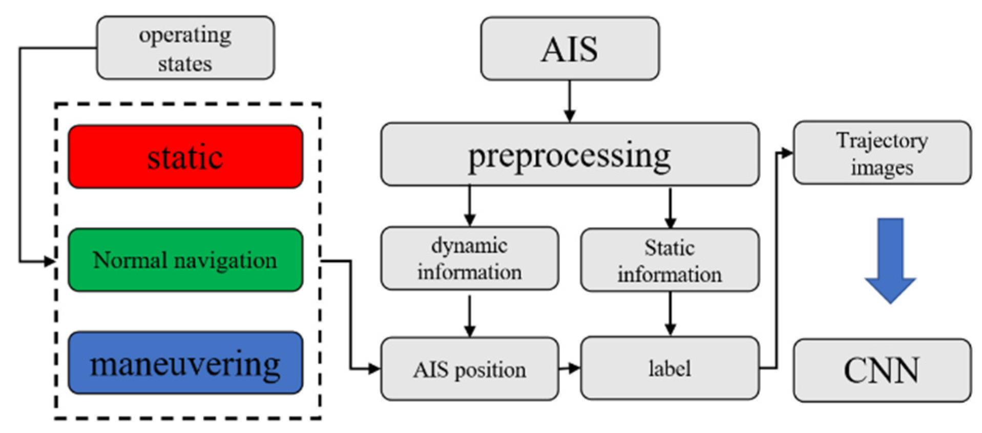
In this paper, the original AIS data is processed through data preprocessing, image generation and image labeling, and then the ship trajectory images with accurate labels are input into the convolutional neural network, so that the neural network is trained. Finally, the CNN model trained by a large amount of data is obtained, which can effectively classify the ship trajectory.

Figure 1 shows the schematic flowchart to illustrate the AIS data processing process.

2.1. AIS Data Format and Preprocessing

Considering the subsequent application processing process, the input AIS data types include Maritime Mobile Service Identify (MMSI), Vessel name, Vessel Type, Course over ground, Speed over ground, Latitude and Longitude. There are several considerations in choosing such a data structure.

• Considering the reality of the situation that the aforementioned static AIS information contains a certain degree of error information, it is not rigorous to determine the ship type of a specific ship only through the ship type data obtained in the AIS data, and such rash action may seriously affect the scientific nature of the entire study. Therefore, we chose to retain the MMSI number, ship name and ship type of AIS data at the same time and verify each other, to ensure the accuracy of the single ship type that will be used as the label.
• The two groups of dynamic data of course over ground (COG) and speed over ground (SOG) are also included in the algorithm input for two considerations. First, abnormal AIS data points can be identified by COG and SOG during data cleaning. Secondly, it plays a further role in the trajectory image generation stage.

After determining the data format of the input algorithm, a preliminary preprocessing of AIS data can be carried out. The first is to find out the AIS data which lacks the MMSI number, ship name and ship type. Since such data cannot effectively verify the accuracy of the ship type, it should be omitted. Secondly, if one of the three kinds of data is missing, for example, if the MMSI and ship type data are normal but the ship name data is missing, the ship type can be verified by the ship database. If the ship type associated with MMSI is consistent with the ship type transmitted in the AIS data, the data will be retained.

In addition, the data with obvious error in MMSI, such as the MMSI number shown as 0,1 or 9999, or latitude exceeding 90 degrees, longitude exceeding 180 degrees, are also cleared. Finally, the preprocessed AIS data is stored in CSV format.

2.2. Trajectory Image Generation and Tagging

After obtaining the pre-processed AIS data, the next step is to generate the trajectory image of each ship and label the image according to the type of the ship.

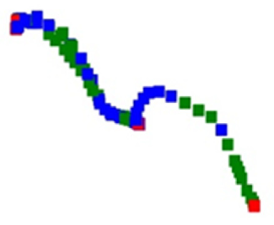
The specific processing of this part refers to the work of generating ship trajectory images in Xiang Chen’s research [16], and retains its division of ships under different operating states. Include (static, normal navigation, and maneuvering), and finally show themselves in the track images with three colors (red, green, and blue) respectively. This division is in the hope that through the differences in pixels, the differences in traffic characteristics, including handling characteristics, of different types of ships contained in trajectory images are highlighted to facilitate the following learning process of the neural network.

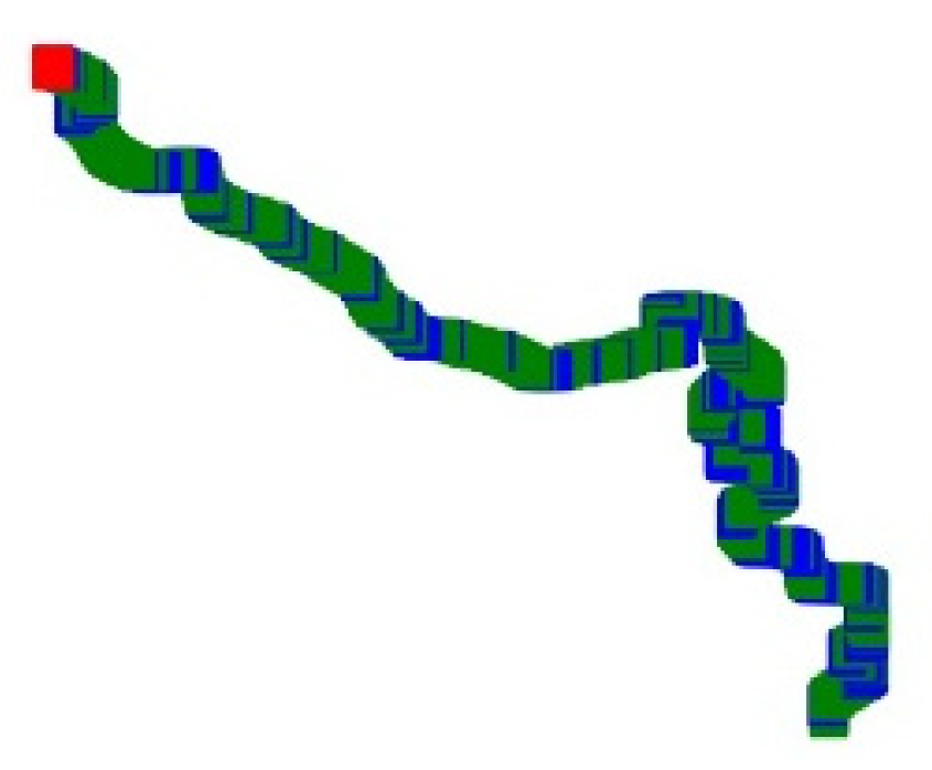
Figure 2 and Figure 3 shows the trajectory images of a passenger ship and an oil tanker, respectively. According to the division, the track segments under different manipulations will show different colors. In the part of the trajectory of normal navigation represented in green, there are sometimes blue parts, which means that the ship motion has a maneuvering process, especially when the direction of the ship’s motion changes. This is very visible in the second half of the track in 0.

Through the contrast of pixel colors in different areas in the picture, the type of movement states of the ship in the whole trajectory can be clearly identified.

The following part of the labelling processing is to store the trajectory images in different folders according to different types of ships to facilitate the construction and division of convolutional neural network data sets.

3. Image Classification Framework of CNN

Convolution neural network is a kind of widely used artificial neural network. The advantages of the convolutional neural network can be directly related to the convolution of the input image pixels, that is, directly extracted from the image pixel level image characteristics. This process is closer to the way the human brain and visual system process information than other methods.

3.1. The Input of Network

Trajectory images with three channels were selected as the input of the convolutional neural network. Each trajectory image represents AIS data in unit of one ship, where red, blue, and green represent trajectory segments of ships under different maneuvering conditions. After comprehensive consideration, the image size was set as (244,244) which is the usual pixel input size of most deep learning models. This size is used in some classic networks like VGG [20], ResNet [21] which means that each image has 59,536 pixels in it.

3.2. Convolution Layer

The biggest difference between convolutional neural network and other neural networks is that the convolutional layer is added in the network, that is, a kind of convolution calculation that can be directly carried out on two-dimensional data is added.

$$y(t)={\displaystyle \underset{-\infty }{\overset{\infty }{\int }}x(p)h(t-p)dp=x(t)\ast h(t)}$$

(1)

$$y(n)={\displaystyle \sum _{i=-\infty }^{\infty }x(i)h(n-j)=x(n)\ast h(n)}$$

(2)

The Equations (1) and (2) are continuous convolution operation formula and discrete convolution operation formula respectively. In the continuous convolution operation formula, x(t) and h(t) are convolution variable, p is the integral variable. In the discrete convolution operation formula, x(n) and h(n) represent the convolution variable, t is the parameter that shifts h(−i), and different t corresponds to different convolution results. Symbol * placed at the right part of the equations means convolution.

The convolution operation in a convolutional neural network is a discrete convolution: there are certain difference between convolution computation in the neural network and mathematics. Convolutional computation in convolutional neural network is to extract the features of the corresponding part of the image by using the movement of a convolutional kernel on the input image. The convolution kernel is also equivalent to a filter.

The size of the convolution kernel determines the size of the coverage region of the convolution kernel in the image, that is, the size of a convolution operation region, and the parameter values in the convolution kernel determine the influence ability of each pixel point in the image region covered by the convolution kernel on the final convolution result in this region. The greater the weight, the stronger the influence ability. The resulting weight sharing is also an important feature of the convolutional neural network, where a convolution kernel shares the same weight and bias value.

That is to say, the convolution of a convolution check image uses shared and identical parameters. The weights of sharing mode, greatly reducing the convolutional neural network in training the number of parameters need to learn, but at the same time, in this case, a convolution kernel can only extract and learn one feature of the input image. If a variety of different features of the image need to be extracted, multiple convolution kernels need to be used, that is, the image is repeatedly processed by using the convolution layer.

In addition, the movement mode of the convolution kernel can also be set when it moves, which is the concept of step size. The size and step size of the convolution kernel are important parameters that affect the size of the image output after the convolution calculation. The formula of the relationship between them is shown in Equation (3).

$$outpu{t}_s=\frac{inpu{t}_s-kerna{l}_s+2\times paddin{g}_s}{stride}+1$$

(3)

where input_s means the size of the origin photos, kernal_s is the size of convolutional kernel and stride means the sliding step.

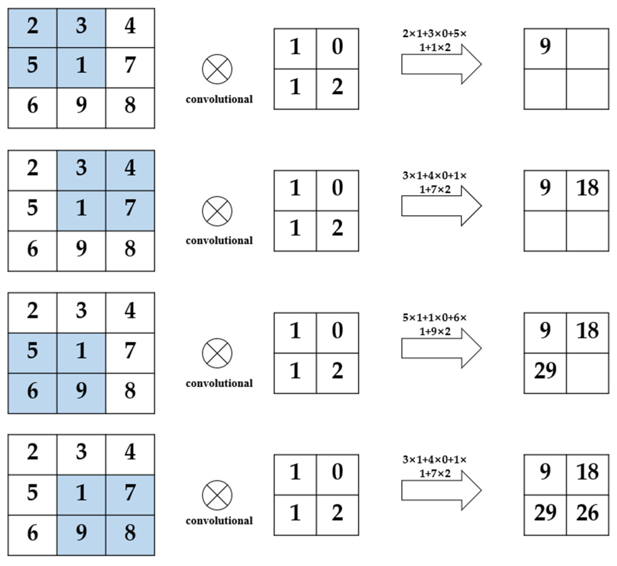
So far, the convolution process can be completed by setting the convolution kernel form and the convolution kernel move step. The example shown in Figure 4 is the complete calculation example of a 2 × 2 convolution kernel with stride 1.

3.3. Pooling Layer

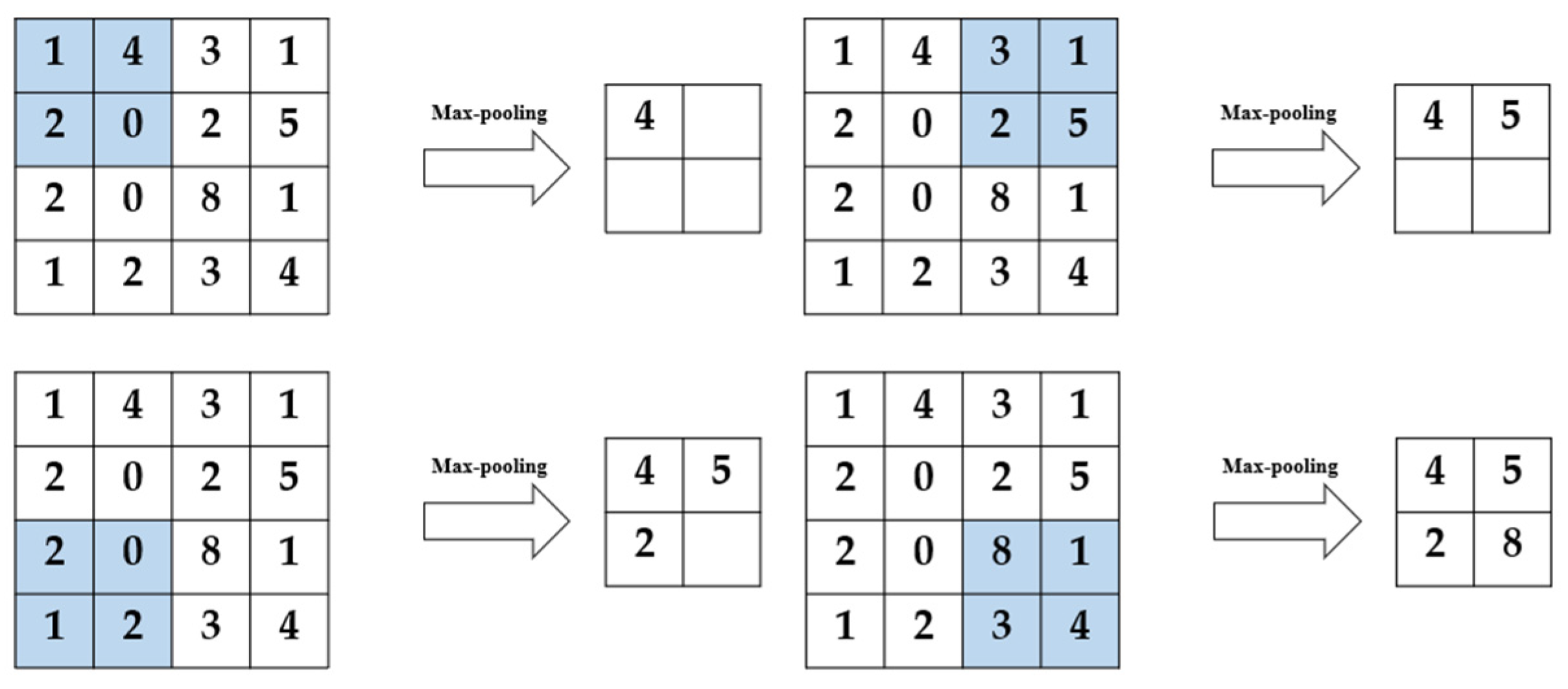
After the convolutional neural network extracts the features of the input image through the convolutional layer, a pooling layer is usually connected immediately after the convolutional layer, in such a way to further reduce the amount of data that needs to be calculated.

In this paper, the max-pooling method is adopted, and a 2 × 2 processing area is used to extract the point with the largest pixel value within the range of 2 × 2 in each step of pooling processing. The detailed processing is shown in the Figure 5.

3.4. Methods for Optimizing Performance

Optimization method often used in deep learning to improve performance mainly include increasing the training set size, regularization, and dropout. Considering the possible adverse effects of reducing network layers on classification performance, this paper mainly adopts batch norm and dropout methods to improve the performance of network and mitigate the potential overfitting phenomenon.

Batch norm in terms of its essence is not an optimization algorithm for deep neural networks, it is an adaptive parameter adjustment method that can overcome the model gradient problem caused by the increase of neural network layers to some extent. To explain it visually is to use a normalized function for an original value X to adjust the mathematical distributions such as the mean and variance of the original x.

In its application in neural networks, batch norm is used to normalize each hidden layer of neurons, the input distribution, which is gradually mapped to the nonlinear function, and then close to the limit saturation region of the value interval, is forcibly pulled back to the standard normal distribution with a mean of 0 and a variance of 1, and makes the nonlinear transformation function of the input values in the input-sensitive areas. This method can avoid the problem of gradient disappearance to some extent.

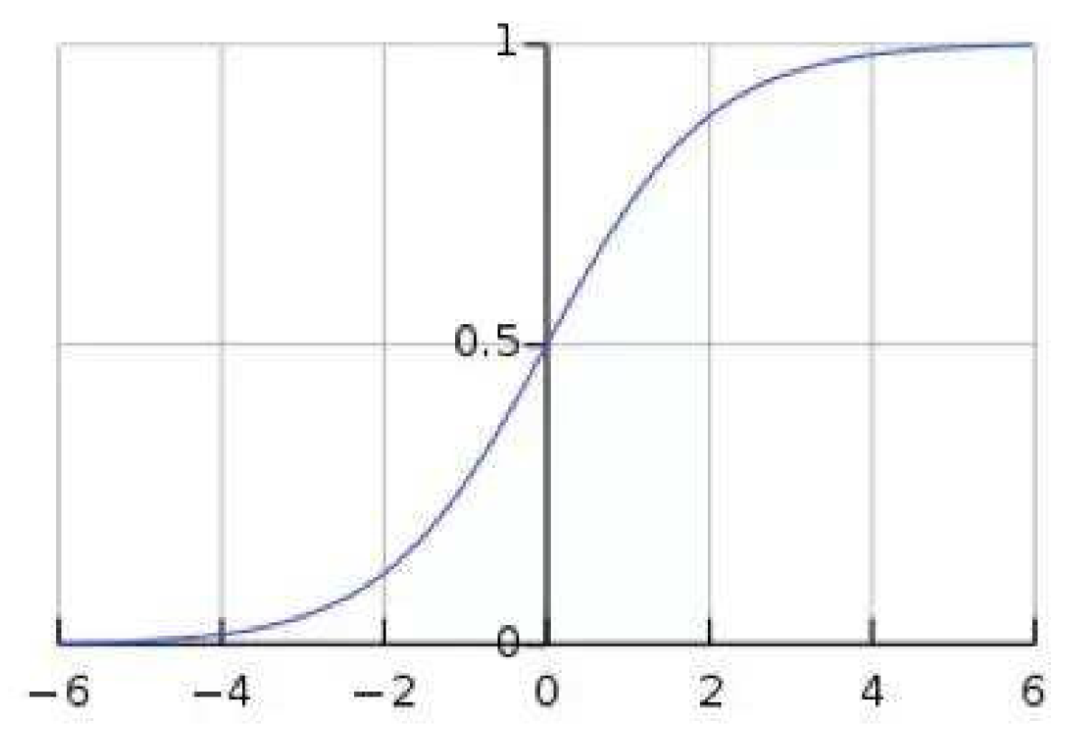
As shown as Figure 6, when using sigmoid to activate a function, as the depth of the network deepens, the distribution of the input value gradually shifts and approaches to the upper and lower ends of the value interval of the nonlinear function. In 0, toward the left and right ends of the Sigmoid function, that is, the parts that are closest to the X-axis, leads to the disappearance of the gradient during back propagation, which is also the reason for the slow convergence of the neural network.

After the batch normalization was adopted, the overall distribution of input values fell around (0, 0.5), as shown in the figure, which is the part with a large gradient, and could effectively avoid the problem of gradient disappearance. In addition, a large gradient also means a faster network convergence speed and training speed. By introducing some parameters in distribution adjustment, the phenomenon of overfitting can be alleviated to a certain extent.

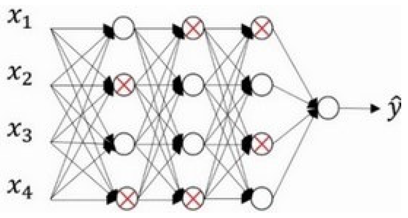
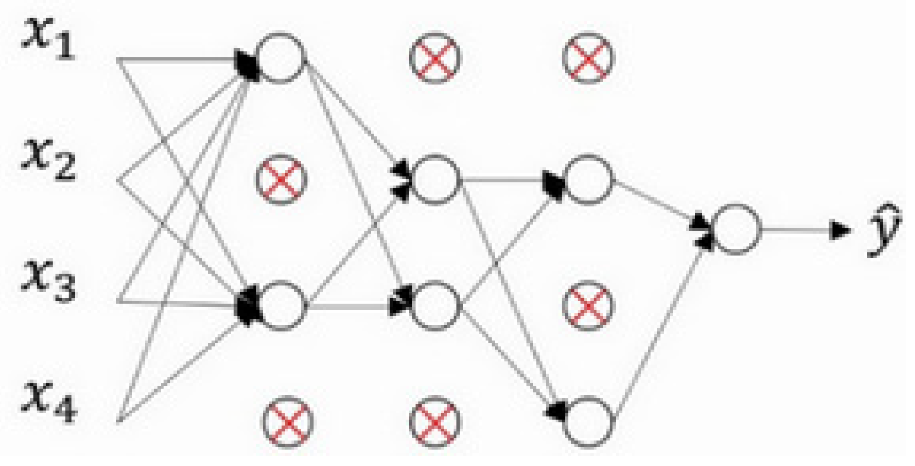
Dropout means random inactivation [22]. In network training, the output value of the neural node in the hidden layer is set to 0 with the set probability P. The dropout process goes from that shown in Figure 7 to that in Figure 8. Some neurons in Figure 8 are disconnected from the connections in the entire network. After this treatment, the neuron is disconnected, and then when the weight is updated by back propagation, the weight associated with the node is no longer updated.

Neural nodes in the hidden layer have a certain probability of being randomly inactivated, in other words, the training results of the network should not rely too much on a certain feature, because the input of the neural unit may be disconnected at any time, so that the update of the network weight also has a certain randomization. Dropout can effectively mitigate the occurrence of overfitting and achieve regularization to some extent [23].

3.5. The Selection of Activation Function

The activation function is an important part of the convolutional neural network, which determines the processing method of the output results of each layer in the neural network. If there is no activation function, then the output of each layer of the neural network simply accepts the linear combination of the results of the previous layer. No matter how many layers the network has, its final output is only the linear combination of the initial input. By introducing the nonlinear activation function, the nonlinear factors are introduced to the neurons in the neural network, so that they can deal with the linear inseparable problems and improve the expression ability of the neural network to the model.

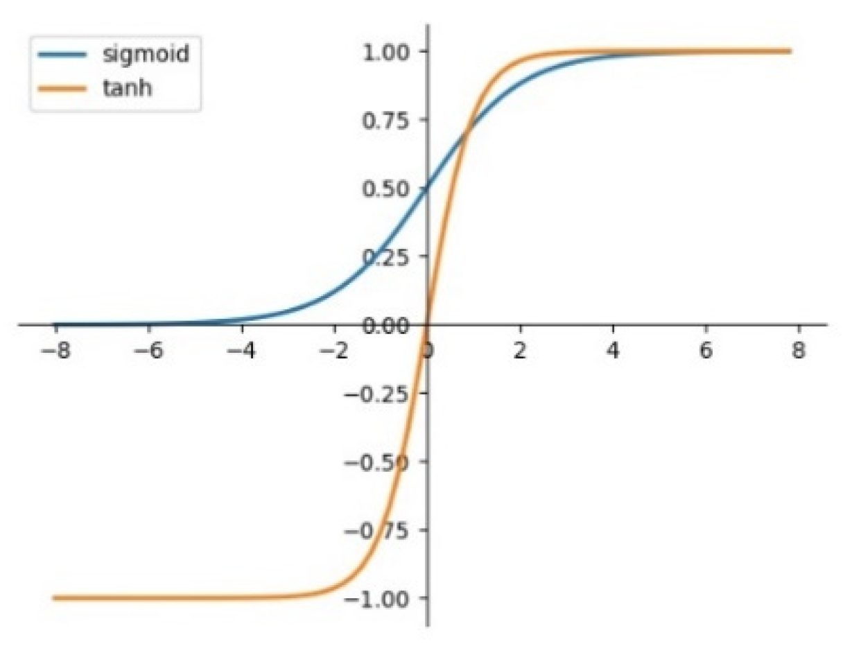
Several common activation functions in convolutional neural networks are sigmoid, tanh and ReLU. Their schematic is shown in Figure 9 and Figure 10.

The mathematical expression of these activation functions is shown in Equations (4)–(6).

$$sigmoid(z)=\frac{1}{1+e^{-Z}}$$

(4)

$$g(z)=\tanh (z)$$

(5)

$$\mathrm{Re}LU(z)=\max (0,z)$$

(6)

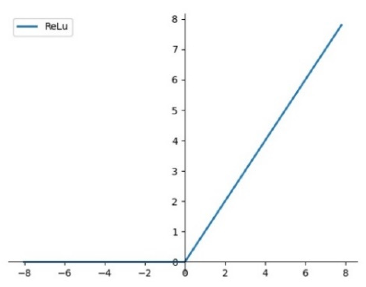
In this paper, the ReLU function is chosen as the activation function, as shown as in Figure 10 and Equation (6). If the input z is less than 0, the output of ReLU is always 0; When the input value z is bigger than 0, the output value of the ReLU function is equal to the input value z, and the derivative of the ReLU function is always 1.

Compared with other common activation function, back propagation with ReLU can better pass the residual to the front network layer, so that the parameters of the whole network can be updated more effectively. Meanwhile, the training time of convolutional neural network with ReLU is significantly shortened [24].

4. Data Analysis

Data is an important problem for any machine learning algorithm involved in classification: whether the selected data is extensive or not directly affects the final generalization performance of the network. This is especially true for ship trajectory data, as the trajectory performance of a ship in different water conditions and traffic conditions is not completely the same. Even for identical ships, in open water, narrow waterways, or port waters, their final trajectory characteristics are also different.

In addition, considering the differences in ship handling performance of different types of ships, the above-mentioned differences that exist in different external conditions may be further amplified. In order to adapt the model to a wider range of conditions, it is important to select ship trajectory data under different conditions as much as possible. In order to verify and optimize the proposed model structure, it is necessary to carry out actual data experiments.

For the above considerations, our experiments were performed on realistic ship trajectory data with different geometrical features and ship classes. Before the start of network training, data screening, processing, and feature analysis are essential parts.

4.1. Source of Original Data

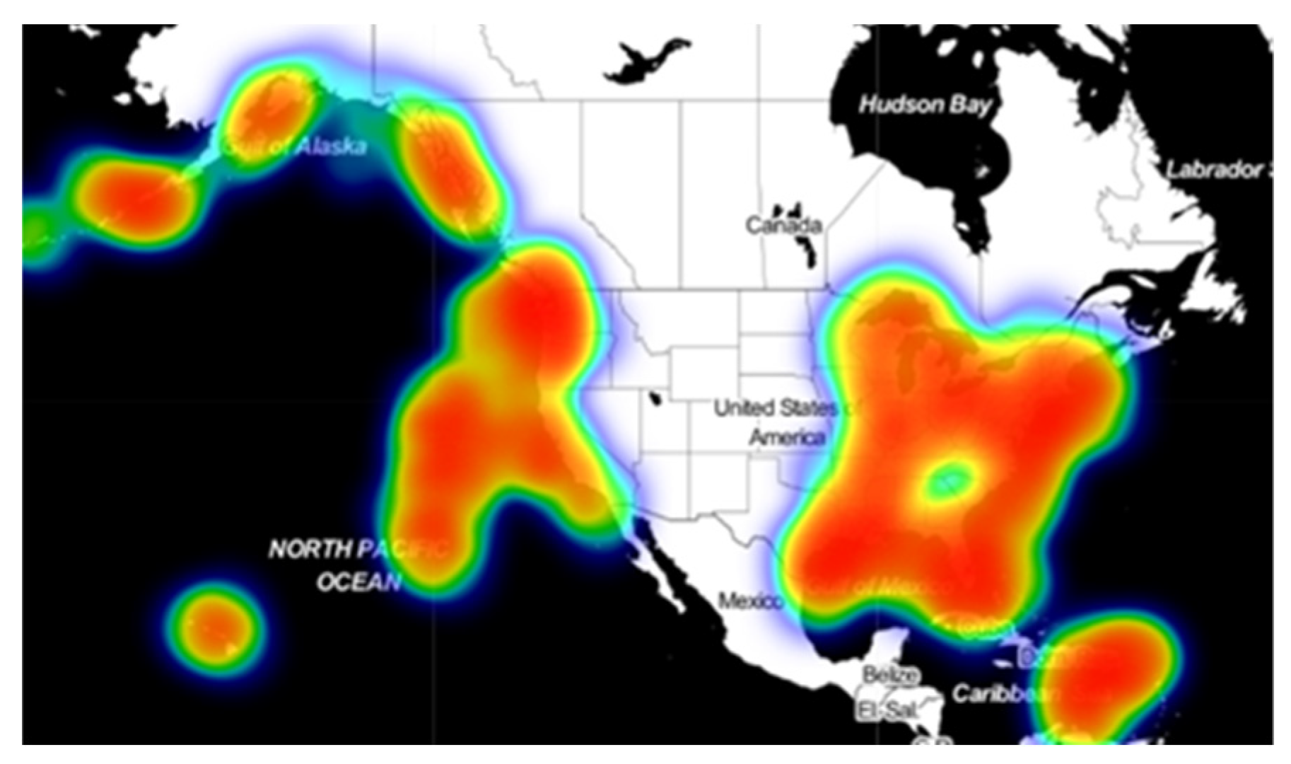
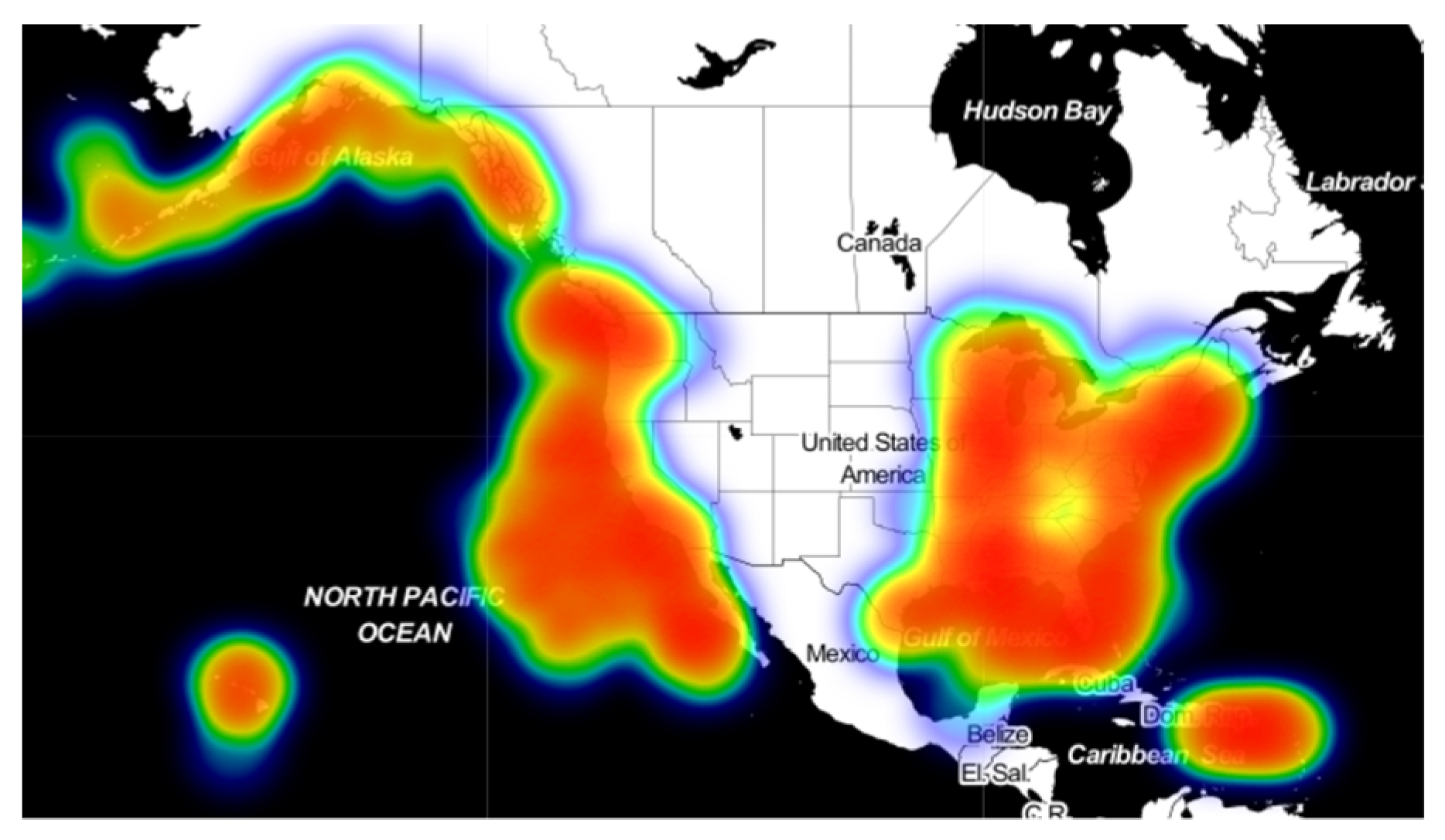
The data used in this article were from the U.S. National Oceanic and Atmospheric Administration’s Office of Coastal Management, with a time distribution of 25 days from 1 January 2019 to 25 January 2019. From the perspective of geographic space, it contains data of various types of waters with the United States as the main body. The data range includes inland waterways, lakes, ports, and open ocean areas around the United States. In such a large space, the diversity and universality of data can be effectively guaranteed.

Through visualization processing of AIS data of ships used in the research, the results are shown in the figures below. The data used in this paper are ship data which are distributed in North America. In the thermal map, the redder the color is, the more ships are sailing in this region, and there is a larger ship traffic density; conversely, the closer the color is to blue-green, the fewer ships are sailing in this part. According to the distribution in Figure 11, The data included in this study are widely distributed and show strong distribution characteristics. The Great Lakes region and the Mississippi River basin are the key areas of inland river and lake navigation in the United States. In addition, the east and west coasts, the Gulf of Mexico, and areas near the Hawaiian Islands also have high density distribution.

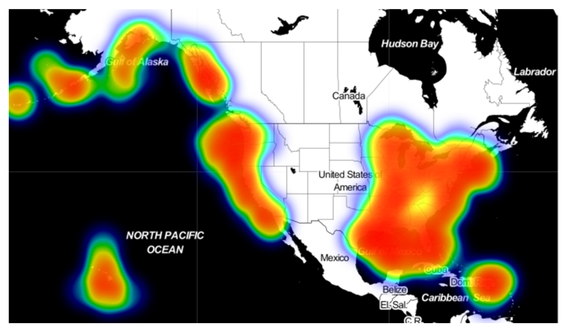
In order to further analyze the regulation of data distribution over time, AIS data of 15 January 2019 and 25 January 2019 were respectively generated as Figure 12 and Figure 13, namely the middle moment and the end moment of the overall data distribution selected by the research.

By comparison, it can be found that the distribution of ship traffic has also changed during the period of one month in January 2019, which is mainly reflected in the central region of the west coast. The situation is similar on the 1st and 25th, and there is an obvious decrease in the regional ship density on the 15th. Meanwhile, vessel traffic near the Hawaiian Islands showed the opposite trend, with the density distribution of ships near the 15th being significantly greater than that of the 1st and 25th.

In general, the overall data distribution is relatively uniform and extensive, achieving the desired purpose of incorporating diverse water conditions into the study. In addition, due to different water traffic conditions such as traffic flow direction, the diversity at the ship trajectory level is considerable.

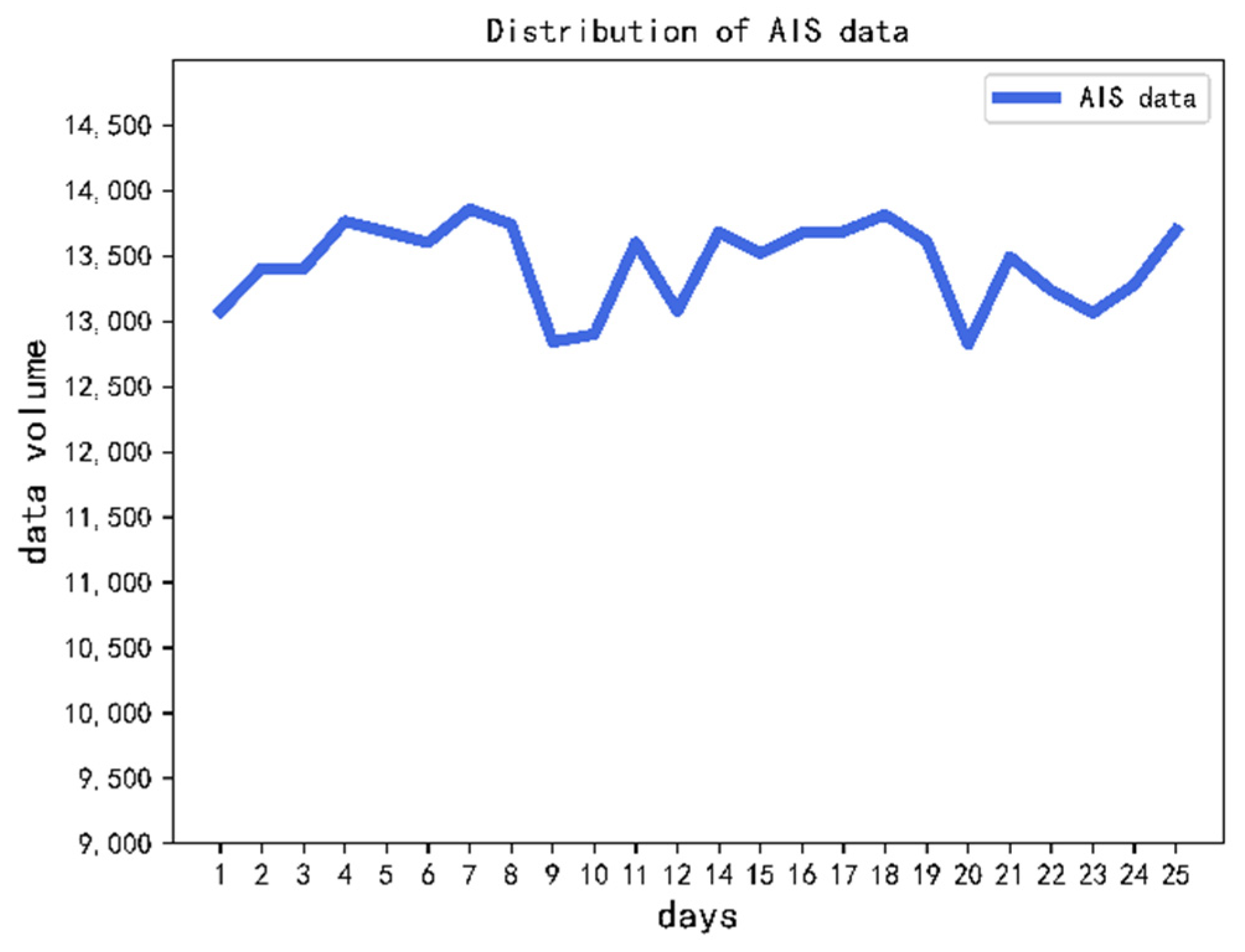
In order to facilitate subsequent track generation and processing and preliminary analysis of the ship’s AIS data, the original AIS data was first processed and stored as csv file in the unit of single ship.

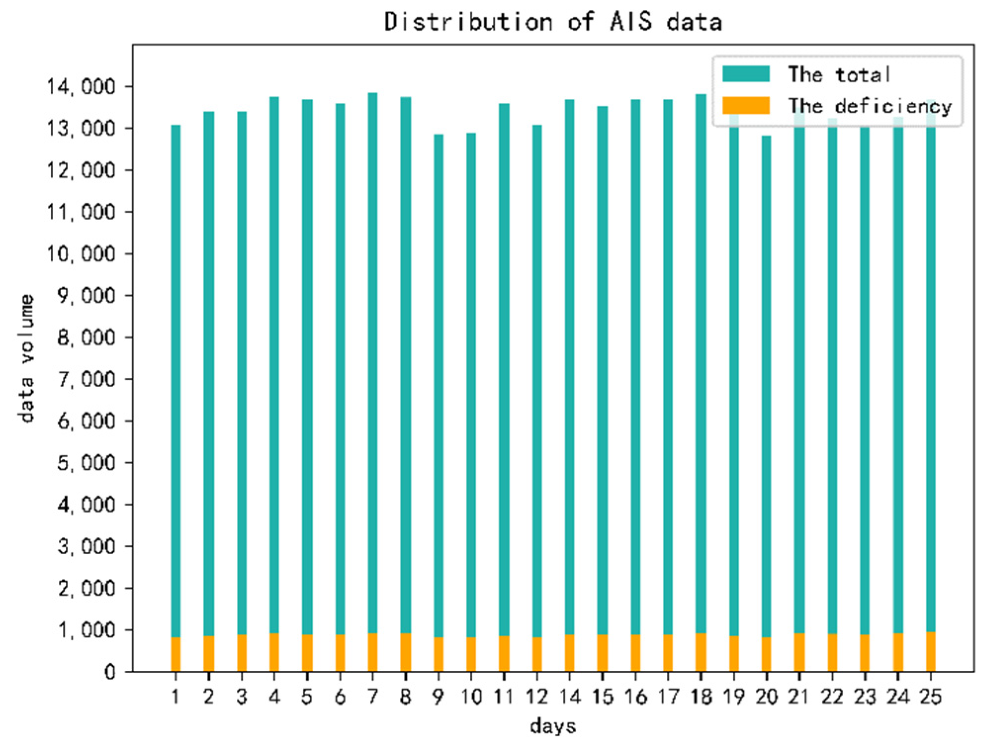
The distribution of processed AIS data with different dates are shown in Figure 14. Due to the amount of data that show obvious anomalies in 13 January, they were not used in the subsequent data processing. In general, the overall AIS data volume shows a stable trend. The daily record volume is stable at about 13,000 to 14,000 ships, AIS data of 327,021 ships were collected.

Before further processing of the initial AIS data, the quality and integrity of the data were analyzed. In order to make the data more intuitive, the statistics were still carried out in the unit of days. The main consideration was the absence of ship-name and ship-type data. If either or both of the two data sets are missing, the AIS data set of the current ship were marked as “missing” and statistics were made. The statistical results are shown in the Figure 15.

Similar to the overall date distribution of ships, the distribution of missing ship names or ship types in AIS data is also relatively stable. On average, 800 to 900 missing data are generated every day, accounting for 6% to 7% of the total data on that day. This result is also consistent with the situation that 6% of ship-type marking data are missing, as indicated by Abbas [12].

Missing data contribute to a certain extent to the stability of the distribution, but also from a side show that the present AIS data in the system on ship type data loss phenomenon is not accidental: there is an inherent problem in the completion of ship-type recognition research in addition to research significance, which also has certain actual application value.

4.2. Characteristics of Ship Types

After the initial AIS information is sorted and stored in the unit of a single ship, the distribution of ships by day was obtained as shown in the above section. Excluding the missing part of ship type information, the distribution of different types of ships can be obtained by computer processing.

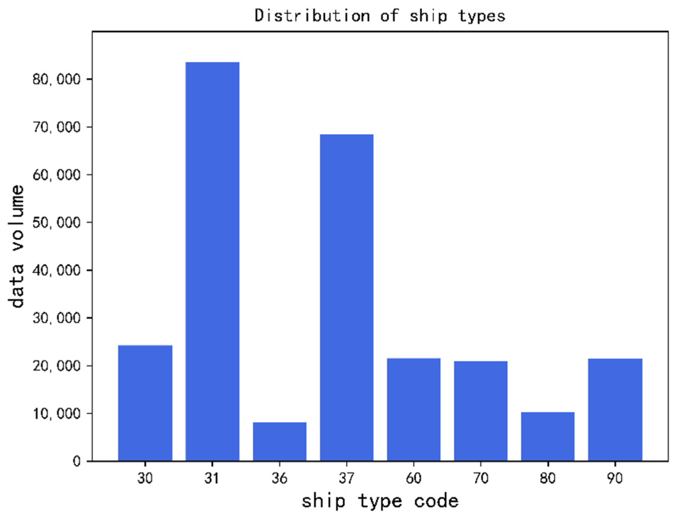
There are 258,812 AIS data of main ship types with complete and reliable final data accounting for about 79% of the initial AIS data volume. There are eight types of vessels: fishing boats, tow boats, sailing boats, recreational boats, passenger ships, pulp ships, crude oil products vessels, and work vessels. Ship types in the original AIS data are represented by corresponding codes. The corresponding relations between ship type code and ship type are shown in

Table 2. Ship type code and ship type.

Ship Type Code	Ship Type
30	Fishing boat
31	Tow vessel
36	Sailing vessel
37	Recreational vessel
60	Passenger vessel
70	Pulp vessel
80	Crude oil/product vessel
90	Other, working vessel

below.

As shown as Figure 16. Among them, tow boats and recreational boats are a large proportion, accounting for 32 percent and 26.4 percent, respectively. The AIS of sailboat type ships has the smallest data volume, accounting for only 0.3 percent of the overall data.

In addition to the eight main types of ships mentioned, there are other types of ships. However, considering the requirements of the convolutional neural network identification method adopted for the amount of data in the training set and the distribution of training data, in the subsequent network data input stage and the final classification stage of the full connection layer the input processing and classification of the above eight types of ships are mainly considered.

5. Experiment

For the training and optimization of convolutional neural network, the first work was to determine the specific structure of the neural network, including the number of network layers, the composition order of network layers, and the formal structure of the convolution kernel, etc.

After determining the network structure of CNN, it was also necessary to determine the values of some hyperparameters, including learning rate and epochs. This is usually a parameter tuning process that gradually tends to approximate the optimal. It was necessary to further adjust these hyperparameters according to the feedback of neural network training results after different parameter settings so as to achieve ideal image classification results for CNN.

In this paper, Keras, with TensorFlow as backup, was used to build the neural network. On the windows operating system, Python programming language was used to complete the computer implementation, and GPU was used to train CNN.

Finally, 16,000 data pieces were selected from 258,812 pre-processed AIS data pieces to generate ship trajectory images and form the data set of CNN.

To ensure the proportions of eight main types of ships were consistent, the specific approach of the generation of data set was achieved by random selection. We started with a random sampling of the same type of ship data, and the number of each type of ship trajectory images contained in the final data set was exactly 2000. This is a treatment that considers the principle of CNN training and learning. The average and random extraction of the corresponding data of all classified objects can, to a certain extent, eliminate the bias generated by human operation in the process of data set generation.

Eighty percent of the CNN data set were used as the training set, and 10% of the rest were used as the verification set and 10% as the test set. The specific partitioning of the data set is shown in the following

Table 3. Data set distribution table.

The Data Set	The Proportion	Dataset
Training set	80%	12,800
Verification set	10%	1600
Test set	10%	1600

.

5.1. Network Structure Construction

In the part of neural network construction and debugging in this paper, the strategy adopted was to first make a general determination of the network depth, that is, to determine how deep a network we generally need for feature learning for the currently prepared CNN data set. In this paper, three kinds of progressive network structures are proposed: model I, model II, and model III, as shown as

Table 4. Three basic structures of a network.

Layers	Model_I	Model_II	Model_III
Conv1	32	32	32
Conv2	32	32	32
Max-pooling	Yes	Yes	Yes
Conv3	64	64	64
Conv4	64	64	64
Max-pooling	Yes	Yes	Yes
Conv5	No	128	128
Conv6	No	128	128
Max-pooling	No	Yes	Yes
Conv7	No	No	256
Conv8	No	No	256
Max-pooling	No	No	Yes
Flatten	Yes	Yes	Yes
Dense	Yes	Yes	Yes

.

The main difference of the three different network composition structures lies in the number of convolutional layers in the convolutional neural network and the number of convolutional kernels on corresponding convolutional layers. The idea of such a setting also comes from the classical VGG Net [20] in the research field of convolutional neural network.

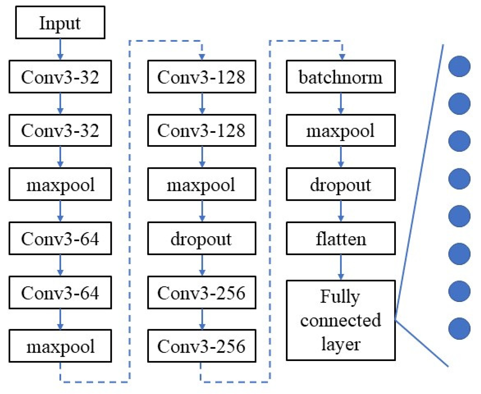
The three-layer network structure of two convolution layers plus one pooling layer is taken as a fixed module, where the convolution kernels are constructed in the form of (3,3). Such a setting of the convolution kernels conforms to the conclusion that small convolution kernels have certain advantages in VGG Net research [20]. The modules in this form are stacked to produce the three basic structures shown in 0. Structure I is the simplest and consists of six network layers: Conv1(32)-Conv2(32)-Max pooling-Conv3(64)-Conv4(64)-Max pooling.

Structure I has two such modules. Structure III can be obtained by stacking four such modules, in which the number of convolution kernels in different convolution layers is 32, 64, 128, and 256 respectively.

This structure inherits the simple and elegant features of VGG network. Due to the nature of the convolutional neural network, for networks composed of different depths, their sensitivity to some hyperparameters, including learning rate and batch size, is also different. For a set batch size, for example, set batch size = 16, its performance is different under different network structure settings. It cannot be assumed that the performance of a parameter on structure I will be similar to that of structure II or structure III because it performs better on structure I.

In order to form an effective, comprehensive, and intuitive comparison effect, the following hyperparameter debugging was also carried out in parallel based on the above three structures: independent testing and adjustment were carried out for structure I, structure II, and structure III.

5.2. Selection of Evaluation Index

The selection of machine learning evaluation indicators is also an important step in the whole process of neural network optimization training. For networks that involve target classification, a scientific and complete evaluation index system for different classification networks, including binary, multi-class, multi-labelled, and hierarchical has been developed [25]. These metrics are closely related to the confusion matrix [26].

The so-called confusion matrix is used to make statistics on the classification results generated by model classification, and count the number of targets incorrectly and correctly classified, respectively. It is the most basic and intuitive primary evaluation index to measure the classification performance of the model.

As shown in

Table 5. Confusion matrix.

Data Class	Classified as Pos	Classified as Neg
pos	True positive (TP)	False negative (FN)
neg	False positive (FP)	True negative (TN)

, it is a form of confusion matrix to evaluate the classification performance of the binary classification model: the correctness of a classification system can be evaluated by computing the number of correctly recognized class examples (true positives), the number of correctly recognized examples that do not belong to the class (true negatives), and examples that either were incorrectly assigned to the class (false positives) or that were not recognized as class examples (false negatives).

In summary, this paper studies the multi-type classification of ship types, so the corresponding confusion matrix is as shown in

Table 6. Confusion matrix of multi-class.

Ship Types	Classified as Type i	Classified as Other Types
Type i	True positive (TP)	False negative (FN)
Other type	False positive (FP)	True negative (TN)

.

According to the results of neural network classification of input images, the most easily thought of evaluation index is the correct proportion of all categories of images, namely average accuracy index, which represents the proportion of all correct results of the classification model in the total. The formula is shown in Equation (7).

$$Accuracy=\frac{TP+TN}{TP+TN+FP+FN}$$

(7)

In addition, there are indicators for the percentage of all outcomes predicted to be a certain category in the category. That is the precision indicator, Equation (8).

$$Precision=\frac{TP}{TP+FP}$$

(8)

Recall, also known as sensitivity index, refers to the case where the predicted value is consistent with the true value for classification problems, especially multi-type classification problems, Equation (9).

$$Sensitivity=\frac{TP}{TP+FN}$$

(9)

For classification problems, especially multi-type classification problems, in addition to the case that the predicted value is consistent with the true value (the proportion of completely correct classification, that is, the accuracy index), the case of incorrect classification generated by the model is also worth further analysis.

For example, objects with a certain type of true value are classified into other categories, which is the meaning of the recall indicator. Or the objects whose real values do not belong to a certain category are classified into the same category, which is the meaning of the precision index. These two types of errors generated in the classification of the model have certain reference significance, and enrich the index system for evaluating the performance of the convolutional neural network.

In addition to the above three indicators, namely accuracy, precision and recall, another evaluation index often used to evaluate the performance of classification models is F1score, which is a further indicator generated on the basis of precision and recall.

$$F1score=\frac{TP}{TP+\frac{FN+FP}{2}}$$

(10)

The F1score index combines the output results of precision and recall. The value of F1score ranges from 0 to 1, where 1 represents the best model output and 0 represents the worst model output.

6. Result Analysis

On the basis of the three basic structures of convolutional neural networks (structure I, structure II, and structure III), the classification performance of convolutional neural networks under four indexes (accuracy, precision, recall, and F_1score) under different network structures and different hyperparameters was analyzed.

6.1. Network Depth

For structure I, structure II, and structure III, shown in the 0, the network composition only includes the basic structure of the convolutional neural network, that is, the four layers structures including the convolution layer, the pooling layer, the flattening layer, and the fully connected layer, and they have certain progressiveness and similarity among each other.

When the batchsize parameter is set to 16, network learning training is conducted on structure I, structure II, and structure III until a certain epoch and network convergence, i.e., after the accuracy index becomes stable. The results are shown in the figure, and the three network structures with batchsize = 16 are named as I-A, II-A, and III-A, respectively.

According to the results shown in the

Table 7. Test accuracy of I-A, II-A and III-A.

Models	Accuracy
I-A	21.69%
II-A	32.6%
III-A	32.45%

, the accuracy of the model I-A with two ConV-ConV-Maxpooling combination reached 21.69% in the image classification, indicating that the convolution layer can extract certain features from the input image pixel data for the final classification of the fully connected layer. From model I-A to model II-A, the classification accuracy of ship trajectory images increased from 21.69% to 32.6%, which increased by nearly 10%. This shows that by deepening the depth of convolutional neural network and adding more convolutional layers to the network, the learning performance of features of the network can be improved and the classification accuracy can be improved.

On the other hand, the role of the convolutional layer in the convolutional neural network, especially the role of each convolutional kernel in the convolutional layer, is to learn and extract local features from the input images. By adding more convolution layers to the model I-A, the model II-A has a better performance in classification accuracy than the model I-A. That is to say, the network depth in the model I-A is insufficient, and only two layers in the model I-A cannot effectively extract some deep-level feature information.

Therefore, the deeper network depth of III-A is generated. Compared with II-A, two convolution layers with 256 convolution kernels are further added. However, the accuracy of III-A is almost the same as that of II-A, and the classification performance of the network does not show significant improvement. However, considering the influence of different batchsize and other hyperparameters, further analysis is needed for the model III-A. Only by comparing II-A with III-A, it cannot be determined that the six convolution layers contained in II-A can well extract the features in the image.

To sum up, two obvious conclusions can be drawn from the performance of the three models I-A, II-A, and III-A when the batchsize parameter is set to 16:

(1)

The I-A model containing four convolution layers cannot effectively extract features, and the network depth is insufficient.

(2)

III-A model needs to further adjust the parameters

6.2. Further Optimization

In this part, the proposed model is further optimized on the basis of the convolutional layer depth test in the convolutional neural network, to further improve its classification performance. Based on the conclusion (1), structure I was abandoned, and further adjustment and optimization were carried out on the basis of structure II and structure III.

The first is the selection of batchsize parameter. Considering that the input data set contains a total of 16,000 trajectory images, four different batchsize parameters, 8, 16, 32 and 64, were attempted.

Therefore, on the basis of the aforementioned II-A structure, with different batchsize parameter Settings, including the II-A structure at the beginning, i.e., the II-A-16 model when the batchsize was set to 16, there were four derivative models based on II-A structure. Their performance in accuracy index is shown in the

Table 8. The accuracy of model II under different batchsize.

Models	Batchsize	Accuracy
II-A-8	8	65.6%
II-A-16(II-A)	16	32.6%
II-A-32	32	76.5%
II-A-64	64	43.7%

.

Among the four models, the model II-A-32 had the best classification performance, that is, 76.5% classification accuracy, followed by the model II-A-8 with batchsize = 8 with 65.6% accuracy after training. In general, these four models show great changes and fluctuations in the accuracy index, and they are nonlinear. The two accuracy peaks are obtained when the batchsize value is 8 and 32, respectively. The remaining two batchsize values are 32.6% and 43.7%, respectively, which is approximately half of the better results. Such results also confirm the sensitivity of the convolutional neural network itself to the value of batchsize.

Similarly, on the basis of III-A structure, similar treatment was also carried out, and the results are shown in the

Table 9. The accuracy of model III under different batchsize.

Models	Batchsize	Accuracy
III-A-8	8	21.9%
III-A-16 (III-A)	16	32.45%
III-A-32	32	32.7%
III-A-64	64	43.6%

. For III-A structure, the accuracy index increased gradually with the increase of batchsize. By comparison with the above II-A structure, when the batchsize was 16 and 64, the two structures show A strong similarity in the accuracy index, and almost the same accuracy was obtained.

For the structure of III-A, the network was much deeper than that of II-A. Similar results were obtained under different values of batchsize, indicating that it is of little significance to further improve the classification performance of the network only by adding more convolution layers to the network composition. Next, we should consider adding other types of functional layers to the network in order to improve the classification accuracy again on the existing basis.

The first attempt was to add batch normalization to the network [27]. The essence of the neural network learning process is to learn about data distribution [28]. Therefore, the introduction of batch normalization to normalize the data in the network can improve the network promotion ability and speed up the training speed to a certain extent.

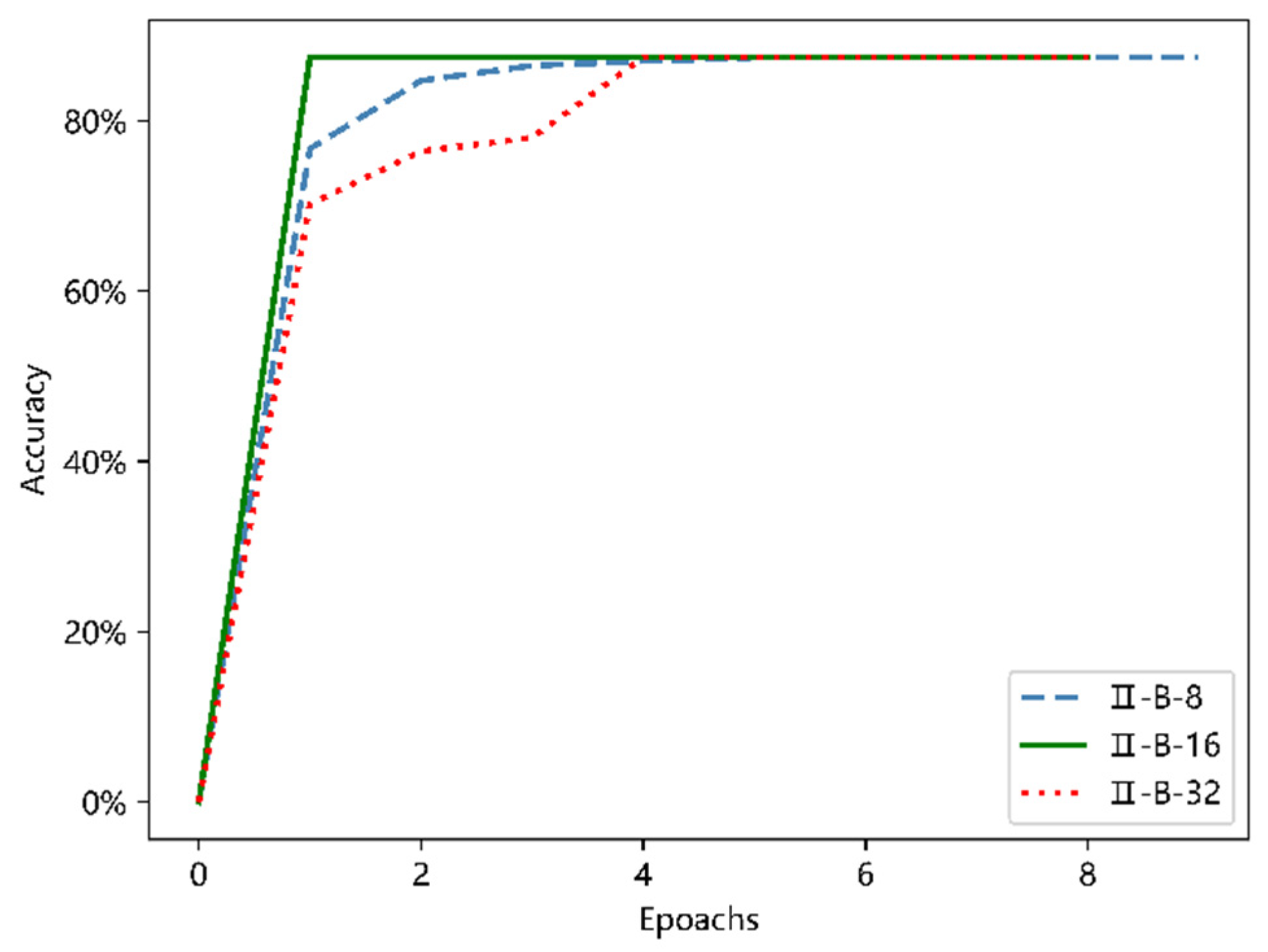
Similarly, the batch normalization layer was added to the II-A structure and III-A structure, respectively. In order to make the results more intuitive, they are shown in Figure 17 and Figure 18.

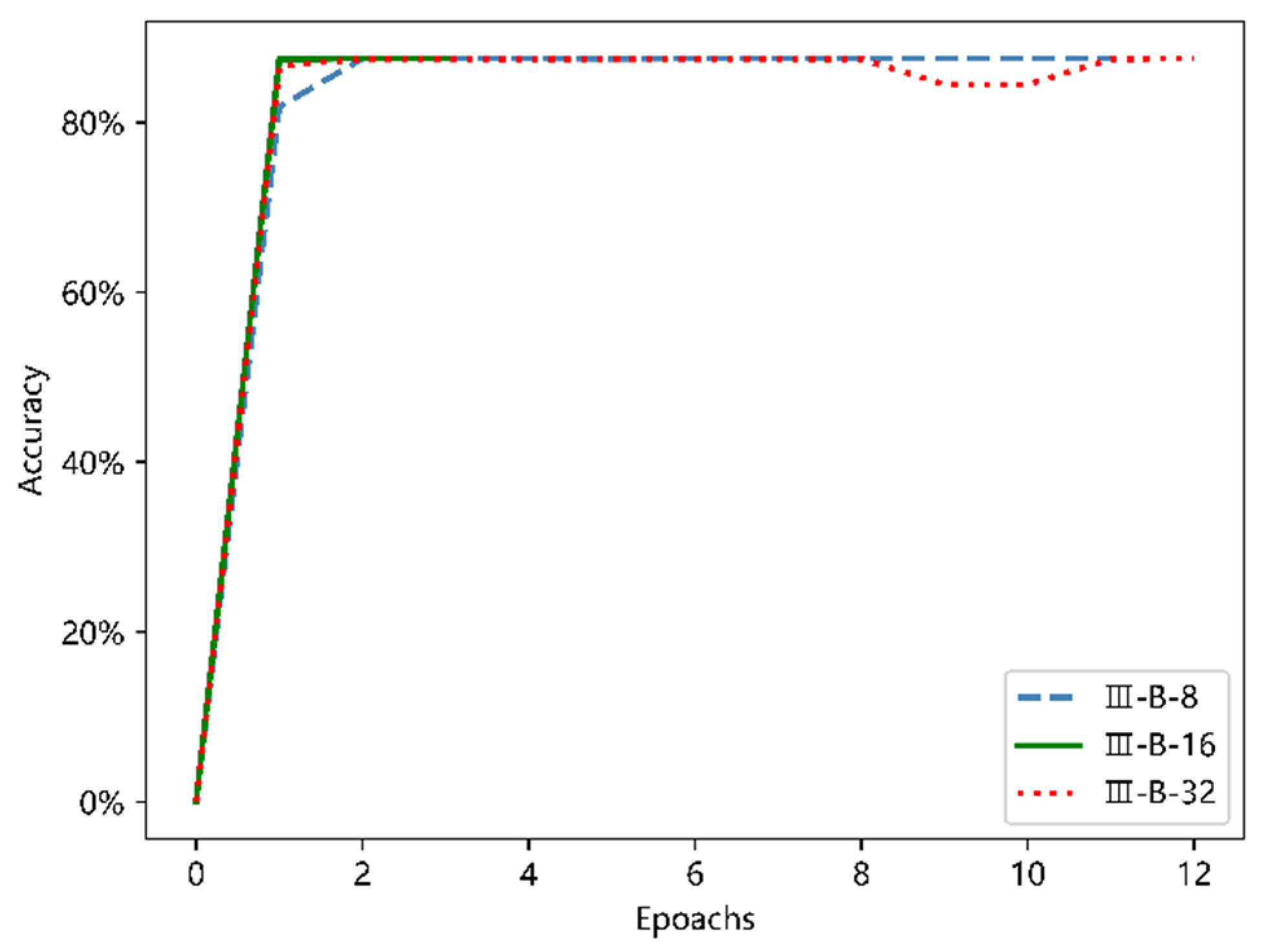
As shown in the two figures above, with the addition of the batch normalization layer to the network, the entire process from the beginning of training to near convergence was greatly accelerated, and compared with the maximum classification accuracy of 76.5% that the model would have achieved without the addition of the batch normalization layer, there was a 10 percent increase; when the network finally achieved convergence, the accuracy rate was stable to about 87.5%, which is consistent with the model II-B and III-B. From the comparison of the above two figures, the six models shown in the figure have very similar trends from the beginning of training to the basic convergence, and the common feature is fast convergence. However, in terms of stability and potential to deal with larger data sets later, the deeper network III-B model has the advantage.

The results shown in the Figure 17 and Figure 18 above also reflect the serious limitations of relying on a single accuracy index. The performance of the model III on other selected indexes is comprehensively analyzed in

Table 10. Accuracy, precision, recall, and F1 score on the model III.

Models	Accuracy	F1score	Precision	Recall
III-B-8	87.5%	0.2321	0.7351	0.1378
III-B-16	87.5%	0.0012	0.2	0.00062
III-B-32	87.5%	0.4491	0.3203	0.7511

.

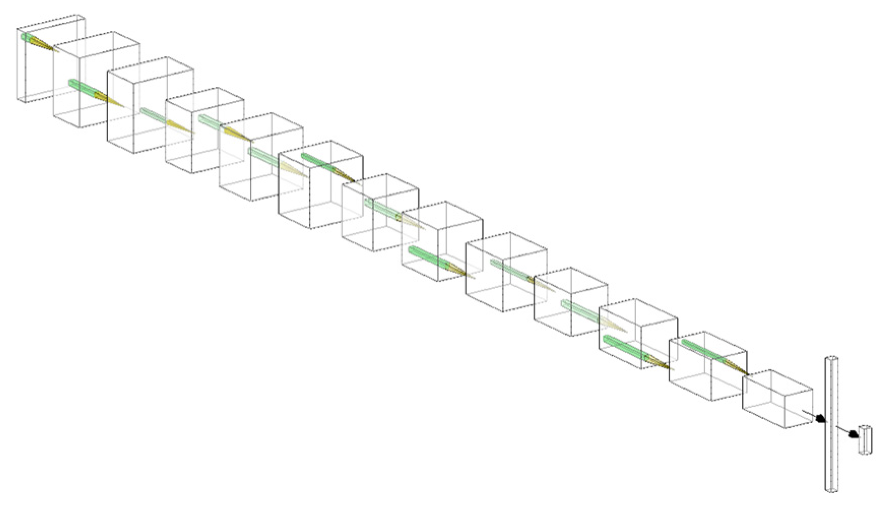
On the basis of the above indexes, it is proved that the proposed model III-B-32 has better performance in ship classification. The specific network structure of model III-B-32 is shown in the Figure 19 where each of these squares represents a specific layer in the convolutional neural network. It reflects the whole process from taking the ship trajectory picture as the input to finally completing the ship type identification and division. This is the final result of this paper. The stereoscopic diagram shown in Figure 20 corresponds to Figure 19, where the first square on the far left of the image represents the input of the whole convolutional neural network, i.e., the image input of 299 × 299 × 3. Then, through step-by-step convolution and pooling, it is finally connected to the fully connected layer on the right end, among which the square on the far right represents the classifier that will classify ship track images.

7. Conclusions

In this research, we propose a new CNN architecture for the purpose of ship classification. Firstly, ship motion features and trajectory shape features are extracted from a large number of AIS data of different types of ships, and trajectory images containing ship manipulation mode information are generated, which are used as input and basis for subsequent experiments. After that, a series of different experimental adjustments were made to CNN, from the depth and composition of network layer in convolutional neural network to the selection of super parameters, such as batchsize, in order to find out the optimal configuration of CNN. Finally, a network structure with good classification performance was proposed based on the comprehensive judgment of the selected multiple indexes.

In term of theoretical research, the ship type prediction model based on ship trajectory established in this paper was essentially an attempt to extract ship traffic characteristics. By introducing convolutional neural network, a traditional supervised learning method, into the study of ship classification, the ship type judgment and classification of unknown ship type trajectory can be achieved based on certain amount of sample data. Finally, the prediction results of ship type information classification can be used in many fields including information completion and verification.

In terms of practical application, this scheme can be directly applied to the maritime traffic research which take AIS data of the U.S. National Oceanic and Atmospheric Administration’s Office of Coastal Management as a data source. It will help researchers achieve a more reliable result in the process of ship type information completion or verification.

To the best of our limited knowledge, this paper presents a ship classification model based on ship trajectory image and convolutional neural network, by incorporating the division method of ships under different operating states into the process of ship trajectory generation, and we have achieved the establishment and verification of ship type recognition model in the context of self-created data sets. By adjusting the structure and parameters of the proposed model, we make the final classification result reach a considerable accuracy. The major limitation of the current work lies in the generation of trajectory images: although the ship trajectory pictures generated by the current method can reflect the ship’s state, they are still rough, and there are too many meaningless blank parts in the picture. Effective adjustment and optimization of the above problems will be the center of our future work. Future research will be carried out considering the following directions: (1) The generation process of ship trajectory image needs to be optimized and adjusted, and (2) we should consider choosing larger data volumes to achieve a better performance.