Ship Target Identification via Bayesian-Transformer Neural Network

Abstract

Ship target identification is of great significance in both military and civilian fields. Many methods have been proposed to identify the targets using tracks information. However, most of existing studies can only identify two or three types of targets, and the accuracy of identification needs to be further improved. Meanwhile, they do not provide a reliable probability of the identification result under a high-noise environment. To address these issues, a Bayesian-Transformer Neural Network (BTNN) is proposed to complete the ship target identification task using tracks information. The aim of the research is improving the ability of ship target identification to enhance the maritime situation awareness and strengthen the protection of maritime traffic safety. Firstly, a Bayesian-Transformer Encoder (BTE) module that contains four different Bayesian-Transformer Encoders is used to extract discriminate features of tracks. Then, a Bayesian fully connected layer and a SoftMax layer complete the classification. Benefiting from the superiority of the Bayesian neural network, BTNN can provide a reliable probability of the result, which captures both aleatoric uncertainty and epistemic uncertainty. The experiments show that the proposed method can successfully identify nine types of ship targets. Compared with traditional methods, the identification accuracy of BTNN increases by 3.8% from 90.16%. In addition, compared with non-Bayesian Transformer Neural Network, the BTNN can provide a more reliable probability of the identification result under a high-noise environment.

1. Introduction

Ship target identification is an important step in obtaining battlefield situation information. Moreover, in the civilian field, it can be used for maritime supervision, detection of suspicious vessels, and protection of maritime traffic safety. The ships may deceive supervision by tampering with identity information in Automatic Identification System (AIS) system, thus hiding the real identity and causing hidden dangers to maritime safety. In addition, with the development of autonomous ships, maritime traffic safety is a noteworthy problem. In the course of sailing, the autonomous ships need to identify and evade other targets effectively. Using tracks information to identify other targets can enrich the ways of identification and improve the target identification capability of autonomous ships.

Most studies identify targets by utilizing radar target polarization characteristics [1] and images [2,3]. However, when the radar target polarization characteristics are not obvious or target images are not clear, the above methods will be difficult to achieve. Therefore, an auxiliary target identification method using other information is needed. Time-series data are sequential data [4] which may make their features more discriminative [5]. The tracks of the ship targets are a kind of time series and have obvious time ordering. The tracks generated by different targets contain different motion information, which can help to identify the targets. Indeed, the ship targets’ identification using track information is a time series classification (TSC) task. The goal of TSC is to categorize time series into specific categories to facilitate better understanding and use of them. There are many methods that have been proposed to solve TSC. One paper [6] showed a distance-based approach, which used the Dynamic Time Warping (DTW) as the tool of similarity measurement. Time series are transformed into another feature space where the discriminatory features are more easily detected [7]. Another way to improve TSC performance is through assembling, whereby 35 classifiers are combined to achieve higher accuracy, named COTE [4]. However, target tracks are multidimensional time series and contain rich motion information, which is more complex and difficult to extract discriminant features. The traditional methods care less about the motion features and have no pertinence in solving the problem of tracks classification.

A growing number of researchers are focusing on target identification using tracks information. According to the characteristics of the track sequence, they have proposed some specific methods. Stephen Noyes [8] used a fuzzy logic method to identify the target as “wanted”, including aircraft, missiles, ships, and vehicles or “unwanted” including birds. Although he used a multi-valued logic, the memberships were too few to cope with a refined classification of targets. To address this shortcoming, Kouemou, G. and Opitz, F [9] made an improvement in the fuzzy logic approach. They considered more parameters of tracks, so more fuzzy membership functions were set up. Moreover, Doumerc et al. [10] added contextual information in the membership values of fuzzy logic. The target identification ability of fuzzy logic was enhanced. However, determining the fuzzy memberships and their functions required a lot of empirical knowledge and was challenging, especially when too many fuzzy memberships were considered. Wang Z.F et al. [11] built an air corridor model and then classified the tracks into airway targets and non-airway targets. However, it required a lot of prior information to establish airways, which was difficult to implement in a real-world environment.

With the development of the machine learning technology, many researchers tried to classify the tracks based on machine learning ways. Ghadaki, H. and Dizaji, R. [12] used a supervised learning technique named Support Vector Machines, which showed that machine learning methods performed well in target identification. More statistical features were extracted in [13]. L.P. Espindle et al. [14] used Gaussian mixture models to identify the target as aircraft or non-aircraft, and achieved a high accuracy of identification, but it needed the proportion of various target types. Kai Sheng et al. [15] proposed three movement patterns and extracted the features from these three patterns, which was novel and useful to extract more fine-grained features. Nevertheless, the features extraction process was complex. Yumu, D. et al. [16] designed an autoencoder to extract features and performed Principle Component Analysis (PCA) on them. Then, the Support Vector Machines, Convolutional Neural Networks and SoftMax were used to identify the targets. The method of feature extraction has been enriched. Considering that some targets were easy to distinguish while others may be harder, a multistage identification method was proposed in [17]. These methods enable machine learning to be well applied in track classification and made progress in track classification. Although the machine learning method is efficient and has been widely used, the construction and analysis of statistical features are complicated.

Rapid development of deep learning has indeed revolutionized the field of computer vision, especially with the advent of novel deeper architectures such as Residual and Convolutional Neural Networks [18]. Many researchers have also been applying deep learning methods to TSC. For instance, Hui Xing Tan et al. [19] used Long Short-Term Memory (LSTM) to detect various gait instances in different scenarios and environments. Kooshan, S. et al. [20] also used LSTM to achieve singer identification. Lai, C. et al. [21] developed a multi-stage deep learning-based model to automatically interpret multiple common ECG abnormality types. Meanwhile, the task of ship target identification by tracks information can also be processed by deep learning. Bakkegaard, S. [22] tried to use a RNN model to identify the ship target. Ichimura, S. and Zhao, Q. [23] proposed a MLP model to classify the cargo, fishing and passenger ships. The deep learning was proved to be feasible to solve the track classification. Nevertheless, the accuracy of the classification needs to be further improved. Moreover, a reliable predictive probability under high-noise environment is also needed, which is meaningful for the decision maker.

In this paper, the Bayesian-Transformer neural network (BTNN) is proposed to achieve more refined ship target identification (see Figure 1). Meanwhile, a reliable probability of the result under a high-noise environment can be provided, which is extremely significant in the fields of military and maritime surveillance. If the model misclassifies the sample and the predictive probability is still high, the predictive probability is proved to be unreasonable. On the contrary, if the model provides a low probability of the result, the commander will be alerted. The wrong decisions due to misclassification by the model will be avoided. The proposed model can capture both aleatoric and epistemic uncertainty. The weights of network are not fixed but follow a distribution. The encoder part from Transformer [24] is chosen with some simplification to build the Bayesian transformer encoders (BTE) module. The Bayesian transformer encoder (BTE) module is designed to get a discriminate representation of tracks in feature space, which can be seen as a feature extraction process. The features extracted by BTE module are flattened into one-dimensional feature vectors. Then, a Bayesian fully connected layer and a SoftMax function complete the classification and output the probability distribution. The Variational Inference (VI) [25] is chosen to train the BTNN. The model with the best performance during the training is selected. After training, BTNN can be used to identify ship targets using tracks information. BTNN performs well on a publicly available dataset Automatic Identification System (AIS). Compared with the traditional methods, BTNN achieves a higher accuracy. In addition, a more reliable probability of the result under a high-noise environment can be provided.

The main novelties are summarized as follows:

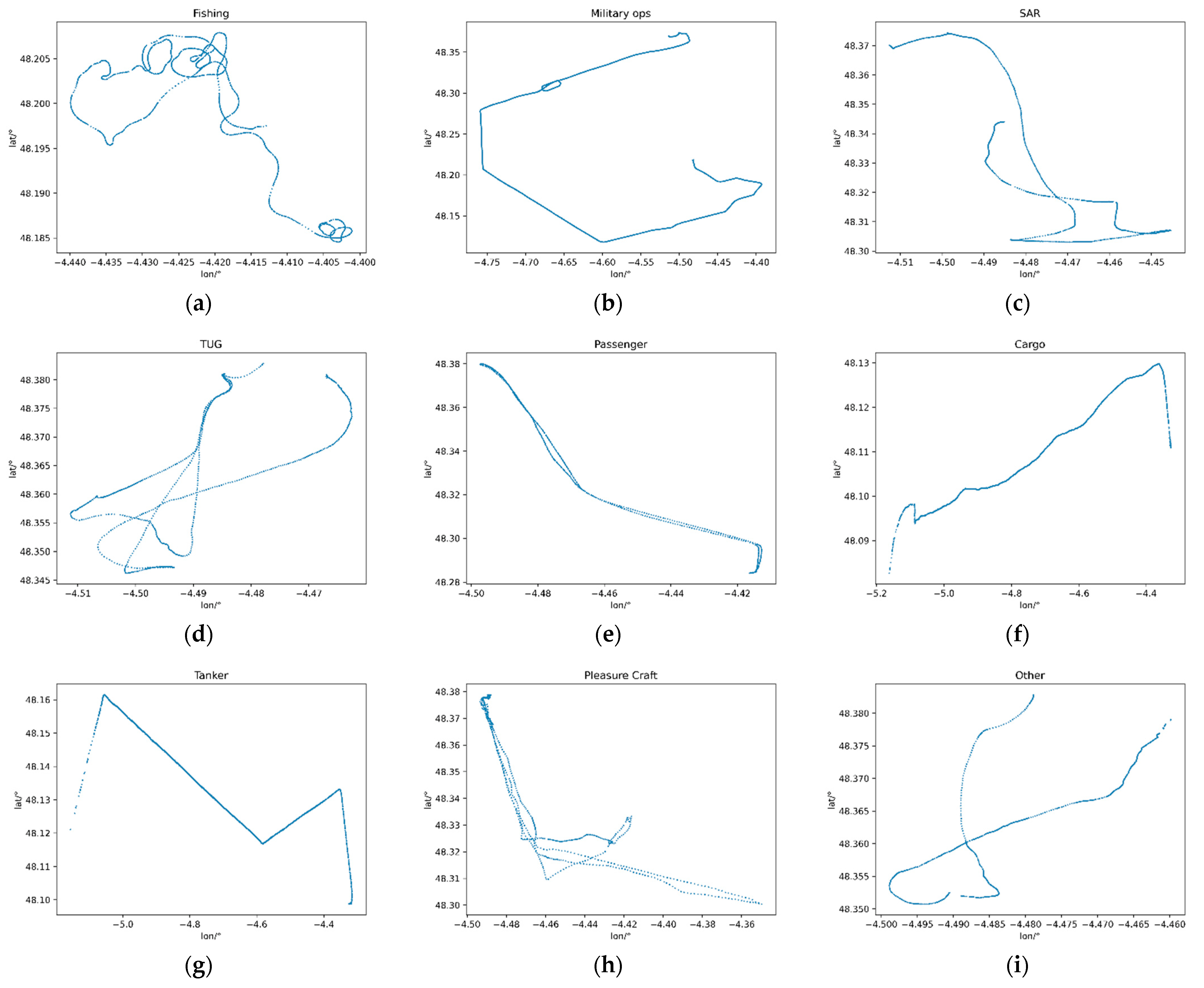
• The ship target is identified only by the track information.
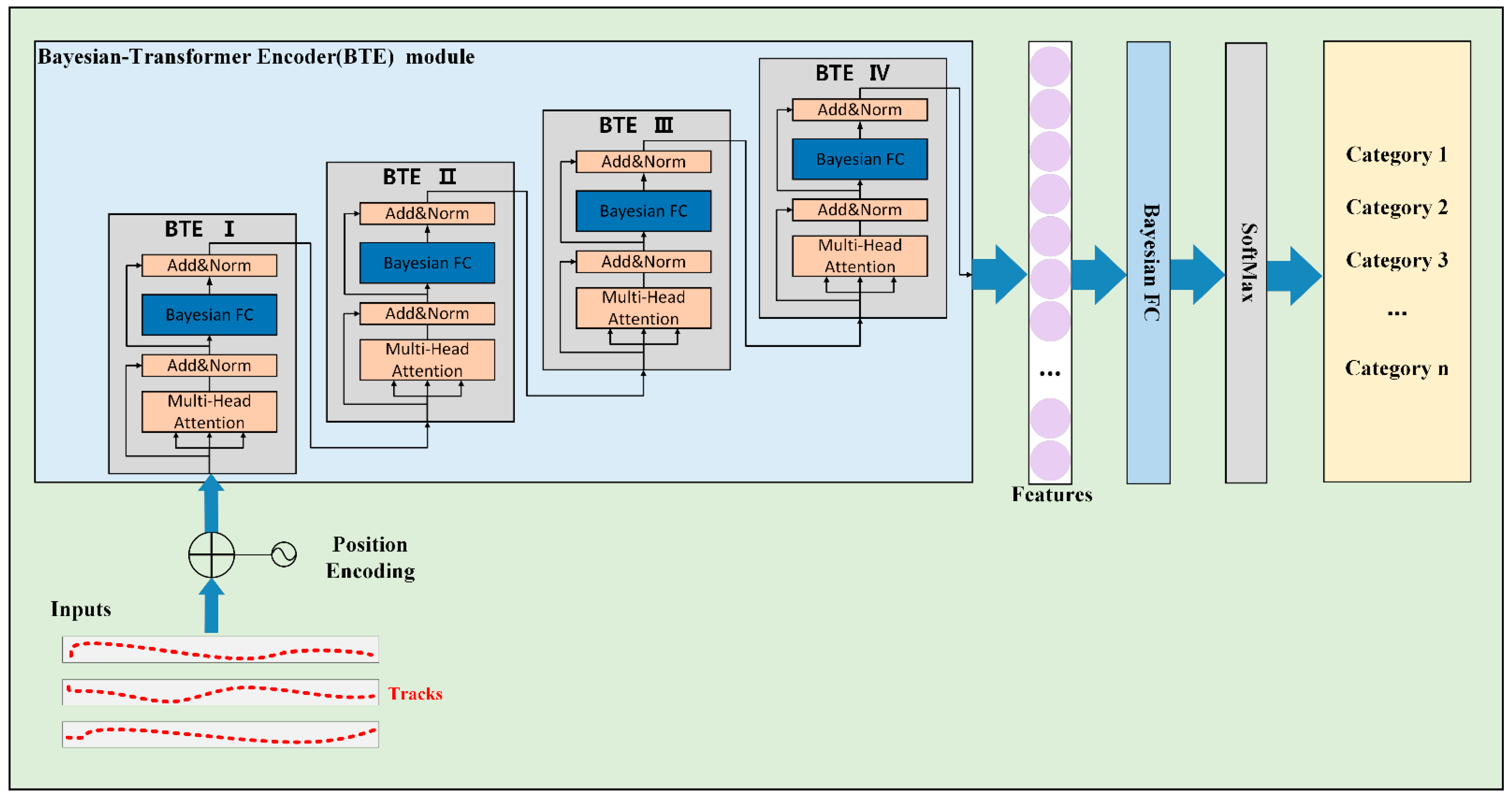
• To extract the discriminative features of tracks, a Bayesian-Transformer Encoder (BTE) module is proposed, which can deal with the long sequences and reduce network parameters.
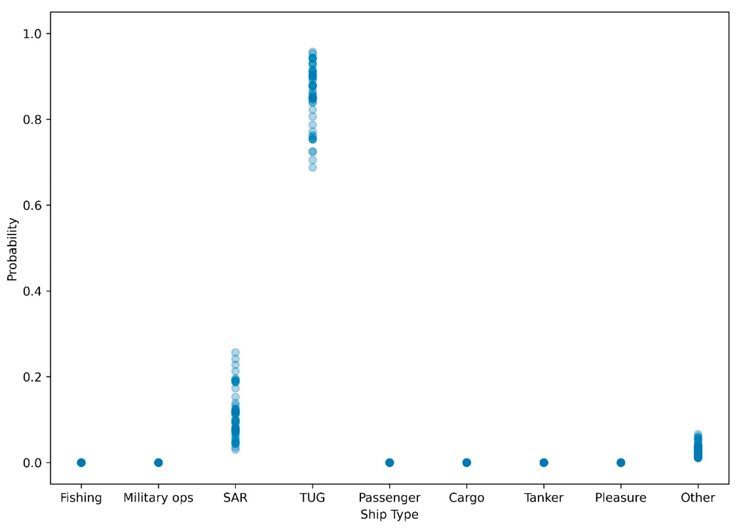
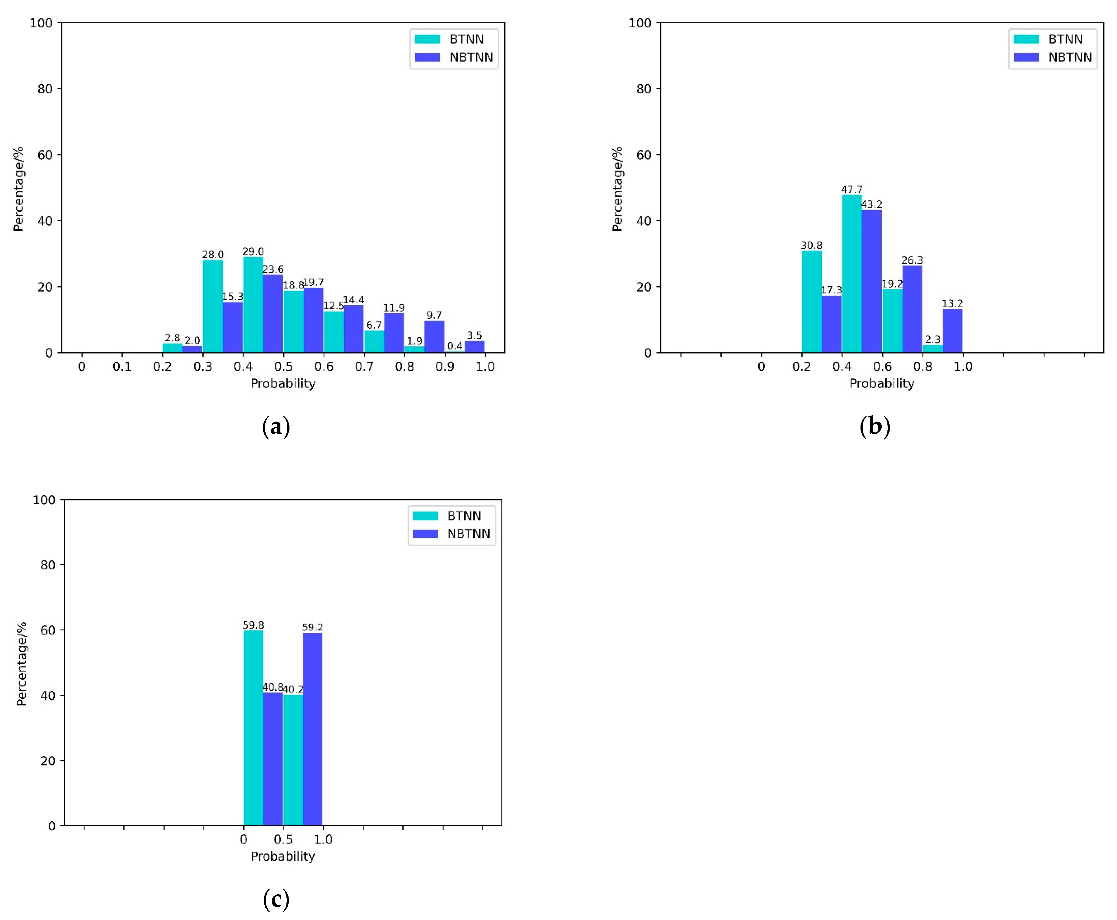
• The Bayesian principle is applied to the transformer neural network, which makes it possible to provide a more reliable probability that catches both aleatoric uncertainty and epistemic uncertainty.

This paper is organized as follows. Section 2 presents the proposed method. Section 3 displays the experimental results and analysis. Section 4 draws some conclusions.

2. Methods

2.1. Mathematical Model of Ship Targets Identification Using Tracks

Track samples could be represented as follows:

$${\mathit{T}}_i=\left\{{\mathit{P}}_{i1},\cdots ,{\mathit{P}}_{ij},\cdots ,{\mathit{P}}_{in}\right\}, j\in \left[1,n\right]$$

(1)

${\mathit{T}}_i$ represents the $i$th track in a track dataset $\mathit{T}$. $n$ is the total number of track points in ${\mathit{T}}_i$. ${\mathit{P}}_{ij}$ represents the $j$th track point in ${\mathit{T}}_i$.

$${\mathit{P}}_{ij}=\left(\begin{array}{l}\mathrm{latitude}, \mathrm{longitude}, \mathrm{speed} \mathrm{over} \mathrm{ground},\\ \mathrm{course} \mathrm{over} \mathrm{ground},\mathrm{time}\end{array}\right)$$

(2)

The task that ship target identification using tracks is to predict the ship target’s type based on $\left\{{\mathit{P}}_{i1},\cdots ,{\mathit{P}}_{ij},\cdots ,{\mathit{P}}_{in}\right\}$. The neural network is very sensitive to the singular value of data and the different distribution of data dimension during training. To avoid this adverse effect, 0–1 normalization is used to normalize track data. The formula of 0–1 normalization is shown in (3).

$$x_{ij}=\frac{x_{ij}-x_{\min }}{x_{\max }-x_{\min }}$$

(3)

where $x$ represents one dimension of the $j$th track point. $x_{\max }=\underset{i\in [1,m],j\in [1,n]}{\max }{x}_{ij}$, $x_{\min }=\underset{i\in [1,m],j\in [1,n]}{\min }{x}_{ij}$, $i$ is the number of the track.

2.2. Overall Structure of BTNN

The tracks generated by ships contain a wealth of features of the targets. The main idea of the proposed method is to predict the type of ship targets by tracks information. Tracks are multidimensional time series. Every track belongs to a certain target type $y_i$, which is selected to be the label of the track ${\mathit{T}}_i$. The training of BTNN based on tracks is a supervised learning process. BTNN consists of four parts: Position Encoding, Bayesian-Transformer Encoder module, Bayesian Fully Connection (FC) and SoftMax. (see Figure 1), First, the position of track points is encoded. Track is a discrete time series, so all points have a definite order. By this, the position of the track points in “Position Encoding” is encoded. The function of positional encoding is:

$$\begin{array}{l}PE\left(p,2i\right)=\sin \left(p/{10000}^{2i/d}\right)\\ PE\left(p,2i+1\right)=\cos \left(p/{10000}^{2i/d}\right)\end{array}$$

(4)

where the $p$ represents the position, the $i$ is the $i$th dimension of the position $p$. The $d$ is the dimension of one position. Second, the Bayesian-Transformer Encoder module is used to extract features and obtain another representation of the track. Third, the new representation is transferred in Bayesian FC layer. Finally, the SoftMax outputs probability distribution and completes the classification. The weight parameters in the BTNN follow a distribution $p\left(w|T,Y\right)$, which is to be obtained by variational inference [25]. The core part of the BTNN is illustrated in detail in Section 2.3. The application of Bayes principal in the BTNN is stated in Section 2.4.

2.3. Bayesian-Transformer Encoder (BTE) Module

The transformer network [24] was originally designed for machine translation problem, which is a sequence to sequence task. The transformer includes an encoder part and a decoder part, which has eschewed recurrence and instead relies entirely on an attention mechanism. Therefore, the transformer is capable of parallel computation. In view of these advantages, the transformer structure is used to achieve the classification of track. However, target identification is a classification task. The input is a multi-dimension sequence, and output is the target type that can be represented as a number. Unlike machine translation problem, there is no need to generate and output a new sequence. Therefore, a Bayesian FC layer and SoftMax are used as the decoder. There are mainly two parts in the transformer encoder layer: multi-head attention and feed forward. The attention mechanism is used to capture relationship between different data points in the input sequence. The attention function is defined as:

$$\mathrm{Attention}(Q,K,V)=\mathrm{softmax}\left(\frac{Q{K}^T}{\sqrt{d_k}}\right)V$$

(5)

where the queries $Q$, keys $K$ and values $V$ are the linear projection of the input. The attention mechanism can get the weights of every $K$ to the $Q$, then the values corresponding to the $Q$ are computed by Equation (4). The function of multi-head attention is:

$$\mathrm{MultiHead}(Q,K,V)=\mathrm{Concat}({\mathrm{head}}_1,\cdots ,{\mathrm{head}}_h)W^O$$

(6)

$${\mathrm{Head}}_i=\mathrm{Attention}(Q{W}_i^Q,K{W}_i^K,V{W}_i^V)$$

(7)

The $W_i^Q,W_i^K,W_i^V$ and $W^O$ are parameter matrices to realize the linear projection. The multi-head attention makes it possible to care about different information in different subspaces. The feed forward part consists two fully connection (FC) layers, where dimensions of data increase first and then decrease to be the same as the input sequence. However, there is no need to make the output and input dimensions of the Bayesian-Transformer encoder the same; instead, the dimension in Bayesian-Transformer encoder output is changed. In the second part of the BTNN, four Bayesian-Transformer encoders (BTE) are used (BTE I, II, III, IV). There is only a Bayesian FC layer in the feed forward part. The output and input of BTE I have the same dimensions, as does BTE III. However, the output and input of BTE II have different dimensions. BTE IV also has different output and input dimensions. The feed forward of BTE II only increases the dimension $d_1$ of data, thus providing a higher dimension input for BTE III. Increasing dimensions of data points in the input sequence can provide richer information for the calculation of attention, and the encoder layers can better extract the feature information among different points in the input sequence. Furthermore, the number of parameters in feed forward part is also reduced. The output of BTE IV is flattened out to get a discriminative feature vector, which is another representation of input. The dimension $d_2$ of the discriminative feature vector depends on the feed forward of BTE IV. The experiment in Section 3.2 shows that the BTNN is both reasonable and effective. Additionally, the best values of $d_1$ and $d_2$ are also selected.

2.4. Bayesian-Transformer Neural Network (BTNN) Training and the Predictive Probability Calculation

In Bayesian-Transformer Neural Network (BTNN), predictive uncertainty comes from two different sources: aleatoric uncertainty and epistemic uncertainty. Aleatoric uncertainty captures the inherent uncertainty in data and epistemic uncertainty expresses the model uncertainty [26]. BTNN can reflect both epistemic uncertainty and aleatoric uncertainty, while Non-Bayesian Transformer Neural Network (NBTNN) can only express aleatoric uncertainty. The reason is that NBTNN has fixed weight parameters, but the weights of BTNN follow a distribution $p\left(w|T,Y\right)$, which satisfies the following Bayes formula:

$$p\left(w|T,Y\right)=\frac{p(T,Y|w)p(w)}{p(T,Y)}$$

(8)

where $w$ is the set of model parameters, $T$ is the track dataset, $Y$ is the label of the track. $p\left(w|T,Y\right)$ is the posterior. It is the probability of the $w$ conditioned on the data $\left(T,Y\right)$. $p\left(w|T,Y\right)$ is difficult to compute by Equation (8). Jordan, M.I. et al. [25] provided a variational inference (VI) method to approximate the complicated posterior distribution $p\left(w|T,Y\right)$ by a simpler one called variational distribution $q_{\theta }\left(w\right)$. $\theta$ is the set of variational parameters describing the proposed distribution. The process of BTNN training is finding a $q_{\theta }\left(w\right)$ to approximate $p\left(w|T,Y\right)$. The Kullback–Leibler (KL) divergence is used to measure the similarity between $q_{\theta }\left(w\right)$ and $p\left(w|T,Y\right)$.

$$\mathrm{K}\mathrm{L}\left\{q_{\theta }\left(w\right)\left|\right|p\left(w|T,Y\right)\right\}={\displaystyle \int q_{\theta }\left(w\right)\log \frac{q_{\theta }\left(w\right)}{p\left(w|T,Y\right)}dw}$$

(9)

The goal is to minimize $\mathrm{K}\mathrm{L}\left\{q_{\theta }\left(w\right)\left|\right|p\left(w|T,Y\right)\right\}$. The right side of Equation (9), $p\left(w|T,Y\right)$ can be replaced by $p\left(w,\left(T,Y\right)\right)/p\left(T,Y\right)$, and the Evidence Lower Bound (ELBO) can be obtained:

$$\mathrm{E}\mathrm{L}\mathrm{B}\mathrm{O}\mathrm{=}{E}_{q_{\theta }(w)}\left[\log \left(p\left(T,Y|w\right)\right)\right]-\mathrm{K}\mathrm{L}\left[q_{\theta }\left(w\right)\left|\right|p\left(w\right)\right]$$

(10)

Maximizing the ELBO is the goal to optimize. The parameters in the VI model are replaced by Gaussian distributions:

$$w\sim q_{\theta }\left(w\right)=N\left({\mathsf{\mu }}_w,{\mathsf{\sigma }}_w^2\right)$$

(11)

According to [27], reparameterize the random variable $w$ as:

$$w={\mathsf{\mu }}_w+ϵ{\mathsf{\sigma }}_w,ϵ\sim N\left(0,1\right)$$

(12)

Thus, the backpropagation can be achieved through $w$ because $ϵ\sim N\left(0,1\right)$ has no tunable parameters and does not need to be updated.

After the model has been trained, it can be used to predict the category of the tracks. Here, the calculation of predictive probability is stated. The same inputs $T_i$ are predicted for $H$ times. Every time a multinomial conditional probability distribution (CPD) is obtained $p(Y_i|T_i,w_t)$ = Multinomial distribution with $n$ target classes (MN) $\left(p_{{}_1}^t\left(T_i,w_t\right),\cdots ,p_{{}_k}^t\left(T_i,w_t\right),\cdots ,p_c^t\left(T_i,w_t\right)\right)$, where $t\in [1,2,3,\cdots ,H]$. Every time the MN under BTNN is corresponded to a sampled weight constellation $w_t$ [28]. For each class $m\in \left[1,2,3,\cdots ,c\right]$, the mean probability can be determined by:

$$p_m(T_i,w)=\frac{1}{H}{\displaystyle \sum _{t=1}^H{p}_m^t}(T_i,w_t)$$

(13)

Then, the class of the target is predicted by the highest mean probability $\max (p_m(T_i,w))$. Now, the predictive probability is achieved:

$$p_{pred}=\max \left(\frac{1}{H}{\displaystyle \sum _{t=1}^H{p}_m^t}(T_i,w_t)\right)$$

(14)

As the Figure 2 intuitively shows, the aleatoric uncertainty is expressed in the distribution across the classes, which is zero if one class receives a probability of one. The epistemic uncertainty is expressed in the spread of the predicted probabilities of one class, which is zero if the spread is zero [28]. Therefore, the BTNN can provide a more reliable predictive probability calculated by Formula (10) that captures both aleatoric and epistemic uncertainty. The advantage will be further demonstrated through experiments in the Section 3.4.

3. Experiments and Analysis

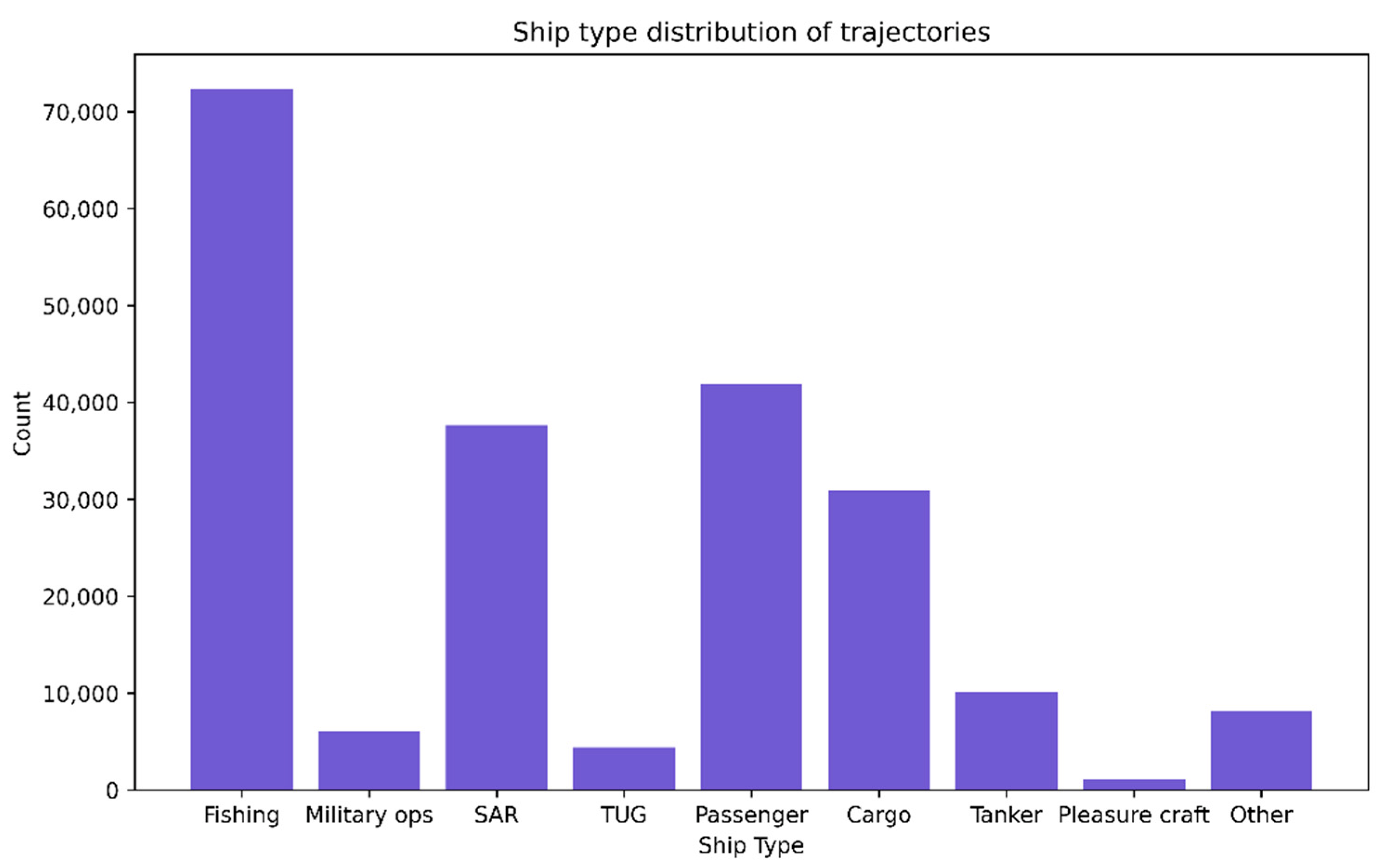
3.1. Data Preparing and Experimental Setup

A real-world maritime dataset is used to validate the proposed method. The European Automatic Identification System (AIS) dataset is a heterogeneous integrated dataset for maritime intelligence, surveillance and reconnaissance. It covers a time span of six months, from 1 October 2015 to 31 March 2016, and provides ships positions within the Celtic sea, the Channel and Bay of Biscay (France). There are 41 vessel types in the European AIS dataset with over 19 million AIS recordings. Nine vessel types from the European AIS data are chosen: Fishing, Military Ops, SAR (Search and Rescue), Tug, Passenger, Cargo, Tanker, Pleasure Craft and Other. The data points’ total number in each track is 30. Additionally, 80% of the dataset is divided into a training dataset and 20% is divided into a testing dataset, on which the following experiments are based.

The ship type distribution of trajectories is shown in Figure 3. The y-coordinate means the count of trajectories of each ship type. The abscissa means the ship types. There are a total of 212,508 trajectories in both the training dataset and testing dataset. The fishing type has 72,298 trajectories, which is the largest number among all ship types, while the pleasure craft only has 1060 trajectories. The number of trajectories of fishing, SAR, passenger and cargo is much higher than other ship types. The number of trajectories of different target types is not evenly distributed, which is consistent with most of the actual situation. As a data-driven method, the training of deep learning model requires plenty of samples to update the parameters of the model and learn the rules of dataset. Therefore, the dataset greatly affects the performance of the model. However, in the real world, data are always unevenly distributed. Only when the method can overcome the disadvantage of an uneven number of samples can it be meaningful to solve practical problems. Although the numbers of military ops, tug, tanker pleasure craft and other target types are much less than others, there are more than 1000 trajectories of each type, which are available to train the BTNN.

Figure 4 shows some examples of tracks of different ship types. The tracks are drawn by selecting longitude and latitude from the track information, and the shapes of tracks are displayed intuitively on the two-dimensional plane. Some tracks have similar shape characteristics while some are quite different. Specifically, the tracks of fishing ships are more tortuous, which are obviously different from other tracks. This means that the fishing ships change the course more frequently than other types of ships. The passenger ship, cargo ship and tanker ship usually travel long distances from one port to another, so their tracks are clearly directional. However, the distance between passenger ships’ track points is generally larger than that of cargo ships. These are some of the differences that can be directly observed. More advanced motion characteristics still need to be extract by the model. The deep learning model has advantages to extract the advanced features. There are many factors that affect the characteristics of a ship’s motion, such as the ship’s power system, displacement and navigation tasks. Thus, different types of ships have different motion characteristics, which will be reflected in the track information. The difference makes it possible to predict the type of ships using tracks information by the deep learning model.

All experiments are implemented under PyTorch deep learning framework on a 64-bit station with Ubuntu20.04.2, 16GB of RAM, 8 Intel(R) Core (TM) i7-9700 CPU and NVIDIA RTX 2080Ti.

3.2. Dimension Analysis and Choice

This section is aim at analyzing the influence of different dimensions of $d_1$ and $d_2$ on the identification accuracy. After the dimension analysis, the most suitable dimensions of $d_1$ and $d_2$ are chosen. The dimensions of encoder layer $d_1$ and final feature vector $d_2$ have great influence on the identification ability of BTNN. Dimensions that are too high may cause dimension redundancy, increasing network parameters and lengthen the training time, while those that are too low will lose track information. In this section, the identification accuracies under different values of $d_1\in [5,10,15,20]$ and $d_2\in [30,60,90,120,150,180,210]$ are compared (see

Table 1. The accuracy of target identification in training data and test data under different values of $d_1$ and $d_2$.

	${\mathit{d}}_2=30$		${\mathit{d}}_2=60$		${\mathit{d}}_2=90$		${\mathit{d}}_2=120$		${\mathit{d}}_2=150$		${\mathit{d}}_2=180$		${\mathit{d}}_{\mathbf{2}}=210$
	Train	Test	Train	Test	Train	Test	Train	Test	Train	Test	Train	Test	Train	Test
${\mathit{d}}_{\mathbf{1}}=\mathbf{5}$	0.3613	0.3402	0.8646	0.8657	0.9155	0.8791	0.9342	0.9046	0.9500	0.9130	0.9630	0.9160	0.9494	0.9076
${\mathit{d}}_{\mathbf{1}}=\mathbf{10}$	0.3625	0.3402	0.9131	0.8746	0.9321	0.8804	0.9669	0.9273	0.9675	0.9265	0.9747	0.9396	0.9592	0.9226
${\mathit{d}}_{\mathbf{1}}=\mathbf{15}$	0.3699	0.3402	0.9310	0.9007	0.9312	0.9020	0.9601	0.9199	0.9664	0.9240	0.9737	0.9351	0.9721	0.9354
${\mathit{d}}_{\mathbf{1}}=\mathbf{20}$	0.3670	0.3402	0.9005	0.8864	0.9604	0.9255	0.9661	0.9337	0.9699	0.9218	0.9744	0.9343	0.9636	0.9340

). There are 28 experiments at all. The accuracies of target identification in both training data and testing data are listed. The best values of $d_1$ and $d_2$ were chosen. Firstly, the results between training data and testing data are similar, which shows that the model does not overfit. The model has good generalization ability. Secondly, according to Table 1, high values of $d_1$ and $d_2$ make the BTNN perform better. When the value of either $d_1$ or $d_2$ increases, the identification accuracy also increases, especially when the values of $d_1$ and $d_2$ are low. This can be explained by the BTNN architecture. The track input contains only basic motion information (timestamp, latitude, longitude, speed and course). With a high dimension of the encoder layer, the multi-head-attention module in it can get the motion connections among track points better and the encoder module can extract more advanced motion features. There is a great similarity among tracks of different targets. Therefore, if the dimension of the final feature vector is low, interclass distances among tracks in the feature representation space are short. When the distance between different targets’ features is long, the targets are more available to be classified. With longer interclass distances, the features among different targets are more discriminative. Therefore, high values of $d_1$ and $d_2$ result in high identification accuracy. However, too high dimensions would contain redundant feature dimensions and have no obvious improvement on BTNN performance. With the accuracy under different values of $d_1$ and $d_2$ shown in Table 1, $d_1$ = 10 and $d_2$ = 180 are selected. The results show that the proposed method is effective.

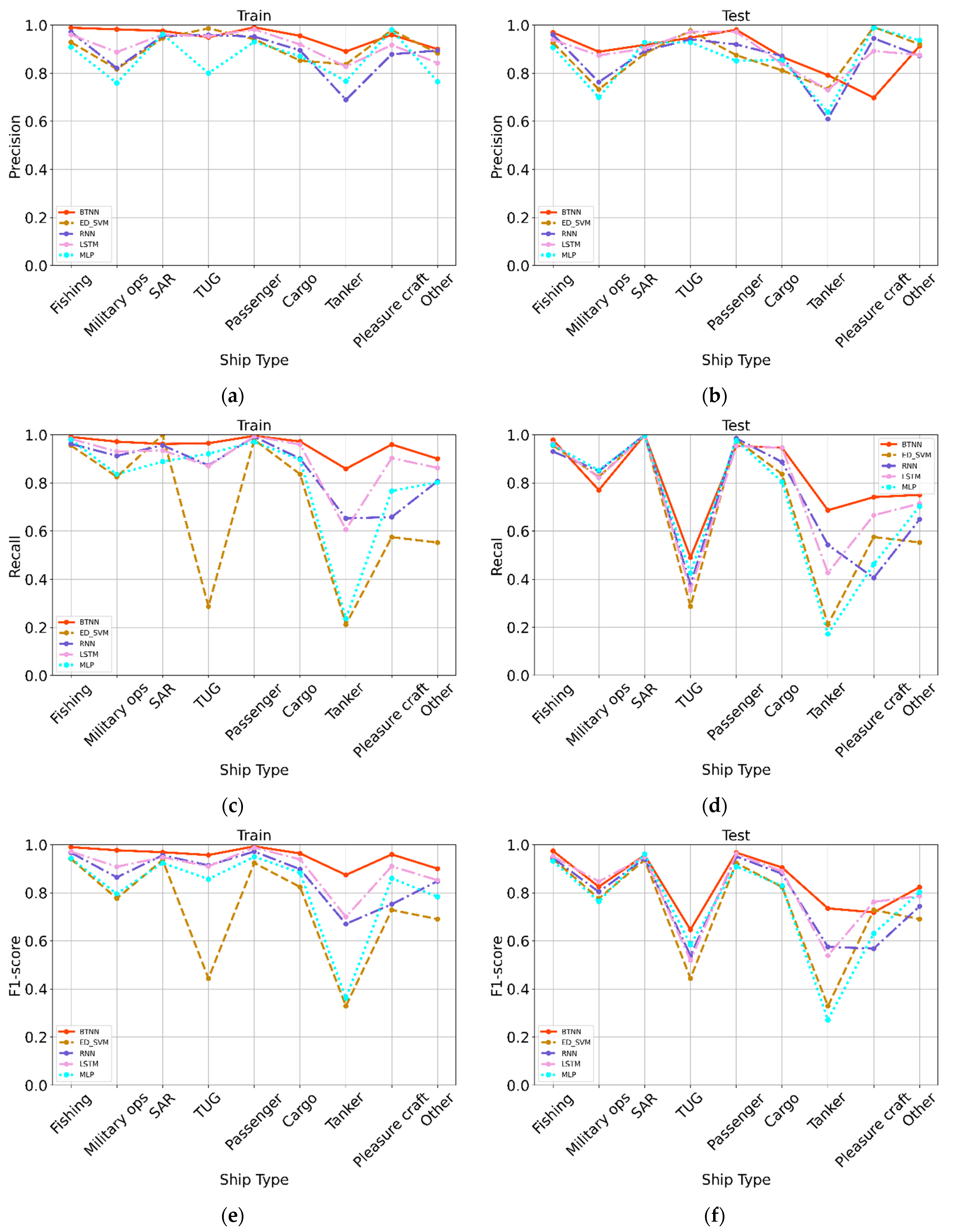
3.3. Accuracy Analysis and Comparison

In this section, the Precision, Recall and F1-score of the proposed method with results from ED_SVM [29], RNN [22], LSTM [19] and MLP [23] are compared. Precision, Recall and F1-scores are used to evaluate the dichotomous model which are defined as:

$$\mathrm{Precision}=\frac{TP}{TP+FP}$$

(15)

$$\mathrm{Recall}=\frac{TP}{TP+FN}$$

(16)

$$\mathrm{F}1-\mathrm{score}=\frac{2\times \mathrm{Precision}\times \mathrm{Recall}}{\mathrm{Precision}+\mathrm{Recall}}$$

(17)

where TP is the true positive, the number of positive samples that are correctly identified. FP is the false positive, the number of samples incorrectly identified as positive. FN is the false negative, the number of positive samples incorrectly identified as negative samples. F1-score evaluates the identification by combining Precision and Recall, and the closer to 1, the better BTNN deals with a multi classification problem.

Figure 5 demonstrates the results of class-level indicators, from which it can be observed that BTNN outperforms the ED_SVM [29], RNN [22], LSTM [19] and MLP [23]. The precision and recall of BTNN are higher than that of other methods in most target types. For the training set, the indicators of all target types that identified by BTNN are higher than 0.9 except the tanker target, while some of other methods’ indicators are lower than 0.8. The precision of tanker that identified by BTNN is 0.8903, the recall is 0.8586 and the F1-score is 0.8742, but those indicators of tanker that identified by other methods are far less than BTNN. For the testing set, the indicators of most target types are declined. However, compared with other method, the BTNN achieved better results. Although BTNN has a lower precision for pleasure craft than other methods, the F1-score is almost equal to others. Considering the recall and precision comprehensively, it can be concluded from the F1-score calculated by Equation (17) in Figure 5e,f that BTNN performs better than other methods in identifying each target type.

After the analysis of the identification results on the class-level, the overall performance of the methods is summarized on the

Table 2. The Precision, Recall and F1-score of target identification in training data and test data by different methods.

	Weighted Precision		Weighted Recall		Weighted F1-Score		Accuracy
	Train	Test	Train	Test	Train	Test	Train	Test
ED_SVM [29]	0.9154	0.8784	0.9170	0.8806	0.9084	0.8652	0.9355	0.8958
RNN [22]	0.9324	0.9014	0.9328	0.9016	0.9322	0.8968	0.9328	0.9016
LSTM [19]	0.9455	0.9107	0.9468	0.9124	0.9451	0.9053	0.9468	0.9124
MLP [23]	0.8988	0.8757	0.9016	0.8822	0.8925	0.8679	0.9016	0.8822
BTNN (ours)	0.9704	0.9303	0.9704	0.9313	0.9703	0.9282	0.9747	0.9396

. The statistical metrics used to evaluate the overall performance of methods are Weighted-Precision, Weighted-Recall and Weighted-F1-score, which are defined as:

$$\mathrm{Weighted}-\mathrm{Precision}={\displaystyle \sum _{i=1}^n{\omega }_i\times {\mathrm{Precision}}_i}$$

(18)

$$\mathrm{Weighted}-\mathrm{Recall}={\displaystyle \sum _{i=1}^n{\omega }_i\times {\mathrm{Recall}}_i}$$

(19)

$$\mathrm{Weighted}-\mathrm{F}1-\mathrm{score}={\displaystyle \sum _{i=1}^n{\omega }_i\times \mathrm{F}1-{\mathrm{score}}_i}$$

(20)

where ${\omega }_i$ represents the proportion of the $i$ target type in all samples, $n$ is the total number of target types. Precision, Recall and F1-score reflect the ability of methods to identify each target type. Weighted-Precision, Weighted-Recall and Weighted-F1-score can indicate the overall Precision, Recall and F1-score of methods. In addition, weighted scores take into account the imbalance of the number of target types. Thus, the Weighted-Precision, Weighted-Recall and Weighted-F1-score are used as overall evaluation indicator of methods. As shown in Table 2, the BTNN achieves higher values in each indicator than others, which indicates that BTNN performs better on overall identification. Although some indicators of BTNN on the class-level are similar to other methods, the weighted indicators of BTNN are apparently higher than other methods. The results show that the BTNN can extract the features more effectively, which could classify the tracks of different ship targets more accurately.

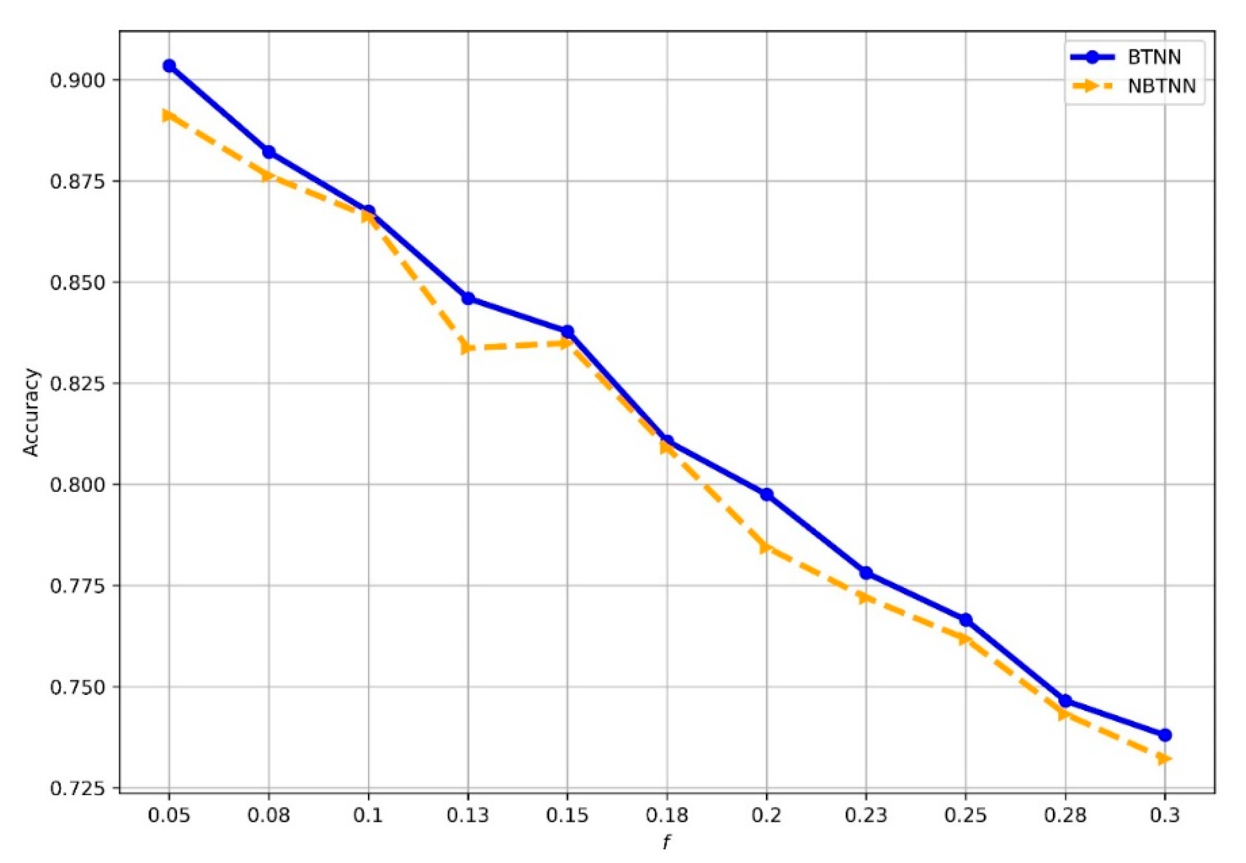
3.4. Network Anti-Noise Testing

In the real world, noise is everywhere, and so is the track data collected by different resources. In this section, the model is tested under different noise levels. Meanwhile, the BTNN is also compared with Non-Bayesian Transformer Neural Network (NBTNN) to show the improvement in the anti-noise ability of BTNN. Gaussian noise with a mean of 0 and standard deviation $f$ from 0.05 to 0.3 are added to the dataset, respectively. A larger number of $f$ indicates a higher level of noise. Figure 6 shows the result of the identification accuracy of BTNN and NBTNN under different values of $f$. Due to the noise, the motion characteristics of the tracks will not be obvious. As shown in Figure 6, the recognition accuracy remains above 0.75 for $f$ less than 0.28. It can be deduced that BTNN has a good anti-noise ability. In addition, when faced with noisy dataset, BTNN performs better than NBTNN, which shows that it is meaningful to apply Bayes’ principle in neural network. Furthermore, if the model misclassified the samples and the predictive probabilities are still high, the predictive probabilities are proved to be unreasonable. The samples that misclassified under a high-noise environment are selected to analyze their prediction probabilities. First, the probability values are equally divided into 10 segments with an interval length of 0.1, ranging from 0 to 1. Then, the number of misclassified samples are counted ($nu{m}_{ij},i\in [\mathrm{BTNN},\mathrm{NBTNN}]$) that fall into each interval $j$ and get the percentage of samples in each segment:

$${\mathrm{percentage}}_{ij}=\frac{nu{m}_{ij}}{nu{m}_i}\times 100\%$$

(21)

The results are presented in two bar charts in Figure 7a. Only 0.4% of the samples misclassified by BTNN have predictive probabilities greater than 0.9, but for NBTNN, the percentage was 3.5%. This means that NBTNN still provides exceptionally high predictive probabilities for the 3.5 percent of the misclassified samples. Moreover, the interval length of the segments is reset. In Figure 7b, the interval length is 0.2. In Figure 7c, the interval length is 0.5. Figure 7b shows that 2.3% of the samples misclassified by BTNN have predictive probability greater than 0.8; for NBTNN, the percentage is 13.2%. Figure 7c shows that 40.2% of the samples misclassified by BTNN have a predictive probability greater than 0.5; for NBTNN, the percentage is 59.2%. It can be concluded that most of the samples that are misclassified by BTNN have low predictive probabilities. In other words, the BTNN is not very confident about the classified results of these misclassified samples, which is significant for the commanders. Thus, for misclassified samples, the lower the predictive probabilities, the better the model performs. Compared with NBTNN, the samples that were misclassified by BTNN and have low predictive probabilities are more common. Thus, the BTNN performs better than NBTNN.

4. Discussion

To predict the type of the ship target, a Bayesian-Transformer Neural Network is proposed. The experiments above indicate that the proposed method performs well. The best values of dimension parameters are selected after the 28 experiments under different dimension parameters. The feature representation space is proved to be effective to classify the tracks of different target types. To demonstrate the generalization performance of the model, the testing dataset is set to test whether the model could identify the target using new track that does not appear in the training dataset. By analyzing the results of experiments, it can be seen that the accuracy of the training set and testing set are similar. It shows that the proposed model has good ability of generalization. The trained model can be used to identify the target using its track information.

By comparing the results of the proposed method with the ED_SVM [29], RNN [22], LSTM [19] and MLP [23], it can be concluded that the proposed method outperforms other methods. Firstly, the class-level experiments are implemented. The results show that the proposed method performs well in identifying each type of ship target. Meanwhile, the indicators of the proposed method are higher than others. Secondly, the overall ability of BTNN is compared with others. The results are shown in Table 2, which prove that the BTNN also outperforms other methods in terms of overall performance. The model can effectively extract features of tracks and classify the tracks in the feature space. However, there are also some shortages. For example, the BTNN is similar to other methods in its ability to identify some types of targets. Although the BTNN can identify the tug target more accurately than other methods, the recall for tug is still low, which means that many tug targets in the dataset are not being identified by BTNN.

The experiments of network anti-noise testing prove the efficiency of the application of the Bayes principle. The noise under different level is added to the data. The results show that the proposed method can maintain a high accuracy of identification and outperforms the Non-Bayesian Transformer Neural Network. In addition, most of the samples that are misclassified by BTNN have low predictive probabilities. Therefore, the BTNN could provide a more reliable predictive probability. On the contrary, the NBTNN has higher predictive probabilities for the misclassified targets, which means that the NBTNN is confident of the misclassified results. This will have serious consequences. The suspicious targets will thus evade supervision. In current studies, researchers tend to ignore this impact.

There are still some shortcomings that should be noticed. The proposed method is a data driven model with high requirements on the dataset. The neural network needs to learn the history data. Only after training with the history data can the model be used to identify targets of unknown types. Therefore, the accumulation of historical data and the establishment of datasets are also significant undertakings. In addition, the proposed method can only predict the type of the ship target. If the concrete information of the ship target is required, the BTNN will not be competent. Therefore, methods to combine the proposed method in this paper with the ways that identify the ship target by other information are one of the future focuses.

5. Conclusions

In this paper, a Bayesian-Transformer Neural Network (BTNN) is proposed to identify the ship target using tracks information. The tracks generated by ship target contain a wealth of features. Firstly, the discriminate features are extracted and another representation of the tracks is obtained using a Bayesian-Transformer Encoder (BTE) module. Then, a Bayesian fully connection layer and SoftMax complete the classification. BTNN belongs to the Bayesian Neural Network. The variational inference (VI) method is used to approximate the posterior distribution. In the experiments, the proposed method is evaluated on a publicly available dataset, Automatic Identification System (AIS). The experiments show that the proposed method can successfully identify nine types of ship targets. Compared with methods described in ED_SVM [29], RNN [22] and MLP [23], the identification accuracy of BTNN increased by 3.8% from 90.16%. The results of dimension analysis and choice demonstrate that the BTNN has a good generalization. In the class-level experiments, the proposed method achieves better indicators than other methods, which shows the efficiency of the method to identify each type of the ship target. The results of weighted-Precision, weighted-Recall and weighted-F1-score indicate that the BTNN also performs well in the overall level. In addition, the BTNN could provide a more reliable predictive probability under a high-noise environment. The anti-noise experiments show that the BTNN has a higher accuracy than NBTNN of identification under a noise environment. Meanwhile, the predictive probability provided by BTNN is more reliable than NBTNN, which proves that it is meaningful to apply Bayes’ principle in the neural network.

References

1. Guo, D.; Chen, B.; Chen, W.; Wang, C.; Zhou, M. Variational Temporal Deep Generative Model for Radar HRRP Target Recognition. IEEE Trans. Signal Process. 2020, 68, 5795–5809. [Google Scholar] [CrossRef]
2. Xu, C.; Yin, C.; Wang, D.; Han, W. Fast ship detection combining visual saliency and a cascade CNN in SAR images. IET Radar Sonar Navig. 2020, 14, 1879–1887. [Google Scholar] [CrossRef]
3. Ai, J.; Mao, Y.; Luo, Q.; Jia, L.; Xing, M. SAR Target Classification Using the Multikernel-Size Feature Fusion-Based Convolutional Neural Network. IEEE Trans. Geosci. Remote Sens. 2021, 60, 1–13. [Google Scholar] [CrossRef]
4. Bagnall, A.; Lines, J.; Hills, J.; Bostrom, A. Time-series classification with COTE: The collective of transformation-based ensembles. IEEE Trans. Knowl. Data Eng. 2015, 27, 2522–2535. [Google Scholar] [CrossRef]
5. Bagnall, A.; Lines, J.; Bostrom, A.; Large, J.; Keogh, E. The great time series classification bake off: A review and experimental evaluation of recent algorithmic advances. Data Min. Knowl. Discov. 2017, 31, 606–660. [Google Scholar] [CrossRef] [PubMed] [Green Version]
6. Lines, J.; Bagnall, A. Time series classification with ensembles of elastic distance measures. Data Min. Knowl. Discov. 2015, 29, 565–592. [Google Scholar] [CrossRef]
7. Hills, J.; Lines, J.; Baranauskas, E.; Mapp, J.; Bagnall, A. Classification of time series by shapelet transformation. Data Min. Knowl. Discov. 2013, 28, 851–881. [Google Scholar] [CrossRef] [Green Version]
8. Noyes, S.P. Track classification in a naval defence radar using fuzzy logic. In Proceedings of the Target Tracking & Data Fusion, Birmingham, UK, 9 June 1998. [Google Scholar]
9. Kouemou, G.; Opitz, F. Radar target classification in littoral environment with HMMs combined with a track based classifier. In Proceedings of the International Conference on Radar, Adelaide, Australia, 2–5 September 2008. [Google Scholar]
10. Doumerc, R.; Pannetier, B.; Moras, J.; Dezert, J.; Canevet, L. Track classification within wireless sensor network. In Proceedings of the SPIE Defense + Security, Anaheim, CA, USA, 4 May 2017. [Google Scholar]
11. Wang, Z.F.; Pan, Q.; Chen, L.P.; Liang, Y.; Yang, F. Tracks classification based on airway-track association for over-the-horizon radar. Syst. Eng. Electron. 2012, 34, 2018–2022. [Google Scholar]
12. Ghadaki, H.; Dizaji, R. Target track classification for airport surveillance radar (ASR). In Proceedings of the 2006 IEEE Conference on Radar, Verona, NY, USA, 24–27 April 2006. [Google Scholar]
13. Mohajerin, N.; Histon, J.; Dizaji, R.; Waslander, S.L. Feature extraction and radar track classification for detecting UAVs in civillian airspace. In Proceedings of the 2014 IEEE Radar Conference (RadarCon), Cincinnati, OH, USA, 19–23 May 2014. [Google Scholar]
14. Espindle, L.P.; Kochenderfer, M.J. Classification of primary radar tracks using Gaussian mixture models. IET Radar Sonar Navig. 2010, 3, 559–568. [Google Scholar] [CrossRef]
15. Sheng, K.; Liu, Z.; Zhou, D.; He, A.; Feng, C. Research on Ship Classification Based on Trajectory Features. J. Navig. 2017, 71, 100–116. [Google Scholar] [CrossRef]
16. Sarikaya, T.B.; Yumus, D.; Efe, M.; Soysal, G.; Kirubarajan, T. Track Based UAV Classification Using Surveillance Radars. In Proceedings of the 2019 22th International Conference on Information Fusion (FUSION), Ottawa, ON, Canada, 2–5 July 2019. [Google Scholar]
17. Zhan, W.; Yi, J.; Wan, X.; Rao, Y.J.I.S.J. Track-Feature-Based Target Classification in Passive Radar for Low-Altitude Airspace Surveillance. IEEE Sens. J. 2021, 21, 10017–10028. [Google Scholar] [CrossRef]
18. Fawaz, H.I.; Forestier, G.; Weber, J.; Idoumghar, L.; Muller, P.-A. Deep learning for time series classification: A review. Data Min. Knowl. Discov. 2019, 33, 917–963. [Google Scholar] [CrossRef] [Green Version]
19. Tan, H.X.; Aung, N.N.; Tian, J.; Chua, M.C.H.; Yang, Y.O. Time series classification using a modified LSTM approach from accelerometer-based data: A comparative study for gait cycle detection—ScienceDirect. Gait Posture 2019, 74, 128–134. [Google Scholar] [CrossRef] [PubMed]
20. Kooshan, S.; Fard, H.; Toroghi, R.M. Singer Identification by Vocal Parts Detection and Singer Classification Using LSTM Neural Networks. In Proceedings of the 2019 4th International Conference on Pattern Recognition and Image Analysis (IPRIA), Tehran, Iran, 6–7 March 2019. [Google Scholar]
21. Lai, C.; Zhou, S.; Trayanova, N.A. Optimal ECG-lead selection increases generalizability of deep learning on ECG abnormality classification. Philos. Trans. R. Soc. A 2021, 379, 20200258. [Google Scholar] [CrossRef] [PubMed]
22. Bakkegaard, S.; Blixenkrone-Moller, J.; Larsen, J.J.; Jochumsen, L. Target Classification Using Kinematic Data and a Recurrent Neural Network. In Proceedings of the 2018 19th International Radar Symposium (IRS), Bonn, Germany, 20–22 June 2018. [Google Scholar]
23. Ichimura, S.; Zhao, Q. Route-Based Ship Classification. In Proceedings of the 2019 IEEE 10th International Conference on Awareness Science and Technology (iCAST), Morioka, Japan, 23–25 October 2019. [Google Scholar]
24. Vaswani, A.; Shazeer, N.; Parmar, N.; Uszkoreit, J.; Jones, L.; Gomez, A.N.; Kaiser, Ł.; Polosukhin, I. Attention is all you need. In Proceedings of the Advances in Neural Information Processing Systems, Long Beach, CA, USA, 4–9 December 2017; pp. 5998–6008. [Google Scholar]
25. Jordan, M.I.; Ghahramani, Z.; Jaakkola, T.S.; Saul, L.K. An Introduction to Variational Methods for Graphical Models; Springer: Dordrecht, The Netherlands, 1998. [Google Scholar]
26. Kiureghian, A.D.; Ditlevsen, O. Aleatory or epistemic? Does it matter? Struct. Saf. 2009, 31, 105–112. [Google Scholar] [CrossRef]
27. Kingma, D.P.; Welling, M. Auto-Encoding Variational Bayes. In Proceedings of the ICLR, Banff, AB, Canada, 14–16 April 2014. [Google Scholar]
28. Dürr, O.; Sick, B.; Murina, E. Probabilistic Deep Learning; Michaels, M., Ed.; Manning Publications: Shelter Island, NY, USA, 2020; pp. 229–263. [Google Scholar]
29. De Vries, G.K.D.; Van Someren, M. Machine learning for vessel trajectories using compression, alignments and domain knowledge. Expert Syst. Appl. 2012, 39, 13426–13439. [Google Scholar] [CrossRef]
Figure 1. The structure of the BTNN.
Jmse 10 00577 g001
Figure 2. Multinomial distribution with nine target types: MN p 1 t T i , w t , , p k t T i , w t , , p 9 t T i , w t .
Jmse 10 00577 g002
Figure 3. Ship type distribution of trajectories.
Jmse 10 00577 g003
Figure 4. Examples of tracks of different ship types. (a) Fishing, (b) Military ops, (c) SAR, (d) TUG, (e) Passenger, (f) Cargo, (g) Tanker, (h) Pleasure Craft and (i) Other.
Jmse 10 00577 g004
Figure 5. Comparison of Precision, Recall, and F1-score values of different experimental schemes. (a) Precision of every target type on training dataset, (b) Precision of every target type on test dataset, (c) Recall of every target type on training dataset, (d) Recall of every target type on test dataset, (e) F1-score of every target type on training dataset and (f) F1-score of every target type on test dataset.
Jmse 10 00577 g005
Figure 6. Comparison of the performance under different f between BTNN and NBTNN.
Jmse 10 00577 g006
Figure 7. Comparison of percentage of misclassified samples in different predictive probability segments. (a) The interval of segments is 0.1. (b) The interval of segments is 0.2. (c) The interval of segments is 0.5.
Jmse 10 00577 g007