Subsoil Geological Structure Associations with Yield and Wine Attributes of Merlot Grapevines

Abstract

This study investigated the relationship between Subsoil Geological Structure (SSGS) and the yield, berry composition, and wine attributes of Merlot grapevines in a mountainous region. The research found significant differences in vine physiology, yield, and berry chemistry of grapevines between five adjacent rows, which corresponded with the underlying SSGS. The middle row, planted over filling material and a karst layer, had the highest yield (1.96 kg·vine⁻¹), consistent with better water availability, but produced berries and wine with the lowest concentrations of anthocyanins, phenolics, and soluble solids, resulting in the lowest wine quality score (82.33 points). In contrast, the northernmost row planted over bedrock had the lowest yield (0.12 kg·vine⁻¹), consistent with limited water availability, but produced highly concentrated berries, though extreme stress compromised overall wine balance. The southern row, positioned over filling material on bedrock with moderate water stress (stem water potential −1.4 MPa), achieved an optimal balance between yield and quality, producing wine with the highest sensory score (88.78 points) and favorable chemical composition. Geophysical methods, including electric resistivity tomography (ERT) and ground-penetrating radar (GPR), identified the subsurface structure, revealing the karst layer beneath high-yielding rows and consolidated bedrock beneath severely stressed rows. Chemical analyses of berries and wine confirmed the dilution effect of higher water availability on quality-determining compounds, providing mechanistic evidence linking SSGS to wine quality. This study demonstrates the utility of integrating geophysical, physiological, and enological approaches for understanding terroir effects and optimizing vineyard management in complex geological settings.

1. Introduction

Subsoil geological structure (SSGS) plays a fundamental role in grapevine growth and development, encompassing features such as effective topsoil depth to bedrock, fracture density and connectivity, karst cavities, permeability contrasts between soil layers, and lateral subsurface flow pathways. These geological characteristics work together to control the three-dimensional distribution and temporal dynamics of water, nutrients, and oxygen in the root zone. Consequently, understanding and managing SSGS has become increasingly important for optimizing both grape production and wine quality.

The importance of SSGS is particularly pronounced in mountainous vineyard regions, where geological complexity creates unique challenges. Topsoils in these environments are often thin or entirely absent, bedrock frequently lies exposed or at shallow depths, and centuries of terracing have created artificial soil–bedrock interfaces with highly variable characteristics [1]. Several aspects of the subsurface become especially critical for vine–water relations in these settings. Effective topsoil depth determines the volume of soil-stored water that roots can access. Beyond the topsoil layer, bedrock type and fracture networks control whether roots can penetrate deeper to tap moisture reserves in the substrate. In carbonate terrains, this dynamic becomes more complex; karst features such as dissolution cavities and enlarged fractures can create localized pockets where water accumulates. Terraced vineyards add another dimension to consider, as the texture, compaction, and depth of anthropogenic fill materials influence both infiltration rates and water retention capacity. Water movement is not limited to vertical flow, either. Lateral subsurface pathways along topsoil–bedrock interfaces or through fractured bedrock can redistribute moisture across the landscape. Together, these terroir conditions shape the drought stress patterns that vines experience [2,3], which ultimately connect to wine attributes and quality [4].

SSGS characteristics influence multiple dimensions of vine performance through interconnected mechanisms. Topsoil structure, depth, and the nature of underlying geology define the physical environment for root development, determining pore space, water-holding capacity, and drainage properties that support healthy root system establishment [5,6,7,8,9]. These same properties govern soil moisture dynamics and nutrient availability by influencing microbial activity and organic matter decomposition processes [10,11,12]. In terraced systems specifically, the interplay among fill material depth, underlying bedrock characteristics, and the presence of fracture networks or karst features creates complex three-dimensional patterns in water availability. These patterns remain hidden from surface observations yet critically influence vine water status and productivity.

Water and heat stress during the growing season represent major sources of variation in red wine yield and quality [13,14]. Recent studies have demonstrated strong linkages between soil water availability and grapevine physiological responses, including stomatal regulation and photosynthetic performance [15]. While extreme drought stress reduces grape yield, decreases berry size, and compromises wine quality [16], the relationship between stress and quality is not simply linear. Heat stress further modifies this dynamic by altering ripening trajectories, sugar accumulation patterns, acidity levels, and phenolic compound development [17,18]. Research on Merlot vineyards indicates that maintaining stem water potential above approximately −1.4 MPa produces optimal grape and wine quality [19,20]. For instance, the literature on deficit irrigation demonstrates that regimes delivering 50% of crop evapotranspiration during early berry development, then reducing to 20% during later stages, can successfully balance vegetative growth, yield, berry composition, and wine quality [19]. However, in the present study, all rows received uniform irrigation (35% ET_c), and the observed differences in vine water status arose solely from SSGS effects on water availability rather than differential irrigation treatments.

Understanding root-zone physical constraints has become increasingly critical in Mediterranean cropping systems facing climate variability. Recent comprehensive reviews emphasize that abiotic stressors, including elevated temperatures, increased vapor pressure deficits, water scarcity, and modified solar radiation, typically act simultaneously and often synergistically, challenging both crop productivity and resource management [21]. While controlled environment agriculture offers some buffering capacity, open-field viticulture remains directly exposed to external climatic forcing. In these systems, vine performance is strongly modulated by subsurface geological structure, particularly in mountainous Mediterranean terroirs where thin soils and exposed bedrock generate sharp spatial gradients in water availability and vine performance. Achieving optimal water stress levels becomes complicated when SSGS varies considerably over short distances, creating challenges for irrigation management—especially in new vineyard plots or terraced landscapes where the subsurface architecture remains poorly understood [22,23].

Before planting, developing an understanding of plot-scale soil–substrate–geology systems is essential. In practice, however, growers typically rely on geological surveys of exposed outcrops, existing soil maps, or local agronomic experience. When SSGS characteristics are poorly constrained, and vineyard performance exhibits pronounced spatial variability, geophysical methods can provide valuable explanations for the observed heterogeneity. Non-invasive geophysical techniques overcome many limitations of traditional invasive approaches while offering detailed insights into vineyard subsurface conditions, including variations in effective topsoil depth, bedrock depth and lithology, the presence of karst features or fracture zones, and spatial patterns in subsurface moisture dynamics [23,24].

By mapping SSGS heterogeneity, vineyard managers can delineate terrain-based management zones and implement targeted, site-specific adaptation strategies. Geophysical surveys excel at detecting and mapping features such as hidden bedrock cavities, fracture networks, and other structural elements that significantly influence vineyard development and long-term management [25,26,27]. Techniques such as electrical resistivity tomography (ERT) and ground-penetrating radar (GPR) enable detailed characterization of subsurface conditions, improving our understanding of vine–soil–substrate interactions and supporting the design of more precise management practices [28].

Despite the clear potential of these geophysical methods and the well-documented relationships between vine water stress and wine quality, important knowledge gaps remain. Most geophysical studies in viticulture have focused on vineyard planning and soil mapping, with few integrating geophysical characterization of SSGS with comprehensive physiological monitoring, berry chemistry, and wine quality outcomes within a single experimental framework. The specific mechanisms by which discrete geological features influence vine performance through altered water availability patterns are rarely documented with direct chemical evidence linking subsurface structure to berry composition and wine attributes. Furthermore, terraced vineyards, which represent a common viticultural practice in mountainous regions worldwide, present particularly complex SSGS scenarios due to anthropogenic modification of natural soil profiles, yet integrated geophysical–agronomic–enological studies in these systems remain scarce.

The present work addresses these gaps through a comprehensive interdisciplinary approach conducted within a single-terraced Merlot vineyard exhibiting spatial variability in vine performance despite uniform management. We combine non-invasive geophysical characterization of SSGS using both ERT and GPR to provide complementary information on subsurface structure and moisture dynamics, detailed physiological monitoring including stem water potential, gas exchange, and leaf area index, comprehensive berry and wine chemical analyses covering anthocyanins, phenolics, color parameters, and acidity, plus sensory evaluation. This integrated design allows us to trace mechanistic pathways from specific geological features through water availability and vine physiological responses to berry chemistry and ultimately wine quality, providing direct evidence for how SSGS influences terroir expression.

Based on hydrogeophysical principles and established plant–water relations, we developed specific expectations to guide our investigation. Regarding geophysical signatures, we anticipated that low electrical resistivity in ERT surveys combined with disrupted or weak GPR reflections in the upper 1–2 m would indicate high-porosity zones—such as unconsolidated fill, karst features, or fractured bedrock—with elevated water content. Conversely, high resistivity paired with continuous, strong horizontal GPR reflections should reflect consolidated bedrock with limited water storage capacity. We also expected seasonal resistivity contrasts between winter and summer surveys to be more pronounced in high-porosity zones, indicating greater moisture storage and buffering capacity.

From a physiological perspective, we expected vines positioned above geological features associated with higher water availability—low-resistivity zones, karst structures, or thick fill layers—to exhibit less negative stem water potential, indicating reduced water stress. These same vines should maintain higher stomatal conductance and net CO₂ assimilation rates, reflecting adequate water supply for photosynthetic activity. Greater vegetative growth should manifest as higher leaf area index and pruning mass, along with increased yield and potentially larger berry size.

Concerning wine quality relationships, we recognized that the connection between water availability and wine quality is non-linear, with moderate stress typically producing optimal results. We therefore expected that vines with excessive water availability would produce larger but more dilute berries with lower anthocyanin and phenolic concentrations, yielding wines with reduced color density, lower phenolic content, and diminished sensory quality scores. Vines experiencing moderate water stress around −1.4 MPa stem water potential for Merlot should achieve an optimal balance between yield and quality, producing concentrated berries and wines with high phenolic content, good color, and superior sensory scores. Under extreme water stress conditions (stem water potential more negative than −1.6 MPa), we anticipated declining wine quality despite high compound concentrations, due to impaired photosynthesis, accelerated ripening, potential off-flavor development, and wine imbalances such as elevated volatile acidity.

These expectations were formalized into specific testable hypotheses. We predicted that ERT and GPR surveys would reveal spatial variations in subsurface structure across our five study rows, with distinctive resistivity patterns and GPR reflection characteristics corresponding to differences in geological features such as fill depth, bedrock depth, and the presence of karst or fracture zones. These geophysical patterns should correspond spatially with vine water status measurements, with low-resistivity, high-porosity zones associated with less negative stem water potential and higher gas exchange rates, while high-resistivity, consolidated bedrock zones would correspond to more negative stem water potential and reduced photosynthetic activity.

We further hypothesized that these differential water stress patterns would translate into measurable differences in yield components and vegetative growth, with higher water availability supporting increased yield and more vigorous canopy development. Berry chemical composition at harvest should demonstrate an inverse relationship between water availability and concentrations of quality-determining compounds, with moderate stress producing optimal concentrations and extreme stress potentially compromising berry development. Wine chemical analyses should reflect these berry composition patterns, with wines from less stressed vines showing lower phenolic content and color density, wines from moderately stressed vines displaying optimal chemical profiles, and wines from extremely stressed vines potentially exhibiting signs of imbalance, such as elevated volatile acidity. Finally, sensory evaluation should assign the highest quality scores to wines from vines experiencing moderate water stress, with lower scores for wines from both excessively watered and extremely stressed vines.

By testing these mechanistic hypotheses in a terraced vineyard where adjacent rows exhibit contrasting performance under identical management, we aimed to demonstrate how non-invasive geophysical characterization of SSGS can explain terroir variability and inform precision viticulture management strategies.

2. Materials and Methods

2.1. Research Area

The study was conducted in a commercial vineyard in the 2021–2022 growing season in a small terrace plot of Vitis vinifera L. ‘Merlot’ grafted onto 140 Ruggeri rootstock; the vines were trained on a two-wire vertical shoot positioning (VSP) trellis system. Vines were planted in 2005 in a mountainous region (31.94° N, 35.12° E; elevation-441 m asl). Planting density was 3 m between rows and 1.5 m in rows (i.e., 2222.2 vines per hectare). The vineyard is situated on a steep terraced slope with approximately 15–20% gradient (8–11°) along the north–south axis. The five study rows are positioned on the uppermost terrace (horizontal platform created by cut-and-fill), with rows-oriented east–west (perpendicular to slope direction). The vines were irrigated twice a week using a computer-controlled drip irrigation system (Dream 1, Talgil, Kiryat Motzkin, Israel). The system was equipped with automatic valves and a mechanical flowmeter. A single line (20 mm) was used per row, with 0.5 m spacing and 2.4 L h⁻¹ in-line pressure-compensated drippers (Uni-ram, Netafim, Kibutz Hatzerim, Israel). Commercial irrigation practice was applied uniformly across all rows at 190 mm season⁻¹, equivalent to approximately 35% of the seasonal crop evapotranspiration (ET_c) estimated for red wine cultivars grown in the region [29].

The soil texture in the area is sandy loam composed of 56.4% sand, 26.6% silt, and 17% clay, with ample rocks present in the soil, and the plot was created as narrow terraces through cut-and-fill earthworks involving mechanical excavation, bedrock breaking, and redistribution of excavated material to create level planting platforms approximately 20 years ago; the grapevines were planted within the rock [29]. The vineyard plot was established in 2005 on a steep rocky slope through intensive terracing operations. The terraces were created by mechanical excavation and cut-and-fill earthworks. The composition and “filling material” shown consist of a disturbed mixture of excavated topsoil, weathered limestone fragments (2–20 cm diameter), and terra rossa (reddish clay-enriched soil derived from limestone weathering). The topsoil depth in the research plot is variable, from non-exposed bedrock to 40 cm in depth at most. The topsoil is discontinuous; depth varies spatially based on pre-existing bedrock topography and the extent of mechanical processing during terrace construction. Underlying bedrock is Cenomanian–Turonian limestone and dolomite (Judean Hills carbonate sequence) with documented karst weathering features [30]. The measurements were done on five rows with ten vines in each row. The climate is typically Mediterranean, characterized by hot, dry summers (June–September) and mild, wet winters (November–March). Based on regional climate data from the Israeli Meteorological Service for the region, the long-term (1981–2010) averages were: annual rainfall, ~550 mm; mean annual temperature, ~18 °C; summer (June–August) mean maximum temperature, ~31 °C; and winter (December–February) mean minimum temperature, ~8 °C. During the study period (2021), annual rainfall was approximately 480 mm (12% below average, representing a moderately dry year), with no rainfall between May and September.

Experimental Design and Statistical Considerations

This study employed an observational design investigating naturally occurring SSGS heterogeneity within a commercial vineyard plot. The five rows represent distinct geological units as characterized by geophysical methods (ERT and GPR), with each row positioned over a different subsurface configuration. Within each row, ten consecutive vines were measured to characterize row-level performance while accounting for residual within-row spatial variation. While each SSGS unit (row) lacks true spatial replication, a common constraint in terroir studies where geological features occur uniquely, the multiple vines per row serve as subsamples that improve the precision of row mean estimates and allow assessment of within-unit consistency and do not constitute pseudo replication in the classical sense [31]. Statistical comparisons among rows test whether SSGS-associated differences exceed the magnitude of within-row variation, providing evidence for SSGS effects under field conditions. The experimental unit for SSGS comparisons is the row (n = 5), while individual vines (n = 10 per row) serve as observational subunits. This hierarchical structure is typical of on-farm terroir characterization studies where geological features cannot be randomly assigned or replicated [24,32]. We acknowledge that the lack of true replication of SSGS types limits causal inference and generalization beyond this specific site. However, the strong concordance between geophysical characterization, physiological responses, yield components, and wine quality across rows provides converging evidence for SSGS influence on vine performance in this Mediterranean mountainous context. The findings should be interpreted as hypothesis-generating for future controlled studies rather than definitive proof of SSGS effects.

2.2. Phenology

There are three main stages in a grapevine’s development: the first stage is from fruit set to bunch closure, the second stage is from bunch closure to veraison, and the third and last stage is from veraison to harvest [33]. The phenological measurements were taken weekly and are summarized in

Table 1. Dates of phenological stages during the 2021 growing season in Dolev vineyard.

Beginning of the Phenological Stage	Date
Budburst	30 March 2021
Flowering	29 April 2021
Bunch closure	4 May 2021
Veraison	29 June 2021
Harvest	12 September 2021

.

2.3. Stem Water Potential (Ψ_s) Measurements

Physiological measurements and gas exchange were conducted on 50 experimental vines. To avoid potential bias associated with measurement timing, in each measurement row, the first five vines were measured initially, and only after completion of 25 measurements were the last five vines in each row. Ψ_s was measured three times during the growing season, once a month from June to August. Measurements were taken a day before the vineyard was irrigated at midday from 12:00 to 14:00, based on a standard method [34], using a cart-mounted portable pressure chamber (Arimad 3000, MRC, Holon, Israel). Measurements were done (one leaf per vine, ten vines per row, fifty vines in total) on mature, fully expanded, sun-exposed leaves covered with a plastic bag and an aluminum bag one and a half hours before the measurements started. Special attention was given to starting the measurement within 20 s of leaf detachment from the vine.

2.4. Leaf Area Index (LAI) Measurements

The leaf area index (LAI) indicates the leaf area (one side) per unit of ground surface area allocated for one vine [18,28]. During the growing seasons, the LAI values of all vines were calculated multiple times using a non-invasive canopy analysis system (SunScan model SS1-R3-BF3; Delta-T Devices, Cambridge, UK). The system employs a line quantum sensor array that detects photosynthetically active radiation (PAR) to estimate LAI through gap fraction inversion based on light measurements under the canopy. The manufacturer’s standard protocol was used to operate the analyzer. Each sample (measured vine) comprised readings evenly spaced at 20 cm intervals at ground level, starting from the center of the row and ending at half the distance to the adjacent row, with the linear probe parallel to the rows.

2.5. Gas Exchange

Leaf net CO₂ assimilation rate (An) and stomatal conductance (g_s) were measured using a portable infrared gas exchange system (model LI-6400, Li-Cor Biosciences, Lincoln, NE, USA) equipped with a standard leaf chamber. Measurements were performed at solar noon and on the day preceding irrigation, in order to minimize short-term variability associated with diurnal patterns and irrigation events. Gas exchange measurements were conducted under controlled chamber conditions, with photosynthetically active radiation set to a saturating light level (approximately 1000 µmol photons m⁻² s⁻¹), a reference CO₂ concentration representative of ambient conditions, and a constant air flow rate through the chamber. Measurements were carried out under prevailing ambient temperature and humidity conditions. Leaves selected for gas exchange measurements were of similar position and exposure to those used for stem water potential determinations. Before each measurement campaign, the instrument was calibrated and validated according to the manufacturer’s recommended procedures to ensure measurement accuracy and consistency.

2.6. Electric Resistivity Tomography (ERT) Measurements

The geophysical surveys were limited to five rows, approximately three meters apart, in the uppermost terrace of the vineyard, which exhibited visible differences among them, although receiving the same treatment. The ERT surveys were designed to characterize lateral and vertical variations in subsurface electrical resistivity as a proxy for lithological contrasts (consolidated bedrock vs. unconsolidated fill material), porosity differences, and spatial patterns in subsurface moisture distribution in the upper 2.5 m of the subsurface, the zone most relevant to grapevine root water access. The ERT surveys were conducted using a Wenner array configuration, with a high signal-to-noise ratio and high vertical sensitivity [35]. The surveys used a 20-electrode line with 1 m spacing between electrodes. The electrodes were placed near the vine trunks, where 10 central electrodes were placed near the vines used in this research, while the outer 5 electrodes on each side of the line were placed before and after the research area, in order to provide wide margins and to reduce edge effects. The 1 m electrode spacing was selected as a compromise between horizontal resolution and adequate penetration depth. With 20 electrodes spanning 19 m, this configuration provides: (1) sufficient lateral coverage to characterize the subsurface beneath all 10 study vines per row (located in the central 10 m portion of each line); (2) 5 guard electrodes positioned on each end to minimize edge effects in the inversion process; and (3) approximately 0.5 m horizontal resolution in inverted sections, matching the spatial scale of individual vine root zones (given the 1.5 m in-row vine spacing). This setting allows for reasonable horizontal resolution of half a meter per pixel in the resulting cross-section, fitting the problem requirements. A total line length of nineteen meters allowed a penetration depth of ~3 m [35]. Two field campaigns were conducted: in late summer (28 August 2021), representing minimum seasonal soil moisture, and in late winter (15 February 2022), representing maximum seasonal soil moisture following the rainy season. The investigation depth was deemed sufficient because: (1) grapevine roots in this relatively young (16-year-old) vineyard planted on shallow rocky soil are expected to concentrate in the upper 1–2 m [36]; (2) pilot hand auguring at several locations indicated bedrock refusal at <1 m depth in some areas; (3) achieving greater investigation depth would require wider electrode spacing (e.g., 2 m), which would sacrifice the horizontal resolution needed to discriminate between-row differences at the 3 m row spacing employed in this vineyard. Using the RES2DINV software (v5.0.2) a finite difference forward modeling method was used for the inversion process, and a standard least squares constraint was used to minimize the RMS error between the measured data and the calculated apparent resistivity. The Gauss–Newton method was used to solve the least squares equation [35].

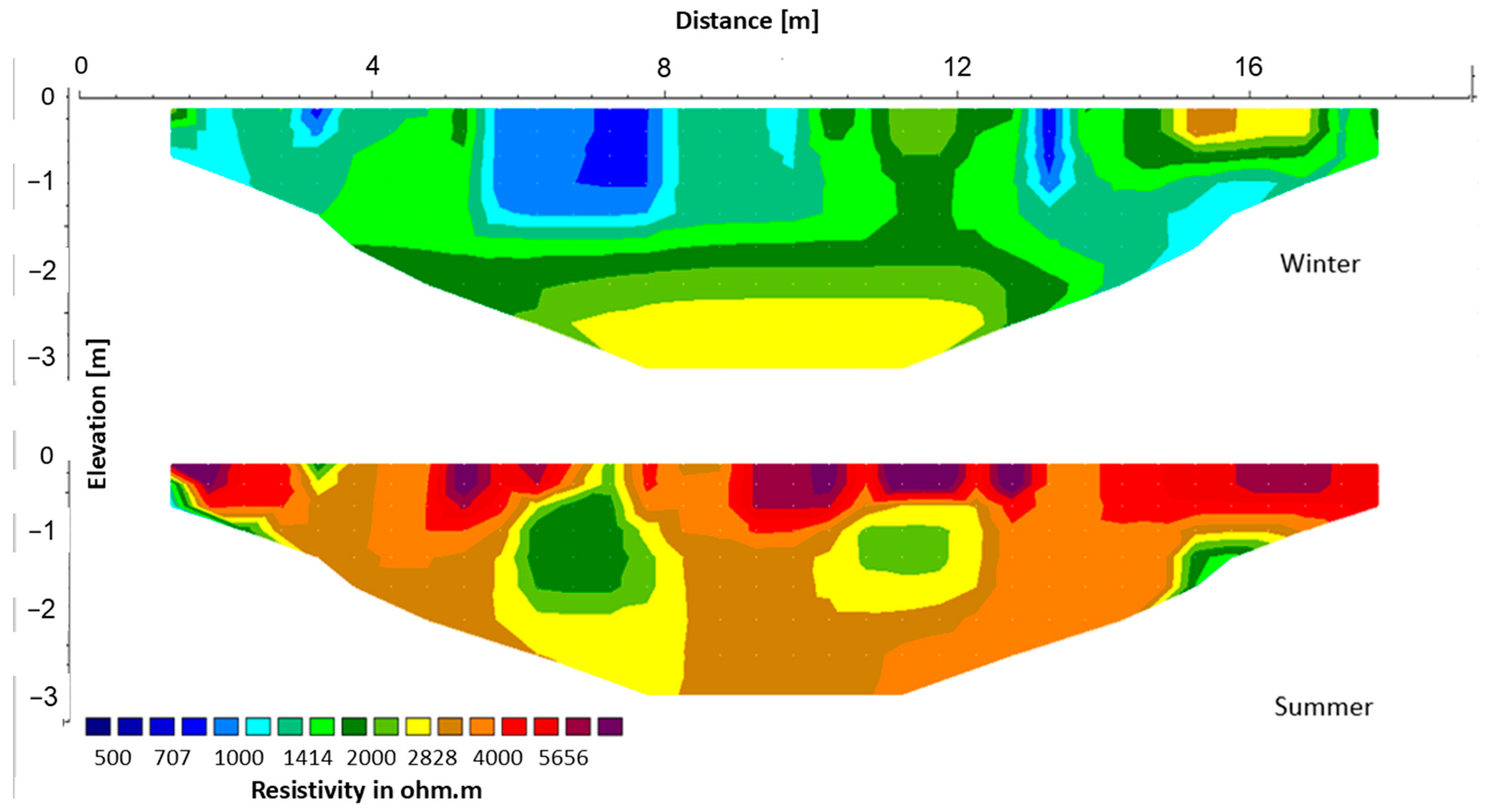
The ERT equipment for this setup consists of a 4-point light 10 W multi-channel portable earth resistivity meter system manufactured by Lippmann Geophysical Instruments. The system includes a 4-point light 10 W resistivity meter powered by a 12 V car battery and a row of twenty metal spike electrodes connected to an insulated low-resistance multi-core cable. The ERT data is later loaded into the RES2DINV software (v5.0.2) for apparent resistivity inversion to obtain the true resistivity of the subsurface. Inverted ERT profiles with depths and a standard resistivity rainbow scale are presented in Figure 1. The very-low-resistivity areas, indicated by blue–green colors, correspond to low resistive areas. Green–purple colors indicate high resistivity zones.

2.7. Ground-Penetrating Radar (GPR) Measurements

In addition, we surveyed eight GPR lines using a 250 MHz antenna. In order to ease comparing between the different methods, the GPR cross-section boundaries were set to nineteen meters long, and the 250 MHz antenna was chosen because the signal penetrates deeper than the 500 MHz, resulting in a much more meaningful penetration depth (2.5 m) while sacrificing resolution. For processing, we reversed the even number lines in order to present all results in the same direction. GPR data were collected using a Mala X3M system between the vines. The system consists of an antenna with a central frequency of 250 MHz dragged or rolled on a cart along a straight line (the distance is automatically measured), a controller connected to a computer with Mala’s Ground-Vision software (v2.1) installed, and a power source. The GPR data were loaded into Reflexw software (v9.5.8) for analysis, processing, and interpretation.

All GPR profiles were processed using the same flow and converted into depth scales using an average electromagnetic wave velocity of 0.1 m/ns, corresponding to typical values for dry, rocky soils with low clay content and low moisture (upper end of the typical 0.05–0.1 m/ns range), appropriate for the shallow soil profile over limestone bedrock at our site. A de-wowing filter was applied to remove low-frequency static noise, followed by a static correction to remove the effects at the contact between the antenna and the ground surface. A background removal filter was then applied to remove horizontal reflections, and a bandpass filter was used to remove unrelated frequencies. A divergence compensation gain function was applied to emphasize the critical differences between the consolidated and unconsolidated lines. Finally, a migration was performed to focus the radargram.

Geophysical Interpretation and Ground-Truthing

Interpretation of ERT resistivity and GPR reflectivity patterns was constrained by:

The site exhibits extensive bedrock outcropping at terrace edges and the upslope boundary, confirming shallow bedrock occurrence within the survey area. Rock fragments (predominantly limestone) dominate the surface layer across all rows.

According to the vineyard manager, the plot was mainly solid bedrock during planting preparation (2005), requiring mechanical excavation. The site is located within the Judean Hills carbonate sequence, characterized by Cenomanian–Turonian limestone and dolomite formations with documented karstic weathering features [30]. Karstification is common in this geological setting, creating subsurface cavities and fissure systems that can be partially or fully infilled with terra rossa soils and weathered rock debris. The resistivity values observed in this study align with published ranges for similar Mediterranean carbonate terrains: Compact limestone/dolomite bedrock—1000–10,000 ohm·m [37], Saturated soil/weathered rock—100–1000 ohm·m [38], Water-filled karst cavities—10–500 ohm·m [39]. Our observed values (500 ohm·m for inferred karst/filling vs. 4000 ohm·m for consolidated bedrock) fall within these documented ranges and are consistent with field observations and historical information. We acknowledge that systematic ground-truthing (e.g., continuous soil moisture monitoring, drilling cores, or trenching) was not conducted, limiting our ability to quantitatively validate geophysical interpretations. The subsurface model should be considered a qualitative conceptual representation based on geophysical signatures, field observations, and regional geological context rather than directly measured stratigraphy. However, the strong concordance between inferred SSGS heterogeneity and observed vine physiological responses, yield patterns, and wine quality supports the validity of the geophysical interpretation for this application.

2.8. Yield, Grape Must, Wine Chemical Analysis and Sensory Evaluation

2.8.1. Yield Measurements

Total yield per vine: All grape clusters were harvested from each of the 10 study vines per row and weighed immediately in the field using a portable digital scale (precision ± 1 g). The number of bunches per vine was counted directly during harvest. Bunch weight was calculated as the total yield divided by the number of bunches. The 100-berry weight was measured by taking three randomly selected, representative clusters per vine and 100 berries were sampled, weighed collectively, and the average was calculated. Berries per cluster were calculated from bunch weight and 100-berry weight. The pruning mass was measured by collecting wood canes from each vine and weighing them. Stem width was measured 10 cm above the graft union using digital calipers (precision ± 0.1 mm).

2.8.2. Must Analysis at Harvest

Berry samples were collected at harvest from each row for chemical analysis. Total soluble solids (TSS, °Brix) were measured using a digital refractometer. Must pH was determined using a calibrated pH meter. Berry skin anthocyanins and total phenolics were extracted and quantified following established protocols. For anthocyanin analysis, berry skins were macerated in acidified methanol solution, and total anthocyanins were determined spectrophotometrically at 520 nm. Results are expressed as mg anthocyanin per gram of berry fresh weight. For total phenolics, berry extracts were analyzed spectrophotometrically at 280 nm, with results expressed as absorbance units (0.01 AU per gram berry fresh weight). It should be noted that Row E reached physiological maturity approximately one week earlier than the other rows due to severe water stress and was harvested separately to prevent over-ripening and quality degradation.

2.8.3. Wine Chemical Analysis

Following fermentation, stabilization, and aging, wines from each row were analyzed for standard enological parameters. Residual sugars (glucose + fructose) were determined enzymatically and expressed as g/L. Total acidity was measured by titration and expressed as g/L tartaric acid equivalents. Wine pH was measured using a calibrated pH meter. Ethanol content (% v/v) was determined by distillation. Malic acid concentration was quantified enzymatically and expressed as g/L. Volatile acidity (VA) was determined by steam distillation and expressed as g/L acetic acid equivalents. Wine density was measured at 20 °C and expressed as g/L. Color parameters and phenolic content were assessed spectrophotometrically. Absorbance was measured at 420 nm (yellow pigments), 520 nm (red pigments), and 620 nm (blue pigments), with results expressed in absorbance units (AU). Color density (CD) was calculated as the sum of absorbances at 420, 520, and 620 nm. Color hue (CH) was calculated as the ratio of absorbance at 420 nm to 520 nm. Total phenolic content was determined by measuring absorbance at 280 nm after appropriate dilution, with results expressed in AU. All chemical analyses were performed according to standard enological methods [40].

2.8.4. Wine Sensory Evaluation

Following stabilization and an initial aging period, the wines were subjected to blind sensory evaluation. The assessment was carried out by a panel of nine professional oenologists with recognized expertise in wine tasting and extensive experience in evaluating red wines from the region. A total of five wines were evaluated, comprising one wine from each of the five experimental rows (A–E). The tasting was conducted in a single flight under controlled conditions (temperature 18–20 °C, natural lighting). Sample order was randomized to minimize order effects, and each wine was presented in identical, coded black glasses to ensure complete blinding. The sensory analysis followed a structured protocol based on the guidelines of the International Organisation of Vine and Wine for dry red wines [40]. The overall sensory score was calculated on a 100-point scale, integrating multiple attributes across visual, olfactory, and gustatory dimensions. Visual assessment included color quality (maximum 5 points) and color intensity (maximum 10 points); olfactory evaluation encompassed aroma concentration (maximum 8 points), aroma originality (maximum 5 points), and aroma quality (maximum 15 points); gustatory assessment addressed taste concentration (maximum 8 points), taste originality (maximum 5 points), taste quality (maximum 20 points), and aftertaste persistence (maximum 8 points); and an overall harmony score (maximum 10 points) reflected the balance and integration of sensory components. The sum of these individual scores yielded the total score out of 100 points.

2.9. Statistical Analysis

The data were analyzed using ANOVA, and the means were differentiated based on the least significant difference (LSD) at a significance level of p ≤ 0.05. All statistical analyses were carried out using the software program JMP PRO 16 (SAS Institute, Cary, NC, USA). Different letters in English mark statistical significance. Each vine in each row served as replicates (n = 10). Physiological measurements conducted on multiple dates (stem water potential, LAI, and gas exchange) were analyzed using separate one-way ANOVAs for each measurement date, testing for row effects at each individual time point. This approach characterizes row differences at discrete phenological stages (corresponding to key moments in berry development: post-fruit set, mid-berry growth, and pre-harvest) rather than modeling temporal trajectories or formally testing time × row interaction effects. We acknowledge that this analytical strategy does not account for temporal autocorrelation in repeated measurements on the same vines and cannot test whether rates of change differ among rows, representing a limitation of our statistical approach.

3. Results

All rows were found to be significantly different from each other (p < 0.0001) except for stem water potential on 19 August, where there was no difference between the rows (

Table 2. Midday LAI and stem water potential during the 2021 growing season, Merlot Dolev vineyard. Values represent means (n = 10). LAI—Leaf area index; ψ_s—stem water potential. Lower case letters indicate statistical group parsing.

Row	LAI [m2·m−2]			ψs [MPa]
Date	10 June	15 July	19 August	10 June	15 July	19 August
A	0.59 a	1.28 a	1.09 a	−0.56 a	−1.41 bc	−1.86 a
B	0.57 ab	1.09 b	1.08 a	−0.59 a	−1.33 b	−1.80 a
C	0.48 b	1.21 ab	1.23 a	−0.67 ab	−1.20 a	−1.46 a
D	0.32 c	0.69 c	0.72 b	−0.74 b	−1.50 d	−1.74 a
E	0.15 d	0.39 d	0.43 c	−0.76 b	−1.50 cd	−1.68 a
p-value	<0.0001	<0.0001	<0.0001	<0.0001	<0.0001	0.0835

).

The stomatal conductance measurements show an identical pattern on the dates (

Table 3. Midday net CO₂ assimilation rate and stomatal conductance during the 2021 growing season, Merlot Dolev vineyard. A_n—leaf net CO₂ assimilation rate; g_s—stomatal conductance. Values represent means (n = 10). Lower case letters indicate statistical group parsing.

Row	An [μmol/(m2·s)]			gs [mmol/(m2·s)]
Date	10 June	15 July	19 August	10 June	15 July	19 August
A	12.37 a	1.62 b	2.41 b	211.53 a	23.20 b	13.14 b
B	12.76 a	3.89 b	3.87 ab	217.96 a	53.90 b	23.97 ab
C	13.07 a	8.87 a	4.69 a	234.02 a	146.57 a	47.58 a
D	12.38 a	2.30 b	2.78 b	212.66 a	28.66 b	18.03 b
E	12.42 a	1.88 b	2.10 b	201.39 a	22.95 b	5.20 b
p-value	0.8995	<0.0001	0.0011	0.8286	<0.0001	0.0015

). A significant difference was found in the leaf net CO₂ assimilation rate on 15/07, when all rows were grouped except for row C, which consistently had higher values (Table 3). On 19 August, the pattern changed a little, with row B assigned to both groups.

A significant difference was found in yield components and pruning mass in every category, with a mixed pattern between each category (

Table 4. Yield components and pruning mass at the Dolev vineyard during 2021. Lower case letters indicate statistical group parsing.

Row	Yield (kg·Vine−1)	Bunch (Number·Vine−1)	100 Berry wt (gr)	# Berries per Cluster	Bunch wt (gr)	Pruning Mass (kg·Vine−1)	Canes (Number·Vine−1)	Stem Width (mm)
A	0.88 b	23.6 b	76.5 b	46.09 ab	37.28 b	0.47 a	29 ab	33.47 a
B	1.10 b	27.3 ab	78.6 b	54.89 a	40.29 b	0.60 a	30 ab	35.47 a
C	1.96 a	41.1 a	124.3 a	40.16 b	47.69 a	0.54 a	30.8 a	37.97 a
D	0.89 b	27.0 ab	92.3 b	40.47 b	32.96 b	0.25 b	27.3 ab	25.96 b
E	0.12 c	5.1 c	89.0 b	20.98 c	23.53 c	0.10 b	23.1 b	21.55 b
p-value	<0.0001	<0.0001	<0.0001	<0.0001	<0.0001	<0.0001	0.0472	<0.0001

). Interestingly, rows D and E were clustered together in stem width and pruning mass and were low compared to the other rows. Row E consistently had the lowest values throughout, except for 100-berry weight. Row C had consistently higher values in all categories except for the number of berries and pruning mass (Table 4).

Grape Must Composition, Wine Chemical Parameters

Significant differences in must composition at harvest reflected the varying water status and yield among rows (

Table 5. Must composition at harvest, Merlot Dolev vineyard, 2021. Lower case letters indicate statistical group parsing.

Row	TSS (°Brix)	pH	Anthocyanins (mg/g Berry)	Total Phenolics (AU/g Berry) *
A	25.2 a	3.64 ab	3.89 b	7.22 b
B	24.9 ab	3.65 ab	4.61 a	8.50 a
C	22.8 c	3.57 b	3.13 c	5.55 c
D	23.4 bc	3.72 a	3.95 b	7.02 b
E	26.1 a†	3.73 a	2.88 c	5.50 c
p-value	<0.0001	0.0023	<0.0001	<0.0001

* AU = absorbance units (0.01 AU per gram berry fresh weight at 280 nm). Different letters indicate significant differences (LSD, p ≤ 0.05). † Row E was harvested approximately one week earlier than other rows due to accelerated ripening under severe water stress.

). Total soluble solids (TSS) ranged from 22.8 °Brix in Row C to 26.1 °Brix in Row E (p < 0.0001). Row C, with the highest yield and lowest water stress, exhibited significantly lower Brix compared to all other rows. Conversely, Row E, harvested one week earlier due to accelerated ripening under severe stress, showed the highest Brix. Rows A, B, and D displayed intermediate values (23.4–25.2 °Brix). Must pH varied significantly among rows (p = 0.0023), ranging from 3.57 in Row C to 3.73 in Row E. Berry anthocyanin content showed significant variation (p < 0.0001), with Row B exhibiting the highest concentration (4.61 mg/g), while Row E had the lowest (2.88 mg/g). Row C showed relatively low anthocyanin content (3.13 mg/g) compared to Rows A, B, and D. Total phenolics in berry extracts followed a similar pattern (p < 0.0001), with Row B showing the highest values (8.50 AU/g) and Rows C and E the lowest (5.55 and 5.50 AU/g, respectively). Rows A and D exhibited intermediate phenolic levels (7.22 and 7.02 AU/g, respectively).

Table 6. Wine chemical parameters and color analysis, Merlot Dolev vineyard, 2021. Lower case letters indicate statistical group parsing.

Row	Ethanol (% v/v)	Total Acid (g/L TA)	pH	VA (g/L AA)	Yellow (AU 420 nm)	Red (AU 520 nm)	Blue (AU 620 nm)	CD (AU)	CH	Total Phenolics (AU 280 nm)
A	14.8 a	6.7 a	3.60 c	0.45 b	3.44 b	4.72 b	1.05 b	9.2 b	0.73 ab	49.6 b
B	15.2 a	5.9 ab	3.75 a	0.51 b	3.79 ab	5.10 b	1.26 ab	10.2 ab	0.74 ab	51.6 b
C	13.3 b	5.2 c	3.73 ab	0.49 b	2.56 c	3.28 c	0.79 c	6.6 c	0.78 a	43.7 c
D	12.3 c	5.1 c	3.65 bc	0.53 b	3.06 bc	4.45 b	1.02 b	8.5 b	0.69 b	52.4 b
E	13.4 b	6.4 ab	3.62 c	0.71 a	3.83 a	5.82 a	1.37 a	11.0 a	0.66 b	55.3 a
p-value	<0.0001	<0.0001	0.0156	0.0008	0.0002	<0.0001	<0.0001	<0.0001	0.0421	<0.0001

TA = tartaric acid equivalents; AA = acetic acid equivalents; VA = volatile acidity; AU = absorbance units; CD = color density; CH = color hue. Different letters indicate significant differences (LSD, p ≤ 0.05). Values represent means (n = 1 wine per row).

shows the significant differences among rows A–E in several chemical and color related wine parameters. Ethanol content was highest in rows A and B and lowest in D, indicating differences in fermentation performance. Rows C and D exhibited lower total acidity compared to the other rows. Volatile acidity was significantly higher in row E, suggesting altered microbial or metabolic activity. Absorbance values at 420, 520, and 620 nm differed significantly among rows. Row E had the highest color density (CD) and higher absorbance across all wavelengths. Total phenolic content followed a similar trend, with the highest values observed in row E and the lowest in row C. Color hue (CH) showed moderate but statistically significant variation among rows. Overall, row E resulted in wines with enhanced phenolic content and color intensity, whereas row C was characterized by generally lower values across most measured parameters.

The total results of the wine testing indicated that row C had the lowest score, indicating that the wine produced was of the lowest quality compared to the other rows (

Table 7. Wine tasting results. Each value is an average of 9 tasters (n = 9). cv. Merlot, Dolev vineyard, 2021. Lower case letters indicate statistical group parsing.

Row	Color Quality	Color Intensity	Scent-Concentration	Scent Originality	Scent Quality	Taste Concentration	Taste Originality	Taste Quality	Taste Aftertaste	General Assessment	Total
A	4.78 a	9.33 a	7.33 a	4.78 a	14.00 a	7.11 a	5.11 a	19.33 a	7.00 a	10.00 a	88.78 a
B	4.50 ab	9.00 a	7.00 a	4.88 a	14.50 a	7.38 a	5.13 a	18.63 a	7.25 a	10.13 a	88.38 a
C	4.00 b	7.11 b	6.78 a	4.89 a	13.78 a	6.56 a	4.78 a	17.67 a	6.89 a	9.89 a	82.33 b
D	4.67 ab	8.89 a	7.00 a	5.00 a	13.78 a	6.89 a	4.89 a	19.00 a	6.67 a	9.89 a	86.67 a
E	4.44 ab	9.33 a	6.89 a	4.67 a	13.56 a	7.22 a	4.89 a	17.67 a	6.78 a	10.22 a	85.67 ab
p-value	0.0233	0.0002	0.3941	0.5607	0.3315	0.1525	0.3632	0.0402	0.1025	0.5741	0.0004

). Row E ranked the second lowest, but closer to row D than row C (Table 7).

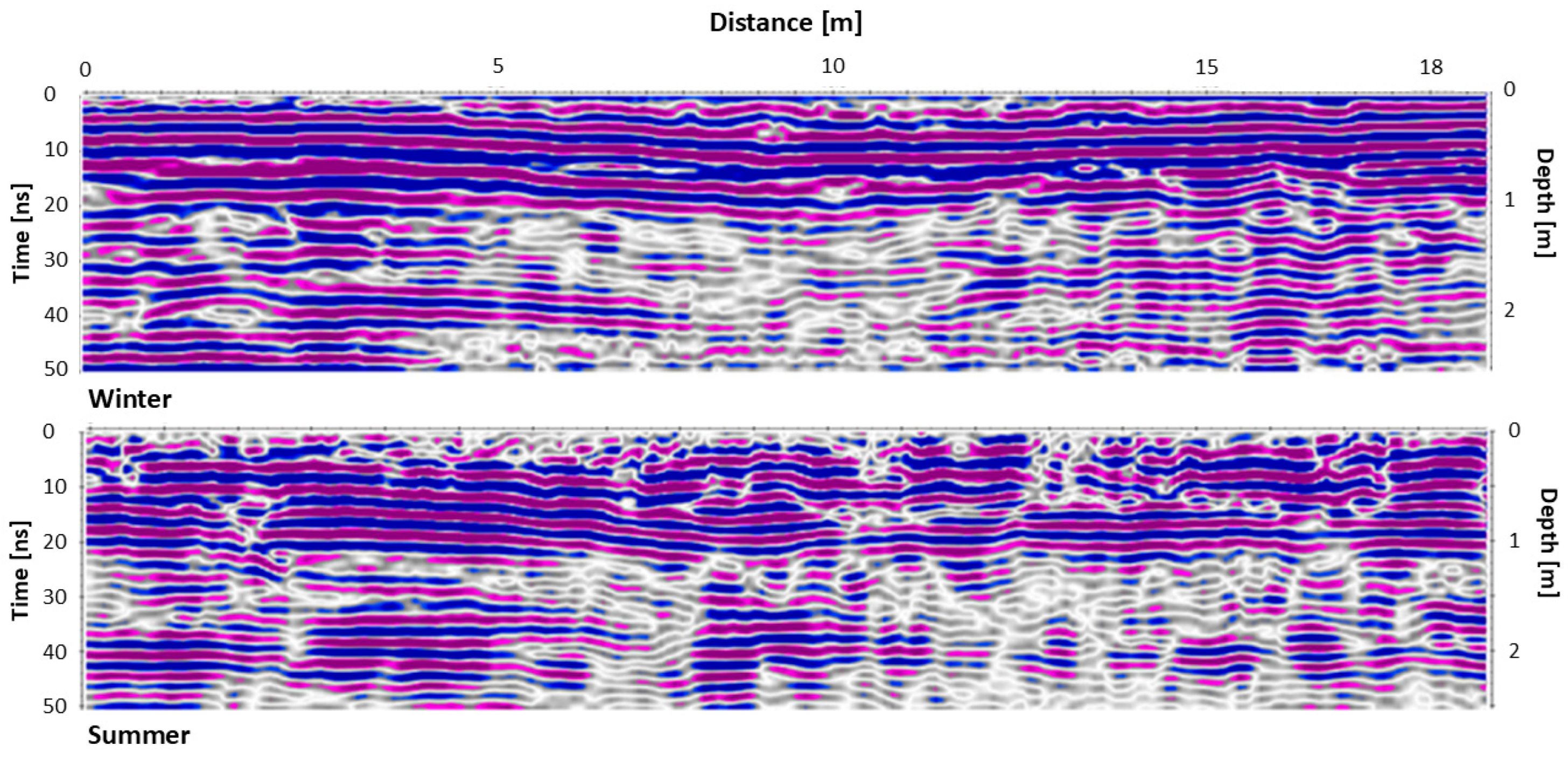
Inverted line ERT3 (Figure 1) and processed line GPR5 (Figure 2) were chosen for comparison between the water content in the ground during the summer (higher in the figure) and winter (lower in the figure) seasons. In ERT, areas fully or partially filled with materials with high porosity (cavities filled with unconsolidated rocks and fine, moist soil) are expressed as areas of low resistivity, 500 ohm.m [41]. High-resistivity (4000 ohm.m) anomalies indicate consolidated bedrock. With the GPR method, a higher soil moisture level may increase the wave decay rate, increase clutter, and make the target harder to resolve [42]. GPR shows that the upper layer under line GPR5 is unconsolidated sediments, in contrast to line GPR1, which has continuous horizontal reflections indicating consolidated bedrock (Figure 2). Although quantitative analysis of water content without calibrating site-specific petrophysical relations is restricted, it can be claimed that both methods show a clear difference in moisture amount in the subsoil between the seasons. For example, by assuming an Archie’s petrophysical model [43] with typical parameters of a saturation exponent of 2 and formation factor of 0.1 [44], and pore-water EC of 1 dS/m (irrigation water EC), it can be evaluated that water saturation is reduced by 30% between seasons at the top 1.5 m, while only a 5% decrease in water saturation can be evaluated below that depth. Such an observation can imply that the subsoil has a large porosity and absorbs water easily during rainy days. However, the moisture quickly penetrates great depths, and the upper layers do not retain moisture and dry out completely by summer.

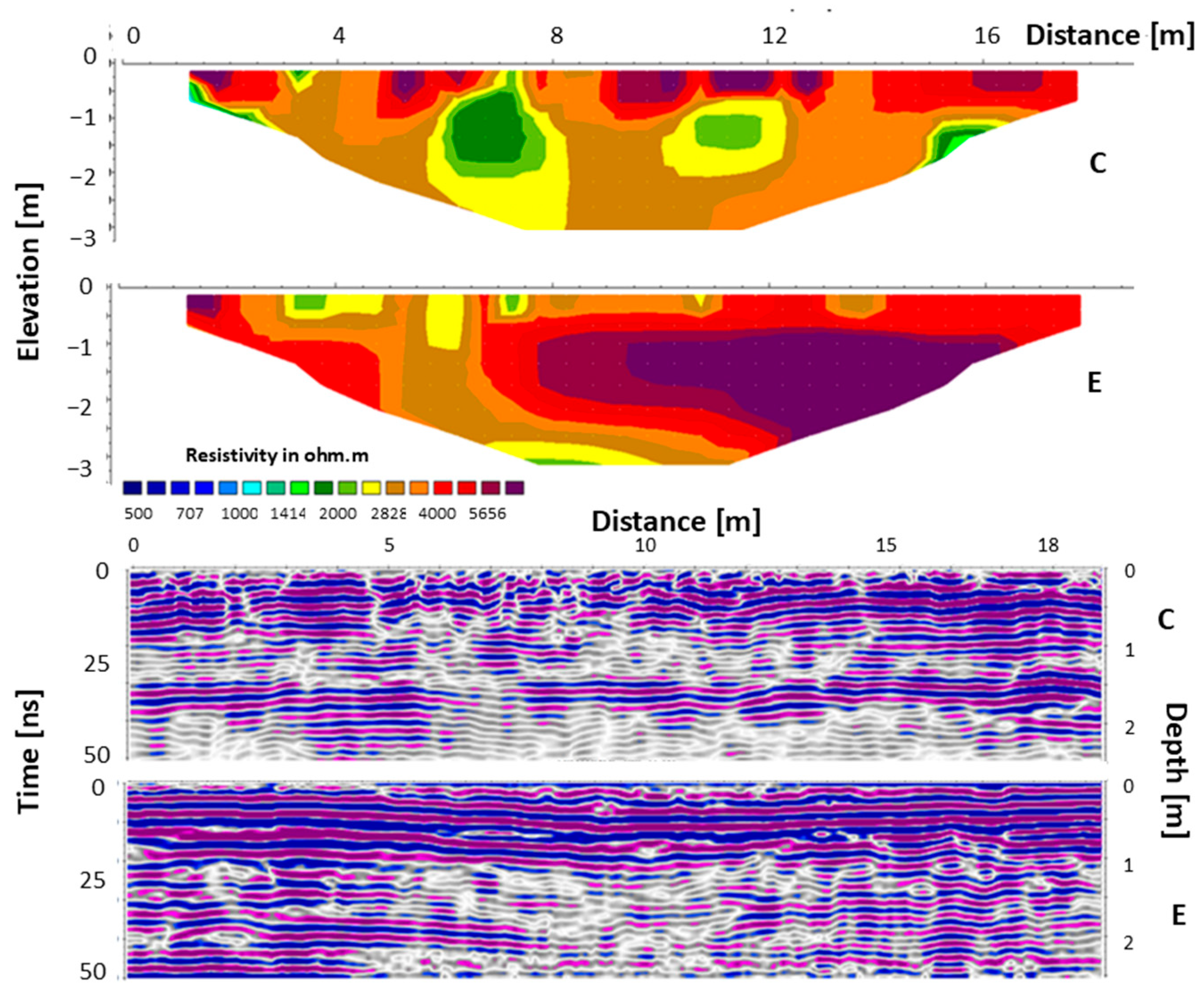
Another comparison was made with both methods between the best-growing row C (represented by lines ERT3 and GPR5) and the worst-growing row E (represented by lines ERT1 and GPR1) in winter (Figure 3). The differences between the two lines can be seen more clearly with both methods. In line C, the upper layer contains soil with rocks up to a depth of about one meter, followed by a deeper rock layer, which probably retains moisture close to the roots of the plants and allows them to grow well. In line E, the upper layer contains consolidated rocks up to a depth of about one meter, followed by a layer of soil at a greater depth, which probably causes water to flow down the slope instead of reaching the roots of the plants. The plants take most of their water from the first meter in their early stages (before the roots penetrate through cracks) below the ground. The results obtained help better understand the nature of the growth of the different rows in the vineyard.

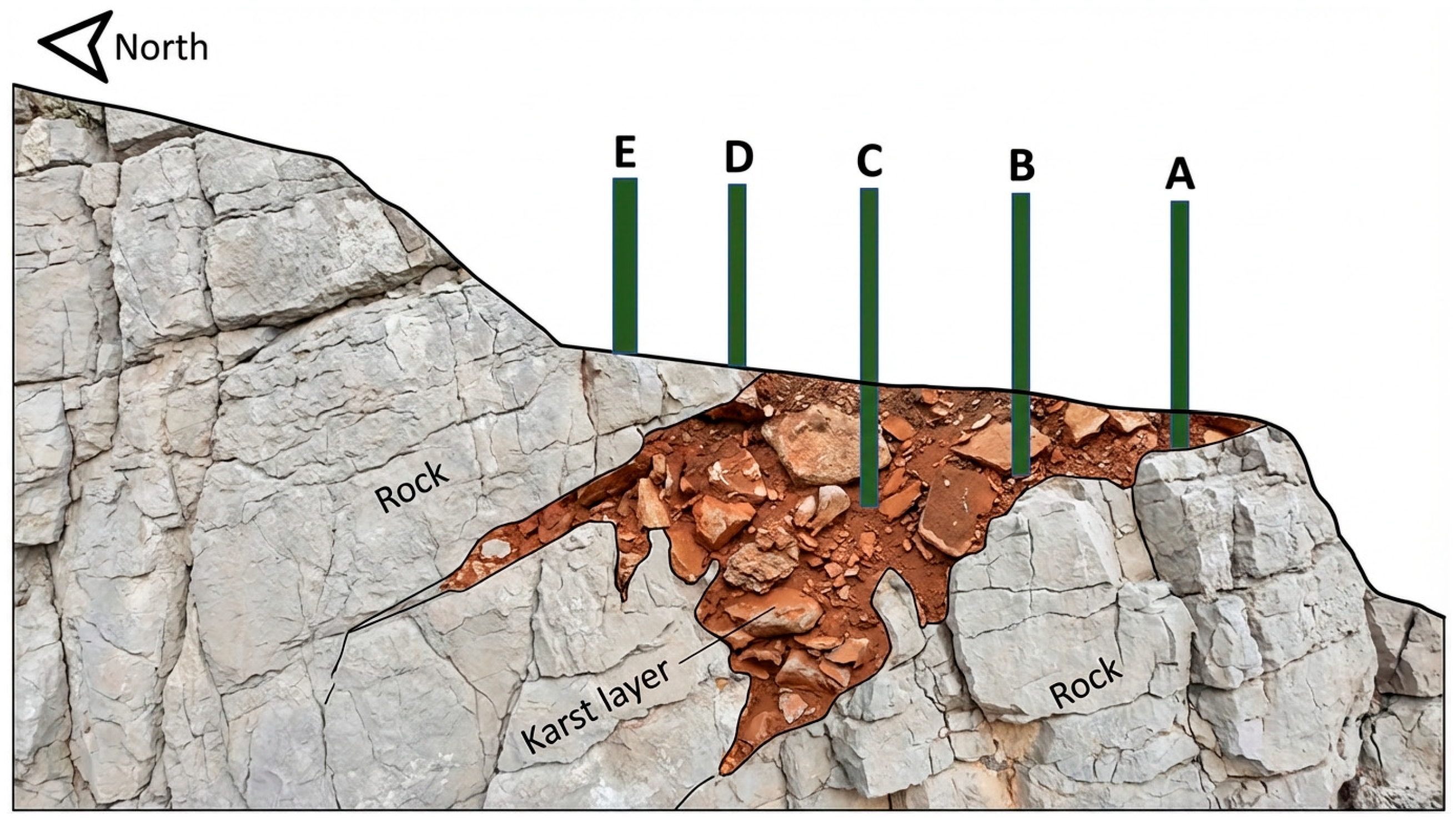
A schematic representation of the shallow subsoil was created (Figure 4) using data obtained from both geophysical methods. It is noteworthy that a karst layer is present entirely beneath row C. In contrast, row D is situated on its edge. Row E is placed directly on the bedrock (Figure 4). The filler layer beneath rows A and B is underlain by bedrock, with row A situated on the edge of the step (Figure 4). The results reveal a filler layer located beneath rows A, B, and C, with row D situated on its narrow edge and row E resting on the bedrock.

4. Discussion

This study investigated how subsurface geological structure (SSGS) influences vine physiology, growth, and wine quality in a terraced Merlot vineyard. By integrating physiological monitoring with geophysical surveys (ERT and GPR), we revealed that invisible subsoil heterogeneity creates vastly different growing conditions that override uniform management practices.

Gas exchange measurements exposed clear, geology-driven divergence among vineyard rows (Table 3). Early in the season, gas exchange parameters were similar across all rows, typical of non-stressed Merlot vines [19]. By mid-July, row C maintained high assimilation rates while rows A, B, D, and E declined sharply, indicating that the irrigation rate (35% ET_c) was adequate over the karst/fill system but insufficient over shallow bedrock. Stomatal conductance patterns paralleled these trends, with near-complete closure in row E by late summer and sustained moderate conductance in row C.

Stem water potential measurements confirmed a clear stress gradient (Table 2): rows C and B were relatively in moderate stress (~−1.2 MPa), rows D and E experienced severe stress (~−1.5 MPa or below), and row A hovered near the −1.4 MPa threshold reported as optimal for Merlot quality [20]. Wine scores followed this physiological pattern, where row A produced the highest quality, while insufficiently stressed rows C and B produced lower-quality wines. These results indicate that the SSGS created distinct zones of water availability that directly influenced vine physiological responses. The extremely low stomatal conductance values observed in late season (as low as ~5 mmol m⁻² s⁻¹; Table 3) reflect near-complete stomatal closure under severe water stress conditions. Such low gs values are consistent with the limited irrigation regime and late-season drought stress typical of Mediterranean vineyards under deficit irrigation management.

Yield and berry metrics reflected this water availability/vine physiology gradient (Table 4). Row C combined high bunch numbers with large berries (124.3 g per 100 berries versus 76.5–92.3 g elsewhere), producing the highest yield within the normal commercial range for Merlot vines [45]. Row E exhibited extreme yield reduction driven by low bunch and berry numbers rather than compensatory enlargement, consistent with severe, growth-limiting stress. Notably, yields across all treatments were very low, even relative to other mountainous vineyards in the same region, a pattern attributable in part to the absence of mineral fertilization and the use of a single compost application only once every 3–4 years. These findings align with recent work showing that spatial variation in soil moisture can drive differential physiological responses even within small vineyard areas [46].

Wine chemistry revealed a clear pathway from geological structure through water availability to quality. Row C’s higher water status produced the lowest Brix, anthocyanins, and phenolics (Table 5), reflecting dilution effects [20]. Row A moderately stressed achieved optimal balance with high phenolics, good color density, and the highest sensory scores of 88.78 points (Table 7). Row E, under extreme stress, produced highly concentrated wine (highest phenolics and color) but ranked only fourth in sensory evaluation due to elevated volatile acidity, lower alcohol, and early harvest, demonstrating that quality depends on balance rather than concentration alone. It is important to note that wine chemistry and sensory analysis results are based on single vinifications per row (n = 1 wine per treatment). While the observed chemical and sensory patterns are consistent with the physiological and yield differences among rows, these wine quality findings should be interpreted as indicative trends rather than definitive conclusions. Future studies employing replicated vinifications would strengthen the statistical inference regarding wine quality responses to subsoil geological structure.

The primary mechanism involves SSGS control over root system development and water access. Row E, over consolidated limestone, likely has a shallow effective rooting depth with roots confined to thin surface layers, creating minimal water storage that is rapidly depleted between irrigations [47]. Row C, over a karst cavity with fill material, enjoys deeper exploitable rooting (80–100 cm versus <60 cm over bedrock) and access to bedrock fissures that can extend root exploration to 3–4 m depth [48]. The sustained higher stomatal conductance in row C during peak stress strongly suggests the karst cavity acts as a subsurface reservoir, intercepting irrigation and lateral flows, then slowly releasing moisture through capillary redistribution [49].

Hydraulic properties further influence water movement. The heterogeneous fill material likely has higher conductivity, favoring infiltration but also faster drainage, while intact bedrock beneath row E acts as a low-permeability barrier promoting runoff rather than root-zone storage. Although nutrient differences cannot be ruled out, karst soils often differ in pH and micronutrient availability [50]. Several observations point to water as the dominant driver: differences intensified with seasonal progression, stomatal patterns reflect hydraulic rather than nutrient limitation [51], and quality effects align with classic deficit irrigation responses.

ERT and GPR imaging identified low-resistivity features beneath row C and high-resistivity bedrock beneath row E that correspond closely with vine performance patterns. While our subsurface model is inferred rather than directly measured, convergence between independent geophysical methods and strong functional agreement between inferred structure and vine responses under identical management provide compelling validation. The seasonal evolution of resistivity signatures matched expected Mediterranean moisture dynamics.

Several important limitations warrant acknowledgment. We did not directly observe root systems, leaving distribution and fissure penetration as inferred mechanisms. The study represents one vineyard over one season with one cultivar–rootstock combination. The quantitative integration of geophysical and agronomic data was limited by scale mismatches, with geophysical signals integrated over cubic-meter volumes, while vine measurements were point-based, and the small number of rows with strong spatial autocorrelation.

Our findings are specific to Merlot grafted onto 140 Ruggeri rootstock, which is suitable for poor soils, has high drought tolerance and high vigor [52,53]. Therefore, it had the best traits to handle the plot’s condition and still presented evident signs of stress. Nonetheless, drought-tolerant cultivars might show attenuated stress over bedrock, while more vigorous rootstocks could reduce SSGS-induced variability [53]. This suggests that geophysical SSGS characterization could guide strategic cultivar–rootstock placement and zone-specific management.

Moving toward quantitative precision viticulture requires intensive ground-truthing with soil pits and root mapping, time-series monitoring to capture seasonal dynamics, and three-dimensional geophysical characterization. Such advances would transform geophysical surveys from exploratory tools into robust decision-support systems for complex terroir management.

5. Conclusions

By integrating subsurface geological characterization with comprehensive vine and wine analysis, we demonstrated how hidden geological features create differential growing conditions that override surface management practices. The strong correspondence among subsurface structure, vine water status, berry chemistry, and wine quality provides compelling evidence for SSGS control over terroir expression. This research offers a framework for using non-invasive geophysical techniques to understand and manage terroir-driven variability, enabling precision strategies for variable-rate irrigation, targeted rootstock selection, zone-specific harvesting that accounts for the geological reality beneath the vines, and optimizing both yield and quality across spatially variable Mediterranean terraced vineyards.

References

1. Novara, A.; Pisciotta, A.; Minacapilli, M.; Maltese, A.; Capodici, F.; Cerdà, A.; Gristina, L. The impact of soil erosion on soil fertility and vine vigor. A multidisciplinary approach based on field, laboratory and remote sensing approaches. Sci. Total Environ. 2018, 622–623, 474–480. [Google Scholar] [CrossRef]
2. Bahat, I.; Netzer, Y.; Grünzweig, J.M.; Alchanatis, V.; Peeters, A.; Goldshtein, E.; Ohana-Levi, N.; Ben-Gal, A.; Cohen, Y. In-Season Interactions between Vine Vigor, Water Status and Wine Quality in Terrain-Based Management-Zones in a ‘Cabernet Sauvignon’ Vineyard. Remote Sens. 2021, 13, 1636. [Google Scholar] [CrossRef]
3. Ohana-Levi, N.; Knipper, K.; Kustas, W.P.; Anderson, M.C.; Netzer, Y.; Gao, F.; Alsina, M.d.M.; Sanchez, L.A.; Karnieli, A. Using Satellite Thermal-Based Evapotranspiration Time Series for Defining Management Zones and Spatial Association to Local Attributes in a Vineyard. Remote Sens. 2020, 12, 2436. [Google Scholar] [CrossRef]
4. Morlat, R.; Bodin, F. Characterization of Viticultural Terroirs using a Simple Field Model Based on Soil Depth—II. Validation of the Grape Yield and Berry Quality in the Anjou Vineyard (France). Plant Soil 2006, 281, 55–69. [Google Scholar] [CrossRef]
5. Passioura, J.B. Soil structure and plant growth. Aust. J. Soil Res. 1991, 29, 717–728. [Google Scholar] [CrossRef]
6. Sung, C.T.B.; Ishak, C.F.; Abdullah, R.; Othman, R.; Panhwar, Q.A.; Aziz, M.M.A. Soil properties (physical, chemical, 567 biological, mechanical). In Soils of Malaysia; CRC Press: Boca Raton, FL, USA, 2017; pp. 103–154. [Google Scholar]
7. De Neve, S.; Pannier, J.; Hofman, G. Temperature effects on C- and N-mineralization from vegetable crop residues. Plant Soil 1996, 181, 25–30. [Google Scholar] [CrossRef]
8. Radford, B.J.; Yule, D.F.; McGarry, D.; Playford, C. Crop responses to applied soil compaction and to compaction repair treatments. Soil Tillage Res. 2001, 61, 157–166. [Google Scholar] [CrossRef]
9. Ferree, D.C.; Streeter, J.G. Response of container-grown grapevines to soil compaction. HortScience 2004, 39, 1250–1254. [Google Scholar] [CrossRef]
10. Nawaz, M.F.; Bourrié, G.; Trolard, F. Soil compaction impact and modelling. A review. Agron. Sustain. Dev. 2013, 33, 291–309. [Google Scholar] [CrossRef]
11. Tramontini, S.; van Leeuwen, C.; Domec, J.-C.; Destrac-Irvine, A.; Basteau, C.; Vitali, M.; Mosbach-Schulz, O.; Lovisolo, C. Impact of soil texture and water availability on the hydraulic control of plant and grape-berry development. Plant Soil 2013, 368, 215–230. [Google Scholar] [CrossRef]
12. Batey, T.; McKenzie, D.C. Soil compaction: Identification directly in the field. Soil Use Manag. Ment. 2006, 22, 123–131. [Google Scholar] [CrossRef]
13. Lakso, A.N.; Pool, R. Drought stress effects on vine growth, function, ripening and implications for wine quality. In Proceedings of the 29th Annual New York Wine Industry Workshop, Geneva, NY, USA, 2000; Cornell University: Ithaca, NY, USA, 2000; pp. 86–90. [Google Scholar]
14. Ohana-Levi, N.; Munitz, S.; Netzer, Y. Grapevine stem water potential seasonal curves: Response to meteorological conditions, and association to yield and red wine quality. Agric. For. Meteorol. 2023, 342, 109755. [Google Scholar] [CrossRef]
15. Zhang, Y.; Zhao, J.; Xu, J.; Chai, Y.; Liu, P.; Quan, J.; Wu, X.; Li, C.; Yue, M. Effects of Water Availability on the Rela-tionships Between Hydraulic and Economic Traits in the Quercus wutaishanica Forests. Front. Plant Sci. 2022, 13, 902509. [Google Scholar] [CrossRef]
16. Arias, L.A.; Berli, F.; Fontana, A.; Bottini, R.; Piccoli, P. Climate Change Effects on Grapevine Physiology and Biochemistry: Benefits and Challenges of High Altitude as an Adaptation Strategy. Front. Plant Sci. 2022, 13, 835425. [Google Scholar] [CrossRef]
17. Matese, A.; Baraldi, R.; Berton, A.; Cesaraccio, C.; Di Gennaro, S.F.; Duce, P.; Facini, O.; Mameli, M.G.; Piga, A.; Zaldei, A. Estimation of Water Stress in Grapevines Using Proximal and Remote Sensing Methods. Remote Sens. 2018, 10, 114. [Google Scholar] [CrossRef]
18. Chacón-Vozmediano, J.L.; Martínez-Gascueña, J.; García-Navarro, F.J.; Jiménez-Ballesta, R. Effects of water stress on vegetative growth and ‘Merlot’ grapevine yield in a semi-arid Mediterranean climate. Horticulturae 2020, 6, 95. [Google Scholar] [CrossRef]
19. Munitz, S.; Netzer, Y.; Schwartz, A. Sustained and regulated deficit irrigation of field-grown Merlot grapevines. Aust. J. Grape Wine Res. 2017, 23, 87–94. [Google Scholar] [CrossRef]
20. Peterlunger, E.; Sivilotti, P.; Colussi, V. Water stress increased polyphenolic quality in ‘Merlot’ grapes. In Proceedings of the VII International Symposium on Grapevine Physiology and Biotechnology 689, Davis, CA, USA, 21–25 June 2004; pp. 293–300. [Google Scholar] [CrossRef]
21. Fanourakis, D.; Aliniaeifard, S.; Sellin, A.; Giday, H.; Körner, O.; Rezaei Nejad, A.; Delis, C.; Bouranis, D.; Koubouris, G.; Kambourakis, E.; et al. Stomatal behavior following mid- or long-term exposure to high relative air humidity: A review. Plant Physiol. Biochem. 2020, 153, 92–105. [Google Scholar] [CrossRef]
22. Mulla, D.J.; McBratney, A.B. Soil spatial variability. In Soil Physics Companion; CRC Press: Boca Raton, FL, USA, 2001; pp. 343–373. [Google Scholar]
23. Mirás-Avalos, J.M.; Fandiño, M.; Rey, B.J.; Dafonte, J.; Cancela, J.J. Zoning of a Newly-Planted Vineyard: Spatial Variability of Physico-Chemical Soil Properties. Soil Syst. 2020, 4, 62. [Google Scholar] [CrossRef]
24. Doolittle, J.A.; Collins, M.E. Use of soil information to determine application of ground penetrating radar. J. Appl. Geophys. 1995, 33, 101–108. [Google Scholar] [CrossRef]
25. André, F.; van Leeuwen, C.; Saussez, S.; Van Durmen, R.; Bogaert, P.; Moghadas, D.; de Rességuier, L.; Delvaux, B.; Vereecken, H.; Lambot, S. High-resolution imaging of a vineyard in south of France using ground-penetrating radar, electromagnetic induction and electrical resistivity tomography. J. Appl. Geophys. 2012, 78, 113–122. [Google Scholar] [CrossRef]
26. Mary, B.; Peruzzo, L.; Boaga, J.; Cenni, N.; Schmutz, M.; Wu, Y.; Hubbard, S.S.; Cassiani, G. Time-lapse monitoring of root water uptake using electrical resistivity tomography and mise-à-la-masse: A vineyard infiltration experiment. Soil 2020, 6, 95–114. [Google Scholar] [CrossRef]
27. Martini, E.; Comina, C.; Priori, S.; Costantini, E.A.C. A combined geophysical-pedological approach for precision viticulture in the Chianti hills. Boll. Geofis. Teor. Appl. 2013, 54, 165–181. [Google Scholar] [CrossRef]
28. Netzer, Y.; Munitz, S.; Shtein, I.; Schwartz, A. Structural memory in grapevines: Early season water availability affects late season drought stress severity. Eur. J. Agron. 2019, 105, 96–103. [Google Scholar] [CrossRef]
29. Sneh, A.; Bartov, Y.; Weissbrod, T.; Rosensaft, M. Geological Map of Israel 1:200,000; Israel Geological Survey: Jerusalem, Israel, 1998.
30. Hurlbert, S.H. Pseudoreplication and the design of ecological field experiments. Ecol. Monogr. 1984, 54, 187–211. [Google Scholar] [CrossRef]
31. Van Leeuwen, C.; Roby, J.-P.; de Rességuier, L. Soil-related terroir factors: A review. OENO One 2018, 52, 173–188. [Google Scholar] [CrossRef]
32. Van Leeuwen, C.; Destrac-Irvine, A.; Dubernet, M.; Duchêne, E.; Gowdy, M.; Marguerit, E.; Pieri, P.; Parker, A.; de Rességuier, L.; Ollat, N. An Update on the Impact of Climate Change in Viticulture and Potential Adaptations. Agronomy 2019, 9, 514. [Google Scholar] [CrossRef]
33. Kennedy, J.A. Understanding Grape Berry Development; Practical Winery & Vineyard: San Rafael, CA, USA, 2002; pp. 1–5. [Google Scholar]
34. Boyer, J.S.; Westgate, M.E. Grain yields with limited water. J. Exp. Bot. 2004, 55, 2385–2394. [Google Scholar] [CrossRef] [PubMed]
35. Loke, M.H. Tutorial: 2-D and 3-D Electrical Imaging Surveys; Geotomo Software: Gelugor, Malaysia, 2004. [Google Scholar]
36. Smart, R.E.; Robinson, M.D. Sunlight into Wine: A Handbook for Winegrape Canopy Management; Winetitles: Adelaide, Australia, 1991. [Google Scholar]
37. Huisman, J.A.; Hubbard, S.S.; Redman, J.D.; Annan, A.P. Measuring soil water content with ground penetrating radar: A review. Vadose Zone J. 2003, 2, 476–491. [Google Scholar] [CrossRef][Green Version]
38. Telford, W.M.; Geldart, L.P.; Sheriff, R.E. Applied Geophysics, 2nd ed.; Cambridge University Press: Cambridge, UK, 1990. [Google Scholar] [CrossRef]
39. Samouëlian, A.; Cousin, I.; Tabbagh, A.; Bruand, A.; Richard, G. Electrical resistivity survey in soil science: A review. Soil Tillage Res. 2005, 83, 173–193. [Google Scholar] [CrossRef]
40. Chalikakis, K.; Plagnes, V.; Guerin, R.; Valois, R.; Bosch, F.P. Contribution of geophysical methods to karst-system exploration: An overview. Hydrogeol. J. 2011, 19, 1169–1180. [Google Scholar] [CrossRef]
41. OIV (International Organisation of Vine and Wine). OIV Compendium of International Methods of Wine and Must Analysis; Edition 2021; OIV: Paris, France, 2021. [Google Scholar]
42. Loke, M.H.; Chambers, J.E.; Rucker, D.F.; Kuras, O.; Wilkinson, P.B. Recent developments in the direct-current geoelectrical imaging method. J. Appl. Geophys. 2013, 95, 135–156. [Google Scholar] [CrossRef]
43. Daniels, D.J. Ground Penetrating Radar, 2nd ed.; The Institution of Engineering and Technology: London, UK, 2004. [Google Scholar] [CrossRef]
44. Archie, G.E. The electrical resistivity log as an aid in determining some reservoir characteristics. Trans-Actions AIME 1942, 146, 54–62. [Google Scholar] [CrossRef]
45. Friedman, S.P. Soil properties influencing apparent electrical conductivity: A review. Comput. Electron. Agric. 2005, 46, 45–70. [Google Scholar] [CrossRef]
46. Yu, R.; Brillante, L.; Martínez-Lüscher, J.; Kurtural, S.K. Spatial variability of soil and plant water status and their cascading effects on grapevine physiology are linked to berry and wine chemistry. Front. Plant Sci. 2020, 11, 790. [Google Scholar] [CrossRef] [PubMed]
47. Shellie, K.C. Water productivity, yield and berry composition in sustained versus regulated deficit irrigation of Merlot grapevines. Am. J. Enol. Vitic. 2014, 65, 197–205. [Google Scholar] [CrossRef]
48. Comas, L.H.; Anderson, L.J.; Dunst, R.M.; Lakso, A.N.; Eissenstat, D.M. Canopy and environmental control of root dynamics in a long-term study of Concord grape. New Phytol. 2005, 167, 829–840. [Google Scholar] [CrossRef] [PubMed]
49. Archer, E.; Strauss, H. Effect of Shading on the Performance of Vitis Vinif Era L. Cv. Cabernet Sauvignon. S. Afr. J. Enol. Vitic. 2017, 10, 74–76. [Google Scholar] [CrossRef]
50. Caldwell, M.M.; Dawson, T.E.; Richards, J.H. Hydraulic lift: Consequences of water efflux from the roots of plants. Oecologia 1998, 113, 151–161. [Google Scholar] [CrossRef]
51. Seguin, G. ‘Terroirs’ and pedology of wine growing. Experientia 1986, 42, 861–873. [Google Scholar] [CrossRef]
52. Chaves, M.M.; Zarrouk, O.; Francisco, R.; Costa, J.M.; Santos, T.; Regalado, A.P.; Rodrigues, M.L.; Lopes, C.M. Grapevine under deficit irrigation: Hints from physiological and molecular data. Ann. Bot. 2010, 105, 661–676. [Google Scholar] [CrossRef] [PubMed]
53. Marguerit, E.; Brendel, O.; Lebon, E.; Van Leeuwen, C.; Ollat, N. Rootstock control of scion transpiration and its acclimation to water deficit are controlled by different genes. New Phytol. 2012, 194, 416–429. [Google Scholar] [CrossRef] [PubMed]
Figure 1. Compares inverted ERT3 profiles in the winter (upper) and summer (lower). The top graph was measured during winter, while the bottom graph was measured during summer, cv. Merlot, Dolev vineyard, 2021. The y-axis is elevation relative to ground level (m), and the x-axis is the distance from the measurement starting point (m).
Agriculture 16 00630 g001
Figure 2. Comparison of GPR measurements in row C in winter (top) and summer (bottom). The y-axis is time (ns), and the x-axis is the distance from the measurement starting point (m). The top graph was measured during winter, while the bottom was measured during summer, cv. Merlot, Dolev vineyard, 2021.
Agriculture 16 00630 g002
Figure 3. Wintertime comparison between row C (line ERT3 and GPR5) and row E (ERT1 and GPR1) of both the ERT and GPR methods. The top graph shows the elevation relative to ground level (m) on the y-axis and the distance from the measurement starting point (m) on the x-axis. In the bottom graph, the y-axis represents time (ms), and the x-axis represents the distance from the starting point (m) for all graphs. cv. Merlot, Dolev vineyard, 2021.
Agriculture 16 00630 g003
Figure 4. Cross-section schematic of the Merlot grapevine plot in Dolev based on geophysical data collected in this work. Vine rows are marked from A to E.
Agriculture 16 00630 g004