Formulation of Nutrient Solutions Using Simulated Annealing

Guerra Ibarra, Juan Pablo; Cuevas de la Rosa, Francisco Javier; Rocha Rocha, Aaron Junior

doi:10.3390/agriculture16040449

Open AccessArticle

Formulation of Nutrient Solutions Using Simulated Annealing

by

Juan Pablo Guerra Ibarra

^1,*

,

Francisco Javier Cuevas de la Rosa

²

and

Aaron Junior Rocha Rocha

¹

Instituto Tecnológico Nacional de México, Campus Zamora, Computer Systems Engineering Academy, Zamora 59720, Michoacán, Mexico

²

Centro de Investigaciones en Óptica A.C., León 37150, Guanajuato, Mexico

^*

Author to whom correspondence should be addressed.

Agriculture 2026, 16(4), 449; https://doi.org/10.3390/agriculture16040449

Submission received: 30 December 2025 / Revised: 22 January 2026 / Accepted: 28 January 2026 / Published: 14 February 2026

(This article belongs to the Section Artificial Intelligence and Digital Agriculture)

Download

Browse Figures

Versions Notes

Abstract

Modern agriculture requires optimizing available resources to maximize production while minimizing environmental impact without increasing economic costs. Hydroponic agriculture replaces soil with inert media that provide physical support for plants but do not supply nutrients. In this type of agricultural production, fertilization with nutrient solutions is essential, as they supply the 15 elements necessary for proper plant development. These solutions consist of mixtures of different amounts of fertilizers dissolved in water. In this context, a method based on a simulated annealing algorithm is proposed, a metaheuristic that optimizes fertilizer quantities in grams to achieve target concentrations in parts per million for six macronutrients and nine micronutrients. The algorithm addresses a multi-objective optimization problem, balancing two competing goals: first, maximizing the accuracy of the fertilizer balance to achieve the required nutritional levels, and second, minimizing the total cost of the fertilizer mixture. The algorithm’s fitness function weights the total cost of the fertilizers used and the total relative error between the concentrations obtained and those desired, allowing the relative importance of cost and accuracy in the nutrient solution to be adjusted. The results of three experiments with varying nutrient levels are presented for a 1000-L water tank. The first experiment consisted of three macronutrients and two micronutrients. The second configuration added three macronutrients and two micronutrients, for a total of ten nutrients. Finally, five micronutrients were added to complete the 15 essential nutrients for plants. It is important to note that there are several methods for calculating micronutrients that contribute to precision agriculture, increasing the complexity of finding a solution that meets established nutritional requirements. The nutrient concentrations in parts per million required for tomato cultivation during the vegetative development stage. To balance nutrient accuracy and solution cost, we applied weighting factors of

0.65, 0.75, 0.85, 0.90, 0.95,

and

1.0

for accuracy. The corresponding weights for cost were calculated as the complement of these values (totaling 1). By favoring nutrient accuracy with a weighting of 1, accuracies of 0.00500, 0.02618, and 0.03077 parts per million were achieved in each experiment, respectively. Meanwhile, the lowest cost is

2.06

,

2.72

, and

2.70

USD for the aforementioned experiments.

Keywords:

hydroponics; metaheuristics; nutrient solution; precision agriculture; simulated annealing

1. Introduction

Agriculture is a pillar of human sustenance and the development of civilizations around the world [1,2]. It supports population growth by producing sufficient food in terms of quantity and quality, ideally without increasing costs or environmental impact. By 2050, the United Nations [3] forecasts a world population of approximately 10 billion, which poses challenges in a context of declining arable land, which currently represents

45 %

of the Earth’s surface [4] but produces increasingly more food, making it necessary to seek sustainable alternatives, such as hydroponics, instead of extensive practices.

Recent technological advances in tillage have given rise to Precision Agriculture (PA), which uses statistics and different types of algorithms, ranging from classic to Artificial Intelligence (AI), such as Computer Vision (CV) [1], Deep Learning (DL), and Metaheuristics (MA) [5,6]. PA aims to increase crop yields and resource efficiency by monitoring crop characteristics such as growth, leaf and fruit color, and health, while optimizing irrigation and fertilization to reduce environmental impact and detect pests and diseases [7,8,9].

Simulated Annealing Algorithm (SA) is inspired by a metallurgical process. Annealing constitutes a heat treatment process in metallurgy wherein a metal is heated to an elevated temperature to enhance atomic mobility, followed by controlled cooling to attain a minimum-energy crystalline structure, thereby improving ductility and relieving internal stresses. The SA represents a trajectory-based stochastic metaheuristic tailored for global optimization in search spaces exhibiting complex topologies with multiple local optima [10].

This document develops and presents an adapted SA method for formulating hydroponic nutrient solutions, highlighting key aspects: applicability across diverse hydroponic crops, effectiveness in meeting crop specific nutritional requirements, substantial fertilizer cost reductions via a weighting parameter balancing both factors without compromising nutrient adequacy and most methods in the literature focus on the three main macronutrients, while the method presented here covers the elements that are essential for plant development.

The organization of the paper is as follows: Section 2 presents a series of works related to land cultivation processes for food production in PA. Section 3 The materials and methods used in the SA adaptation for the formulation of nutrient solutions for crops are described. The objectives of the experiment and the control parameters for the formulation of nutrient solutions using SA are presented in Section 4. The results obtained with the adaptation of the algorithm for the formulation of nutrient solutions are presented in the Section 5 and the Section 6 contains the conclusions of the research.

2. Related Works

The technification of agricultural processes with the aim of achieving the objectives of the PA has led to the use of different types of hardware and software, which are constantly updated to improve their efficiency. The use of intelligent algorithms has recently been used in several tasks such as identification of pests, diseases [11,12], classification of plant components in crops [13,14,15], and optimization of irrigation and fertilization processes [16,17].

Various methods have been reported in the literature for PA to determine the levels of certain chemical elements in crops, with a focus on nitrogen, phosphorus, and potassium. Lu [18] used 340 groups of images with different potassium contents to establish the relationship between reflectance spectra and leaf K content. Qi [19] proposed a method for determining the nitrogen content in images of wheat crops acquired with mobile devices using histogram manipulation algorithms. Phosphorus is another of the main macronutrients for crop development. Li [20] presented a method for measuring how phosphorus concentration affects electrical impedance in tomato crops. Sun [21] used dynamic leaf capture of rice leaves by scanning to investigate the changing regulation of leaf characteristics under nutritional stress from nitrogen, phosphorus, and potassium. Leaf characteristics were determined using the mean value and regionprops functions, and leaf dynamics were quantified by calculating the relative growth rate. Tran [22] implemented the Inception-ResNet v2 convolutional neural network model and Autoencoder to classify and predict calcium, potassium, and nitrogen deficiencies.

Once a nutrient deficiency has been identified, the next step in PA is to correct the condition through fertilization processes that must be both effective and efficient. For example, Cropper [17] developed a model to estimate the amount of phosphorus present in the soil and crop requirements in order to use a genetic algorithm to estimate the minimum amount needed to meet crop needs through fertilization processes. Xu [23] developed an expert system to support decision-making regarding nitrogen, phosphorus, and potassium fertilization processes, using data from 2000 plant nutrition experiments, reporting an increase in rice grain production in fields that used the recommendations made by the expert system. Ahmad [24] estimated the amount of nitrogen needed based on the water required for its application using a quadratic equation that can be used to reduce costs across different crops. Ahmed [25] implemented a genetic algorithm that uses data from different types of sensors to make adjustments to fertilization processes, using the neighborhood-based strategy for the exploration and exploitation stages. Chen [26] proposed an optimization method based on an optimization algorithm inspired by the behavior of the gray wolf with multiple strategies to make fertilization suggestions for the main macronutrients.

3. Materials and Methods

The following sections describe the fundamental concepts of the formulation of nutritional solutions, characteristics of the crop selected for experimentation, and the explanation of the method for Formulating Nutrient Solutions Using Simulated Annealing (FNSUSA).

3.1. Plant Nutrition

Through photosynthesis, plants obtain essential elements such as Oxygen (O), Carbon (C), and Hydrogen (H). Additionally, proper plant development requires 15 other essential chemical elements, which are divided into two categories: six macronutrients [27] and nine micronutrients [28]. This division is based on the quantity required, not on their relative importance. The elements belonging to the first category are required in greater quantities compared to elements belonging to the second category; for macronutrients, the range is from 30 to 400 PPM and for micronutrients, it is 0.01–5 PPM [29], emphasizing that each crop has specific needs. Table 1 shows the chemical elements belonging to each category.

Soilless cultivation of various crops, primarily vegetables, in greenhouses requires a consistent, efficient, and effective fertilization process [30]. This approach enhances both the quantity and quality of harvests, enables off-season production, and opens opportunities for accessing export markets, among other benefits. To provide crops with essential resources for growth that are not acquired through photosynthesis, different amounts of fertilizers are mixed or dissolved in 1000 L of water in one-cubic-meter tanks, which are commonly used in hydroponics. The mixture is called the Nutrient Solution (NS). Table 2 shows the chemical composition of some fertilizers commonly used in the composition of NS. Fertilizer prices were taken directly from online shopping sites such as eBay (https://mx.ebay.com accessed on 4 November 2025), Amazon (https://www.amazon.com.mx accessed on 14 November 2025), and MercadoLibre (https://www.mercadolibre.com.mx accessed on 10 December 2025).

The total cost of an NS is calculated by adding the price of each fertilizer used in the mixture by the amount in grams used, which is expressed in the following equation:

C o s t_{N S} = \sum_{f = 0}^{n} (\frac{q_{f}}{1000}) \times P_{f},

(1)

where n is the number of fertilizers available to formulate the NS;

q_{f}

is the amount of each fertilizer expressed in grams for mixing;

P_{f}

refers to the cost by kg of fertilizer f on the market.

To formulate NS, it is necessary to calculate the Parts Per Million (PPM) of each Nutrient chemical element present in a given amount in grams of fertilizer. The PPM of a specific element is calculated using the following equation:

P P M_{e}^{f} = \frac{1000 \times q_{f} \times a_{e} \times n_{e}^{f}}{m w^{f} \times V},

(2)

where f refers to a particular fertilizer, and e is the nutrient that forms part of the fertilizer, 1000 is constant conversion factor to convert grams of fertilizer to milligrams,

q_{f}

is the amount in grams of fertilizer,

a_{e}

is the atomic weight of the element selected for its quantification,

n_{e}^{f}

is the number of atoms of the chemical element present in chemical formula of one fertilizer particularly,

a w^{f}

is the fertilizer molecular weight and V is total volume of the NS in liters.

NS is a mixture of various quantities of fertilizers, each of which contributes a different PPM of the nutrient elements. Therefore, it is necessary to quantify the total PPM of each chemical element present in the NS. The following equation is used to determine the PPM of the different Nutrient elements:

P P M_{e}^{N S} = \sum_{f = 0}^{n} P P M_{e}^{f},

(3)

where

P P M_{e}^{N S}

represents the total concentration of the nutrient element e present in the NS, while

P P M_{e}^{f}

corresponds to the amount of PPM contributed by a specific amount of fertilizer f for nutrient element e, calculated by applying Equation (2).

3.2. Algorithm for Formulating Nutritious Solutions Using Simulated Annealing

Simulated Annealing (SA) is a metaheuristic algorithm inspired by the metallurgical process of annealing, in which a material is slowly cooled to reach a minimum-energy state. Its primary strength lies in its ability to escape local optima, making it ideal for complex combinatorial optimization problems with vast search spaces, such as the

N S

Formulation. The algorithm operates by iteratively exploring solutions, starting at a high initial “temperature”. In each step, a neighboring solution is generated; better solutions are always accepted, while worse solutions may also be accepted based on a probabilistic criterion tied to the current temperature. Initially, this allows the algorithm to broadly explore the solution space (exploration phase). As the process continues, the temperature is gradually reduced according to a cooling schedule, which decreases the probability of accepting worse solutions. This shifts the search from exploration to exploitation, allowing the algorithm to converge towards a globally optimal solution. The main control parameters are the initial and final temperatures, the cooling factor, and the number of iterations at each temperature level [31].

It is necessary to initially assign a quantity, in grams, of each available fertilizer for the formulation of the NS. This is done by applying the Equation:

q_{f} = r a n d o m (l l, u l),

(4)

where the quantity in grams for fertilizer f is between the lower limit (

l l

) and the upper limit (

u l

), which are used for all fertilizers available for the formulation of NS.

The algorithm begins by creating a random initial candidate solution in the search space, which is as follows:

S_{a} = {q_{1}, q_{2}, \dots, q_{f - 1}, q_{f}},

(5)

where n is the number of fertilizers available for the formulation of NS.

The SA explores the search space by introducing a perturbation in the

S_{a}

. The perturbations for each

q_{f} \in S_{a}

are determined based on the following equation:

ρ_{f} = r a n d o m (0, E_{v}),

(6)

where

E_{v}

represents the upper limit of the perturbation to explore the search space, which is in the range

[0, 1]

. This value decreases linearly with the system temperature, allowing the exploitation stage to be emphasized.

The increase or decrease for

q_{n} \in S_{a}

is determined by the following equation:

r_{f} = q_{f} * ρ_{f} .

(7)

SA requires a second solution to the problem to be optimized, which is constructed from

S_{a}

applying the following equation:

S_{c} = {q_{1} \pm r_{1}, q_{2} \pm r_{2}, \dots, q_{f - 1} \pm r_{f - 1}, q_{f} \pm r_{f}} .

(8)

where

S_{c}

is the candidate solution constructed from

S_{a}

. The quantities of each fertilizer

q_{f}

are increased or decreased randomly, with the same probability of occurrence.

It is important to note that

q_{n}

cannot be negative. If a negative value is generated for any

q_{n}

, it will take the value of 0.

FNSUSA is a random optimization algorithm whose main feature is that, at the beginning of execution, it favors exploration of the search space, allowing it to accept solutions that are not necessarily better than the current one. As the current solution’s fitness approaches the convergence condition, the exploitation stage of the search space is emphasized.

The objective of FNSUSA is to identify a fertilizer formulation that achieves the target concentrations in PPM for the macronutrients and micronutrients specified in Table 2. The target PPM is defined by the following equation:

P P M_{e} = {P P M_{1}, P P M_{2}, \dots, P P M_{e - 1}, P P M_{e}},

(9)

where subscript e refers to the nutrient element established as the target to be achieved in the final NS in PPM.

Relative error is an option for measuring the accuracy of the NS PPMs in relation to the target PPMs. It is expressed using the following equation:

R E_{e} = \frac{∣ P P M_{e} - P P M_{e}^{N S} ∣}{P P M_{e}},

(10)

where

R E_{e}

is the absolute relative error of nutrient e, in relation to the

P P M_{e}^{N S}

defined in Equation (3) with respect to

P P M_{e}^{t}

.

The total relative error in the NS is determined by applying the Equation:

R E_{t o t a l} = \sum_{e = 1}^{O} R E_{e} .

(11)

Subindex e takes values from 1 to the total number of nutrients

(O)

considered in the objective function of the FNSUSA.

The success of metaheuristic algorithms, including SA, largely depends on how the cost or fitness function is modeled. In the case of FNSUSA, the fitness function is a linear weighted sum combining two metrics:

R E_{t o t a l}

and

C o s t_{N S}

. This is expressed in the following equation:

A p t i t u d e_{N S} = (γ * R E_{t o t a l}) + ((1 - γ) * C o s t_{N S}),

(12)

where

γ

is the preponderance factor between the total relative error and the cost of NS, it must take a value in the range

[0, 1]

; similarly, this value acts as a normalizer between the two parameters to be weighted. It is important to mention that as the total relative error tends to 0, the cost of NS will naturally take on greater importance in determining the fitness of an NS.

The initial temperature and the model for its reduction (the cooling schedule) are key parameters for controlling the algorithm’s exploration phase. The initial temperature [32] of the FNSUSA is calculated using the following equation:

t = \frac{Δ}{- l n (p)},

(13)

where

Δ

is the difference between the fitness of the initial solution and the candidate solution, and p is the desired probability of accepting worse solutions at the start of the FNSUSA.

The temperature parameter is reduced geometrically, applying the following equation:

t = t * α,

(14)

where

α

is an initial value that must be in the range [0, 1]; a value close to 1 generates a slight decrease in temperature, while a value tending to 0 causes accelerated cooling. The decrement factor

α

is calculated using Equation:

α = {(\frac{t_{f}}{t})}^{1 / I},

(15)

where

t_{f}

is the desired final temperature of the system or convergence condition, and I is the number of energy states through which the system passes.

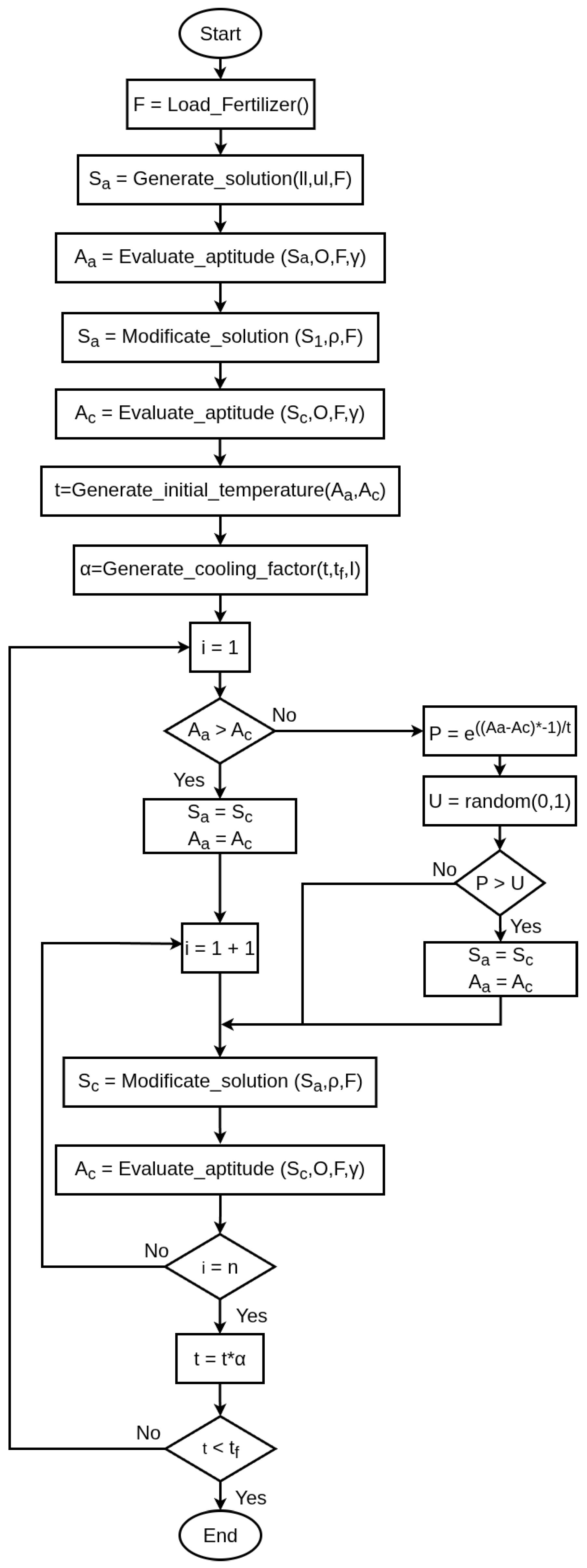
Figure 1 illustrates the adaptation of the SA algorithm for formulating hydroponic Nutrient Solutions.

The diagram outlines the primary functions responsible for implementing the previously described equations. A general description of each function, its parameters, and its return values is provided in Table 3.

3.3. Development Environment and Computer Specifications

The programming language in which the algorithm in Figure 1 was implemented was Python version 3.9.15, due to the number of libraries available. The hardware characteristics are necessary to provide a reference for the time required for the FNSUSA algorithm to reach the target PPM.

The characteristics of the computer equipment that was used were as follows:

Manufacturer: ASUSTeK COMPUTER INC., Taipei City, China
Modelo: X510UNR
Processor: Intel^® Core™ i7-8550U CPU @ 1.80 GHz × 8.
RAM: 16 GB.
Operating system: Ubuntu 22.04.2 LTS 64 bits.

4. Experimentation

The efficiency of the FNSUSA algorithm is measured in two ways. The first scenario evaluates the algorithm’s effectiveness in achieving the target PPMs (for macronutrients or micronutrients). This is achieved by assigning

γ = 1

, a parameterization that (based on Equation (12)) nullifies the cost component, forcing the optimization to focus exclusively on technical effectiveness. The second scenario tests the method’s ability to balance achieving the PPM against a lower price. For this test, the cost is explicitly considered by assigning

γ

a value between zero and one

(0 \leq γ \leq 1)

. A total of 180 FNSUSA executions are reported, 10 for each of the six

γ

values tested, giving a total of 60 executions and 3 different target configurations, for a total of 180.

4.1. Characteristics of Selected Crop for the Step of Experimentation

Our experimental stage focuses on the tomato, a member of the Solanaceae family with its origins in the Americas. There are two hypothesized beginnings for its domestication: one in the mountainous areas of Peru and Ecuador, and the other in the Aztec Empire’s Tenochtitlan [33]. The tomato crop has several developmental stages during its growth, which differ in terms of water and nutrient requirements versus the development of the plant itself. The developmental stages are as follows:

Plant establishment: Tomato is a crop that can be annual or perennial. It germinates four to seven days after the seed is sown. The root begins to develop, and the formation of the aerial part of the plant begins.
Vegetative growth: In this period, the plant grows rapidly, flowering and developing fruit. After 70 days, vegetative development is minimal, as well as the accumulation of dry matter in leaves and stems. Development.
Flowering and fruit set: Flowering and fruit set begin about 20–40 days after transplanting and continue during the rest of the growth cycle.
Fruit development: The fruit begins to develop and grow, accumulating in this period the greatest amount of dry matter in the fruit at a relatively stable rate.
Physiological maturity and harvest: Fruit maturity is achieved between 80 and 120 days after transplanting. Harvesting is permanent.

4.2. Results of FNSUSA

Three different nutritional objectives are presented as targets for the FNSUSA. These objectives are defined by the number of macronutrients and micronutrients to be balanced, starting at five and increasing to 15 essential nutrients, for tomato cultivation during its vegetative growth stage [34,35]. The combination of macronutrients and micronutrients for each fitness function is shown in Table 4.

As illustrated in Figure 1, FNSUSA requires several key parameters to guide its execution. These parameters are essential for formulating an NS that satisfies the objectives defined by the fitness function. The specific values configured for this implementation are as follows:

Initial temperature calculated using the Equation (13).
Final temperature $t_{f} = 1$ .
The value of $α$ is determined using Equation (15).
Low limit $l l = 10$ .
Upper limit $u l = 500$ .
$E_{v} = 0.15$ .

This specific parameter set was established to ensure the algorithm properly explores the solution space while balancing search breadth with an efficient convergence speed.

5. Results

The results presented apply FNSUSA to balance the relationship between the

R E_{t o t a l}

, measured as the relative error between the target PPMs and those contained in the NS, and the cost of NS, using different values assigned to

γ

. The first configuration has five nutrients, three macronutrients and two micronutrients; the second configuration adds the remaining three macronutrients and two micronutrients, for a total of ten target PPMs; the final arrangement adds the remaining five micronutrients for a total of 15 PPM targets to achieve.

Ten FNSUSA runs are performed for each of the three experimental configurations of target PPM presented in Table 4. To evaluate the algorithm’s efficiency in balancing total error (

R e_{t o t a l}

) and cost within the NS formulation, the weighting parameter

γ

was tested at values of

0.65, 0.75, 0.85, 0.90, 0.95,

and

1.0

. This approach allows for a precise calibration of the trade-off between accuracy and nutrient solution costs.

5.1. Results Generated by FNSUSA in Configuration Targets 1

The first set of targets includes the macronutrients N, P, and K, which are the most important for all crops, along with the micronutrients Cl and Na. It highlights the difference in target PPM concentrations between macronutrients and micronutrients, which reflects the quantitative requirements of crops between the two nutrient classifications.

Table 5 presents the numerical values for

R e_{t o t a l}

,

C o s t_{N S}

, and

A p t i t u d e_{N S}

obtained in the ten runs of the FNSUSA algorithm for the first experimental configuration, which comprises five Nutrient chemical elements. These results correspond to the different weightings of the

γ

parameter, the best result obtained is highlighted in yellow.

Table 6 shows the statistical data from the 60 FNSUSA runs for the first experiment. The standard deviations for each gamma value are small compared to the mean, which highlights the repeatability of the results generated.

Table 7 contains the quantitative data for the PPMs contained in the NS and their relative error from the best NS formulated using FNSUSA from Table 5.

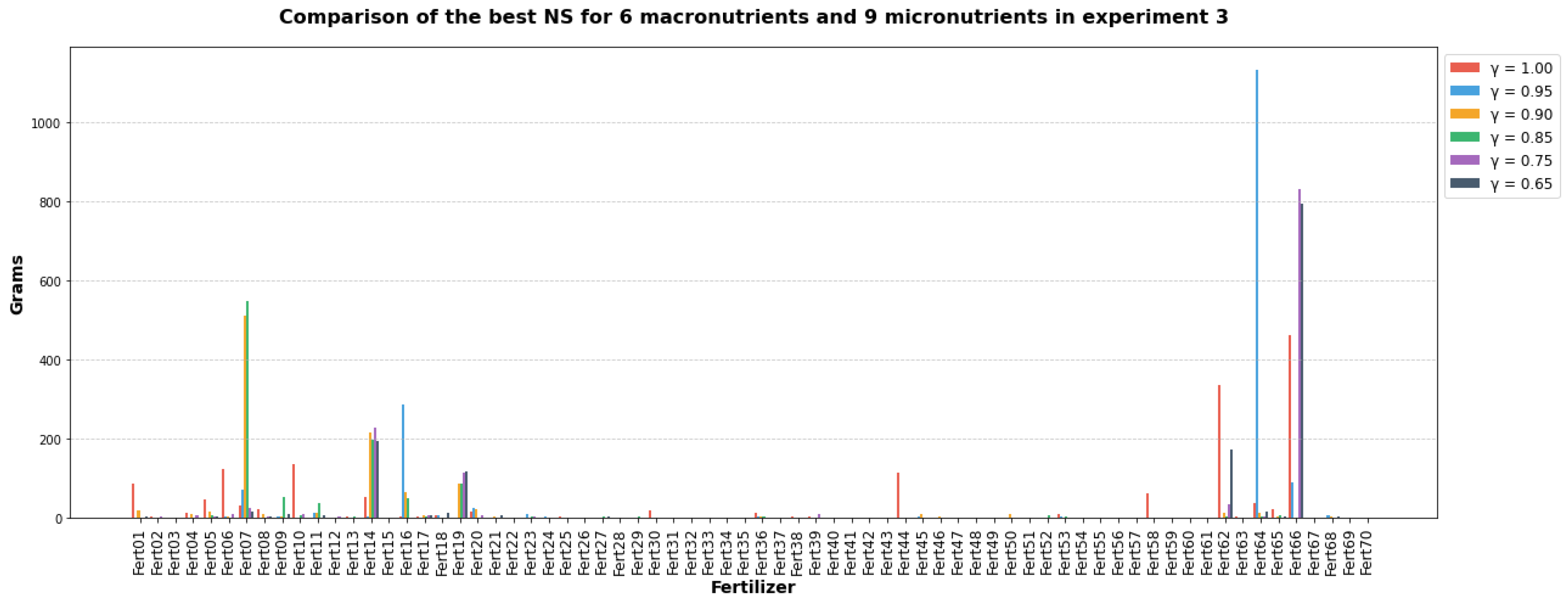
Figure 2 shows the quantities expressed in grams of each fertilizer in Table 2 required to formulate the best NS by applying FNSUSA from the first experimental configuration for different

γ

values.

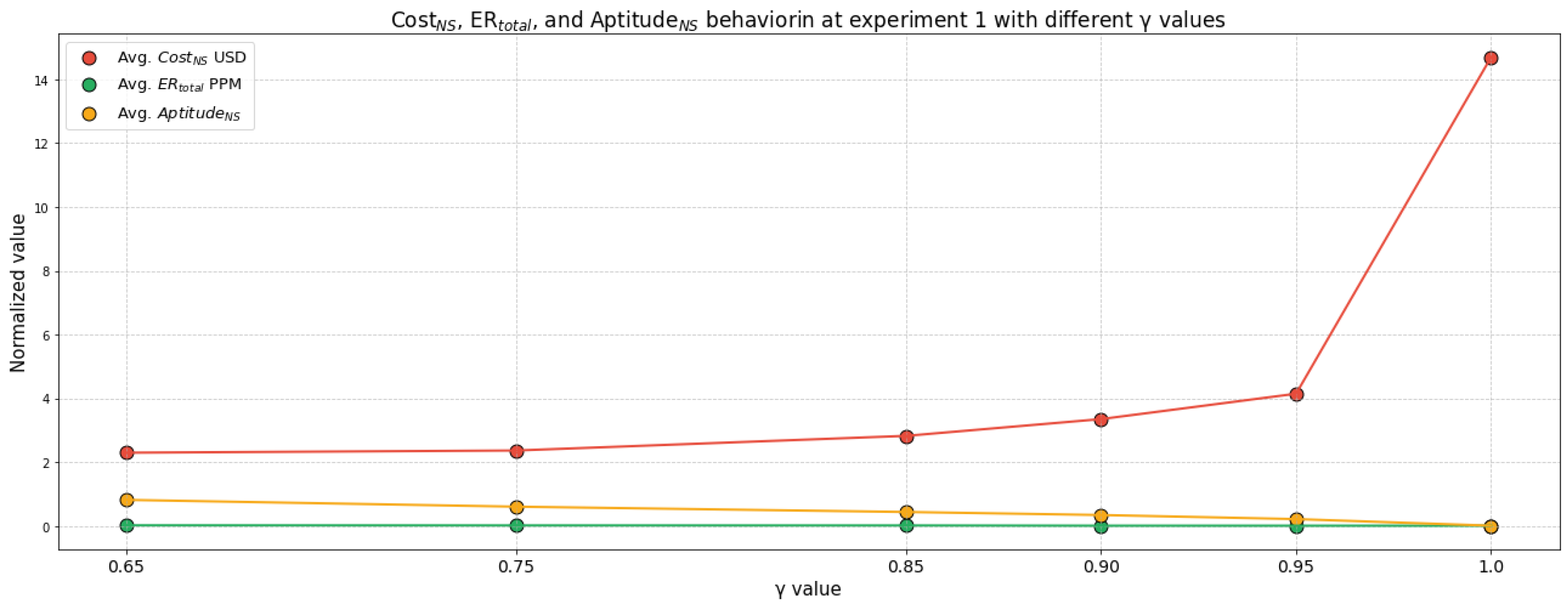
Figure 3 illustrates the behavior of the weighted averages of

C o s t_{N S}

,

R E_{t o t a l}

, and

A p t i t u d e_{N S}

of the NS as a function of the different

γ

values used in the ten runs of the FNSUSA for the first experimental configuration.

The behavior of the values in the graph shows the sensitivity of the algorithm to the trade-off between Nutrient

C o s t_{N S}

and total

C o s t_{N S}

,

R E_{t o t a l}

, demonstrating how increases in

γ

decrease

R E_{t o t a l}

at the expense of

C o s t_{N S}

.

5.2. Results Generated by FNSUSA in Configuration Targets 2

The second experimental configuration incorporates five chemical elements, Mg, S, and Ca, thus completing the six essential macronutrients required for optimal crop development. Two additional micronutrients, Fe and Zn, are also added, with FNSUSA finding it particularly challenging to achieve the target concentration of 0.5 PPM for Zn due to the low doses required, which make the formulation more complex to generate than the previous configuration.

Table 8 presents the results obtained in the ten runs of the FNSUSA corresponding to the second experimental configuration, highlighting in yellow the best NS based on the lowest value of

a p t i t u d e_{N S}

.

Table 9 shows the statistical data from the 60 FNSUSA runs generated with the results from Table 8 for the second experimental configuration, showing small standard deviation values, which demonstrates the repeatability of the FNSUSA.

Table 10 contains the quantitative data for the PPMs contained in the NS and their relative error from the best NS formulated using FNSUSA from Table 8.

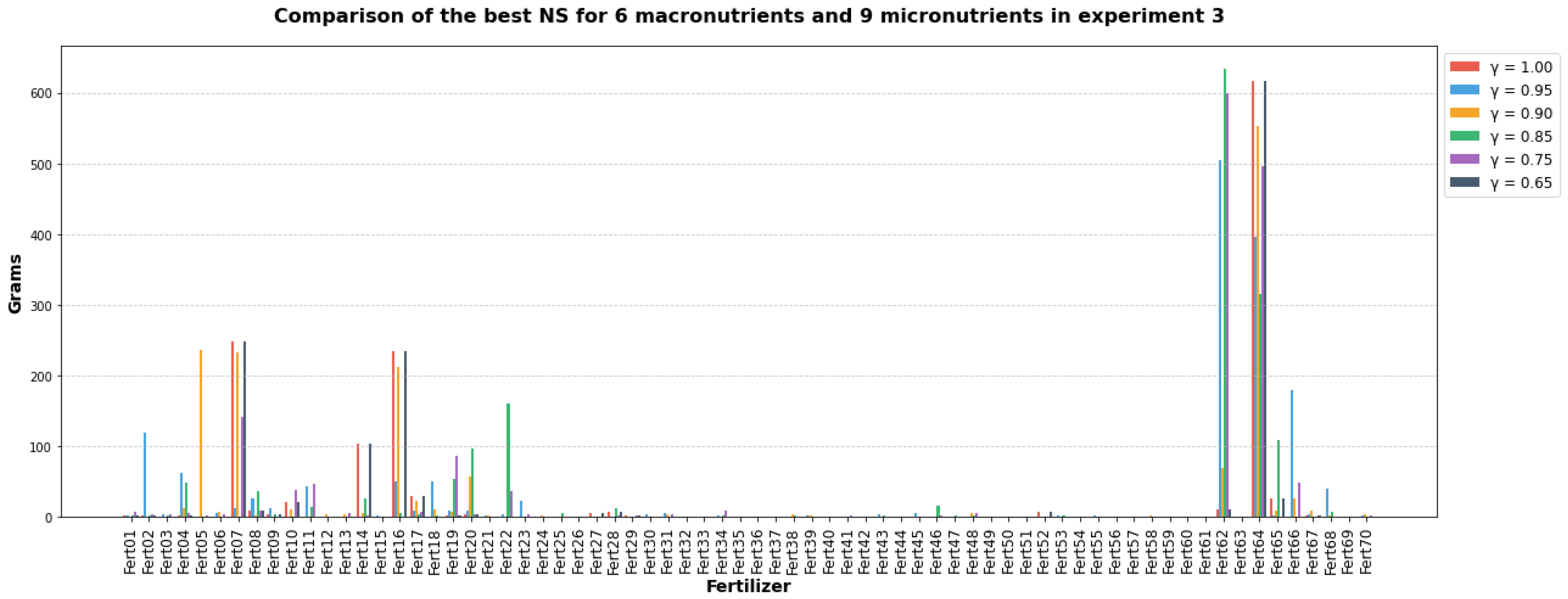
Figure 4 shows the quantities expressed in grams of each fertilizer in Table 2 required to formulate the best NS by applying FNSUSA from the second experimental configuration.

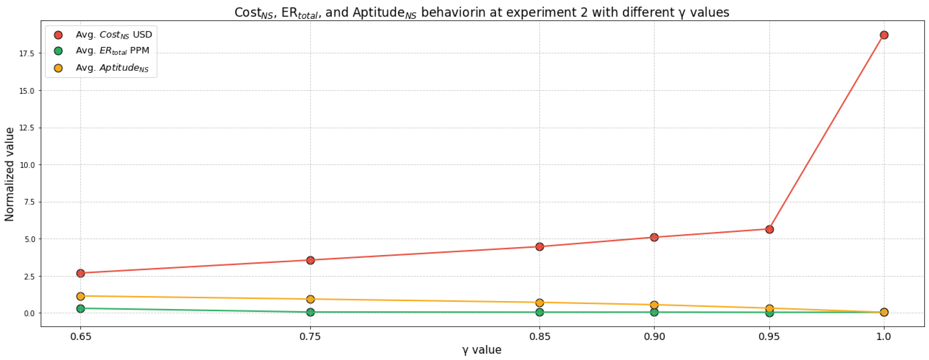
Figure 5 shows that

R E_{t o t a l}

decreases sharply as

γ

increases from

0.65

to

1.0

. This indicates that low

γ

values prioritize the balance between both objectives, while high values favor exclusively the minimization of

R E_{t o t a l}

,

C o s t_{N S}

shows an inverse trend in relation to

R E_{t o t a l}

. This behavior confirms that maximizing

A p t i t u d e_{N S}

in the formulation of target concentrations in PPM leads to an increase in the cost of NS.

5.3. Results Generated by FNSUSA in Configuration Targets 3

The third experimental configuration incorporates the micronutrients Cl, B, Cu, Mn, Mo, and Ni, completing the 15 nutrients required by crops. This configuration highlights the low target concentrations of Mo and Ni, set at

0.05

PPM in both cases, which pose an additional challenge for FNSUSA due to the need for extremely precise dosing to avoid both deficiencies and potential toxicity. The last configuration is the most difficult, as it requires very small PPM quantities to be achieved.

Table 11 presents the numerical values for

R e_{t o t a l}

,

C o s t_{N S}

, and

A p t i t u d e_{N S}

obtained in the ten runs of the FNSUSA algorithm for the third experimental configuration, which comprises 15 Nutrient chemical elements. These results correspond to the different weightings of the

γ

parameter; the best result obtained is highlighted in yellow, determined by the lowest value of

A p t i t u d e_{N S}

.

Finally, Table 12 shows similar standard deviation behavior, demonstrating the repeatability of the results generated by FNSUSA.

Table 13 contains the quantitative data for the PPMs contained in the NS and their relative error from the best NS formulated using FNSUSA from Table 11.

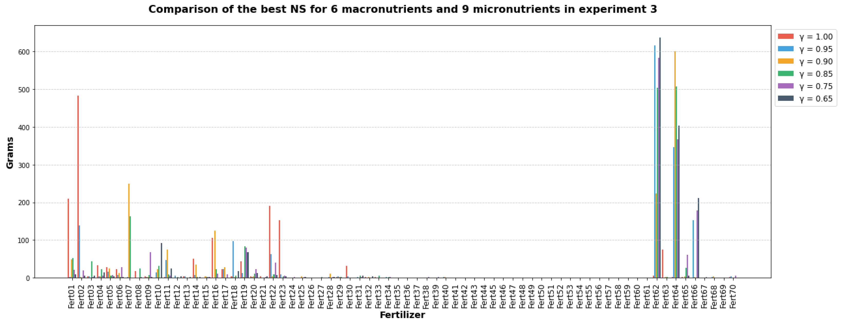
Figure 6 shows the quantities expressed in grams of each fertilizer in Table 2 required to formulate the best NS by applying FNSUSA from the third experimental configuration.

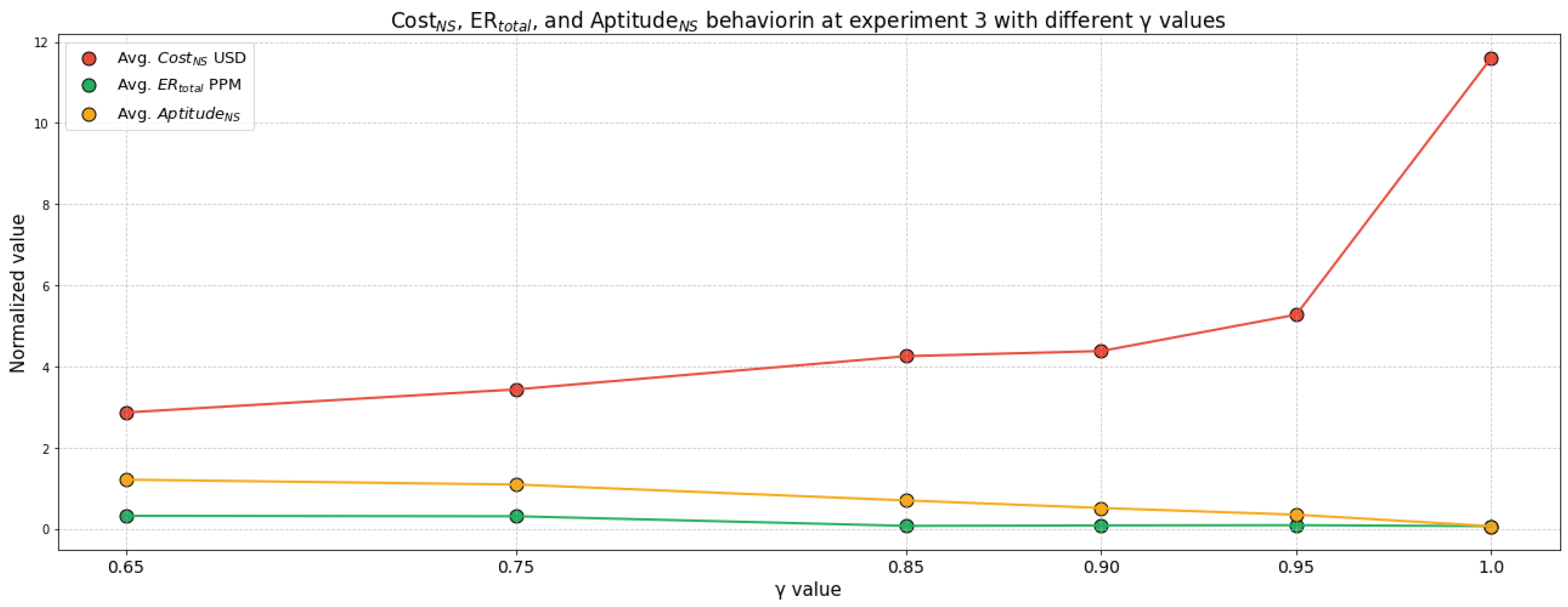
Figure 7 shows a similar behavior to the previous ones in relation to the cost and accuracy values that are weighted in the suitability of the NS. Low gamma values favor lower-cost solutions, accepting slight increases in the relative error of the target concentrations in PPM for macronutrients and micronutrients. In contrast, high gamma values prioritize reducing error in the formulation of the NS, which improves accuracy in meeting Nutrient objectives but increases the cost of the NS.

Figure 2, Figure 4 and Figure 6, which correspond to the best nutrient solutions (NS) with the lowest aptitude among the nine runs of each experimental configuration, show an increase in the number of fertilizers required for the formulation.

6. Conclusions

The FNSUSA algorithm efficiently optimizes fertilizer quantities to achieve target PPM concentrations of macronutrients and micronutrients in hydroponic crops. In the three experimental configurations (5, 10, and 15 nutrients), the average relative errors in ten runs with

γ = 1

are

0.01015, 0.0488,

and

0.06328,

respectively, demonstrating accuracy and revealing that complexity increases with the number of nutrients. The accuracy of FNSUSA in calculating fertilizer quantities for low PPM concentrations of micronutrients is noteworthy, especially in the third configuration, where it achieves minimal relative errors for Mo and Ni, both with targets of

0.05

PPM. Regarding cost, using

γ = 1

in the weighting prioritizes accuracy over cost, generating expensive NS with averages of USD 14.70, USD 18.75, and USD 11.61 across the three experimental configurations.

The use of

γ < 1

values significantly and consistently minimizes the cost of NS. In the first configuration with 5 nutrients, the average cost of 10 runs decreases from USD 14.70 with

γ = 1

to USD 2.30 with

γ = 0.65

. The second configuration with 10 nutrients, from USD 18.75 to USD 2.69, with the same

γ

values. Finally, in the third configuration with 15 target nutrients, the cost ranges from USD 11.61 to USD 2.87.

The analysis of weighting with values

γ < 1

significantly reduces the cost of NS without significantly increasing the absolute relative error in the target PPM concentrations of nutrients in the three experimental configurations. It is inferred that the most appropriate value for is

0.90 \leq γ \leq 1.0

. The value assigned to the

γ

factor helps farmers decide how much they are willing to sacrifice in accuracy in the NS relative to cost, depending on crop conditions.

7. Future Work

One aspect not explored in the reported results is the toxicity of the fertilizers used in the NS formulation. This will be addressed in future work by weighing toxicity against the cost and accuracy of the PPM concentrations for each nutrient. Another aspect to explore in future work, when adding the toxicity factor, is the normalization of the three variables to be balanced in order to avoid bias in the scale. An important aspect is the integration of the presented algorithm with real-time monitoring, which will enable more precise fertilization processes.

Author Contributions

Conceptualization, J.P.G.I. and F.J.C.d.l.R.; methodology, J.P.G.I. and F.J.C.d.l.R.; software, J.P.G.I. and A.J.R.R.; validation, J.P.G.I. and F.J.C.d.l.R.; formal analysis, J.P.G.I. and F.J.C.d.l.R.; investigation, J.P.G.I. and A.J.R.R.; writing—original draft preparation, J.P.G.I. and F.J.C.d.l.R.; writing—review and editing, J.P.G.I. and F.J.C.d.l.R.; supervision, F.J.C.d.l.R. All authors have read and agreed to the published version of the manuscript.

Funding

This research was funded by Tecnológico Nacional de México, Campus Zamora and by Secretaría de Ciencias, Humanidades, Tecnología e Innovación en Becas Nacionales grants.

Data Availability Statement

The data supporting the conclusions of this article will be made available by the authors on request.

Acknowledgments

It is important to thank the Institutions that made the development of this work possible by allocating resources of different kinds to carry it out. Secretaria de Ciencias, Humanidades, Tecnología e Innovación (SECIHTI), Tecnológico Nacional de México (TecNM), Instituto Tecnológico de Estudios Superiores de Zamora (ITESZ), and Centro de Investigaciones en Óptica A.C. (CIO).

Conflicts of Interest

The authors declare no conflicts of interest.

References

Awasthi, Y. Press “A” for Artificial Intelligence in Agriculture: A Review. Int. J. Inform. Vis. 2020, 4, 112–116. [Google Scholar] [CrossRef] [Scilit]
Ray, P.P. Internet of things for smart agriculture: Technologies, practices and future direction. J. Ambient. Intell. Smart Environ. 2017, 9, 395–420. [Google Scholar] [CrossRef] [Scilit]
FAO. Our Approach|Food Systems|Food and Agriculture Organization of the United Nations. 2023. Available online: http://www.fao.org/food-systems/our-approach/en/ (accessed on 1 December 2024).
Brown, P.D.; Cochrane, T.A.; Krom, T.D. Optimal on-farm irrigation scheduling with a seasonal water limit using simulated annealing. Agric. Water Manag. 2010, 97, 892–900. [Google Scholar] [CrossRef] [Scilit]
Dong, Y.; Zhao, C.; Yang, G.; Chen, L.; Wang, J.; Feng, H. Integrating a very fast simulated annealing optimization algorithm for crop leaf area index variational assimilation. Math. Comput. Model. 2013, 58, 877–885. [Google Scholar] [CrossRef] [Scilit]
Bai, Y.; Gao, J. Optimization of the nitrogen fertilizer schedule of maize under drip irrigation in Jilin, China, based on DSSAT and GA. Agric. Water Manag. 2021, 244, 106555. [Google Scholar] [CrossRef] [Scilit]
Gebbers, R.; Adamchuk, V.I. Precision agriculture and food security. Science 2010, 327, 828–831. [Google Scholar] [CrossRef] [Scilit] [PubMed]
Pierce, F.J.; Nowak, P. Aspects of precision agriculture. Adv. Agron. 1999, 67, 1–68. [Google Scholar]
Patrício, D.I.; Rieder, R. Computer vision and artificial intelligence in precision agriculture for grain crops: A systematic review. Comput. Electron. Agric. 2018, 153, 69–81. [Google Scholar] [CrossRef] [Scilit]
Bertsimas, D.; Tsitsiklis, J. Simulated Annealing. Stat. Sci. 1993, 8, 409–435. [Google Scholar] [CrossRef] [Scilit]
Nanni, L.; Maguolo, G.; Pancino, F. Insect pest image detection and recognition based on bio-inspired methods. Ecol. Inform. 2020, 57, 101089. [Google Scholar] [CrossRef] [Scilit]
Mundada, R.G.M. Detection and Classification of Pests in Greenhouse Using Image Processing. IOSR J. Electron. Commun. Eng. 2013, 5, 57–63. [Google Scholar] [CrossRef] [Scilit]
Fan, P.; Lang, G.; Yan, B.; Lei, X.; Guo, P.; Liu, Z.; Yang, F. A Method of Segmenting Apples Based on Gray-Centered RGB Color Space. Remote Sens. 2021, 13, 1211. [Google Scholar] [CrossRef] [Scilit]
Ni, X.; Li, C.; Jiang, H.; Takeda, F. Deep learning image segmentation and extraction of blueberry fruit traits associated with harvestability and yield. Hortic. Res. 2020, 7, 110. [Google Scholar] [CrossRef] [Scilit]
Guerra Ibarra, J.P.; Cuevas de la Rosa, F. Optimization of Color Dominance Factor by Greedy Algorithm for Leaves and Fruit Segmentation of Tomato Plants. In Proceedings of the Lecture Notes in Computer Science (Including Subseries Lecture Notes in Artificial Intelligence and Lecture Notes in Bioinformatics); Mezura-Montes, E., Acosta-Mesa, H.G., Carrasco-Ochoa, J.A., Martínez-Trinidad, J.F., Olvera-López, J.A., Eds.; Springer: Cham, Switzerland, 2024; Volume 14755 LNCS, pp. 200–209. [Google Scholar] [CrossRef] [Scilit]
Kuo, S.F.; Merkley, G.P.; Liu, C.W. Decision support for irrigation project planning using a genetic algorithm. Agric. Water Manag. 2000, 45, 243–266. [Google Scholar] [CrossRef] [Scilit]
Cropper, W.P.; Comerford, N.B. Optimizing simulated fertilizer additions using a genetic algorithm with a nutrient uptake model. Ecol. Model. 2005, 185, 271–281. [Google Scholar] [CrossRef] [Scilit]
Lu, J.; Yang, T.; Su, X.; Qi, H.; Yao, X.; Cheng, T.; Zhu, Y.; Cao, W.; Tian, Y. Monitoring leaf potassium content using hyperspectral vegetation indices in rice leaves. Precis. Agric. 2020, 21, 324–348. [Google Scholar] [CrossRef] [Scilit]
Qi, X.; Zhao, Y.; Huang, Y.; Wang, Y.; Qin, W.; Fu, W.; Guo, Y.; Ye, Y. A novel approach for nitrogen diagnosis of wheat canopies digital images by mobile phones based on histogram. Sci. Rep. 2021, 11, 13012. [Google Scholar] [CrossRef] [Scilit] [PubMed]
Li, M.; Li, J.; Mao, H.; Wu, Y. Diagnosis and detection of phosphorus nutrition level for Solanum lycopersicum based on electrical impedance spectroscopy. Biosyst. Eng. 2016, 143, 108–118. [Google Scholar] [CrossRef] [Scilit]
Sun, Y.; Tong, C.; He, S.; Wang, K.; Chen, L. Identification of Nitrogen, Phosphorus, and Potassium Deficiencies Based on Temporal Dynamics of Leaf Morphology and Color. Sustainability 2018, 10, 762. [Google Scholar] [CrossRef] [Scilit]
Tran, T.T.; Choi, J.W.; Le, T.T.H.; Kim, J.W. A comparative study of deep CNN in forecasting and classifying the macronutrient deficiencies on development of tomato plant. Appl. Sci. 2019, 9, 1601. [Google Scholar] [CrossRef] [Scilit]
Xu, X.; He, P.; Yang, F.; Ma, J.; Pampolino, M.F.; Johnston, A.M.; Zhou, W. Methodology of fertilizer recommendation based on yield response and agronomic efficiency for rice in China. Field Crop. Res. 2017, 206, 33–42. [Google Scholar] [CrossRef] [Scilit]
Ahmad, I.; Wajid, S.A.; Ahmad, A.; Cheema, M.J.M.; Judge, J. Optimizing irrigation and nitrogen requirements for maize through empirical modeling in semi-arid environment. Environ. Sci. Pollut. Res. 2019, 26, 1227–1237. [Google Scholar] [CrossRef] [Scilit]
Ahmed, U.; Lin, J.C.W.; Srivastava, G.; Djenouri, Y. A nutrient recommendation system for soil fertilization based on evolutionary computation. Comput. Electron. Agric. 2021, 189, 106407. [Google Scholar] [CrossRef] [Scilit]
Chen, C.; Wang, X.; Chen, H.; Wu, C.; Mafarja, M.; Turabieh, H. Towards precision fertilization: Multi-strategy grey wolf optimizer based model evaluation and yield estimation. Electronics 2021, 10, 2183. [Google Scholar] [CrossRef] [Scilit]
Mengel, K.; Kirkby, E. Principles of Vegetable Nutrition; Springer: Dordrecht, The Netherlands, 1978; Volume 15B,A. [Google Scholar]
Dimkpa, C.O.; Bindraban, P.S. Fortification of micronutrients for efficient agronomic production: A review. Agron. Sustain. Dev. 2016, 36, 7. [Google Scholar] [CrossRef] [Scilit]
Resh, H.M. Hydroponic Food Production: A Definitive Guidebook for the Advanced Home Gardener and the Commercial Hydroponic Grower. In Hydroponic Food Production; CRC Press: Boca Raton, FL, USA, 2022. [Google Scholar] [CrossRef] [Scilit]
Savvas, D.; Gruda, N. Application of soilless culture technologies in the modern greenhouse industry—A review. Eur. J. Hortic. Sci. 2018, 83, 280–293. [Google Scholar] [CrossRef] [Scilit]
Kirkpatrick, S.; Gelatt, C.D.; Vecchi, M.P. Optimization by simulated annealing. Science 1983, 220, 671–680. [Google Scholar] [CrossRef] [Scilit] [PubMed]
Mahdi, W.; Medjahed, S.A.; Ouali, M. Performance analysis of simulated annealing cooling schedules in the context of dense image matching. Comput. y Sist. 2017, 21, 493–501. [Google Scholar] [CrossRef] [Scilit]
Cámara de Comercio de Bogotá CCB. Manual Tomate; Cámara de Comercio de Bogotá: Bogotá, Colombia, 2015; pp. 1–56. [Google Scholar]
Steiner, A.A. A universal method for preparing nutrient solutions of a certain desired composition. Plant Soil 1961, 15, 134–154. [Google Scholar] [CrossRef] [Scilit]
Sonneveld, C.; Voogt, W. Plant Nutrition of Greenhouse Crops; Springer: Dordrecht, The Netherlands, 2009; pp. 1–431. [Google Scholar] [CrossRef] [Scilit]

Figure 1. Adaptation of the SA for formulation NS.

Figure 2. Distribution of the weight for each fertilizer available in Table 2 for the best NS generated for the first experimental configuration.

Figure 3. Behavior of

C o s t_{N S}

,

R E_{t o t a l}

, and

A p t i t u d e_{N S}

parameters with different

γ

values in experiment 1.

Figure 3. Behavior of

C o s t_{N S}

,

R E_{t o t a l}

, and

A p t i t u d e_{N S}

parameters with different

γ

values in experiment 1.

Figure 4. Distribution of the weight for each fertilizer available in Table 2 for the best NS generated for the second experimental configuration.

Figure 5. Behavior of

C o s t_{N S}

,

R E_{t o t a l}

, and

A p t i t u d e_{N S}

parameters with different

γ

values in experiment 2.

Figure 5. Behavior of

C o s t_{N S}

,

R E_{t o t a l}

, and

A p t i t u d e_{N S}

parameters with different

γ

values in experiment 2.

Figure 6. Distribution of the weight for each fertilizer available in Table 2 for the best NS generated for the third experimental configuration.

Figure 7. Behavior of cost, accuracy, and aptitude parameters with different

γ

values in experiment 3.

Figure 7. Behavior of cost, accuracy, and aptitude parameters with different

γ

values in experiment 3.

Table 1. List of 15 nutrients necessary for proper plant development.

Nutrients Necessary for Plant Development
No.	Element Name	Symbol	Category
1	Nitrogen	N	Macronutrients
2	Phosphorus	P
3	Potassium	K
4	Calcium	Ca
5	Magnesium	Mg
6	Sulfur	S
7	Iron	Fe	Micronutrients
8	Manganese	Mn
9	Copper	Cu
10	Zinc	Zn
11	Boron	B
12	Molybdenum	Mo
13	Chlorine	Cl
14	Nickel	Ni
15	Sodium	Na

Table 2. List of fertilizers to be considered for blending.

Fertilizer	Price Kg/USD	Chemical Formula	Molecular Weight g/mol
Calcium nitrate	2.75	$C a {(N O_{3})}_{2}$	164.06
Potassium nitrate	5.76	$K N O_{3}$	101.10
Diammonium phosphate	4.49	${(N H_{4})}_{2} H P O_{4}$	132.07
Ammonium nitrate	3.70	$N H_{4} N O_{3}$	80.05
Ammonium sulfate	3.17	${(N H_{4})}_{2} S O_{4}$	132.14
Urea	4.49	$C O {(N H_{2})}_{2}$	60.08
Phosphonite nitrate	2.91	$M g {(N O_{3})}_{2} \cdot 4 H_{2} O$	222.39
Monoammonium phosphate	1.43	$N H_{4} H_{2} P O_{4}$	115.02
Anhydrous ammonia	1.85	$N H_{3}$	17.05
Ammonium chloride	1.59	$N H_{4} C l$	53.51
Sodium nitrate	1.37	$N a N O_{3}$	84.99
Magnesium nitrate	1.37	$M g {(N O_{3})}_{2}$	148.31
Iron chelate	1.37	$C_{10} H_{12} F e N_{2} N a O_{8}$	367.05
Ferric nitrate	0.79	$F e {(N O_{3})}_{3}$	241.86
Zinc nitrate	1.27	$Z n {(N O_{3})}_{2}$	189.36
Zinc chelate	0.63	$C_{10} H_{12} N_{2} O_{8} N a_{2} Z n$	435.58
Copper nitrate	1.27	$C u {(N O_{3})}_{2}$	187.57
Copper chelate	2.38	$C_{10} H_{12} N_{2} O_{8} N a_{2} C u$	433.77
Manganese chelate	0.63	$C_{10} H_{12} N_{2} O_{8} N a_{2} M n$	389.13
Ammonium molybdate	6.08	${(N H_{4})}_{6} M o_{7} O_{24}$	1,169.86
Nickel nitrate	7.93	$N i {(N O_{3})}_{2}$	182.67
Chelated nickel	1.32	$C_{10} H_{12} N_{2} O_{8} N a_{2} N i$	428.88
Calcium potassium nitrate	6.34	$K C a {(N O_{3})}_{3}$	263.21
Magnesium potassium nitrate	0.42	$K M g {(N O_{3})}_{3}$	249.44
Monopotassium phosphate	1.37	$K H_{2} P O_{4}$	136.08
Phosphoric rock	6.34	$C a_{5} {(P O_{4})}_{3} F$	504.30
Superphosphate	7.93	$C a {(H_{2} P O_{4})}_{2} \cdot H_{2} O$	234
Phosphoric acid	5.55	$H_{3} P O_{4}$	97.99
Phosphorite	18.50	$C a_{5} {(P O_{4})}_{3} F$	504.30
Monosodium phosphate	60.78	$N a H_{2} P O_{4}$	117.96
Dipotassium phosphate	10.04	$K_{2} H P O_{4}$	174.13
Potassium sulfate	6.34	$K_{2} S O_{4}$	174.26
Potassium chloride	6.34	$K C l$	74.54
Potassium carbonate	3.70	$K_{2} C O_{3}$	138.16
Potassium hydroxide	7.03	$K O H$	56.09
Potassium magnesium sulfate	9.51	$K_{2} M g_{2} {(S O_{4})}_{3}$	414.99
Potassium borate	5.18	$K_{2} B_{4} O_{7}$	233.54
Calcium chloride	11.10	$C a C l_{2}$	113.01
Calcium borate	6.34	$C a_{2} B_{6} O_{11}$	221.08
Calcium molybdate	95.14	$C a M o O_{4}$	200.01
Magnesium sulfate	47.57	$M g S O_{4}$	120.37
Kieserite	58.14	$M g S O_{4} \cdot H_{2} O$	138.33
Magnesium chloride	7.93	$M g C l_{2} \cdot 6 H_{2} O$	203.30
Magnesium borate	31.71	$M g B_{4} O_{7}$	155.31
Ferrous sulfate	13.21	$F e S O_{4}$	151.91
Zinc sulfate	17.44	$Z n S O_{4}$	161.44
Anhydrous copper sulfate	12.05	$C u S O_{4}$	159.61
Copper sulfate pentahydrate	8.99	$C u S O_{4} \cdot 5 H_{2} O$	249.68
Manganese sulfate	11.63	$M n S O_{4}$	152.97
Nickel sulfate	17.81	$N i S O_{4}$	154.71
Ferric chloride	31.03	$F e C l_{3}$	162.19
Ferric oxide	21.14	$F e_{2} O_{3}$	159.65
Manganese chloride	25.37	$M n C l_{2}$	125.83
Manganese oxide	58.14	$M n O$	70.94
Manganese acetate	41.23	$M n {(C H_{3} C O O)}_{2} \cdot 4 H_{2} O$	245.08
Copper oxychloride	63.42	$C u_{2} {(O H)}_{3} C l$	213.56
Copper borate	74.00	$C u {(B O_{2})}_{2}$	149.17
Zinc chloride	68.71	$Z n C l_{2}$	136.28
Zinc borate	44.93	$Z n B_{4} O_{7}$	220.62
Sodium chloride	50.74	$N a C l$	58.43
Boric acid	79.28	$H_{3} B O_{3}$	61.81
Sodium borate	1.16	$N a_{2} B_{4} O_{7} \cdot 10 H_{2} O$	381.23
Sodium hydroxide	51.27	$N a O H$	39.98
Sodium carbonate	1.85	$N a_{2} C O_{3}$	105.99
Sodium molybdate	5.81	$N a_{2} M o O_{4}$	205.87
Molybdenum trioxide	1.59	$M o O_{3}$	143.94
Molybdenum tetraoxide	6.87	$M o O_{4}$	146.94
Nickel hydroxide	4.76	$N i {(O H)}_{2}$	92.69
Nickel chloride	11.63	$N i C l_{2}$	129.59

Table 3. Description of FNSUSA functions.

Description of FNSUSA Functions
Function	Purpose	Parameters	Returns
Load_fertilizer	Read chemical information about fertilizers from a database.	Does not receive parameters	F is a matrix containing the chemical information on fertilizers.
Generate_solution	Create an initial solution by assigning a number of grams of each fertilizer.	Low Limit ( $l l$ ), Upper Limit ( $u l$ ) and F.	Returns a vector S in the shape of the Equation (5).
Evaluate_aptitude	Evaluates the suitability of the NS it receives as a parameter.	S is the NS to be evaluated, O is the vector with the PPMs defined as the target, F and $γ$ is the weighting to be used.	Return the fitness of S, applying the Equation (12).
Modificate_solution	Apply a perturbation according to Equations (7) and (8) to create a candidate solution.	S is current NS, $ρ$ is the value to create the disturbance in NS and F	Returns a vector S in the shape of the Equation (5).
Generate_initial_temperature	Determine the initial temperature of SA by applying Equation (13).	Receive the randomly generated initial NS fitness values.	Returns the initial temperature of the SA.
Generate_cooling_factor	Establish the cooling factor of the SA by applying Equation (15).	Receives the initial temperature (t), final temperature ( $t_{f}$ ) of the system and number of desired iterations (I).	Returns the system cooling value $α$ .

Table 4. Target PPM in the experimental stage.

PPM Targets Tested in Tree Configuration Experiment for Test FNSUSA
Target PPM experiment 1
No.	Nutrient element	PPM
1	Potassium	250.00
2	Nitrogen	200.00
3	Phosphorus	60.00
4	Chlorine	5.00
5	Sodium	2.00
Target PPM experiment 2
No.	Nutrient element	PPM
6	Calcium	100.00
7	Magnesium	60.00
8	Sulfur	50.00
9	Iron	5.00
10	Zinc	0.50
Target PPM experiment 3
No.	Nutrient element	PPM
11	Copper	1.00
12	boron	0.50
13	Manganese	0.20
14	Molybdenum	0.05
15	Nickel	0.05

Table 5. Results generated by FNSUSA for experiment 1 with different

γ

values.

Table 5. Results generated by FNSUSA for experiment 1 with different

γ

values.

FNSUSA Results for Experiment 1
$γ = 0.65$			$γ = 0.75$			$γ = 0.85$
$R E_{t o t a l}$	$C o s t_{N S}$	$A p t i t u d e_{N S}$	$R E_{t o t a l}$	$C o s t_{N S}$	$A p t i t u d e_{N S}$	$R E_{t o t a l}$	$C o s t_{N S}$	$A p t i t u d e_{N S}$
0.04342	2.32	0.84022	0.01911	3.10	0.78933	0.01452	3.05	0.46984
0.02586	2.38	0.84981	0.02599	2.22	0.57449	0.01719	2.75	0.42711
0.01880	2.37	0.84172	0.01720	2.30	0.58790	0.01740	3.05	0.47229
0.01738	2.19	0.77780	0.02366	2.33	0.60025	0.01330	2.74	0.42231
0.01221	2.20	0.77794	0.01884	2.22	0.56913	0.02671	3.21	0.50420
0.01666	2.57	0.91033	0.01391	2.35	0.59793	0.02805	2.57	0.40934
0.00765	2.52	0.88697	0.02047	2.14	0.55035	0.01395	2.56	0.39586
0.03326	2.08	0.74962	0.02264	2.15	0.55448	0.03797	2.67	0.43277
0.01456	2.07	0.73396	0.02057	2.06	0.53043	0.00690	2.87	0.43637
0.03425	2.28	0.82026	0.00992	2.80	0.70744	0.00678	2.79	0.42426
$γ = 0.90$			$γ = 0.95$			$γ = 1$
$R E_{t o t a l}$	$C o s t_{N S}$	$A p t i t u d e_{N S}$	$R E_{t o t a l}$	$C o s t_{N S}$	$A p t i t u d e_{N S}$	$R E_{t o t a l}$	$C o s t_{N S}$	$A p t i t u d e_{N S}$
0.01275	3.26	0.33748	0.00575	4.93	0.25196	0.00707	16.80	0.00707
0.00727	2.92	0.29854	0.01039	3.40	0.17987	0.01201	8.96	0.01201
0.01485	2.86	0.29937	0.00773	4.53	0.23384	0.00500	12.69	0.00500
0.00800	3.13	0.32020	0.01444	4.03	0.21522	0.00660	26.23	0.00660
0.01248	3.76	0.38723	0.00702	3.71	0.19217	0.01179	4.35	0.01179
0.00655	4.29	0.43490	0.00823	4.73	0.24432	0.01265	13.00	0.01265
0.00756	2.98	0.30480	0.01001	4.27	0.22301	0.01720	21.44	0.01720
0.01127	2.93	0.30314	0.01408	3.22	0.17438	0.00929	20.17	0.00929
0.01649	4.04	0.41884	0.01662	4.55	0.24329	0.01105	14.54	0.01105
0.00680	3.35	0.34112	0.00814	4.10	0.21273	0.00881	8.77	0.00881

Table 6. Statistics for the results in Table 5.

FNSUSA Statistical Results for Experiment 1
Statistician	$γ = 0.65$			$γ = 0.75$			$γ = 0.85$
Statistician	$R E_{t o t a l}$	$C o s t_{N S}$	$A p t i t u d e_{N S}$	$R E_{t o t a l}$	$C o s t_{N S}$	$A p t i t u d e_{N S}$	$R E_{t o t a l}$	$C o s t_{N S}$	$A p t i t u d e_{N S}$
Mean	0.02241	2.29800	0.81886	0.01923	2.36700	0.60617	0.01828	2.82600	0.43944
Standard deviation	0.01030	0.15278	0.05249	0.00426	0.29650	0.07270	0.00892	0.19652	0.02974
Statistician	$γ = 0.90$			$γ = 0.95$			$γ = 1$
Statistician	$R E_{t o t a l}$	$C o s t_{N S}$	$A p t i t u d e_{N S}$	$R E_{t o t a l}$	$C o s t_{N S}$	$A p t i t u d e_{N S}$	$R E_{t o t a l}$	$C o s t_{N S}$	$A p t i t u d e_{N S}$
Mean	0.01040	3.35200	0.34456	0.01024	4.14700	0.21708	0.01015	14.69500	0.01015
Standard deviation	0.00329	0.45950	0.04633	0.00328	0.51358	0.02489	0.00322	5.99158	0.00322

Table 7. Comparison of the best solutions in experimental configuration 1 with different

γ

values.

Table 7. Comparison of the best solutions in experimental configuration 1 with different

γ

values.

Results of Experiment Configuration 1 with Different $γ$ Values
$γ = 0.65$					$γ = 0.75$					$γ = 0.85$
Nutrient	$P P M_{e}^{t}$	$P P M_{e}^{N S}$	$R E_{e}$	Total Grams	Nutrient	$P P M_{e}^{t}$	$P P M_{e}^{N S}$	$R E_{e}$	Total Grams	Nutrient	$P P M_{e}^{t}$	$P P M_{e}^{N S}$	$R E_{e}$	Total Grams
K	250.00	248.80174	0.00479	1383.92	K	250.00	249.47480	0.00210	1314.17	K	250.00	250.41620	0.00166	1036.79
N	200.00	199.91776	0.00041		N	200.00	200.37204	0.00186		N	200.00	199.76459	0.00118
P	60.00	59.93533	0.00108		P	60.00	59.23868	0.01269		P	60.00	59.96528	0.00058
Cl	5.00	5.03745	0.00749		Cl	5.00	5.00739	0.00148		Cl	5.00	5.04487	0.00897
Na	2.00	1.99849	0.00076		Na	2.00	1.99511	0.00245		Na	2.00	2.00313	0.00157
$γ = 0.90$					$γ = 0.95$					$γ = 1.0$
Nutrient	$P P M_{e}^{t}$	$P P M_{e}^{N S}$	$R E_{e}$	Total Grams	Nutrient	$P P M_{e}^{t}$	$P P M_{e}^{N S}$	$R E_{e}$	Total Grams	Nutrient	$P P M_{e}^{t}$	$P P M_{e}^{N S}$	$R E_{e}$	Total Grams
K	250.00	249.79577	0.00082	1059.49	K	250.00	250.52482	0.00210	1675.66	K	250.00	250.01255	0.00005	1645.63
N	200.00	200.39572	0.00198		N	200.00	200.15160	0.00076		N	200.00	199.85525	0.00072
P	60.00	60.04930	0.00082		P	60.00	59.92142	0.00131		P	60.00	59.85259	0.00246
Cl	5.00	5.00741	0.00148		Cl	5.00	4.95755	0.00849		Cl	5.00	4.99888	0.00022
Na	2.00	1.99562	0.00219		Na	2.00	2.00291	0.00145		Na	2.00	2.00309	0.00154

Table 8. Results generated by FNSUSA for experiment 2 with different

γ

values.

Table 8. Results generated by FNSUSA for experiment 2 with different

γ

values.

FNSUSA Results for Experiment 2
$γ = 0.65$			$γ = 0.75$			$γ = 0.85$
$R E_{t o t a l}$	$C o s t_{N S}$	$A p t i t u d e_{N S}$	$R E_{t o t a l}$	$C o s t_{N S}$	$A p t i t u d e_{N S}$	$R E_{t o t a l}$	$C o s t_{N S}$	$A p t i t u d e_{N S}$
0.60470	2.51	1.27155	0.11989	4.11	1.11742	0.04945	5.40	0.85203
0.22999	3.23	1.27999	0.03172	3.30	0.84879	0.05056	4.01	0.64447
0.98120	1.75	1.25028	0.02862	3.26	0.83646	0.03479	5.86	0.90858
0.13349	2.72	1.03877	0.05164	4.49	1.16123	0.03778	3.76	0.59611
0.24232	2.79	1.13401	0.04425	3.49	0.90569	0.03002	4.03	0.63002
0.17508	2.65	1.04130	0.06566	3.19	0.84675	0.11761	4.75	0.81247
0.19149	2.67	1.05897	0.06802	3.29	0.87352	0.02617	4.89	0.75574
0.22816	2.72	1.10030	0.08501	4.22	1.11876	0.07486	3.83	0.63813
0.16763	2.90	1.12396	0.02720	3.08	0.79040	0.04227	3.75	0.59843
0.11744	2.91	1.09484	0.04601	3.13	0.81701	0.01486	4.33	0.66213
$γ = 0.90$			$γ = 0.95$			$γ = 1$
$R E_{t o t a l}$	$C o s t_{N S}$	$A p t i t u d e_{N S}$	$R E_{t o t a l}$	$C o s t_{N S}$	$A p t i t u d e_{N S}$	$R E_{t o t a l}$	$C o s t_{N S}$	$A p t i t u d e_{N S}$
0.06194	4.92	0.54775	0.08228	4.94	0.32517	0.04136	11.70	0.04136
0.05046	3.89	0.43441	0.03319	6.29	0.34603	0.04214	13.98	0.04214
0.02246	4.96	0.51621	0.03548	5.38	0.30271	0.04285	21.32	0.04285
0.05623	7.11	0.76161	0.03922	4.89	0.28176	0.05242	15.19	0.05242
0.04325	4.84	0.52293	0.04244	7.14	0.39732	0.04054	16.23	0.04054
0.04626	4.94	0.53563	0.03359	4.89	0.27641	0.02618	14.57	0.02618
0.04166	6.19	0.65649	0.03645	7.06	0.38763	0.03076	8.91	0.03076
0.05424	4.15	0.46382	0.03671	4.16	0.24287	0.04114	21.94	0.04114
0.02563	5.06	0.52907	0.01870	4.20	0.22777	0.04488	25.48	0.04488
0.07324	4.85	0.55092	0.03405	7.56	0.41035	0.04651	38.15	0.04651

Table 9. Statistics for the results in Table 8.

FNSUSA Statistical Results for Experiment 2
Statistician	$γ = 0.65$			$γ = 0.75$			$γ = 0.85$
Statistician	$R E_{t o t a l}$	$C o s t_{N S}$	$A p t i t u d e_{N S}$	$R E_{t o t a l}$	$C o s t_{N S}$	$A p t i t u d e_{N S}$	$R E_{t o t a l}$	$C o s t_{N S}$	$A p t i t u d e_{N S}$
Mean	0.30715	2.68500	1.13940	0.05680	3.55600	0.93160	0.04784	4.46100	0.70981
Standard deviation	0.24785	0.34558	0.08503	0.02625	0.46617	0.12881	0.02660	0.66796	0.10259
Statistician	$γ = 0.90$			$γ = 0.95$			$γ = 1$
Statistician	$R E_{t o t a l}$	$C o s t_{N S}$	$A p t i t u d e_{N S}$	$R E_{t o t a l}$	$C o s t_{N S}$	$A p t i t u d e_{N S}$	$R E_{t o t a l}$	$C o s t_{N S}$	$A p t i t u d e_{N S}$
Mean	0.04754	5.09100	0.55188	0.03921	5.65100	0.31980	0.04088	18.74700	0.04088
Standard deviation	0.01401	0.84225	0.08496	0.01480	1.14100	0.05842	0.00678	7.65275	0.00678

Table 10. Comparison of the best solutions in experimental configuration 2 with different

γ

values.

Table 10. Comparison of the best solutions in experimental configuration 2 with different

γ

values.

Results of Experiment Configuration 2 with Different $γ$ Values
$γ = 0.65$					$γ = 0.75$					$γ = 0.85$
Nutrient	$P P M_{e}^{t}$	$P P M_{e}^{N S}$	$R E_{e}$	Total Grams	Nutrient	$P P M_{e}^{t}$	$P P M_{e}^{N S}$	$R E_{e}$	Total Grams	Nutrient	$P P M_{e}^{t}$	$P P M_{e}^{N S}$	$R E_{e}$	Total Grams
K	250.00	224.66522	0.10134	1341.73	K	250.00	247.88492	0.00846	1588.11	K	250.00	248.97781	0.00409	1574.22
N	200.00	199.06995	0.00465		N	200.00	200.08801	0.00044		N	200.00	200.12032	0.00060
Ca	100.00	100.73784	0.00738		Ca	100.00	100.21355	0.00214		Ca	100.00	100.55874	0.00559
P	60.00	59.99536	0.00008		P	60.00	59.83592	0.00273		P	60.00	60.43355	0.00723
Mg	60.00	60.76362	0.01273		Mg	60.00	60.38002	0.00633		Mg	60.00	60.71300	0.01188
S	50.00	49.94364	0.00113		S	50.00	49.86168	0.00277		S	50.00	50.07246	0.00145
Cl	5.00	4.99542	0.00092		Cl	5.00	5.00080	0.00016		Cl	5.00	4.99055	0.00189
Fe	5.00	5.00486	0.00097		Fe	5.00	4.99793	0.00041		Fe	5.00	4.98875	0.00225
Na	2.00	1.99306	0.00347		Na	2.00	2.00299	0.00149		Na	2.00	2.00542	0.00271
Zn	0.50	0.49957	0.00086		Zn	0.50	0.49882	0.00236		Zn	0.50	0.50007	0.00014
$γ = 0.90$					$γ = 0.95$					$γ = 1.0$
Nutrient	$P P M_{e}^{t}$	$P P M_{e}^{N S}$	$R E_{e}$	Total Grams	Nutrient	$P P M_{e}^{t}$	$P P M_{e}^{N S}$	$R E_{e}$	Total Grams	Nutrient	$P P M_{e}^{t}$	$P P M_{e}^{N S}$	$R E_{e}$	Total Grams
K	250.00	249.33045	0.00268	1523.58	K	250.00	250.14301	0.00057	1614.15	K	250.00	249.89713	0.00041	1579.20
N	200.00	198.35980	0.00820		N	200.00	200.15482	0.00077		N	200.00	198.76812	0.00616
Ca	100.00	100.07606	0.00076		Ca	99.42206	99.95805	0.00042		Ca	99.42206	99.42206	0.00578
P	60.00	59.70952	0.00484		P	60.00	60.03713	0.00062		P	60.00	60.24351	0.00406
Mg	60.00	60.07460	0.00124		Mg	60.00	60.18923	0.00315		Mg	60.00	59.94201	0.00097
S	50.00	50.66004	0.01320		S	50.00	50.50481	0.01010		S	50.00	49.75296	0.00494
Cl	5.00	5.05585	0.01117		Cl	5.00	5.00373	0.00075		Cl	5.00	4.99174	0.00165
Fe	5.00	5.01955	0.00391		Fe	5.00	4.99591	0.00082		Fe	5.00	5.00451	0.00090
Na	2.00	1.99707	0.00147		Na	2.00	1.99952	0.00024		Na	2.00	2.00086	0.00043
Zn	0.50	0.49851	0.00298		Zn	0.50	0.50066	0.00133		Zn	0.50	0.50044	0.00089

Table 11. Results generated by FNSUSA for experiment 3 with different gamma values.

FNSUSA Results for Experiment 3
$γ = 0.65$			$γ = 0.75$			$γ = 0.85$
$R E_{t o t a l}$	$C o s t_{N S}$	$A p t i t u d e_{N S}$	$R E_{t o t a l}$	$C o s t_{N S}$	$A p t i t u d e_{N S}$	$R E_{t o t a l}$	$C o s t_{N S}$	$A p t i t u d e_{N S}$
0.47263	2.84	1.30121	1.35238	2.08	1.53428	0.04818	3.60	0.58095
1.12610	2.84	1.72597	0.22389	3.13	0.95042	0.03465	5.47	0.84995
0.50481	2.67	1.26263	0.09559	3.39	0.91919	0.05505	4.57	0.73229
0.09948	2.94	1.09366	0.07323	3.11	0.83242	0.08955	3.62	0.61912
0.19599	2.88	1.13539	0.51630	3.44	1.24723	0.09121	4.75	0.79003
0.22675	2.74	1.10639	0.12678	4.97	1.33758	0.09821	4.07	0.69398
0.10397	3.09	1.14908	0.11581	3.46	0.95186	0.06076	4.97	0.79715
0.22105	2.65	1.07118	0.05846	4.56	1.18385	0.06978	4.29	0.70281
0.06690	3.31	1.20199	0.24448	3.11	0.96086	0.08280	3.83	0.64488
0.15597	2.70	1.04638	0.26569	3.09	0.97177	0.06863	3.36	0.56234
$γ = 0.90$			$γ = 0.95$			$γ = 1$
$R E_{t o t a l}$	$C o s t_{N S}$	$A p t i t u d e_{N S}$	$R E_{t o t a l}$	$C o s t_{N S}$	$A p t i t u d e_{N S}$	$R E_{t o t a l}$	$C o s t_{N S}$	$A p t i t u d e_{N S}$
0.07303	3.71	0.43673	0.13816	5.03	0.38275	0.03185	13.71	0.03185
0.08503	5.21	0.59753	0.06252	3.79	0.24889	0.04005	16.11	0.04005
0.04997	5.45	0.58997	0.08094	5.12	0.33289	0.03077	11.12	0.03077
0.09041	4.01	0.48237	0.06225	6.97	0.40764	0.08526	12.37	0.08526
0.12209	5.38	0.64788	0.14817	5.55	0.41826	0.05145	14.30	0.05145
0.08501	3.91	0.46751	0.07613	5.74	0.35932	0.05128	13.09	0.05128
0.07745	3.85	0.45471	0.08280	4.57	0.30716	0.06211	10.07	0.06211
0.06604	3.87	0.44644	0.05842	5.87	0.34900	0.08875	8.07	0.08875
0.08297	3.39	0.41367	0.08232	5.46	0.35120	0.10472	12.38	0.10472
0.07895	5.01	0.57206	0.07485	4.66	0.30411	0.08653	4.86	0.08653

Table 12. Statistics for the results in Table 11.

FNSUSA Statistical Results for Experiment 3
Statistician	$γ = 0.65$			$γ = 0.75$			$γ = 0.85$
Statistician	$R E_{t o t a l}$	$C o s t_{N S}$	$A p t i t u d e_{N S}$	$R E_{t o t a l}$	$C o s t_{N S}$	$A p t i t u d e_{N S}$	$R E_{t o t a l}$	$C o s t_{N S}$	$A p t i t u d e_{N S}$
Mean	0.31737	2.86600	1.20939	0.30726	3.43400	1.08895	0.06988	4.25300	0.69735
Standard deviation	0.29035	0.18656	0.18014	0.35411	0.73136	0.20381	0.01866	0.61652	0.08726
Statistician	$γ = 0.90$			$γ = 0.95$			$γ = 1$
Statistician	$R E_{t o t a l}$	$C o s t_{N S}$	$A p t i t u d e_{N S}$	$R E_{t o t a l}$	$C o s t_{N S}$	$A p t i t u d e_{N S}$	$R E_{t o t a l}$	$C o s t_{N S}$	$A p t i t u d e_{N S}$
Mean	0.08110	4.37900	0.51089	0.08666	5.27600	0.34612	0.06328	11.60800	0.06328
Standard deviation	0.01673	0.71086	0.07460	0.02817	0.78147	0.04617	0.02385	2.95362	0.02385

Table 13. Comparison of the best solutions in experimental configuration 3 with different

γ

values.

Table 13. Comparison of the best solutions in experimental configuration 3 with different

γ

values.

Results of Experiment Configuration 3 with Different $γ$ Values
$γ = 0.65$					$γ = 0.75$					$γ = 0.85$
Nutrient	$P P M_{e}^{t}$	$P P M_{e}^{N S}$	$R E_{e}$	Total Grams	Nutrient	$P P M_{e}^{t}$	$P P M_{e}^{N S}$	$R E_{e}$	Total Grams	Nutrient	$P P M_{e}^{t}$	$P P M_{e}^{N S}$	$R E_{e}$	Total Grams
K	250.00	227.92070	0.08832	1562.00	K	250.00	248.18028	0.00728	1550.55	K	250.00	247.15375	0.01138	1566.94
N	200.00	200.84282	0.00421		N	200.00	200.06876	0.00034		N	200.00	200.13222	0.00066
Ca	100.00	99.61625	0.00384		Ca	100.00	100.10421	0.00104		Ca	100.00	99.68153	0.00318
P	60.00	60.33785	0.00563		P	60.00	60.36842	0.00614		P	60.00	59.34051	0.01099
Mg	60.00	60.53141	0.00886		Mg	60.00	59.69300	0.00512		Mg	60.00	60.50506	0.00842
S	50.00	50.28611	0.00572		S	50.00	49.66624	0.00668		S	50.00	49.97250	0.00055
Cl	5.00	5.00208	0.00042		Cl	5.00	5.07543	0.01509		Cl	5.00	5.00825	0.00165
Fe	5.00	4.93982	0.01204		Fe	5.00	4.99958	0.00008		Fe	5.00	5.00015	0.00003
Na	2.00	1.99827	0.00087		Na	2.00	1.97624	0.01188		Na	2.00	2.00716	0.00358
B	1.00	0.99621	0.00379		B	1.00	1.00317	0.00317		B	1.00	0.99174	0.00826
Cu	0.50	0.49602	0.00795		Cu	0.50	0.49976	0.00049		Cu	0.50	0.50054	0.00108
Zn	0.50	0.50059	0.00118		Zn	0.50	0.50151	0.00303		Zn	0.50	0.49780	0.00440
Mn	0.20	0.19967	0.00166		Mn	0.20	0.19964	0.00182		Mn	0.20	0.19970	0.00149
Mo	0.05	0.05017	0.00331		Mo	0.05	0.05023	0.00461		Mo	0.05	0.04960	0.00802
Ni	0.05	0.04959	0.00817		Ni	0.05	0.05032	0.00646		Ni	0.05	0.04984	0.00317
$γ = 0.90$					$γ = 0.95$					$γ = 1.0$
Nutrient	$P P M_{e}^{t}$	$P P M_{e}^{N S}$	$R E_{e}$	Total Grams	Nutrient	$P P M_{e}^{t}$	$P P M_{e}^{N S}$	$R E_{e}$	Total Grams	Nutrient	$P P M_{e}^{t}$	$P P M_{e}^{N S}$	$R E_{e}$	Total Grams
K	250.00	250.99282	0.00397	1509.60	K	250.00	249.62558	0.00150	1517.86	K	250.00	249.62558	0.00150	1517.86
N	200.00	199.35386	0.00323		N	200.00	199.85667	0.00072		N	200.00	199.85667	0.00072
Ca	100.00	100.55600	0.00556		Ca	100.00	100.02876	0.00029		Ca	100.00	100.02876	0.00029
P	60.00	59.95042	0.00083		P	60.00	60.00369	0.00006		P	60.00	60.00369	0.00006
Mg	60.00	60.48324	0.00805		Mg	60.00	59.88071	0.00199		Mg	60.00	59.88071	0.00199
S	50.00	49.73301	0.00534		S	50.00	49.98011	0.00040		S	50.00	49.98011	0.00040
Cl	5.00	4.98230	0.00354		Cl	5.00	5.01926	0.00385		Cl	5.00	5.01926	0.00385
Fe	5.00	5.04406	0.00881		Fe	5.00	5.00682	0.00136		Fe	5.00	5.00682	0.00136
Na	2.00	1.98538	0.00731		Na	2.00	2.01088	0.00544		Na	2.00	2.01088	0.00544
B	1.00	0.99443	0.00557		B	1.00	0.99157	0.00843		B	1.00	0.99157	0.00843
Cu	0.50	0.49663	0.00674		Cu	0.50	0.50053	0.00106		Cu	0.50	0.50053	0.00106
Zn	0.50	0.50435	0.00871		Zn	0.50	0.50017	0.00033		Zn	0.50	0.50017	0.00033
Mn	0.20	0.20081	0.00404		Mn	0.20	0.20031	0.00153		Mn	0.20	0.20031	0.00153
Mo	0.05	0.05021	0.00412		Mo	0.05	0.05003	0.00067		Mo	0.05	0.05003	0.00067
Ni	0.05	0.05035	0.00697		Ni	0.05	0.05016	0.00314		Ni	0.05	0.05016	0.00314

Disclaimer/Publisher’s Note: The statements, opinions and data contained in all publications are solely those of the individual author(s) and contributor(s) and not of MDPI and/or the editor(s). MDPI and/or the editor(s) disclaim responsibility for any injury to people or property resulting from any ideas, methods, instructions or products referred to in the content.

Share and Cite

MDPI and ACS Style

Guerra Ibarra, J.P.; Cuevas de la Rosa, F.J.; Rocha Rocha, A.J. Formulation of Nutrient Solutions Using Simulated Annealing. Agriculture 2026, 16, 449. https://doi.org/10.3390/agriculture16040449

AMA Style

Guerra Ibarra JP, Cuevas de la Rosa FJ, Rocha Rocha AJ. Formulation of Nutrient Solutions Using Simulated Annealing. Agriculture. 2026; 16(4):449. https://doi.org/10.3390/agriculture16040449

Chicago/Turabian Style

Guerra Ibarra, Juan Pablo, Francisco Javier Cuevas de la Rosa, and Aaron Junior Rocha Rocha. 2026. "Formulation of Nutrient Solutions Using Simulated Annealing" Agriculture 16, no. 4: 449. https://doi.org/10.3390/agriculture16040449

APA Style

Guerra Ibarra, J. P., Cuevas de la Rosa, F. J., & Rocha Rocha, A. J. (2026). Formulation of Nutrient Solutions Using Simulated Annealing. Agriculture, 16(4), 449. https://doi.org/10.3390/agriculture16040449

Note that from the first issue of 2016, this journal uses article numbers instead of page numbers. See further details here.

Article Menu

Formulation of Nutrient Solutions Using Simulated Annealing

Abstract

1. Introduction

2. Related Works

3. Materials and Methods

3.1. Plant Nutrition

3.2. Algorithm for Formulating Nutritious Solutions Using Simulated Annealing

3.3. Development Environment and Computer Specifications

4. Experimentation

4.1. Characteristics of Selected Crop for the Step of Experimentation

4.2. Results of FNSUSA

5. Results

5.1. Results Generated by FNSUSA in Configuration Targets 1

5.2. Results Generated by FNSUSA in Configuration Targets 2

5.3. Results Generated by FNSUSA in Configuration Targets 3

6. Conclusions

7. Future Work

Author Contributions

Funding

Data Availability Statement

Acknowledgments

Conflicts of Interest

References

Share and Cite

Article Metrics

Article Access Statistics

Further Information

Guidelines

MDPI Initiatives

Follow MDPI