Calibration of DEM Contact Parameters for Fresh Goji Berries Using an OLHS-BP Neural Network-MIGA Framework

Abstract

Accurate discrete element method (DEM) simulation of postharvest goji berry processing equipment is limited by the difficulty of directly measuring microscopic contact parameters. This study proposes an integrated DEM parameter calibration framework for fresh goji berries by combining optimal Latin hypercube sampling (OLHS), a back-propagation (BP) neural network, and a multi-island genetic algorithm (MIGA). Fresh ‘Ningqi No. 7’ goji berries were used as the test material. Physical experiments determined particle density (840.47 kg/m³), elastic modulus (1.1352 × 10⁵ Pa), Poisson’s ratio (0.32), shear modulus (4.3 × 10⁴ Pa), average angle of repose (AoR, 32.87 ± 2.20°), and pile height (Height, 65.57 ± 4.10 mm). Based on optimal Latin hypercube sampling (OLHS), 150 virtual DEM experiments were designed. Six contact parameters, including the coefficients of restitution, static friction, and rolling friction for goji–goji and goji–PVC contacts, were used as inputs, while AoR and Height were selected as macroscopic responses. A BP neural network was trained to establish the nonlinear mapping between microscopic parameters and macroscopic responses, and MIGA was used to optimize the surrogate model globally. The BP model achieved test-set R² values of 0.9415 and 0.9429, and RMSE values of 1.0633 and 0.8447 for AoR and Height, respectively. MIGA yielded 90 feasible parameter sets, with relative errors between predicted and DEM-simulated values below 5% at all validation points. Physical validation confirmed that the representative solution reproduced the macroscopic piling behavior of goji berries, providing effective DEM parameters for postharvest equipment simulation and optimization.

1. Introduction

The discrete element method (DEM) has been widely applied to the simulation of granular flows in engineering and agricultural systems because it can resolve particle-scale dynamics and bulk behavior from the principles of contact mechanics [1,2,3]. In agricultural engineering, contact mechanics provides a fundamental basis for understanding interactions between biological materials, machinery, and granular media. During harvesting, conveying, and processing, agricultural materials experience contact, friction, and deformation, which significantly affect material behavior and equipment performance. For irregular and deformable biological materials, such as fresh fruits and vegetables, accurate characterization of microscopic contact parameters is essential for reliable DEM simulations and agricultural equipment optimization. However, the accuracy of DEM simulations depends critically on appropriate microscopic contact parameters, including the coefficient of restitution, static friction coefficient, and rolling friction coefficient. For many irregular and soft particles, these parameters cannot be measured directly and must therefore be calibrated [4,5]. Conventional trial-and-error calibration is laborious and time-consuming, and its practicality decreases rapidly as the dimensionality of the parameter space increases [6].

Recent studies have sought to improve DEM parameter calibration through more systematic strategies. Machine-learning surrogate models have been introduced to replace repeated DEM simulations and thereby reduce computational cost. For example, iterative surrogate calibration based on random forests has been used to reproduce the macroscopic responses of cohesive materials with high accuracy [7]. Neural-network models have also been used to approximate the micro-macro relationships in DEM and assist parameter identification [8]. In particular, BP neural networks have been applied to link input parameters with dynamic flow behavior, showing higher efficiency than direct search methods [9]. In addition, design-of-experiment strategies, such as Latin hypercube sampling, can improve the diversity of training datasets and enhance the generalization capacity of surrogate models.

Evolutionary algorithms have also attracted increasing attention in DEM parameter calibration. Genetic algorithms and their variants can perform gradient-free global optimization and have been successfully applied in multi-objective calibration frameworks [9].

Despite these advances, DEM parameter calibration for flexible agricultural particles, particularly fresh goji berries, remains underexplored. Fresh goji berries are characterized by an irregular ellipsoidal shape, high moisture content, and low mechanical stiffness, all of which complicate parameter measurement and reduce simulation accuracy. Calibration methods developed for beans and cereal grains cannot be directly transferred to soft, deformable particles [10]. A recent study calibrated DEM parameters for fresh goji berries by combining physical experiments with Design-Expert optimization, mainly using heap formation and free-fall tests [11]. However, that optimization process relied on response surface regression and did not fully exploit surrogate modeling and evolutionary optimization.

Compared with previous calibration approaches based primarily on response surface regression, this study integrates OLHS, a BP neural network, and MIGA into an integrated calibration framework for fresh goji berries with irregular morphology and flexible characteristics. The novelty of this framework lies in the integration of optimized sampling, nonlinear surrogate modeling, and global evolutionary optimization within a unified DEM calibration process. Compared with conventional trial-and-error and response-surface-based calibration approaches, this framework reduces dependence on repeated DEM simulations and manual parameter adjustment by establishing an efficient nonlinear mapping between microscopic contact parameters and macroscopic responses.

The objective of this study is not to develop a new optimization algorithm, but to establish an integrated calibration strategy for the microscopic contact parameter calibration of fresh goji berries. Physical experiments were used to determine AoR and Height as macroscopic response indices. OLHS was then used to design uniformly distributed DEM sampling points and generate training data. A BP neural network surrogate model was trained to approximate the nonlinear mapping between microscopic contact parameters and macroscopic responses, and MIGA was used to globally optimize the microscopic contact parameters. Finally, DEM simulations were performed to validate the optimized parameter sets and confirm that they reliably reproduced the experimentally observed macroscopic behavior.

2. Materials and Methods

2.1. Experimental Materials

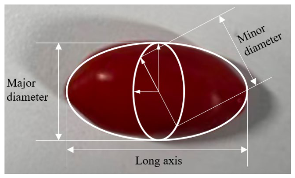
Fresh ‘Ningqi No. 7’ goji berries from Jingyuan County, Gansu Province, China, were used in this study. All physical experiments were conducted from August to September 2025. Fifty fresh goji berries were randomly selected from the collected samples. The selected goji berries were visually mature, characterized by uniform red color, intact surface, and absence of visible mechanical damage or decay. Before testing, the samples were stored under laboratory conditions and tested within a short period after harvesting to minimize variations in moisture loss and mechanical properties. All experiments were conducted under the same laboratory environment at ambient temperature (approximately 25–28 °C). Although the moisture content was not directly measured in this study, all samples were collected from the same batch and tested under identical conditions to reduce the influence of moisture variation on the measured physical properties. The three principal dimensions—long axis, major diameter, and minor diameter—were measured using a vernier caliper (Model STX20F200, SYNTEK, Huzhou, China) with a range of 0–200 mm and an accuracy of 0.02 mm [12]. The measurement scheme is shown in Figure 1. Particle sphericity and equivalent diameter were calculated from the measured triaxial dimensions using Equation (1) [13], and the statistical results are presented in

Table 1. Triaxial dimensions of fresh goji berries.

Triaxial Dimension	Maximum	Minimum	Mean
Long axis (mm)	25.03	14.96	21.14
Major diameter (mm)	14.07	8.27	11.37
Minor diameter (mm)	13.36	6.88	9.88
Equivalent diameter (mm)	15.40	10.41	13.32
Sphericity (%)	75.41	51.30	63.12

. According to the sphericity criterion, particles with sphericity greater than 0.8 are considered quasi-spherical, whereas particles with sphericity lower than 0.8 are considered ellipsoidal. All measured fruits had sphericity values below 0.8, indicating that their shape was closer to an ellipsoid.

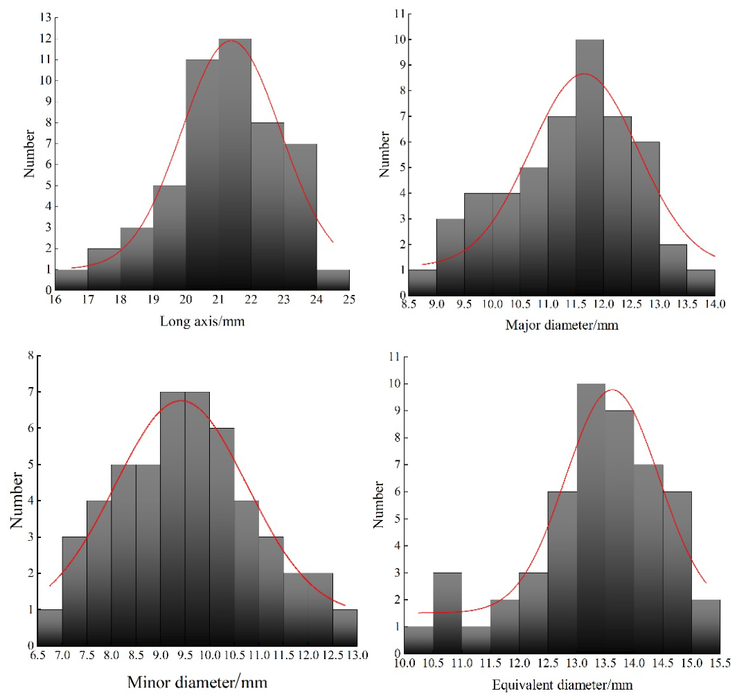
The frequency distributions of fruit dimensions were then analyzed, and the results, shown in Figure 2, followed an approximately normal distribution. The average mass of a single goji berry was 1.25 g, as measured using a high-precision electronic balance (CN-LQC20002, Youliweite, Kunshan, China). The particle density, determined using the Archimedes water-displacement method [14], was 840.47 kg/m³.

$$\left\{\begin{array}{l}\phi ={\displaystyle \frac{\sqrt[3]{D_{\mathrm{x}}{D}_{\mathrm{y}}{D}_{\mathrm{z}}}}{D_{\mathrm{x}}}}\times 100\%\\ D_{\mathrm{p}}=\sqrt[3]{D_{\mathrm{x}}{D}_{\mathrm{y}}{D}_{\mathrm{z}}}\end{array}\right.$$

(1)

where φ is fruit sphericity (%), D_p is the equivalent diameter (mm), and D_x, D_y, and D_z are the long axis, major diameter, and minor diameter, respectively.

2.2. Determination of Intrinsic Parameters of Goji Berries

(1)

Elastic modulus

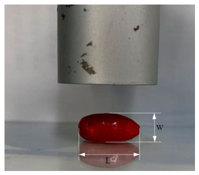
Compression tests were performed on fresh goji berries using an SMS texture analyzer [15]. The compression procedure is illustrated in Figure 3. The intrinsic parameters, including shear modulus, elastic modulus, and Poisson’s ratio, were determined [16]. A compressive load was applied in the W direction until the maximum critical deformation was reached. The compression test was conducted using a P/45 probe (45 mm diameter cylindrical aluminum probe, Stable Micro Systems Ltd., Godalming, Surrey, UK) at a constant loading rate of 1 mm/s. The probe displacement was controlled during the compression process to ensure gradual and stable contact with the fruit surface. Six individual goji berries were selected for compression testing, and the force–deformation responses were recorded for elastic modulus calculation. The loading force and deformation were recorded, and the elastic modulus of fresh goji berries was calculated using Equation (2).

$$E={\displaystyle \frac{F/S}{(W_1-W_2)/W_1}}$$

(2)

where E is the elastic modulus of fresh goji berries (Pa), F is the loading force when the sample reaches the critical elastic deformation state (N), and S is the cross-sectional area of the sample, approximated as an elliptical area (m²).

(2)

Poisson’s ratio

The texture analyzer was used to compress the fruit in the W direction to the maximum critical deformation, while the deformations in both the L and W directions were measured synchronously with a vernier caliper. Poisson’s ratio was then calculated using Equation (3).

$$\nu ={\displaystyle \frac{\left|{\epsilon }_2\right|}{\left|{\epsilon }_1\right|}}={\displaystyle \frac{(L_2-L_1)/L_1}{(W_2-W_1)/W_1}}$$

(3)

where $\nu$ is the Poisson’s ratio of fresh goji berries, ${\epsilon }_1$ is the strain in the loading direction, ${\epsilon }_2$ is the axial strain, L₁ and L₂ are the original and compressed sample lengths (mm), respectively, and W₁ and W₂ are the original and compressed sample widths (mm), respectively.

(3)

Shear modulus

The shear modulus of the goji berry fruit was calculated using Equation (4).

$$G={\displaystyle \frac{E}{2(1+\nu )}}$$

(4)

where G is the shear modulus of fresh goji berries (Pa).

2.3. Physical Piling Experiment

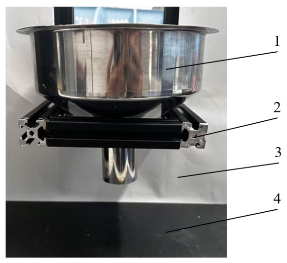
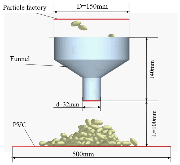
Physical piling experiments were conducted using the funnel method [17,18]. The funnel used in the experiment had an inlet diameter D = 150 mm and an outlet diameter d = 32 mm, and the vertical distance L between the outlet and the receiving plate was 100 mm. The experimental setup is shown in Figure 4.

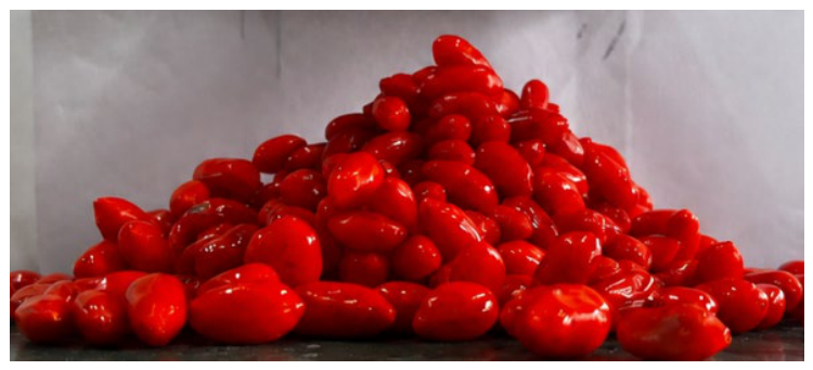
The experimental procedure was as follows: Five hundred fresh goji berries of uniform size were slowly and uniformly introduced through the funnel inlet. The piling experiment was repeated 10 times under the same experimental conditions. The AoR and Height obtained from each experiment were recorded. The mean values were used as the macroscopic response targets for DEM calibration. The variability of the experimental measurements was characterized using standard deviation (SD). After passing through the outlet, the particles accumulated on the receiving plate to form a pile, as shown in Figure 5.

The AoR and Height of the goji berry pile were measured. The Height was measured by placing a horizontal plate on the top surface of the particle pile after stabilization. A right-angle ruler was used to measure the vertical distance between the base plane and the horizontal plate, and this distance was taken as the Height. The ruler resolution was 1 mm. Because the pile boundary was approximately linear, the boundary slope was obtained by linear fitting, and the AoR was calculated as the arctangent of the fitted slope [19].

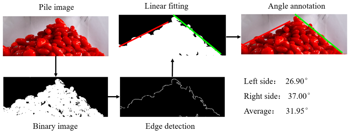
During image acquisition, the particle pile was photographed from the side view using a digital camera (EX-Z2000, CASIO COMPUTER CO., LTD., Tokyo, Japan) under the same experimental conditions. The camera was positioned perpendicular to the observation plane to minimize perspective distortion, and the original image resolution was 4032 × 3024 pixels. The obtained images were processed using MATLAB R2024a (MathWorks, Natick, MA, USA). The pile images were converted into grayscale images and binarized to separate the particle pile from the background. Edge detection was subsequently performed to extract the pile boundary, and the boundary profile was used for linear fitting. The arctangent of the fitted line slope was taken as the AoR. The angles of the left and right slopes were calculated separately, and the final AoR was determined as the average value of the two fitted slopes. The processing workflow is shown in Figure 6.

3. Calibration of Microscopic Parameters

3.1. DEM Model Construction and Parameter Setting

This section defines the key contact parameters to be calibrated and their ranges, and establishes the DEM simulation model of goji berry for parameter calibration. These steps provide the data basis for subsequent experimental design and parameter optimization.

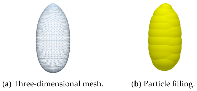
Based on the three-axis dimensions and ellipsoidal morphological characteristics of goji berry particles obtained from physical measurements, a three-dimensional goji berry particle model was established, as shown in Figure 7a. The model was imported into EDEM 2022 (Altair Engineering Inc., Troy, MI, USA) in .stl format for particle filling. The filling result is shown in Figure 7b, forming the goji berry particle model used for simulation. The STL-based particle model was directly used to represent the irregular geometry of fresh goji berries without multi-sphere approximation. The same particle geometry was applied to all simulated particles, while the experimentally measured size variation was not directly introduced into the DEM simulation.

According to the dimensions of the physical accumulation-test device, a virtual test bench consisting of a funnel, support, and PVC receiving plate was established, as shown in Figure 8. In the DEM simulation, 500 goji berry particles were generated using the particle factory, corresponding to the number used in the physical accumulation experiment. The particle generation rate was set to 30 particles/s, and the particles were generated above the funnel inlet with an initial velocity of zero. Under gravitational acceleration (9.81 m/s²), the particles deposited naturally to form the accumulation structure. The funnel inlet diameter, outlet diameter, and vertical distance from the outlet to the receiving plate in the simulation model were kept consistent with those in the physical experiment, so that the virtual accumulation process could reproduce the experimental conditions as closely as possible.

DEM is a time-driven numerical simulation method based on a soft-sphere model, and it uses contact laws to simulate interactions between particles [20]. In this study, the surfaces of goji berry particles were considered dry during the accumulation experiments, and no additional liquid adhesion between particles was introduced. Therefore, interparticle adhesion forces were not considered during the simulation. The Hertz-Mindlin (no-slip) contact model was used to describe the contact interactions between goji berries and PVC [21]. Although fresh goji berries are soft and deformable biological particles, the objective of this study was to calibrate effective DEM parameters for reproducing their macroscopic accumulation behavior rather than to fully describe their internal viscoelastic deformation characteristics. The influence of moisture-dependent adhesion and viscoelastic effects was not explicitly considered, which represents a limitation of the present simplified DEM representation.

According to the input requirements of EDEM simulations, the coefficient of restitution (e), static friction coefficient (μ_s), and rolling friction coefficient (μ_r) for goji berry-goji berry and goji berry-PVC contacts were selected as the parameters to be calibrated, giving a total of six microscopic contact parameters. The Poisson’s ratio, density, and shear modulus of goji berries were measured by physical experiments, whereas the material parameters of PVC were determined from the literature [22]. The fixed time step was set to 2.9256 × 10⁻⁵ s, which was approximately 28.2% of the Rayleigh time step (1.036 × 10⁻⁴ s). The total simulation duration was 18 s, and simulation data were saved at intervals of 0.01 s. The simulations were performed using the CPU solver with 8 parallel processing cores. The specific DEM parameters and their value ranges are listed in

Table 2. DEM sampling parameter ranges.

DEM Parameter	Symbol	Value/Range
Poisson’s ratio of goji berry	ν_p	0.32
Density of goji berry	ρ_p	840.47 (kg/m3)
Shear modulus of goji berry	G_p	4.3 × 104 (Pa)
Poisson’s ratio of PVC	ν_w	0.4
Density of PVC	ρ_w	1300 (kg/m3)
Shear modulus of PVC	G_w	1.12 × 109 (Pa)
Coefficient of restitution (goji-goji)	e_gg	0.1–0.4
Static friction coefficient (goji-goji)	μs_gg	0.35–0.75
Rolling friction coefficient (goji-goji)	μr_gg	0.02–0.07
Coefficient of restitution (goji-PVC)	e_gp	0.2–0.5
Static friction coefficient (goji-PVC)	μs_gp	0.4–0.8
Rolling friction coefficient (goji-PVC)	μr_gp	0.1–0.3

.

3.2. Calibration Procedure

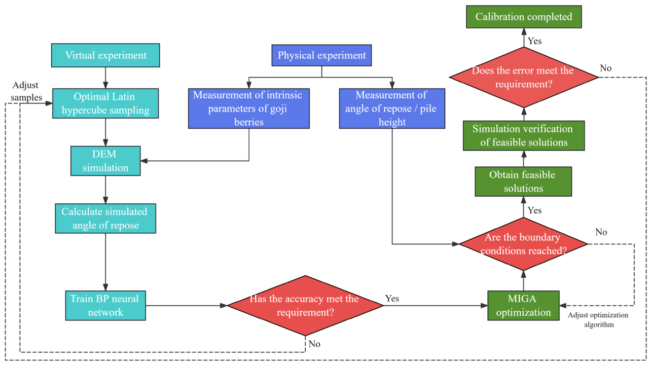
This section describes the design-of-experiments (DoE) strategy used for goji berry parameter calibration. The proposed method systematically combines a BP neural network [23] with optimal Latin hypercube sampling (OLHS) [24] and the multi-island genetic algorithm (MIGA) [25] to complete the calibration task.

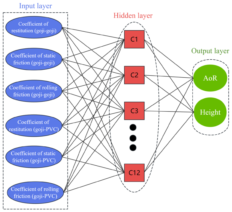
First, virtual experimental sample points were generated using OLHS, and EDEM 2022 was used to obtain the corresponding response values through simulation. The BP neural network was trained using the generated dataset. The network consisted of six input neurons corresponding to the six microscopic contact parameters and two output neurons representing AoR and Height. A single hidden layer containing 12 neurons was adopted. The input and output variables were normalized to the range of 0.1–0.9 using the mapminmax method. The hidden layer used the tansig activation function, while the output layer used the purelin activation function. The Bayesian regularization back-propagation algorithm (trainbr) was employed for training, with a maximum of 1500 epochs and a training goal of 1 × 10⁻⁴ based on mean squared error. Finally, measured experimental data were incorporated, and MIGA was used to optimize the surrogate model, enabling efficient calibration of the goji berry DEM model. The overall workflow is shown in Figure 9.

3.2.1. Virtual Experimental Design

Common experimental design methods for DEM simulations include central composite design, full factorial design, Latin hypercube sampling (LHS), and optimal Latin hypercube sampling (OLHS) [24]. The first two methods are widely used in conventional experimental design, whereas the latter two are less frequently adopted.

Although LHS ensures uniform marginal distributions through stratified sampling, its random pairing mechanism can produce uneven distributions in the multidimensional sample space [26]. OLHS optimizes variable pairing by introducing the maximin distance criterion, maximizing the minimum distance between sample points and thereby providing better space-filling characteristics for constructing DEM datasets with a limited number of samples [27,28]. Considering the high computational cost of DEM simulations, OLHS was adopted in this study to obtain reliable and uniformly distributed simulation data with a limited number of samples, thereby establishing a robust foundation for subsequent parameter calibration.

The OLHS design was implemented as follows [29]:

• Sampling scale and range. Six microscopic parameters were calibrated. Each variable x_i (i = 1, 2, …, 6) was assigned a range [x_i^l, x_i^u]. The number of sampling points was set to 150.
• Equal-probability stratification. The value range of each variable x_i was divided into 150 continuous subintervals of equal probability: x_i^l = x_i⁰ < x_i¹ < … < x_i^j < … < x_i¹⁴⁹ = x_i^u, ensuring that each subinterval had the same probability of being sampled.
• Within-stratum random sampling. One sample value was randomly and independently selected from each subinterval, generating 6 × 150 independent sample values in total.
• Optimized pairing. The random pairing used in standard LHS was optimized. First, the sample values of variables x₁ and x₂ were paired randomly without repetition to form 150 two-dimensional points. The points were then sequentially extended to six dimensions by adding the sample values of x₃, x₄, …, x₆. During this process, the pairing scheme was searched and adjusted according to the maximin distance criterion. The objective function was max(min(d_ij)), where d_ij was calculated using the Euclidean distance (Equation (5)). In this study, the OLHS procedure was implemented using MATLAB’s lhsdesign function with the maximin criterion and 20 iterations for optimizing the sampling distribution. A total of 150 samples were generated for six microscopic contact parameters to construct the DEM simulation dataset. Iterations was used to obtain the most uniform and dispersed sample distribution in the design space.

$$\mathrm{d}(x_i,x_j)=d_{ij}={\left[{\displaystyle \sum _n^m\left|x_i^k-x_j^k\right|}\right]}^{1/2}$$

(5)

6.

Generation of the sampling matrix. A 6 × 150 sampling matrix was finally obtained. Each row corresponded to one design variable, and each column represented one microscopic-parameter combination for virtual DEM experiments.

3.2.2. Approximate Modeling Based on a BP Neural Network

A BP neural network is a multilayer feedforward network trained using the error back-propagation algorithm. Its principle involves calculating outputs through forward propagation and updating network weights and biases through error back-propagation to minimize the difference between predicted and target outputs [30,31]. The network typically consists of an input layer, one or more hidden layers, and an output layer, with full connections between adjacent layers and no connections within the same layer [32]. Its working principle is shown in Figure 10.

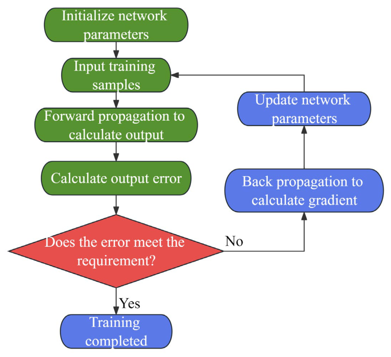
The BP neural network computation consists of three key steps: forward propagation, error calculation, and back propagation [33]. The overall training process is shown in Figure 11.

(1) Forward propagation. The six microscopic parameters were transmitted from the input layer to the output layer through the hidden layer. Each neuron performed weighted summation followed by activation function transformation (Equations (6)–(8)).

$${\mathrm{z}}_{\mathrm{j}}={\displaystyle \sum _{\mathrm{i}=1}^{\mathrm{n}}{W}_{\mathrm{ih}}^{\mathrm{ji}}}{\mathrm{x}}_{\mathrm{i}}+{\mathrm{b}}_{\mathrm{h}}^{\mathrm{j}}$$

(6)

where W_ih^ji is the weight from the ith input-layer neuron to the jth hidden-layer neuron, and b_hj is the bias of the jth hidden-layer neuron.

$${\mathrm{a}}_{\mathrm{j}}=\mathrm{f}({\mathrm{z}}_{\mathrm{j}})$$

(7)

The input O_k of the kth output-layer neuron was calculated as the weighted sum of hidden-layer outputs plus the bias (Equation (8)). The final output y_k was likewise processed through an activation function.

$${\mathrm{O}}_{\mathrm{k}}={\displaystyle \sum _{\mathrm{j}=1}^{\mathrm{n}}{W}_{\mathrm{ho}}^{\mathrm{kj}}}{\mathrm{a}}_{\mathrm{j}}+{\mathrm{b}}_{\mathrm{o}}^{\mathrm{k}}$$

(8)

(2) Error calculation. The mean squared error (MSE) was used to calculate the total error E between the network-predicted output and the target output (Equation (9)).

$$E={\displaystyle \frac{1}{2}}{{\displaystyle \sum _{\mathrm{k}=1}^{\mathrm{m}}({\mathrm{d}}_{\mathrm{k}}-{\mathrm{y}}_{\mathrm{k}})}}^2$$

(9)

where E is the total error, d_k is the kth target output, and y_k is the kth output predicted by the neural network.

(3) Back propagation. The chain rule was used to calculate the gradients of the error with respect to each weight and bias. All weights and bias parameters were then updated in the negative gradient direction (Equation (10)), progressively reducing the total error E.

$$\left\{\begin{array}{l}{\omega }_1\leftarrow {\omega }_0-\eta {\displaystyle \frac{\partial E}{\partial {\omega }_0}}\\ {\mathrm{b}}_1\leftarrow {\mathrm{b}}_0-\eta {\displaystyle \frac{\partial E}{\partial {\mathrm{b}}_0}}\end{array}\right.$$

(10)

where the $\frac{\partial E}{\partial \omega }$ and $\frac{\partial E}{\partial b}$ to the weight and bias represent the corresponding gradients, the ω₁ and b₁ terms represent the new weight and bias, and η is the learning rate.

In the calibration process, OLHS was first used to construct the variable matrix of parameters to be calibrated and to generate simulation sample points with good space-filling properties. The DEM simulation results at each sample point were then used as training data for the BP neural network, allowing an approximate model from microscopic parameters to macroscopic responses to be established. On this basis, MIGA was used to conduct a global search over the input space of the surrogate model and obtain the optimal parameter solution set. Finally, the representative solution set was verified through EDEM simulations, and the calibrated parameters were determined.

3.3. Parameter Calibration Based on MIGA

Compared with conventional single-population genetic algorithms, the MIGA global search algorithm introduces multiple subpopulations with periodic migration, which provides a mechanism for maintaining population diversity during optimization [34].

3.3.1. MIGA

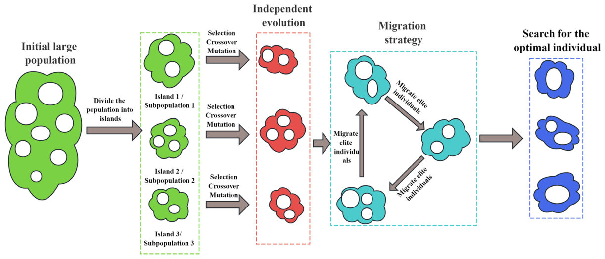
MIGA divides the population into multiple subpopulations, or islands. A conventional genetic algorithm is executed independently on each island, and selected individuals are exchanged periodically among islands according to a migration strategy. This mechanism of distributed evolution with periodic migration effectively balances local exploitation and global exploration, mitigates premature convergence, and provides an optimization mechanism for maintaining population diversity in complex multimodal problems [35]. The optimization process is illustrated in Figure 12.

In the optimization scheme, MIGA was configured with 5 islands and 40 individuals per island. The initial populations were randomly generated within the normalized parameter range of [−1, 1]. Tournament selection (size = 3), arithmetic crossover, and mutation (probability = 0.05, amplitude coefficient = 0.1) were employed during evolution. The best individual of each island was retained and migrated cyclically among islands every 10 generations. The optimization was terminated after 870 iterations, where each iteration consisted of 10 generations of island evolution followed by migration. A random seed of 2026 was fixed using the MATLAB twister generator to ensure reproducibility.

3.3.2. Constraints and Objective Function

In this study, the AoR and Height were selected as key response variables and predicted using the BP neural network. The optimization objective was to minimize the deviation between the predicted values and the centers of the target response intervals. The target response intervals and input-variable ranges were imposed as constraints during the feasible-solution search [36]. The mathematical formulation is given in Equations (11) and (12):

Objective function and constraints:

$$\left\{\begin{array}{l}\min F(x)={\displaystyle \frac{\left|Ao{R}_{pred}(x)-Ao{R}_{tar}\right|}{Ao{R}_{high}-Ao{R}_{low}}}+{\displaystyle \frac{\left|Heigh{t}_{pred}(x)-Heigh{t}_{tar}\right|}{Heigh{t}_{high}-Heigh{t}_{low}}}\\ s.t.\left\{\begin{array}{l}31\le Ao{R}_{pred}(x)\le 34\\ 64\le Heigh{t}_{pred}(x)\le 69\\ x_{i,\min }\le x_i\le x_{i,\max }(i=1,2,\mathrm{3...6})\end{array}\right.\end{array}\right.$$

(11)

where

$$\left\{\begin{array}{l}Ao{R}_{tar}={\displaystyle \frac{Ao{R}_{low}+Ao{R}_{high}}{2}}\\ Heigh{t}_{tar}={\displaystyle \frac{Heigh{t}_{low}+Heigh{t}_{high}}{2}}\end{array}\right.$$

(12)

where x_i denotes the six microscopic parameters to be calibrated; x_i,min and x_i,max are the lower and upper bounds of each parameter, respectively; the AoR_pred, Height_pred are the predicted values; and AoR_tar, Height_tar the centers of the target intervals.

The optimization objective was therefore to identify an effective set of DEM microscopic parameters that could reproduce the experimentally observed macroscopic responses of goji berries.

4. Results and Discussion

4.1. Neural-Network Accuracy and Feasible-Solution Analysis

4.1.1. Prediction Accuracy of the BP Neural Network

OLHS was used to generate 150 sample sets, each consisting of the six microscopic parameters to be calibrated. EDEM simulations were then performed for each parameter set, and the AoR and Height were measured. After excluding samples that failed to form stable pile structures, 137 valid datasets were obtained. In this study, an invalid pile was defined as a simulation case in which particles could not reach a stable accumulation state within the simulation period, resulting in the inability to obtain reliable Height and AoR values. The excluded cases corresponded to parameter combinations that produced unrealistic accumulation behavior under the investigated parameter ranges rather than random removal of simulation results.

These data were randomly divided into training, validation, and test sets at a ratio of 70%, 15%, and 15%, respectively. A fixed random seed (2026) with the Twister algorithm was adopted during dataset partitioning to ensure reproducibility. For the 137 valid datasets, 95, 20, and 22 samples were assigned to the training, validation, and test sets, respectively. The detailed training dataset used for BP neural network development is provided in Supplementary Table S1.

To evaluate the predictive performance of the BP neural network for AoR and Height, the coefficient of determination (R², Equation (13)) and root mean square error (RMSE) were used for quantitative assessment [37]. An R² value closer to 1 indicates a stronger linear correlation between predicted and actual values, whereas a smaller RMSE indicates lower overall prediction error and higher fitting accuracy.

$$R^2=1-{\displaystyle \frac{{{\displaystyle \sum _{\mathrm{t}=1}^{\mathrm{m}}(y_{\mathrm{t}}-{\stackrel{\wedge }{\mathrm{y}}}_{\mathrm{t}})}}^2}{{{\displaystyle \sum _{\mathrm{t}=1}^{\mathrm{m}}(y_{\mathrm{t}}-\stackrel{-}{\mathrm{y}})}}^2}}$$

(13)

where R² is the coefficient of determination, y_t is the simulated value of the tth sample, ŷ_t is the predicted value of the tth sample, ȳ is the mean of the true values, where m represents the number of samples in the corresponding dataset used for evaluation.

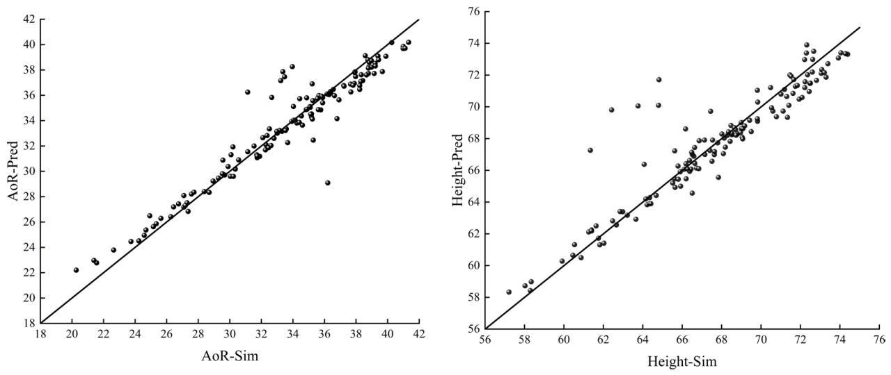
For the independent test dataset, the R² and RMSE values of AoR were 0.9415 and 1.0633, respectively, while those of Height were 0.9429 and 0.8447, respectively. Figure 13 shows the correlation between the simulated and predicted values. The scatter points for both responses are closely distributed around the y = x reference line, indicating good agreement between predicted and simulated values.

Although individual samples showed deviations, the overall error remained small, demonstrating that the BP neural network model achieved satisfactory prediction accuracy on the available datasets and could be used as a surrogate model for subsequent parameter optimization and feasible-solution screening.

4.1.2. Analysis of Feasible Solution Parameters

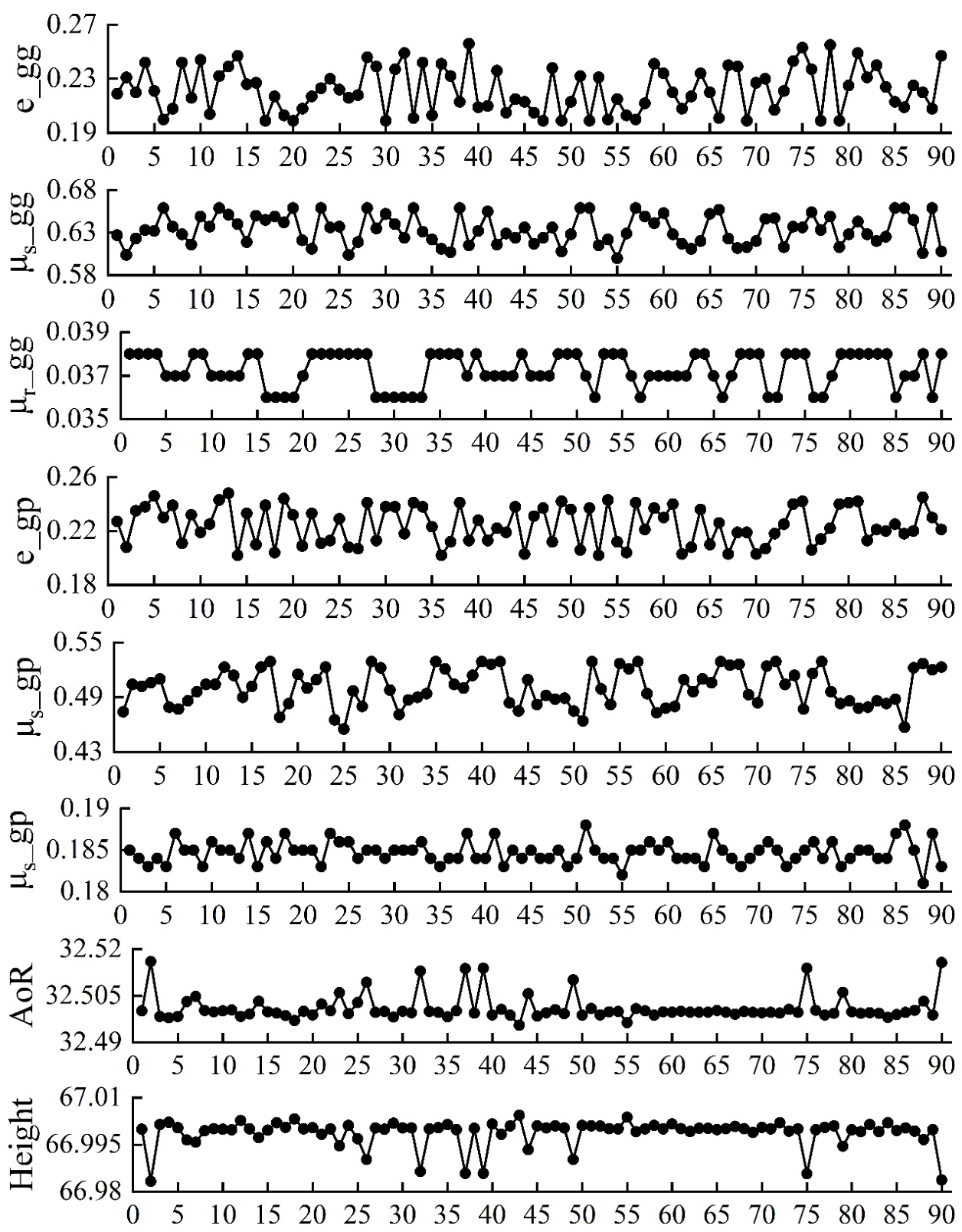
MIGA was used to perform an inverse search on the trained BP neural network model. Under the imposed constraints, 90 feasible solutions were obtained, indicating that multiple microscopic parameter combinations could reproduce similar macroscopic accumulation responses, and their parameter distributions are shown in Figure 14. The existence of multiple feasible solutions indicates that the inverse calibration problem has certain non-uniqueness. Therefore, the selected parameter combination should be regarded as an effective DEM parameter set for reproducing the macroscopic accumulation behavior of fresh goji berries rather than the unique intrinsic microscopic properties of the particles.

Figure 14 shows the distributions of feasible parameters obtained from the local concentrated search. Combined with the dispersion values in

Table 3. Distribution intervals of feasible solutions.

Variable	Calibration Interval	Dispersion (%)
e_gg	0.199–0.256	19.00
μs_gg	0.600–0.659	14.75
μr_gg	0.036–0.038	4.00
e_gp	0.202–0.248	15.33
μs_gp	0.455–0.529	18.50
μr_gp	0.181–0.188	3.50

, the results indicate that the parameters varied to different degrees. The dispersion values of μ_r_gg (4%) and μ_r_gp (3.5%) were low, indicating that these parameters were highly concentrated among feasible solutions and more strictly constrained during the calibration process. By contrast, e_gg (19%), μ_s_gg (14.75%), e_gp (15.33%), and μ_s_gp (18.5%) showed moderate dispersion, indicating relatively wider feasible intervals within the calibrated solution set.

For the output responses, the fluctuations in AoR and Height were very small, with values concentrated within 32.4955–32.52° and 66.98–67.01 mm, respectively. This indicates that although some input parameters exhibited dispersion, synergistic interactions among parameters allowed the AoR and Height to remain stably near the target intervals.

Overall, the feasible-solution distribution simultaneously reflected parameter diversity and response stability: the input parameters varied to different extents, whereas the macroscopic responses remained highly concentrated. This demonstrates the effectiveness of the local concentrated search strategy and the ability of the BP neural network to precisely control target responses, providing diverse and reliable candidate parameter combinations for DEM calibration.

4.2. Evaluation of Optimized DEM Parameters Through Numerical Simulation and Physical Experiments

4.2.1. Numerical Simulation Evaluation of Optimized Parameters

To verify the rationality and stability of the feasible solutions, representative parameter combinations were selected from the feasible-solution set for DEM simulation evaluation. The solution with the minimum total deviation was selected as the final parameter set for subsequent DEM and Dynamic experimental evaluation. In addition, four representative feasible solutions (Solutions 22, 15, 56, and 84) were selected from the feasible-solution set to evaluate the consistency between BP neural network predictions and DEM simulation results. One additional feasible solution (Solution 2) was selected to further verify whether the parameter constraints could still be satisfied under a relatively different parameter combination.

As shown in

Table 4. Verification results of feasible solutions.

Solution No.		22	15	56	84	2
e_gg μs_gg μr_gg e_gp μs_gp μr_gp		0.217	0.226	0.203	0.224	0.231
		0.611	0.619	0.629	0.625	0.604
		0.038	0.038	0.037	0.038	0.038
		0.233	0.233	0.204	0.220	0.208
		0.509	0.502	0.521	0.483	0.504
		0.183	0.183	0.185	0.184	0.184
Response	AoR-Pred Height-Pred	32.5001 67.0000	32.4998 66.9996	32.5008 66.9991	32.498 67.002	32.516 66.9833
	AoR-Sim Height-Sim	32.00 65.63	32.17 64.23	31.16 63.82	31.75 63.95	33.67 64.78
Error (%)	AoR Height	1.56	1.02	4.30	2.36	3.43
		2.09	4.31	4.98	4.77	3.40

, the errors between the BP-neural-network predictions and DEM simulation values were all within 5%, indicating that the predictions were generally consistent with the simulations and confirming both the validity of the feasible solutions and the accuracy of the model. Among all feasible solutions, the parameter combination with the minimum total deviation was identified as the representative solution. The corresponding parameters were e_gg = 0.203, μ_s_gg = 0.642, μ_r_gg = 0.037, e_gp = 0.244, μ_s_gp = 0.483, and μ_r_gp = 0.185, corresponding to AoR = 32.5 and Height = 67.00. This parameter set was subsequently used for DEM simulation and Dynamic experimental evaluation.

4.2.2. Dynamic Experimental Evaluation of Optimized Parameters

To further evaluate the applicability of the optimized DEM parameters under different particle motion conditions, a cylindrical rolling experiment was conducted to assess the rearrangement and slip behavior of goji berries under dynamic rotational conditions. Unlike the funnel piling test used for DEM parameter calibration, the cylindrical rolling test introduces a different particle-flow configuration, in which particles undergo continuous rearrangement and redistribution under rotational disturbance. This experiment was therefore performed to further examine the capability of the optimized parameters in describing the dynamic behavior of goji berries.

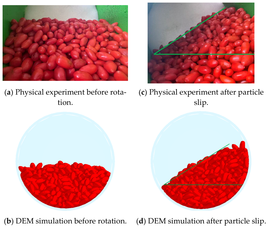
The physical experiment was conducted using a PVC cylindrical container with an outer diameter of 200 mm, a length of 340 mm, and a wall thickness of 5 mm. A total of 900 fresh goji berries were placed inside the cylinder. The cylinder was rotated at a constant angular velocity of 0.0873 rad/s (approximately 5°/s). When apparent particle slip occurred during rotation, the rotation was stopped, and the particle motion state and final stacking configuration were recorded. Figure 15a,c show the initial particle arrangement before rotation and the particle state after slip, respectively.

A corresponding DEM model was established according to the experimental procedure. In the simulation, 900 goji berry particles were generated at a rate of 500 particles/s, and the particle generation process lasted for 2 s. Subsequently, the particles were allowed to stabilize for 2.6 s to eliminate disturbances caused by the initial particle generation process. The cylindrical container was then rotated at a constant angular velocity of 0.0873 rad/s, consistent with the physical experiment. The total simulation time was set to 10 s to reproduce the particle motion and slip behavior during the rotational process. Figure 15b,d present the corresponding DEM results before rotation and after particle slip, respectively.

Figure 15 compares the physical experiment and DEM simulation results during the cylindrical rolling process. It can be observed that the DEM simulation successfully reproduced the overall particle movement trend, rearrangement process, and post-slip stacking configuration of goji berries under rotational motion. The particle-flow regions and slip characteristics observed in the physical experiment showed good agreement with those obtained from DEM simulation, indicating that the optimized DEM parameters can not only describe the static accumulation behavior but also capture the dynamic response characteristics of goji berries under rotational disturbance.

It should be noted that this experiment was conducted to evaluate the applicability of the optimized DEM parameters under different particle motion conditions rather than to replace the original calibration process. Future studies involving independent validation using different batches of goji berries or alternative loading configurations are expected to further assess the generalizability of the calibrated DEM parameters.

4.2.3. Discussion and Comparison with Previous Studies

Previous studies have also calibrated DEM parameters for fresh goji berries. Reference [11] determined the contact parameters through physical experiments combined with DEM simulations and response surface optimization, providing reliable parameters for reproducing the macroscopic stacking behavior of goji berries. In comparison, this study developed an integrated calibration framework based on OLHS, BP neural network, and MIGA, which can establish the nonlinear relationship between microscopic parameters and macroscopic responses and reduce repeated DEM simulations during optimization. Although the calibrated parameters differ from those reported in Reference [11], such differences are reasonable because DEM parameters are effective parameters influenced by particle representation, contact models, and calibration objectives. The proposed method achieved satisfactory prediction accuracy (R² > 0.94 for both responses) and provides an efficient strategy for DEM parameter calibration of irregular agricultural particles.

4.3. Limitations of the Proposed Calibration Framework

Although the proposed OLHS-BP-MIGA framework achieved satisfactory calibration performance for fresh goji berries, several limitations should be acknowledged. First, this study focused on establishing an integrated calibration framework rather than developing a new optimization algorithm. Therefore, direct quantitative comparisons with other calibration strategies, such as conventional Latin hypercube sampling (LHS)-based methods or response surface methodology (RSM), were not conducted. These comparisons require additional independent DEM simulations with different sampling and optimization schemes, which would substantially increase computational costs.

Second, the contribution of each individual component (OLHS, BP neural network, and MIGA) was not separately quantified in the current study. Future work will perform systematic benchmark and ablation studies to further investigate the influence of sampling strategies, surrogate models, and optimization algorithms on DEM parameter calibration accuracy.

5. Conclusions

To address the difficulty of directly measuring microscopic contact parameters in DEM simulations of goji berries, this study proposed an integrated calibration framework combining optimal Latin hypercube sampling (OLHS), a BP neural network, and a multi-island genetic algorithm (MIGA). Using fresh ‘Ningqi No. 7’ goji berries as the research object, physical experiments, virtual simulations, and optimization algorithms were integrated to obtain reliable calibration results. The main conclusions are as follows:

• Physical characterization of fresh goji berry particles and construction of the DEM calibration dataset were completed. The measured particle density, shear modulus, and Poisson’s ratio of goji berries were 840.47 kg/m³, 4.3 × 10⁴ Pa, and 0.32, respectively. The particle sphericity was less than 0.8, indicating an overall ellipsoidal shape. Physical accumulation experiments produced an average AoR of 32.87 ± 2.20° and an average Height of 65.57 ± 4.10 mm, providing macroscopic response benchmarks for DEM parameter calibration. On this basis, OLHS was used to generate a 6 × 150 microscopic-parameter sample matrix. Virtual simulations were conducted for the coefficients of restitution, static friction coefficients, and rolling friction coefficients in goji berry-goji berry and goji berry-PVC contacts, thereby constructing the microscopic-macroscopic response dataset for BP neural network training and MIGA optimization.
• A microscopic contact-parameter prediction and optimization calibration method based on the BP neural network and MIGA was established. The BP neural network surrogate model accurately described the nonlinear relationship between microscopic contact parameters and macroscopic accumulation responses. For the AoR and Height, the R² values of the test set reached 0.9415 and 0.9429, respectively, and the RMSE values were 1.0633 and 0.8447, respectively, indicating satisfactory prediction performance on the available dataset. On this basis, MIGA was used to globally optimize the surrogate model, and 90 feasible solutions were obtained after 870 iterations. When the optimized representative microscopic parameters were input into EDEM simulation, the relative errors of the AoR and Height were all less than 5%, verifying the effectiveness and reliability of the combined OLHS-BP-MIGA calibration method.
• Multi-level validation by BP neural network prediction, EDEM simulation, and physical accumulation experiments demonstrated the reliability of the optimal contact-parameter combination. The relative errors between BP predictions and EDEM simulation values for representative feasible solutions were all less than 5%, indicating that the established surrogate model could effectively characterize the mapping relationship between microscopic contact parameters and macroscopic accumulation responses. Further DEM simulation using the optimal parameter combination showed that the simulated AoR and Height were highly consistent with the physical experimental results, with errors of 0.76% and 1.33%, respectively. This demonstrates that the parameter combination can reliably reproduce the actual accumulation behavior of fresh goji berry particles and can provide a reliable parameter basis for DEM simulation analysis of postharvest goji berry processing equipment.

In summary, the proposed OLHS-BP-MIGA integrated calibration framework provides an effective strategy for calibrating DEM microscopic contact parameters of fresh goji berries. By combining optimal sampling, nonlinear surrogate modeling, and evolutionary optimization, this framework can reduce the dependence on direct trial-and-error calibration and establish the relationship between microscopic contact parameters and macroscopic piling responses. The calibrated parameters provide a reliable basis for DEM simulation analysis and structural optimization of postharvest goji berry processing equipment.

In practical agricultural applications, the calibrated DEM parameters can be directly applied to virtual testing and optimization of postharvest processing equipment, such as conveying, sorting, and packaging systems. These applications can help predict particle flow behavior, evaluate collision-related damage risks, and improve equipment design efficiency. Therefore, the proposed framework provides a practical solution for accelerating DEM-based agricultural equipment development beyond laboratory-scale parameter calibration.

However, the present study has some limitations. The calibrated DEM parameters were obtained based on fresh ‘Ningqi No. 7’ goji berries under specific experimental conditions, and their applicability to other cultivars, moisture conditions, and loading scenarios requires further investigation.

References

1. Mansouri, M.; El Youssoufi, M.S.; Nicot, F. Numerical simulation of the quicksand phenomenon by a 3D coupled discrete element–lattice Boltzmann hydromechanical model. Int. J. Numer. Anal. Methods Geomech. 2017, 41, 338–358. [Google Scholar] [CrossRef] [Scilit]
2. Moncada, M.; Toledo, P.; Betancourt, F.; Rodríguez, C.G. Torque analysis of a gyratory crusher with the discrete element method. Minerals 2021, 11, 878. [Google Scholar] [CrossRef] [Scilit]
3. Feng, Y.; Yuan, Z. Discrete element method modeling of granular flow characteristics transition in mixed flow. Comput. Part. Mech. 2020, 8, 21–34. [Google Scholar] [CrossRef] [Scilit]
4. Wiącek, J.; Stasiak, M.; Kafashan, J. Structural and micromechanical properties of ternary granular packings: Effect of particle size ratio and number fraction of particle size classes. Materials 2020, 13, 339. [Google Scholar] [CrossRef] [Scilit]
5. Pasha, M.; Hare, C.; Ghadiri, M.; Gunadi, A.; Piccione, P.M. Effect of particle shape on flow in discrete element method simulation of a rotary batch seed coater. Powder Technol. 2016, 296, 29–36. [Google Scholar] [CrossRef] [Scilit]
6. Liu, X.Y.; Wang, Q.W.; Wang, Y.W.; Dong, Q.X. Review of calibration strategies for discrete element model in quasi-static elastic deformation. Sci. Rep. 2023, 13, 13264. [Google Scholar] [CrossRef] [Scilit]
7. Irazábal, J.; Salazar, F.; Vicente, D.J. A methodology for calibrating parameters in discrete element models based on machine learning surrogates. Comput. Part. Mech. 2023, 10, 1031–1047. [Google Scholar] [CrossRef] [Scilit]
8. He, P.; Fan, Y.W.; Pan, B.L.; Zhu, Y.F.; Liu, J.; Zhu, D.R. Calibration and verification of dynamic particle flow parameters by the back-propagation neural network based on the genetic algorithm: Recycled polyurethane powder. Materials 2019, 12, 3350. [Google Scholar] [CrossRef] [Scilit]
9. Do, H.Q.; Aragón, A.M.; Schott, D.L. A calibration framework for discrete element model parameters using genetic algorithms. Adv. Powder Technol. 2018, 29, 1393–1403. [Google Scholar] [CrossRef] [Scilit]
10. Zhou, H.; Li, K.T.; Qin, Z.Y.; Wang, S.S.; Wang, X.Z.; Sun, F.Y. Discrete element model of oil peony seeds and the calibration of its parameters. Agriculture 2024, 14, 1092. [Google Scholar] [CrossRef] [Scilit]
11. Yang, Y.; Ren, S.M.; Li, J.; Chang, J.Q.; Yu, S.; Sun, C.; Chen, T.M. Calibration and testing of discrete element modeling parameters for fresh goji berries. Appl. Sci. 2022, 12, 11629. [Google Scholar] [CrossRef] [Scilit]
12. Zhu, Y.; Zhu, L.C.; Guo, W.K.; Han, Z.H.; Wang, R.X.; Zhang, W.P.; Yuan, Y.W.; Gao, J.B.; Liu, S.C. Multiscale static compressive damage characteristics of kiwifruit based on the finite element method. Foods 2024, 13, 785. [Google Scholar] [CrossRef] [Scilit]
13. Li, T.; Shu, J.; Wu, Y.; Li, Y.; Wu, B.; Deng, Z.; Huang, J.; Galindo, R.; Molina Gómez, F. Influence of particle rotation on the shear characteristics of calcareous-sand and silica-bead granular materials. Materials 2024, 17, 5827. [Google Scholar] [CrossRef] [Scilit]
14. Ma, C.; Liu, F.; Ran, L.; Mi, J.; Lu, L.; Wang, S.; Ge, X.; Jin, B.; Zhang, L.; Yan, Y. Assessment of phenotypic characteristics, polysaccharide composition, and hypoglycemic potential in different commercial grades of Lycium barbarum: A comprehensive study using HPLC and NMR. Foods 2025, 14, 3862. [Google Scholar] [CrossRef] [Scilit]
15. Du, J.; Ni, Z.J.; Wang, W.; Thakur, K.; Ma, R.H.; Ma, W.P.; Wei, Z.J. Carbon dot-mediated photodynamic treatment improves the quality attributes of post-harvest goji berries (Lycium barbarum L.) via regulating the antioxidant system. Foods 2024, 13, 955. [Google Scholar] [CrossRef] [Scilit]
16. Ben, Z.Y.; Zhang, X.B.; Yang, D.X.; Chen, K.J. An experimental and numerical study for discrete element model parameters calibration: Gluten pellets. Agriculture 2023, 13, 744. [Google Scholar] [CrossRef] [Scilit]
17. Liu, F.; Li, D.P.; Zhang, T.; Lin, Z. Analysis and calibration of quinoa grain parameters used in a discrete element method based on the repose angle of the particle heap. INMATEH-Agric. Eng. 2020, 61, 77–86. [Google Scholar] [CrossRef] [Scilit]
18. Peng, Y.; Zhang, S.; Wan, J.; Yang, Y.; Tao, K.; Ma, L.; Yang, G.; Yang, L.; Wang, M. Numerical study of granular flow in a slit funnel with a novel structure to avoid particle clogging. PLoS ONE 2023, 18, e0286591. [Google Scholar] [CrossRef] [Scilit]
19. Li, P.L.; Ucgul, M.; Lee, S.H.; Saunders, C. A new approach for the automatic measurement of the angle of repose of granular materials with maximal least square using digital image processing. Comput. Electron. Agric. 2020, 172, 105356. [Google Scholar] [CrossRef] [Scilit]
20. Rackl, M.; Hanley, K.J. A methodical calibration procedure for discrete element models. Powder Technol. 2017, 307, 73–83. [Google Scholar] [CrossRef] [Scilit]
21. Dun, G.; Sheng, Q.; Ji, X.; Li, H.; Ma, C.; Li, X.; Sun, H.; Wang, L.; Ma, C.; Yu, Z.; et al. Parameter optimization of the notched blade spiral fertilizer discharger for pineapple orchards based on DEM. Front. Mech. Eng. 2025, 11, 1535013. [Google Scholar] [CrossRef] [Scilit]
22. Wu, J.X.; Shen, Y.H.; Yang, S.D.; Feng, Z.P. Simulation of track-soft soil interactions using a discrete element method. Appl. Sci. 2022, 12, 2524. [Google Scholar] [CrossRef] [Scilit]
23. Ma, X.J.; Guo, M.J.; Tong, X.; Hou, Z.F.; Liu, H.Y.; Ren, H.Y. Calibration of small-grain seed parameters based on a BP neural network: A case study with red clover seeds. Agronomy 2023, 13, 2670. [Google Scholar] [CrossRef] [Scilit]
24. Li, X.K.; Xing, W.B.; Jiang, Q.L.; Chen, Z.Z.; Zhao, W.B.; Xu, Y.P.; Cao, Y.; Ming, W.Y.; Ma, J. RBF-based integrated optimization method of structural and turning parameters for low-floor axle bridge. Metals 2024, 14, 273. [Google Scholar] [CrossRef] [Scilit]
25. Lan, Y.Z.; Zhao, Y.; Zhai, Z.P.; Fan, M.H.; Li, F.S. Numerical simulation and optimization of the gas-solid coupled flow field and discharging performance of straw crushers. Fluid Dyn. Mater. Process. 2024, 20, 2565–2583. [Google Scholar] [CrossRef] [Scilit]
26. Palar, P.S.; Saves, P.; Robani, M.D.; Verstaevel, N.; Garouani, M.; Aligon, J.; Shimoyama, K.; Morlier, J.; Gaudou, B. Interpretable and explainable surrogate modeling for simulations: A state-of-the-art survey and perspectives on explainable AI for decision-making. Arch. Comput. Methods Eng. 2026, 33, 1–55. [Google Scholar] [CrossRef] [Scilit]
27. Zhang, M.; Jiao, J.; Zhang, J.; Zhang, Z.J. High-efficiency data fusion aerodynamic performance modeling method for high-altitude propellers. Drones 2024, 8, 229. [Google Scholar] [CrossRef] [Scilit]
28. Wu, H.; Tan, H.B.; Xu, Z.L.; Li, Y.Z. Multi-objective optimization of variable density multi-layer insulation for liquid hydrogen containers based on reduced-order surrogate model. Processes 2023, 11, 1383. [Google Scholar] [CrossRef] [Scilit]
29. Xia, X.; Li, W.; Li, P. A new class of asymptotic maximin distance Latin hypercube designs. Can. J. Stat. 2025, 53, e11836. [Google Scholar] [CrossRef] [Scilit]
30. Zhang, J.X.; Qu, S.R. Optimization of backpropagation neural network under the adaptive genetic algorithm. Complexity 2021, 2021, 1718234. [Google Scholar] [CrossRef] [Scilit]
31. Diao, H.W.; Zeng, F.D.; Liu, Y.Z.; Dou, M.L.; Zhang, Z.C.; Zhao, Z.H. Research on the calibration of discrete elemental parameters of yam bean based on GA-BP improved neural network algorithm. Processes 2025, 13, 1537. [Google Scholar] [CrossRef] [Scilit]
32. Zeng, F.D.; Liu, L.M.; Liu, Y.Z.; Bai, H.B.; Li, C.X.; Zhao, Z.H. Experimental study on DEM parameters calibration for organic fertilizer by the particle swarm optimization−backpropagation neural networks. Sci. Rep. 2025, 15, 25629. [Google Scholar] [CrossRef] [Scilit]
33. Liu, Z.Y.; Yuan, J.M.; Shen, J.H.; Hu, Y.; Chen, S.L. A new DEM calibration method for wet and stick materials based on the BP neural network. Powder Technol. 2024, 448, 120228. [Google Scholar] [CrossRef] [Scilit]
34. Song, X.F.; Dai, F.; Zhang, F.W.; Wang, D.M.; Liu, Y.C. Calibration of DEM models for fertilizer particles based on numerical simulations and granular experiments. Comput. Electron. Agric. 2023, 204, 107507. [Google Scholar] [CrossRef] [Scilit]
35. Harada, T.; Alba, E.; Luque, G. A fresh approach to evaluate performance in distributed parallel genetic algorithms. Appl. Soft Comput. 2022, 119, 108540. [Google Scholar] [CrossRef] [Scilit]
36. Wei, Z.; Zhou, C.P.; Zhang, F.; Zhou, C.C. Reliability Optimization of the Honeycomb Sandwich Structure Based on A Neural Network Surrogate Model. Materials 2023, 16, 7465. [Google Scholar] [CrossRef] [Scilit]
37. Cheng, K.J.; Yan, J.X.; Li, G.; Ma, W.W.; Guo, Z.C.; Wang, W.N.; Li, H.L.; Da, Q.H.; Li, X.H.; Yao, Y.D. Remote sensing inversion of nitrogen content in silage maize plants based on feature selection. Front. Plant Sci. 2025, 16, 1554842. [Google Scholar] [CrossRef] [Scilit]
Figure 1. Schematic diagram of the three principal dimensions of a goji berry fruit.
Agriculture 16 02012 g001
Figure 2. Geometric characteristics of goji berries.
Agriculture 16 02012 g002
Figure 3. Schematic diagram of goji berry compression.
Agriculture 16 02012 g003
Figure 4. Physical piling experimental setup: 1. funnel; 2. support; 3. background board; 4. base plate.
Agriculture 16 02012 g004
Figure 5. Physical pile of goji berries.
Agriculture 16 02012 g005
Figure 6. Workflow for AoR calculation.The red and green lines represent the linear fitting lines of the left and right sides of the particle pile boundary, respectively.
Agriculture 16 02012 g006
Figure 7. Simulation model of a goji berry particle.
Agriculture 16 02012 g007
Figure 8. Virtual simulation test apparatus.The upper, middle, and lower red lines represent the boundaries of the particle factory, funnel outlet, and PVC plate, respectively.
Agriculture 16 02012 g008
Figure 9. Parameter calibration workflow.The cyan, blue, green, and red boxes represent the virtual experiment process, physical experiment process, optimization and verification process, and decision nodes, respectively.
Agriculture 16 02012 g009
Figure 10. Structure of the BP neural network model used for DEM parameter calibration.The blue, red, and green nodes represent the input layer, hidden layer, and output layer, respectively.
Agriculture 16 02012 g010
Figure 11. Flowchart of the BP neural network training algorithm.The green, blue, and red boxes represent the forward propagation process, back propagation and parameter update process, and error decision node, respectively.
Agriculture 16 02012 g011
Figure 12. Schematic diagram of the MIGA optimization process.The green, red, cyan, and blue regions represent the population initialization and island division stage, independent evolution stage, migration strategy stage, and optimal-individual search stage, respectively.The dashed boxes indicate the corresponding stages and subpopulations involved in the MIGA optimization process.
Agriculture 16 02012 g012
Figure 13. Comparison of simulated and predicted values for AoR and Height based on all 137 samples.
Agriculture 16 02012 g013
Figure 14. Parameter and response distributions of feasible solutions.
Agriculture 16 02012 g014
Figure 15. Comparison between physical experiment and DEM simulation during cylindrical rolling test. The green lines indicate the fitted boundary lines of the particle pile after particle slip.
Agriculture 16 02012 g015