Non-Destructive Classification of Apple Watercore Severity Levels Using Near-Infrared Hyperspectral Imaging

Abstract

Apple watercore is an internal physiological disorder that affects fruit quality and storage stability. This study developed a non-destructive approach for classifying watercore severity in 737 Aksu ‘Fuji’ apples using near-infrared hyperspectral imaging (930–1720 nm). Watercore severity was quantified using the watercore severity index (WSI) derived from Fiji-based segmentation of equatorial cross-sectional images, and samples were classified into sound, slight, moderate, and severe classes according to published criteria. After spectral preprocessing, support vector machine (SVM), random forest (RF), baseline one-dimensional convolutional neural network (1D-CNN), and attention-enhanced 1D-CNN-CBAM-SE models were evaluated using five repeated stratified holdout experiments. SVM and 1D-CNN-CBAM-SE achieved comparable performance, with SVM obtaining an accuracy of 98.74% and a Macro-F1 score of 98.86%, and 1D-CNN-CBAM-SE achieving the same accuracy and a Macro-F1 score of 98.85%. Ablation experiments showed that attention modules improved the baseline 1D-CNN, with CBAM providing the major performance gain and the addition of SE further reducing performance variability across repeated experiments. Misclassifications were largely confined to adjacent severity classes. These results support the feasibility of NIR-HSI combined with spectral classification models for non-destructive watercore severity grading.

1. Introduction

Watercore is a common internal physiological disorder of apple fruit, characterized by water-soaked and translucent flesh tissue. In cultivars such as ‘Fuji’, moderate watercore is often associated with greater perceived sweetness and distinctive sensory attributes and is an important quality basis of ‘sugar-heart’ apples [1]. From a physiological perspective, watercore development is closely associated with sorbitol metabolism, changes in intercellular spaces, water transport, water-potential gradients, and sugar translocation [2,3,4,5]. However, when watercore becomes severe, affected tissues exhibit reduced gas diffusion capacity and increased susceptibility to internal disorders during storage, which may compromise fruit quality and commercial value [6,7]. Rapid, objective, and non-destructive classification of watercore severity in Aksu ‘sugar-heart’ apples from southern Xinjiang is therefore important for postharvest sorting, storage-risk assessment, and quality control.

At present, apple watercore is still detected mainly by empirical visual judgment, destructive cutting, or limited sampling. Although equatorial cutting and cross-sectional observation directly reveal the affected tissue, the procedure is destructive, inefficient, wasteful, and susceptible to subjective error, making it unsuitable for large-scale postharvest sorting or online inspection. Because watercore develops primarily inside the fruit, external phenotypic traits such as peel color and fruit shape cannot accurately indicate its presence or severity. Non-destructive methods based on spectral or imaging information are therefore needed for severity classification.

In recent years, optical non-destructive techniques, including visible/near-infrared (Vis/NIR) spectroscopy, near-infrared transmittance spectroscopy, and hyperspectral imaging, have been used to detect apple watercore and evaluate internal quality. Guo et al. [8] quantitatively assessed watercore severity and soluble solids content using near-infrared transmittance spectroscopy, demonstrating the feasibility of simultaneous evaluation of watercore and internal quality. Chang et al. [9] developed an online Vis/NIR spectroscopic system for sound-versus-watercore discrimination and reported prediction accuracies above 95%, with the best-performing model reaching 96%. Zhang et al. [10] combined Vis/NIR full-transmittance spectroscopy with analysis of variance to establish a dual-band ratio threshold model for online watercore detection. In subsequent work, Zhang et al. [11] investigated the effects of detection speed and fruit orientation; under an online detection speed of 0.5 m s⁻¹ and the optimal O3 orientation, a two-feature-wavelength LS-SVM model achieved success rates of 96.87% for watercored apples and 100% for healthy apples. Guo et al. [12] further applied hyperspectral interactance/transmittance imaging to discriminate watercore in Xinjiang-grown ‘Fuji’ apples. More recently, Wu et al. [13] developed a portable Vis/NIR system combined with 1DQCNN for four-level apple watercore grading and reported a test accuracy of 98.05%. Collectively, these studies demonstrate the progression of optical techniques from binary watercore detection toward quantitative multi-level severity grading.

Hyperspectral imaging simultaneously provides continuous spectral and spatial information and has considerable potential for non-destructive quality evaluation of agricultural products [14]. For internal-quality assessment of apples, Ma et al. [15] used near-infrared hyperspectral imaging to evaluate soluble solids content non-destructively; Fan et al. [16] combined spectral and textural features from hyperspectral reflectance images to improve soluble-solids prediction; and Lan et al. [17] used near-infrared hyperspectral imaging to characterize internal-quality heterogeneity in apple slices. In watercore detection, hyperspectral reflectance can capture changes in tissue water status, sugar-alcohol content, and light-scattering properties, providing a potential spectral basis for affected-area classification.

In addition to spectroscopic techniques, X-ray computed tomography (CT) and magnetic resonance imaging (MRI) have been used to detect apple watercore tissue. Herremans et al. [18] compared X-ray CT and MRI for watercore detection in several apple cultivars and found that both techniques could identify affected tissue, with MRI providing greater image contrast. Yu et al. [19] combined hyperspectral imaging and X-ray CT for non-destructive detection and three-dimensional structural analysis of different watercore grades, further demonstrating the value of imaging for tissue visualization and severity assessment. However, X-ray CT and MRI generally involve high equipment costs, complex operating conditions, and limited suitability for online implementation. Hyperspectral imaging is comparatively rapid, non-destructive, and information-rich and is therefore more suitable for studying watercore severity classification.

During hyperspectral modeling, spectral differences among watercore severity grades are often subtle, while raw spectra are susceptible to instrumental noise, baseline drift, surface-scattering effects, and variations in fruit shape. Direct modeling of raw spectra may therefore compromise model stability and generalizability. Conventional machine learning methods, such as support vector machines (SVMs) and random forests (RFs), are effective for classifying high-dimensional spectral data, whereas one-dimensional convolutional neural networks (1D-CNNs) can automatically learn local nonlinear relationships among adjacent wavelengths and have been applied to NIR and hyperspectral sequence modeling for agricultural-product classification [20,21]. The convolutional block attention module (CBAM) adaptively emphasizes informative features along the channel and spectral-position dimensions [22], whereas the squeeze-and-excitation (SE) module recalibrates channel responses to enhance discriminative features [23]. Attention-enhanced 1D-CNN architectures have also been applied to agricultural hyperspectral data, demonstrating their ability to emphasize informative spectral responses in complex classification tasks [24]. SE-enhanced one-dimensional networks using full-band hyperspectral inputs have likewise shown promising performance in agricultural-product classification [25]. Incorporating these attention mechanisms into a 1D-CNN may therefore enhance spectral feature representation and watercore severity classification performance.

Despite progress in binary watercore identification, online detection, and internal-quality prediction, three limitations remain. First, most studies distinguish watercored from healthy fruit but do not quantitatively grade the proportion of affected tissue. Second, relatively little work has addressed area-based watercore classification in the regionally distinctive ‘sugar-heart’ apples of Aksu using hyperspectral reflectance spectra. Third, because spectral differences among severity grades are subtle, accurate and robust classification remains challenging.

Accordingly, this study investigated commercially marketed Aksu ‘Fuji’ apples from southern Xinjiang. After hyperspectral image acquisition, a watercore severity index (WSI) was calculated from RGB images of equatorial cross-sections, and the samples were assigned to four classes: sound, slight, moderate, and severe. Following spectral preprocessing, conventional machine learning models (SVM and RF), a baseline 1D-CNN, and attention-enhanced 1D-CNN variants incorporating SE, CBAM, or their combination were developed and systematically compared. Ablation experiments were further conducted to quantify the individual and combined contributions of the attention modules to spectral feature learning and classification stability. The study therefore provides a framework for non-destructive four-level watercore severity assessment and evaluates the applicability of attention-enhanced spectral modeling for Aksu ‘sugar-heart’ apples.

2. Materials and Methods

2.1. Apple Samples

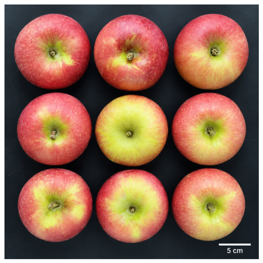
Commercially marketed Aksu ‘Fuji’ apples from southern Xinjiang were purchased in November 2025 from a local fruit and vegetable wholesale market in Alar, Xinjiang, China. Fruits with regular shape, relatively uniform size, similar maturity, and no visible mechanical damage, pest injury, decay, or other external defects were selected. After transport to the laboratory, the fruits were individually numbered, and malformed, damaged, or externally abnormal samples were excluded. A total of 737 valid samples were retained. Representative external appearances are shown in Figure 1.

To minimize the effect of temperature differences on near-infrared hyperspectral image acquisition and model performance, all samples were equilibrated for at least 24 h in a laboratory maintained at 20 °C and 60% relative humidity, allowing the fruit temperature to match the measurement environment. Before imaging, the fruit surfaces were gently wiped with a clean, soft cloth to remove dust and adhering material that could interfere with spectral reflectance. Hyperspectral images were then acquired sequentially for all samples, and sample identifiers and basic information were recorded.

2.2. Quantification of Watercore Area and Severity Grading

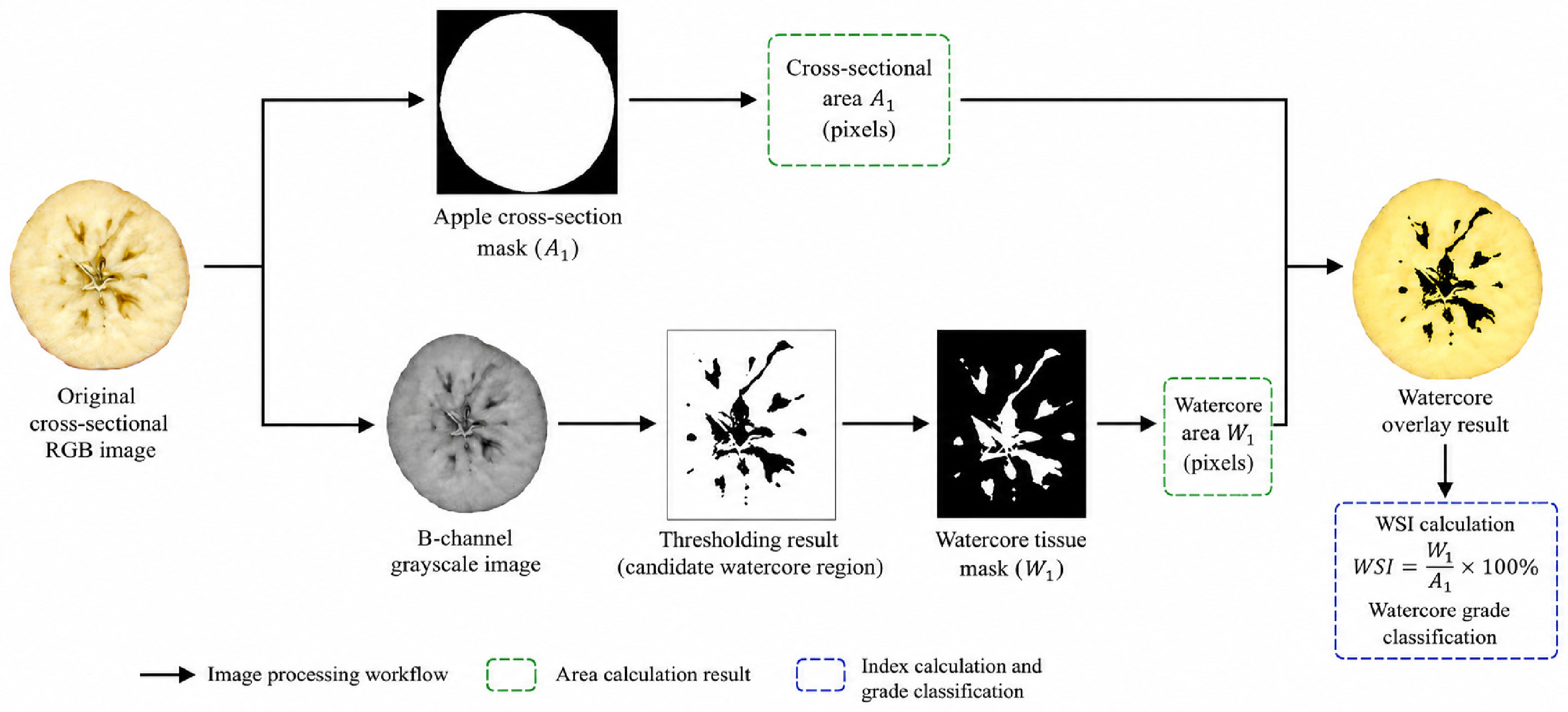
To quantify watercore severity, each apple was cut along the equatorial plane after hyperspectral imaging, and an RGB image of the cross-section was acquired using the rear camera of an Apple iPhone 16 Pro smartphone (Apple Inc., Cupertino, CA, USA) at a resolution of 3024 × 4032 pixels. The equatorial plane was selected as a standardized cross-section to ensure consistent two-dimensional quantification and comparison of watercore-affected area among fruits. The illumination conditions, camera-to-sample distance, imaging angle, background, and sample orientation were kept constant for all samples. The cross-sectional images were analyzed using a semi-automatic image-processing procedure in Fiji (ImageJ version 1.53t). The watercore-affected regions were identified based on their translucent appearance and color differences relative to the surrounding healthy tissues and were subsequently quantified to calculate the watercore severity index (WSI). The overall image-processing and WSI calculation workflow is shown in Figure 2.

First, the fruit contour was extracted according to the grayscale contrast between the apple cross-section and the background. Hole filling and morphological operations were applied to obtain a complete cross-sectional mask, and the number of pixels within the mask was recorded as A₁. The RGB image was then separated into individual channels. Because watercore tissue showed greater contrast from sound flesh in the B channel, a fixed grayscale threshold of 0–100 was applied to the 8-bit B-channel image to generate candidate watercore regions.

Connected-component filtering was subsequently performed, followed by limited manual correction to remove clearly identifiable non-watercore regions, including the core, seeds, peel-edge shadows, and other segmentation artifacts. All manual corrections were performed by a single operator according to predefined criteria and were restricted to the exclusion of these non-watercore regions; the watercore boundaries were not subjectively expanded or contracted. The same threshold, image-processing parameters, and correction criteria were applied to all 737 images. The final binary mask was regarded as the watercore region, and its pixel count was recorded as W₁.

The watercore severity index was calculated as

WSI = (W₁/A₁) × 100%

(1)

where W₁ is the number of pixels within the watercore-affected region and A₁ is the total number of pixels within the apple cross-sectional mask. Both W₁ and A₁ were quantified using Fiji.

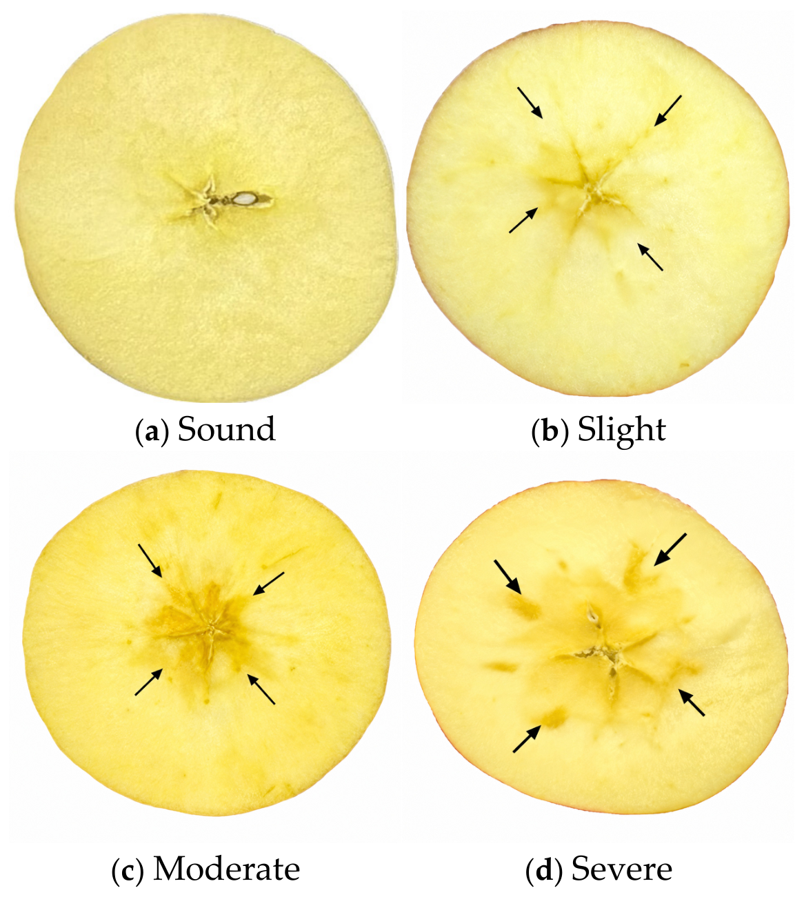
The severity thresholds were adopted from a previously published WSI-based grading scheme [26]. Based on the WSI values, the 737 apples were classified as sound (WSI < 1%), slight watercore (WSI 1–5%), moderate watercore (WSI 5–10%), or severe watercore (WSI > 10%). In the present study, these literature-derived thresholds were used as operational criteria for quantitative severity classification. The WSI-based approach directly quantified the proportion of watercore-affected tissue on the equatorial cross-section and was used to define the reference labels for subsequent spectral classification modeling. Independent expert-panel grading was not available in the present study. To examine the sensitivity of severity assignments to the literature-derived thresholds, a local threshold sensitivity analysis was performed. Each of the three WSI boundaries (1%, 5%, and 10%) was independently shifted by ±0.5 percentage points while the other two boundaries were held constant. For each perturbation, the number and proportion of samples whose severity labels changed relative to the original classification were recorded. In addition, the numbers of samples located within ±0.5 percentage points of each original grading boundary were determined. Representative equatorial cross-sectional images of the four severity classes are shown in Figure 3. The visible extent of translucent watercore-associated tissue generally increased with WSI-based severity grade.

To evaluate the intra-operator repeatability of the semi-automatic segmentation procedure, a stratified subset of 30 cross-sectional images covering all four severity classes was selected. The images were reprocessed in a separate session by the same operator using identical thresholding parameters and manual-correction criteria, without access to the initial segmentation results. Repeatability was evaluated using the mean absolute difference between the paired WSI measurements and the agreement rate of the resulting severity-class labels. Accordingly, this analysis was intended to evaluate procedural repeatability under consistent operating conditions. Independent validation against expert-annotated reference masks was beyond the scope of the present study and should be considered in future work.

2.3. Near-Infrared Hyperspectral Imaging System and Reflectance Acquisition

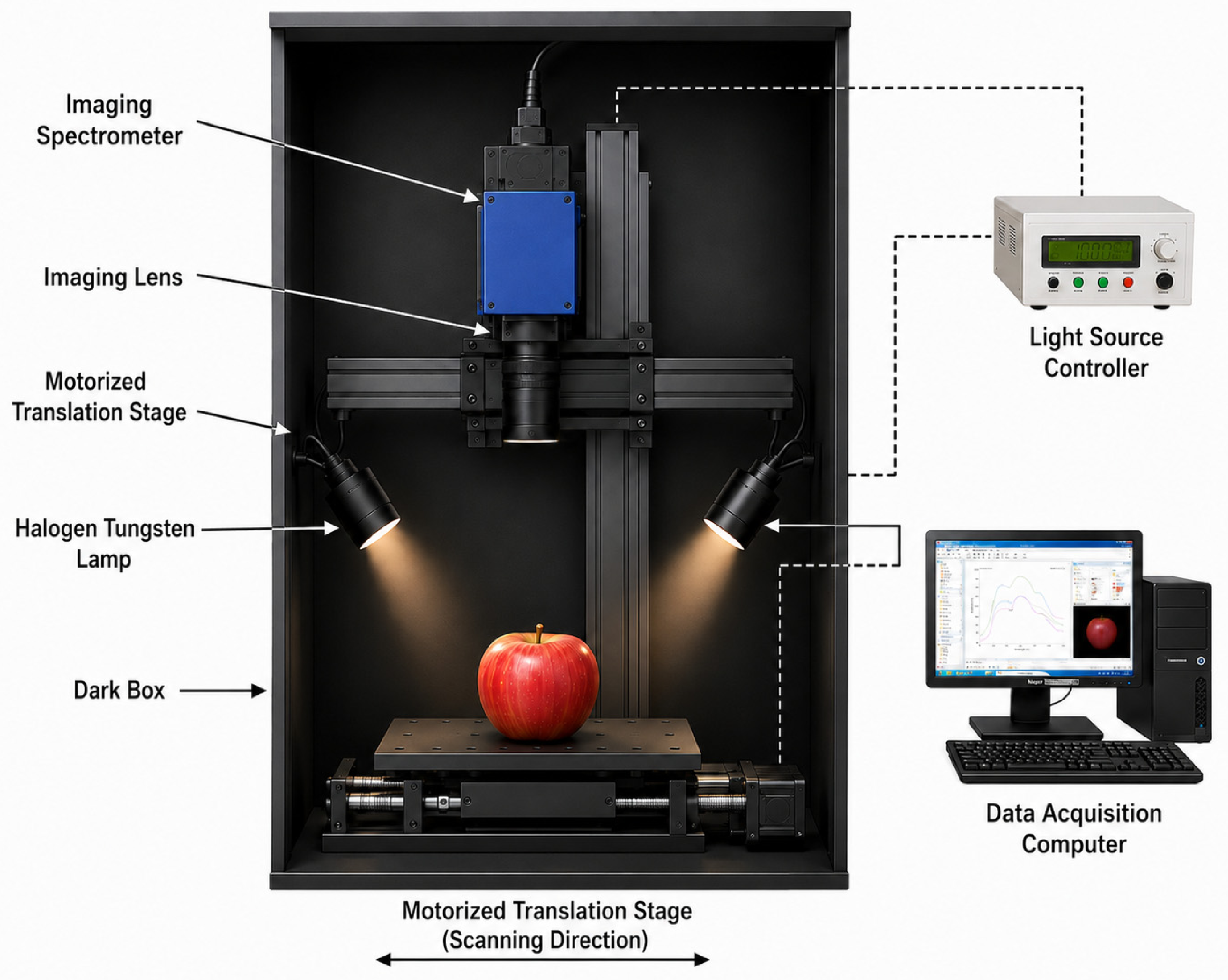
The near-infrared hyperspectral reflectance platform was a Solomon integrated hyperspectral imaging system (ISUZU OpticsCorp., Chupei, Hsinchu, Taiwan, China). The system comprised an imaging spectrometer, imaging lens, tungsten–halogen illumination, a motorized translation stage, a dark enclosure, a light-source controller, and a data-acquisition computer (Figure 4). Hyperspectral image acquisition was controlled using HSImager SW, whereas reflectance calibration, hyperspectral-image visualization, ROI extraction, and spectral export were performed using HSI Analyzer v1.0.

Hyperspectral images were acquired in reflectance mode over approximately 930–1720 nm, comprising 224 contiguous bands. Acquisition parameters, including exposure time, image gain, and translation-stage speed, were set through the acquisition software. Two tungsten–halogen lamps were positioned symmetrically on either side of the sample at 45° to the horizontal plane. The imaging lens was located above the sample at a vertical working distance of 30 cm, and the lamp power was 150 W. To minimize interference from ambient stray light, image acquisition was performed inside a dark enclosure. The system and lamps were warmed up for 15 min before acquisition to stabilize lamp output and detector response. Based on preliminary tests, the exposure time, image gain, and stage speed were set to 28 ms, 1, and 0.8 mm s⁻¹, respectively. Lamp position, working distance, fruit orientation, and camera settings were kept constant. Raw hyperspectral data were stored in RAW format, and wavelength information and acquisition parameters were recorded in the corresponding HDR files.

Hyperspectral Image Calibration and Spectral Extraction

Because raw hyperspectral images are affected by nonuniform illumination, detector dark current, and variation in system response, white- and dark-reference calibration was performed. The white reference was obtained by scanning a standard white diffuse-reflectance panel under the same acquisition conditions as the samples. The dark reference was acquired with the light sources switched off and the camera lens covered. Exposure time, scanning speed, and working distance were identical for the sample, white-reference, and dark-reference images.

The software supplied with the hyperspectral system was used for reflectance calibration. The calibrated relative-reflectance image was calculated as

R^c = (R^o − R^d)/(R^w − R^d)

(2)

where R^c is the calibrated relative-reflectance image, R^o is the raw hyperspectral image of the apple sample, R^w is the white-reference image, and R^d is the dark-reference image.

The calibrated hyperspectral images were imported into HSI Analyzer v1.0 for region-of-interest (ROI) extraction. The valid fruit region was delineated using the ROI tool provided by the software. Background pixels, edge-shadow regions, highlighted pixels, and isolated anomalous pixels were excluded according to consistent criteria applied to all samples. Reflectance values of all valid ROI pixels were averaged at each wavelength, yielding one representative mean spectrum containing 224 spectral variables for each apple.

2.4. Spectral Preprocessing

Raw near-infrared hyperspectral reflectance spectra are susceptible to random instrumental noise, baseline variation, and differences in surface scattering. To improve the signal-to-noise ratio and comparability among samples, the spectra were first smoothed using the Savitzky–Golay algorithm [27] with a window length of 7 and a second-order polynomial. Standard normal variate (SNV) transformation [28] was then applied to correct scattering effects. For each data split, standardization parameters were fitted using the training data only and subsequently applied to both the training and test sets, thereby preventing information leakage from the test set. After preprocessing, each apple was represented by 224 spectral bands for model development.

2.5. Model Inputs and Class Labels

The model input consisted of all 224 bands of the mean ROI reflectance spectrum for each apple. Sample identifiers were used only for traceability and were not included as predictors. The classification targets were the four severity classes determined from the Fiji-quantified WSI values using the published grading thresholds: sound, slight, moderate, and severe. No preselection based on partial least-squares regression coefficients or successive projections algorithm wavelengths was performed. Full-spectrum input was retained to preserve continuous wavelength information and to provide the convolutional and attention modules with a complete basis for automatically learning features associated with watercore severity.

2.6. Watercore Severity Classification Models

Four classifiers were developed to compare their ability to discriminate watercore severity: an SVM, an RF, a baseline 1D-CNN, and an attention-enhanced 1D-CNN-CBAM-SE. All models used the same 224 full-spectrum variables after Savitzky–Golay smoothing, SNV correction, and standardization, without additional wavelength selection. The outputs were the four severity classes: sound, slight, moderate, and severe.

2.6.1. Conventional Machine Learning Models

SVM and RF were used as conventional machine learning baselines. To ensure a fair comparison with CNN-based models, hyperparameter optimization was performed using the validation subset within each training split. For SVM, a radial basis function kernel was evaluated with combinations of C values (0.1, 1, 10, and 100) and γ values (0.001, 0.01, 0.1, 1, and scale). For RF, the number of trees (50, 100, and 200) and maximum tree depth (5, 10, 15, and None) were optimized. The optimal hyperparameters were selected according to validation Macro-F1 performance. The models were then re-trained using the combined training and validation subsets and evaluated on the independent test set. For reproducibility, each repeated experiment used the same random seed as the corresponding data split.

2.6.2. One-Dimensional Convolutional and Attention Models

The baseline 1D-CNN served as the deep learning reference model. Each preprocessed spectrum was represented as a single-channel sequence of length 224. The network consisted of three one-dimensional convolutional blocks with 64, 128, and 256 output channels and kernel sizes of 7, 5, and 3, respectively. All convolutional layers used a stride of 1 and padding sizes of 3, 2, and 1, respectively, thereby preserving the spectral-sequence length before pooling. Each convolutional layer was followed by batch normalization and rectified linear unit activation. Max pooling with a kernel size and stride of 2 was applied after the first two convolutional blocks, reducing the sequence length from 224 to 112 and subsequently to 56. Dropout with a rate of 0.4 was applied after each of the first two pooling layers. The output of the third convolutional block was processed using adaptive global average pooling, followed by dropout with a rate of 0.6 and a fully connected layer that produced four class logits corresponding to sound, slight, moderate, and severe watercore.

To construct the attention-enhanced networks, CBAM and/or SE modules were inserted after the batch-normalization and activation operations of each of the three convolutional blocks. In the combined 1D-CNN-CBAM-SE model, CBAM was applied first, followed by SE. The channel-attention branch of CBAM used both adaptive average pooling and adaptive max pooling to generate channel descriptors, which were processed by a shared multilayer perceptron with a reduction ratio of 8. The resulting channel-attention weights were generated using sigmoid activation. The spectral-position attention branch calculated the mean and maximum responses across channels, concatenated the two descriptors, and applied a one-dimensional convolution with a kernel size of 7 and padding of 3, followed by sigmoid activation. The SE module used adaptive global average pooling and two fully connected layers with a channel-reduction ratio of 8 to recalibrate the channel responses. Except for the attention modules, all networks used identical convolutional backbones, pooling operations, dropout settings, classification heads, and training parameters.

2.6.3. Model Training and Evaluation

Repeated stratified holdout experiments were performed using five fixed random seeds (42, 13, 29, 7, and 19). In each repetition, the samples were divided into a training set and a test set at a ratio of 7:3, yielding 515 training samples and 222 test samples. For the CNN-based models, 15% of the training set was further allocated as a validation subset for model selection and early stopping. The validation subset was also used for SVM and RF hyperparameter optimization to provide a consistent model-selection framework across algorithms. Spectral preprocessing and model development were performed in Python 3.11.9. The SVM and RF models were implemented using scikit-learn 1.8.0, whereas the CNN-based models were implemented using PyTorch 2.11.0 (CPU build, Meta Platforms, Inc., Menlo Park, CA, USA). The code was developed and executed in PyCharm 2024.3.6.1 (JetBrains, Prague, Czech Republic).

The CNN-based models were trained using class-weighted cross-entropy loss with a label-smoothing factor of 0.1 and the Adam optimizer, with an initial learning rate of 0.001, a batch size of 32, a weight decay of 5 × 10⁻⁴, and a maximum of 300 epochs. During training, online spectral augmentation was applied only to the training samples by adding Gaussian noise with a standard deviation of 0.005 and applying a random multiplicative scaling factor sampled uniformly from 0.9 to 1.1. No augmentation was applied to the validation or test samples. A cosine-annealing learning-rate scheduler was used throughout training. Early stopping was applied when the validation loss did not improve for 40 consecutive epochs, and the model parameters corresponding to the minimum validation loss were retained.

For the CNN-based models, spectral augmentation and label smoothing were used as model-specific regularization strategies. SVM and RF instead underwent validation-based hyperparameter optimization, while all models shared the same outer training–test splits, spectral preprocessing procedure, and test-set evaluation protocol. The comparison focused on the final predictive performance of each optimized model under its appropriate modeling framework.

Model performance was evaluated using accuracy and the Macro-F1 score. The means and standard deviations obtained from the five repetitions were used as the primary summary statistics. To examine class-specific errors, confusion matrices were generated by aggregating predictions from all five repeated stratified holdout experiments.

Because the repeated holdout splits shared samples across repetitions, the resulting performance estimates were not statistically independent. Consequently, no confirmatory hypothesis tests were conducted. Model comparisons were based primarily on mean performance, variability across repetitions, and the magnitude and consistency of the observed differences over the five repeated splits.

3. Results

3.1. Intra-Operator Repeatability of Watercore-Region Segmentation

For the 30 cross-sectional images processed twice, the mean absolute difference between the paired WSI measurements was 0.32 percentage points. The severity-class labels were identical for all 30 images, corresponding to a classification agreement rate of 100%. These results indicated good intra-operator repeatability of the semi-automatic segmentation procedure within the evaluated subset.

3.2. Sensitivity of WSI-Based Severity Classification to Grading Thresholds

Among the 737 apples, no sample was located within ±0.5 percentage points of the 1% WSI boundary, whereas 19 samples (2.58%) and 9 samples (1.22%) were located within ±0.5 percentage points of the 5% and 10% boundaries, respectively. When the 1% threshold was independently shifted to 0.5% or 1.5%, no sample changed severity class. Shifting the 5% threshold to 4.5% and 5.5% resulted in 7 (0.95%) and 12 (1.63%) samples changing class, respectively. Similarly, shifting the 10% threshold to 9.5% and 10.5% changed the classifications of 3 (0.41%) and 6 (0.81%) samples, respectively. Thus, under the ±0.5-percentage-point perturbation examined here, changes in severity assignment were limited to a small proportion of the dataset and occurred primarily around the 5% boundary.

3.3. Sample Distribution and Data Splitting

The final dataset contained 737 apples: 123 sound, 167 slight, 208 moderate, and 239 severe. Each of the five repetitions used stratified random sampling and a 7:3 training-to-test split. Because the class totals were fixed, every split contained 515 training samples and 222 test samples. The class distribution is presented in

Table 1. Distribution of apple samples by watercore severity class and stratified split.

Severity Class	Total	Training Set	Test Set
Sound	123	86	37
Slight	167	117	50
Moderate	208	145	63
Severe	239	167	72
Total	737	515	222

.

The training set contained 86 sound, 117 slight, 145 moderate, and 167 severe samples, while the corresponding test-set counts were 37, 50, 63, and 72. Class proportions in the training and test sets were therefore similar to those in the complete dataset. Although different samples were assigned to the training and test sets under the five random seeds, the number of samples in each class remained constant.

3.4. Spectral Characteristics of Apples with Different Watercore Severities

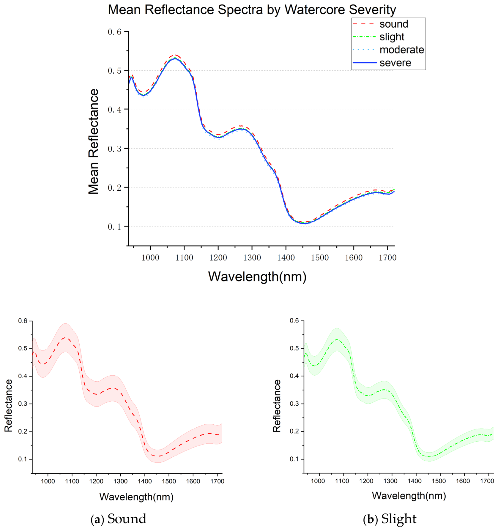
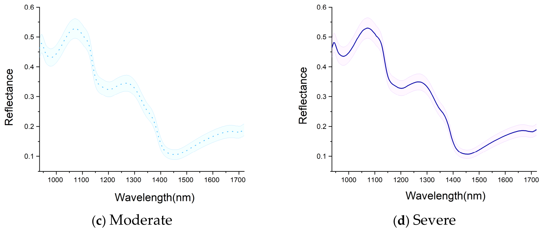
Figure 5 shows the mean hyperspectral reflectance curves of sound, slight, moderate, and severe apples over approximately 930–1720 nm. The four classes exhibited similar overall spectral trends, with pronounced features near 970 nm, 1200–1300 nm, and 1450 nm, indicating broadly comparable reflectance responses across severity levels.

Previous studies have reported that spectral features near 970, 1170, and 1450 nm in apples are primarily related to water absorption [29] and that absorption near 1450 nm in food systems is commonly associated with the first overtone of O–H stretching in water [30]. As shown in Figure 5, all severity classes exhibited similar peaks and troughs in these water-related regions, suggesting that changes in tissue water status may be an important contributor to the spectral response of watercored apples.

Across classes, sound apples generally exhibited slightly higher mean reflectance over most wavelengths, whereas the slight, moderate, and severe curves were closer together and crossed in several regions. Reflectance did not change monotonically with increasing affected area; rather, class differences were expressed as small local variations in amplitude. These findings indicate that individual wavelengths alone are unlikely to provide robust discrimination among severity classes, supporting the use of full-spectrum information and multivariate classification approaches.

Savitzky–Golay smoothing suppressed local high-frequency fluctuations while preserving the principal peak and trough positions. Subsequent SNV correction reduced baseline and amplitude differences caused by surface scattering and optical-path variation. The preprocessed spectra therefore provided normalized inputs for subsequent classification modeling.

3.5. Comparison of Classification Models

SVM, RF, baseline 1D-CNN, and 1D-CNN-CBAM-SE were compared as the four primary classification models using identical spectral preprocessing procedures and the same five stratified training–test splits. SVM and RF served as conventional machine learning baselines, the baseline 1D-CNN served as the deep learning reference model, and 1D-CNN-CBAM-SE represented the attention-enhanced architecture. Mean accuracy and Macro-F1 values with their standard deviations are reported in

Table 2. Performance of classification models for area-based watercore severity grading.

Model	Accuracy	Macro-F1
SVM	0.9874 ± 0.0077	0.9886 ± 0.0070
RF	0.9757 ± 0.0101	0.9772 ± 0.0092
Baseline 1D-CNN	0.9162 ± 0.0214	0.9255 ± 0.0178
1D-CNN-CBAM-SE	0.9874 ± 0.0053	0.9885 ± 0.0049

. The individual effects of SE and CBAM are examined separately in the ablation analysis in Section 3.6.

Values are means ± standard deviations over five repeated experiments.

The evaluated models showed different levels of performance in classifying watercore severity. Among the conventional machine learning approaches, SVM achieved a mean accuracy of 0.9874 ± 0.0077 and a Macro-F1 score of 0.9886 ± 0.0070, while RF achieved an accuracy of 0.9757 ± 0.0101 and a Macro-F1 score of 0.9772 ± 0.0092. These results show that both SVM and RF provided strong conventional baselines for full-spectrum NIR-HSI-based watercore severity classification, with SVM exhibiting higher mean performance than RF.

The baseline 1D-CNN achieved a mean accuracy of 0.9162 ± 0.0214 and a Macro-F1 score of 0.9255 ± 0.0178, showing lower performance and larger variability compared with the optimized conventional models. After incorporating attention mechanisms, the performance of CNN models improved substantially. The 1D-CNN-CBAM-SE model achieved a mean accuracy of 0.9874 ± 0.0053 and a Macro-F1 score of 0.9885 ± 0.0049, reaching comparable performance to SVM while showing lower variability across repeated experiments.

The improvement provided by the attention modules was further supported by the ablation analysis. Compared with the baseline 1D-CNN, the CBAM-SE model improved the Macro-F1 score from 0.9255 to 0.9885. Among the attention variants, CBAM provided the major contribution, whereas the addition of SE further reduced performance variability across repeated splits. Because the repeated holdout experiments shared samples across repetitions, the comparison was interpreted based on the magnitude and consistency of performance differences rather than confirmatory statistical testing.

3.6. Ablation Analysis of the Attention Architecture

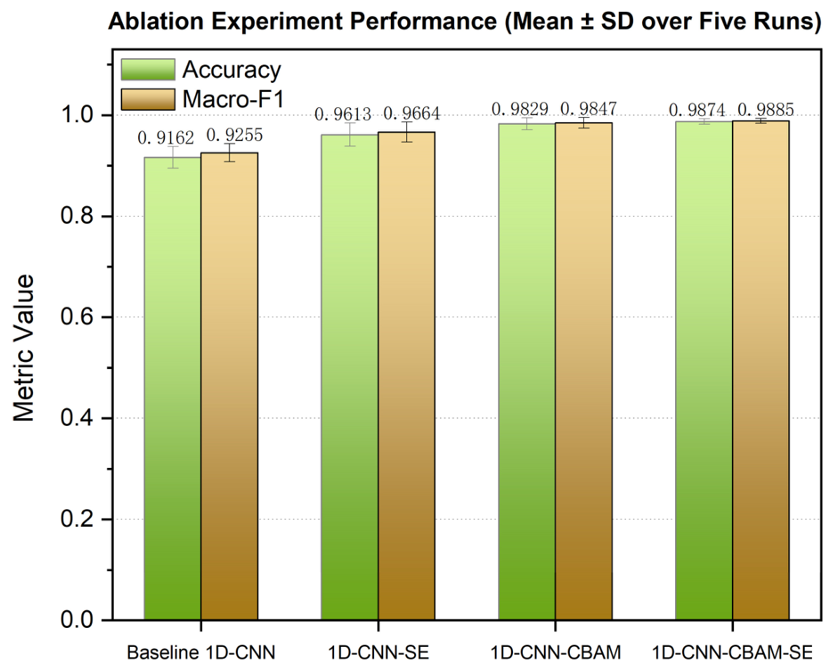
To examine the effects of SE, CBAM, and their combination on the baseline 1D-CNN, four networks were trained under identical backbone, preprocessing, split, and optimization settings. Their five-run accuracy and Macro-F1 results are summarized in

Table 3. Ablation results for different attention-module configurations.

Model	CBAM	SE	Accuracy (Mean ± SD)	Macro-F1 (Mean ± SD)
Baseline 1D-CNN	No	No	0.9162 ± 0.0214	0.9255 ± 0.0178
1D-CNN-SE	No	Yes	0.9613 ± 0.0229	0.9664 ± 0.0197
1D-CNN-CBAM	Yes	No	0.9829 ± 0.0119	0.9847 ± 0.0106
1D-CNN-CBAM-SE	Yes	Yes	0.9874 ± 0.0053	0.9885 ± 0.0049

and Figure 6.

Values are presented as means ± standard deviations over five repeated experiments. Because the repeated holdout splits partially overlapped, no confirmatory hypothesis tests were conducted.

The baseline 1D-CNN achieved a mean accuracy of 0.9162 ± 0.0214 and a mean Macro-F1 score of 0.9255 ± 0.0178. Incorporating SE alone improved the accuracy and Macro-F1 score to 0.9613 ± 0.0229 and 0.9664 ± 0.0197, respectively, indicating that channel-wise feature recalibration improved the representation capability of the baseline CNN.

Adding CBAM alone resulted in a larger performance improvement, increasing the mean accuracy and Macro-F1 score to 0.9829 ± 0.0119 and 0.9847 ± 0.0106, respectively. Compared with the baseline 1D-CNN, CBAM improved the Macro-F1 score by 5.92 percentage points and substantially reduced performance variability, suggesting that CBAM provided the major contribution to performance enhancement.

The combined 1D-CNN-CBAM-SE architecture achieved the highest mean performance among the four CNN architectures, with an accuracy of 0.9874 ± 0.0053 and a Macro-F1 score of 0.9885 ± 0.0049. Compared with 1D-CNN-CBAM, the combined architecture showed a further numerical increase of 0.45 percentage points in accuracy and 0.38 percentage points in Macro-F1. The corresponding standard deviations decreased from 0.0119 to 0.0053 for accuracy and from 0.0106 to 0.0049 for Macro-F1, indicating lower variability across the five repeated experiments.

Overall, the ablation results indicate that CBAM was the primary contributor to the improvement over the baseline 1D-CNN. The additional SE module provided further refinement and reduced performance variability across the repeated experiments.

3.7. Confusion Matrices and Error Analysis

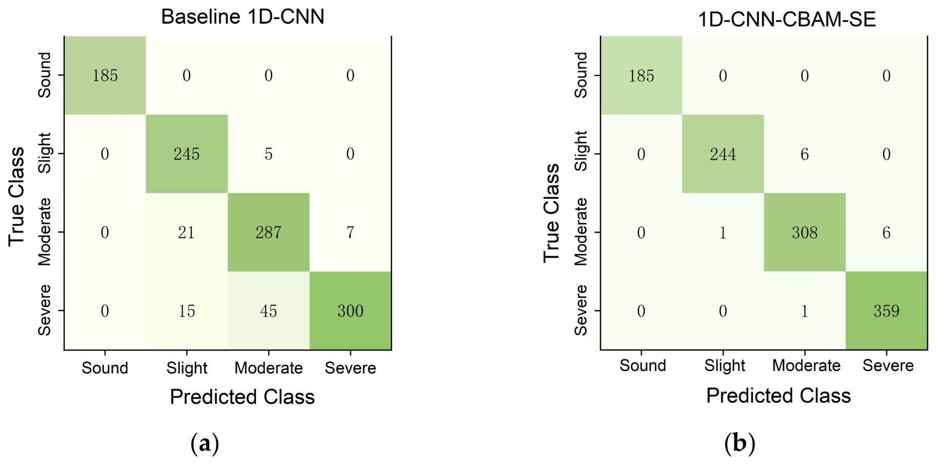
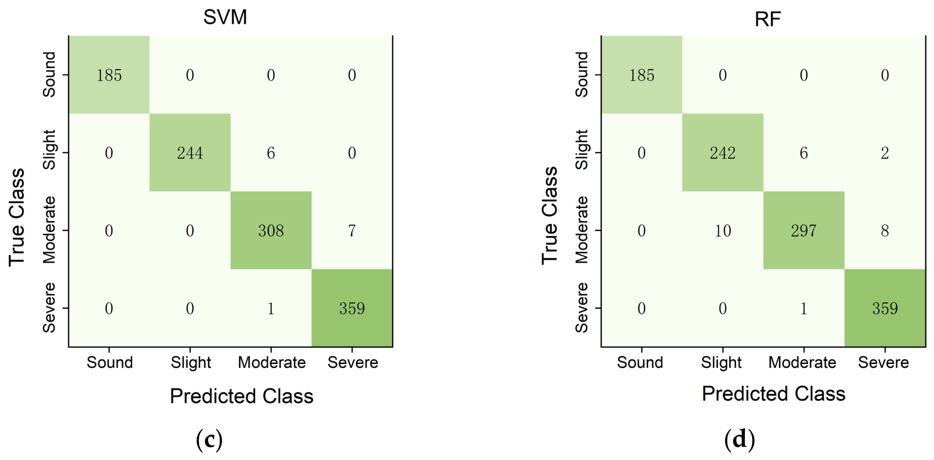
Confusion matrices were generated by aggregating test-set predictions across the five repeated stratified holdout experiments (Figure 7). A total of 1110 prediction instances were included in the aggregated analysis, comprising 185 sound, 250 slight, 315 moderate, and 360 severe samples across the five repetitions.

All four models correctly classified all sound cases in the aggregated analysis. The baseline 1D-CNN showed the greatest confusion among the severity classes, particularly for severe samples. Among severe samples, 45 were misclassified as moderate and 15 as slight. The 1D-CNN-CBAM-SE model substantially reduced these errors, with only 14 misclassified samples across the five repetitions.

SVM showed a similarly low error rate, with misclassifications restricted to adjacent severity classes. RF also achieved strong class-specific performance, although most of its remaining errors occurred between neighboring severity classes, particularly at the slight–moderate and moderate–severe boundaries. Overall, the aggregated confusion matrices indicate that classification difficulty was mainly associated with neighboring WSI-defined severity categories, while the attention-enhanced CNN and SVM achieved the lowest levels of confusion among the four classes.

4. Discussion

Unlike most previous studies that focused on binary discrimination between watercored and non-watercored apples, the present study quantified the watercore-affected and total cross-sectional areas from equatorial RGB images using Fiji. The watercore severity index (WSI) was calculated as the percentage of the total cross-sectional area affected by watercore, and the samples were assigned to sound, slight, moderate, and severe classes based on their WSI values. Compared with binary classification, this WSI-based grading scheme provides a more detailed description of cross-sectional watercore development and may offer a useful basis for postharvest grading and quality-control applications in ‘sugar-heart’ apples. The repeatability assessment showed that, for 30 cross-sectional images processed twice by the same operator, the mean absolute difference between paired WSI measurements was 0.32 percentage points, and all severity-class labels remained unchanged, indicating good intra-operator repeatability of the semi-automatic segmentation procedure within the evaluated subset.

The threshold-sensitivity analysis showed that severity assignments were generally stable to small perturbations of the literature-derived WSI boundaries. Shifting the 1% boundary by ±0.5 percentage points did not alter any class assignments, whereas shifting the 5% and 10% boundaries resulted in class changes for 0.95–1.63% and 0.41–0.81% of samples, respectively. These results indicate that the adopted thresholds were relatively robust within the present dataset, although further validation using broader datasets, different cultivars, and independent grading protocols is required to evaluate their general applicability.

The mean near-infrared hyperspectral reflectance spectra of the four severity classes exhibited similar overall profiles, with subtle class-dependent differences around 970 nm, 1170–1300 nm, and 1450 nm. Spectral features around 970 and 1450 nm are commonly associated with O–H absorption related to water, whereas the 1170–1300 nm region may contain overlapping contributions from O–H and C–H vibrations. These spectral differences may reflect variations in water distribution, tissue structure, and soluble-component composition associated with watercore severity. However, reflectance did not vary monotonically with increasing WSI, and substantial spectral overlap existed among severity classes. Therefore, individual wavelengths or simple threshold-based rules are unlikely to provide robust discrimination, supporting the use of full-spectrum information and multivariate classification methods.

SVM and 1D-CNN-CBAM-SE achieved nearly identical overall classification performance, indicating that both conventional kernel-based learning and attention-enhanced deep learning can effectively capture severity-related information from full-spectrum NIR-HSI data. Although 1D-CNN-CBAM-SE did not show a clear numerical advantage over SVM, the ablation results demonstrated that incorporating attention mechanisms substantially improved the performance of the baseline 1D-CNN. In particular, CBAM provided the major performance gain, while the addition of SE further reduced variability across repeated experiments. Given the comparable predictive performance, SVM offers an advantage in model simplicity, whereas the attention-enhanced CNN demonstrates the effectiveness of learned feature recalibration and provides a framework for more complex spectral modeling. Because computational cost was not quantitatively evaluated in this study, the practical efficiency of the two approaches requires further investigation.

Compared with recent studies on multi-level apple watercore grading, the present study achieved classification performance within a similar range. Wu et al. [13] developed a portable Vis/NIR spectroscopy system based on 1DQCNN for four-level apple watercore grading and reported a test accuracy of 98.05%. Zhao et al. [26] proposed a GADF-ConvNeXt-based method for five-level watercore classification using visible/near-infrared spectroscopy and achieved an accuracy of 98.73%. In the present study, SVM achieved a mean accuracy of 98.74% and a Macro-F1 score of 98.86%, while 1D-CNN-CBAM-SE achieved 98.74% and 98.85%, respectively. RF achieved a mean accuracy of 97.57% and a Macro-F1 score of 97.72%. These results should not be interpreted as evidence of direct superiority, because the studies differed in cultivar, sample population, grading criteria, spectral acquisition system, and validation strategy. Rather, the present findings indicate that WSI-based four-level watercore severity can be effectively classified using full-spectrum NIR-HSI data.

In the aggregated confusion-matrix analysis based on the five repeated experiments, errors were mainly associated with adjacent severity classes, particularly the slight–moderate and moderate–severe boundaries. This may be attributed to the continuous variation in affected-area proportion, whereas WSI thresholds divide this continuum into discrete categories. Samples located near class boundaries may therefore exhibit similar tissue characteristics and spectral responses.

Several limitations should be acknowledged. The apples evaluated in this study were obtained from a single commercial source and harvest year; therefore, independent validation using samples from different orchards, seasons, maturity stages, and storage conditions is required to further evaluate model generalizability. Watercore severity was defined from a single equatorial cross-section, which provides a consistent two-dimensional representation but may not fully capture the three-dimensional distribution of watercore tissue. Although the segmentation procedure showed good intra-operator repeatability, future studies should incorporate expert-annotated reference masks and multi-operator evaluations to further strengthen segmentation validation. In addition, this study focused on mean ROI spectra rather than explicitly incorporating spatial–spectral features into the classifier. Nevertheless, the spatial dimension of HSI was used to delineate the valid fruit region and exclude background, edge-shadow, highlighted, and anomalous pixels before spectral averaging, thereby enabling spatially controlled extraction of full-spectrum reflectance from each fruit. Further work could integrate spatial features or image-based deep learning approaches to exploit the full imaging capability of HSI. Although spectral differences around 970, 1170–1300, and 1450 nm provide class-level physicochemical interpretation, model-specific attribution of the learned spectral features was not investigated in the present study. Attention visualization or wavelength-attribution methods could therefore be used in future work to further identify the spectral regions contributing to watercore severity classification.

5. Conclusions

Near-infrared hyperspectral imaging was used for the non-destructive classification of watercore severity in ‘Fuji’ apples from Aksu, southern Xinjiang. Watercore severity was quantified from cross-sectional RGB images using the watercore severity index (WSI), defined as the proportion of affected tissue on the equatorial cross-section, and 737 apples were classified as sound, slight, moderate, or severe. Mean reflectance spectra comprising 224 ROI bands were processed using Savitzky–Golay smoothing, standard normal variate transformation, and standardization. SVM, RF, baseline 1D-CNN, and 1D-CNN-CBAM-SE models were developed and evaluated using five repeated stratified holdout splits. SVM and 1D-CNN-CBAM-SE achieved comparable high classification performance, with the combined-attention model obtaining a mean accuracy of 98.74% and a Macro-F1 score of 98.85%. In the aggregated confusion-matrix analysis across the five repeated experiments, remaining errors were largely confined to adjacent severity classes.

Ablation analysis showed that SE improved the performance of the baseline 1D-CNN, whereas CBAM produced the larger performance gain, increasing mean accuracy and Macro-F1 to 98.29% and 98.47%, respectively. Adding SE to the CBAM-equipped network provided a further modest improvement and reduced variability across repeated splits. Overall, SVM and 1D-CNN-CBAM-SE achieved comparable high classification performance, while the ablation results demonstrated the contribution of attention mechanisms to improving the baseline deep learning model. These findings indicate that near-infrared hyperspectral imaging combined with appropriate spectral classification methods can effectively classify watercore severity defined by the affected-area proportion on the equatorial cross-section and may support non-destructive quality assessment and postharvest grading of Aksu ‘Fuji’ apples.