Intelligent Monitoring of Diseases and Insect Pests in Rice and Wheat: A Review of Multimodal Data Fusion and Early Warning Systems

Abstract

Intelligent monitoring of diseases and insect pests in rice and wheat has evolved from handcrafted features and conventional machine learning to deep learning, multimodal data fusion, and time-series forecasting. This review compares data acquisition and representation, unimodal recognition, multimodal fusion, temporal prediction, and field generalization with respect to data requirements, task outputs, application contexts, and the strength of supporting evidence. Conventional machine learning remains valuable for small datasets, variable interpretation, and baseline comparisons, whereas deep learning extends monitoring from classification to detection, segmentation, pest counting, and severity estimation. Multimodal and temporal models further integrate phenotypic, physiological, environmental, and pest-monitoring information to predict future risk. However, many reported gains are weakened by inadequate spatiotemporal alignment, non-independent data partitioning, limited missing-modality tests, and insufficient cross-location and cross-year validation. Future research should prioritize standardized multisite, multiyear datasets; label-efficient, mechanistically informed, and trustworthy fusion methods; lightweight deployment; and prospective field trials that link model outputs to management decisions and production outcomes.

1. Introduction

Rice and wheat are central to global food security [1]. Diseases and insect pests can reduce grain yield, which makes timely detection important for effective management. Current research on intelligent monitoring addresses both diseases and insect pests in rice and wheat. A rice-biology review covers biotic-stress responses [2]. Remote-sensing studies identify blast, sheath blight, bacterial leaf blight, false smut, rice leaf folder (Cnaphalocrocis medinalis), and planthoppers, including the brown planthopper (Nilaparvata lugens), as major rice targets [3]. Major wheat targets include Fusarium head blight, stripe rust, powdery mildew, stem rot, and aphids, such as Sitobion avenae. 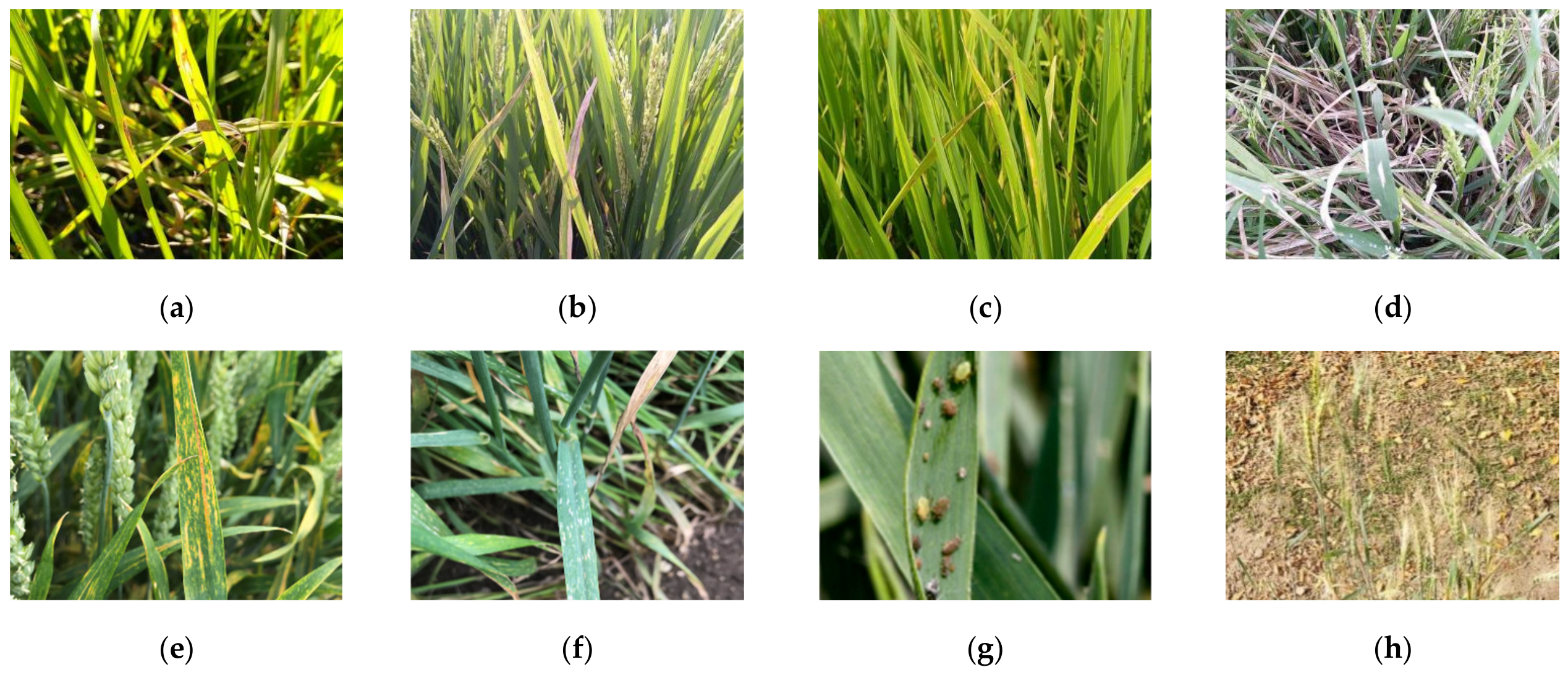Figure 1 shows representative diseases and insect pests of rice and wheat. These targets differ in symptom location, morphological scale, and contextual conditions. Diseases generally appear as color or structural abnormalities in leaves, sheaths, panicles, spikes, or the canopy, whereas insect pest monitoring must address insect bodies, feeding damage, and population density. Their associated algorithmic tasks therefore cannot be reduced to leaf-image classification alone.

The scope of existing literature is uneven; research on plant diseases tends to focus on classification, severity assessment, and mapping of affected areas, while research on insect pests places greater emphasis on small-object detection, insect counting, density grading, and migration trends. Localized disease lesions, spike symptoms, canopy anomalies, and insect targets correspond to different observation scales. Localized lesions are suitable for fine-scale segmentation, canopy anomalies for remote-sensing mapping, while insect targets are often constrained by size, overlap, and occlusion. Consequently, although disease and pest studies share image, spectral, and environmental data, their labeling formats, evaluation metrics, and the implications of their outputs still require separate discussion.

Disease-image recognition has shifted from conventional methods to deep learning [8]. Early research used manually designed color, texture, vegetation-index, and spectral features with PLS, SVM, RF, or XGBoost [9]. Recent reviews describe the same transition from conventional pipelines to deep learning [10]. Deep learning expanded the task to object detection [11], pixel-level segmentation [12], and multi-crop diagnosis [13], as well as dense insect counting [14]. Multimodal and time-series models attempt to combine phenotypic, physiological, environmental, and historical information in one inference process. However, some studies still rely on random sample partitioning and a single accuracy metric; training and test sets may share plots, equipment, backgrounds, or adjacent time points, limiting evidence for cross-region, cross-year, and cross-device use.

Recent reviews have addressed different aspects of intelligent crop disease and pest monitoring. Zheng et al. [3] reviewed remote-sensing monitoring of rice diseases and pests from different data sources. Wang et al. [10] summarized deep learning applications for plant disease and pest detection, whereas Yan et al. [11] reviewed lightweight detection in occluded fields. Ren et al. [15] reviewed deep learning segmentation in agricultural remote sensing, and Ouhami et al. [16] discussed computer vision, IoT, and data fusion for crop disease detection. These reviews provide valuable summaries; however, their scopes are mainly organized around a specific crop, sensing technology, algorithmic task, or monitoring system. Thus, this review primarily focuses on the issues of diseases and insect pests in rice and wheat, and then connects unimodal recognition, multimodal fusion, time-series prediction, and field robustness within a common framework. It further relates sensing signals and algorithmic tasks to crop growth stages and disease/pest progression. It also evaluates the strength of evidence beyond internal model accuracy by considering sample independence, external validation, missing modalities, and cross-location and cross-year generalization.

Reported model outputs include disease or pest classes, risk levels, lesion or insect locations, target counts, affected area, severity, and the probability or trajectory of future outbreaks. Classification, detection, segmentation, regression, and time-series forecasting provide different levels of information. Translating these outputs into field scouting, severity grading, risk assessment, and management actions still requires label conversion, threshold selection, external validation, and on-site verification. Studies that jointly record model outputs, management actions, and subsequent changes in yield or inputs remain scarce; algorithmic metrics therefore cannot substitute for evidence of production outcomes.

Against this background, this review reorganizes the evidence according to the sequence “data acquisition and characterization—unimodal recognition—multimodal fusion—time-series prediction—field robustness” [17]. It compares data foundations, algorithmic characteristics, model outputs, and validation evidence for classification, detection, segmentation, counting, severity estimation, and risk prediction [18]. Particular attention is given to sampling units, data partitioning, the net gain from fusion, missing modalities, probability calibration, cross-region and cross-year generalization, and computational and deployment burdens. The review then identifies gaps in presymptomatic monitoring, stability across growth stages, multisite and multiyear validation, and prospective trials linked to management decisions. Because the evidence base is considerably larger for diseases than for insect pests, disease identification and early warning form the main evidence chain. Insect detection is discussed in Section 2.1; small-target detection, counting, and density grading in Section 3.2; temporal forecasting of migratory pests in Section 5.1; and the shortage of cross-region and cross-year pest-warning evidence in Section 7.

2. Data Acquisition and Characterization for Rice and Wheat Disease and Pest Monitoring

2.1. Sensing Modalities and Observable Information on Diseases and Insect Pests

The inputs for pest and disease algorithms are not abstract “data”, but observable outcomes of pathogen infection, insect feeding, and host responses at different scales. Available information includes visible phenotypes such as the color, morphology, and texture of leaves and spikes, as well as boundaries between insect bodies and lesions [19]. Hyperspectral imaging reflects chlorophyll, water status, and biophysical stress, including red-edge changes [20]. Reviews of hyperspectral disease sensing explain the same physiological basis [21]. Thermal infrared and fluorescence capture transpiration, canopy temperature, and photosynthetic efficiency [22]; environmental records cover temperature, humidity, rainfall, and leaf wetness; pest and spore records describe population density, migration, and inoculum sources.

Common acquisition devices include visible-light cameras, multispectral and hyperspectral imagers, near- and short-wave-infrared spectrometers, thermal and chlorophyll-fluorescence imagers, gas sensors, and electronic noses [23], plus environmental nodes, insect traps, diffraction-based spore detectors [24], and polarization-based spore detectors [25]. Recent studies have further used microscopy-image features, diffraction fingerprints, impedance measurements, microfluidic enrichment, and Raman or SERS fingerprints for rapid crop-disease spore detection [26,27,28,29,30,31,32]. RGB data depict lesions, insect bodies, and tissue morphology; spectral data reflect pigments, water, and tissue structure; thermal and fluorescence data characterize transpiration and photosynthetic anomalies; environmental, pest, and spore data record conducive conditions and temporal dynamics.

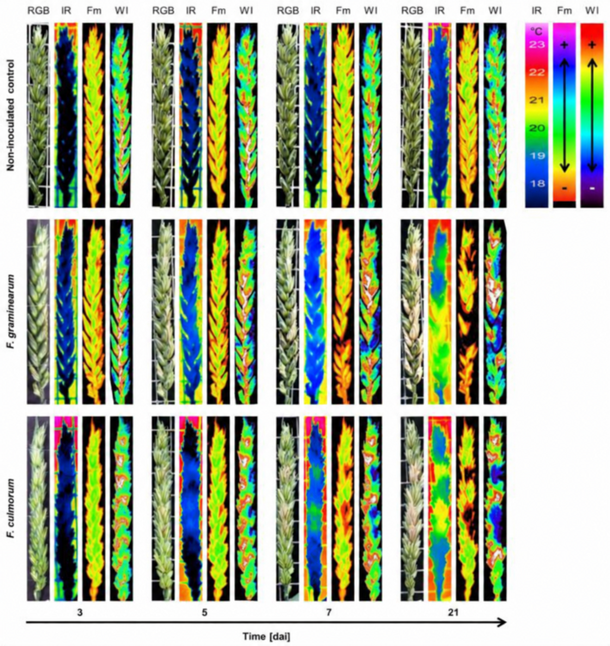
Mahlein et al. [33] monitored Fusarium head blight in wheat spikelets inoculated with Fusarium graminearum and Fusarium culmorum using repeated measurements with different imaging methods. As shown in Figure 2, RGB images show visible symptom development, infrared thermography shows temperature changes associated with infection, and chlorophyll fluorescence imaging shows changes related to photosynthetic activity. The water index (WI) derived from hyperspectral reflectance is related to tissue water content. The response times and sensitive areas of different modalities to disease progression are not entirely consistent, indicating that the value of multi-source monitoring lies in obtaining complementary phenotypic and physiological information, rather than simply increasing the volume of data.

Figure 2 illustrates the response of different imaging modalities to disease progression at the ear level; however, in practical monitoring, the same signal carries different implications at the leaf, plant, canopy, field, and regional scales. Single-leaf images facilitate background control and precise lesion segmentation, which may overestimate visibility under field conditions. Ground-based canopy and UAV imagery can characterize spatial heterogeneity, but labels are typically derived from a limited number of sample points and are susceptible to registration errors and canopy occlusion. Weather station and satellite data cover a large area but struggle to identify disease types on their own. Therefore, sensors, resolution, sampling frequency, and labeling scale must be matched to the sampling unit and the specific algorithmic task.

Sensing modalities differ in information content and acquisition constraints (

Table 1. Major sensing modalities and algorithmic tasks for monitoring rice and wheat diseases and insect pests.

Modality	Signal	Tasks	Strength	Limitation
RGB/visible	Color, shape, texture	Classification; detection; segmentation; counting	Low cost; mobile-ready	Sensitive to illumination, occlusion, and background
Multispectral/hyperspectral/NIR	Reflectance, red edge, sensitive bands	Early detection; severity regression; mapping	Rich physiological information	High dimensionality; calibration and transfer challenges
Thermal/fluorescence	Temperature, transpiration, photosynthetic efficiency	Physiological anomaly screening	May detect presymptomatic responses	Limited disease specificity
Environmental/meteorological/IoT	Temperature, humidity, rainfall, leaf wetness	Risk forecasting; time-window identification	Continuous monitoring	Cannot identify the causal disease alone
Trap/pest imagery	Insect bodies, counts, migration trends	Detection; counting; population warning	Captures pest dynamics	Small targets; overlap; maintenance
Spore/biosensors	Pathogen/inoculum signals	Source monitoring; auxiliary confirmation	Strong pathogen relevance	Limited sampling coverage and field integration

). RGB imaging supports wheat [34] and rice diagnosis [35], including mobile false-smut recognition [36]. Photothermal fusion enables presymptomatic rice-blast perception [37], whereas RGB supports field object detection [38]. RGB methods remain sensitive to illumination, shadows, background, and occlusion, and often become reliable only after lesions form. Multispectral and hyperspectral sensing captures canopy/red-edge responses in rice blast [39], SPAD shifts under bacterial leaf blight [40], and near-infrared responses in wheat powdery mildew [41]. FTIR-PAS detects incubation-stage rice blast [42], while hyperspectral sensing identifies narrow-band wheat leaf-blotch patterns [43] and other early signals [44]. Hyperspectral models have also detected early rice disease [45] and asymptomatic bacterial leaf blight [46]. These sensors support severity regression [47], sensitive-band selection [21], and field mapping, but equipment cost, calibration, redundancy, and cross-device transfer remain obstacles. Recent reviews also summarize non-destructive plant-disease detection across spectral, imaging, UAV, and AI methods [48].

Thermal infrared and chlorophyll fluorescence can reflect transpiration [49] and photosynthetic abnormalities [22], complementing visual and spectral data. However, water stress, heat stress, and canopy structure can produce similar responses, limiting disease specificity. Host and environmental data support dynamic wheat Fusarium head blight prediction [50]. In other crops, weather sequences support disease prediction [51], and spore observations support transmission analysis [52]. Trap-based monitoring targets population dynamics [53], while image methods estimate planthopper density through AR-assisted detection [54] and field counting [55]. No modality is universally superior; suitability depends on signal specificity, resolution, cost, calibration, and cross-device consistency.

RGB imagery supports classification, detection, and segmentation once visible symptoms are present. Multispectral, hyperspectral, and near-infrared data are more commonly used for sensitive-band analysis, severity regression, and spatial mapping, whereas thermal infrared and fluorescence data primarily support physiological anomaly screening. Environmental time series and pest-monitoring data support outbreak-risk forecasting and population-trend analysis, respectively. No sensing modality is universally superior. Suitability depends on the target task, signal specificity, spatiotemporal resolution, acquisition cost, calibration requirements, and cross-device consistency. Comparisons between sensing approaches should therefore account for sampling scale, calibration, label quality, and data partitioning so that differences in experimental conditions are not incorrectly attributed to the sensing modality itself.

2.2. Data Preprocessing, Feature Extraction, and Chemometric Methods

As different types of sensor data have varying data structures and sources of error, appropriate data preprocessing is required prior to pest and disease identification. Hyperspectral, near-infrared, and multivariate environmental data typically have high dimensionality, strong variable correlations, and complex noise structures; smoothing, standard normal variate (SNV) transformation, scatter correction, baseline correction, and derivative transformation can be used to mitigate noise, scatter, and drift. UAV and multitemporal data also require radiometric correction and geometric registration. RGB data emphasize color consistency and background control; thermal infrared data require temperature calibration and environmental compensation; while pest counting necessitates handling of small targets, overlap, and occlusion. If preprocessing parameters are estimated using the entire dataset before data splitting, information from the test set can leak into model development and lead to overly optimistic performance estimates. Therefore, preprocessing parameters should be fitted using the training set only and then set unchanged for the validation and test sets.

These methods serve different purposes. SPA, CARS, VIP, and genetic algorithms can be used for variable selection to identify informative spectral variables [39]. Similar screening of sensitive spectral variables has also been used for early disease detection [56]. PCA is mainly used for dimensionality reduction by transforming correlated variables into a smaller number of principal components. In contrast, PLSR, PCR, LDA, and PLS-DA are used for predictive modeling [41]. Regression models can be used for disease severity estimation [43], while classification models can be used to distinguish different disease or pest levels [57]. Variable-selection methods help reduce redundant information, whereas dimensionality-reduction methods simplify the data structure. Predictive models use the processed variables to estimate or classify the target. Their performance may still be affected by preprocessing, sample composition, and differences among datasets.

Traditional statistical and chemometric methods remain useful in current research. PCA is mainly used for dimensionality reduction, whereas PLSR and PLS-DA can serve as regression and classification baselines, respectively. These methods are particularly useful when sample sizes are limited or when interpretability of the model is important. Relevant literature typically begins by analyzing the relationship between spectral bands or indices and disease status, before selecting SVM, RF, XGBoost, or deep learning models based on sample size and the degree of non-linearity; such comparisons help distinguish whether performance improvements stem from new features, non-linear modeling, or the scale of the data.

2.3. Algorithmic Tasks, Label Generation, and Data Quality

The sensing modality constrains the information available to the model. RGB imagery is commonly used for symptom classification and spatial localization; hyperspectral data support sensitive-band analysis and the detection of early physiological abnormalities; environmental data support modeling of outbreak conditions and temporal risk; and pest-monitoring terminals focus on abundance and population trends. Severity quantification requires labels for lesion area, the proportion of affected panicles or spikes, canopy indices, or pest density. Risk forecasting requires continuous time-series records and a clearly defined forecast origin. Studies spanning fields or devices should also retain metadata on location, year, cultivar, equipment, and management practices.

Models based on one primary sensing modality are considered unimodal, even when they combine color, texture, or multiple spectral indices. Multimodal fusion requires the joint modeling of heterogeneous evidence, such as RGB imagery, spectral or thermal measurements, environmental records, and pest-monitoring data.

In addition to the input modalities, the method of label generation and the quality of the dataset also determine model performance. Leaf disease classification can be confirmed by experts; lesion segmentation requires clear boundary rules; and disease severity also involves grading criteria, the number of sample plots, and the time of survey. Pest counts are easily affected by clumping, occlusion, and different developmental stages, while remote sensing labels are often extrapolated from a small number of ground survey points to canopy pixels. The error structures of different labels vary and cannot be uniformly regarded as completely correct “ground truth”.

Existing datasets vary in the extent to which they retain information at the original object level. Image data recorded at the plot, plant, leaf, or ear level, as well as remote sensing and time-series data that retain flight information, sampling points, geographical location, and sampling time, make it easier to identify duplicates across datasets for the same object or adjacent scenes; in the absence of such metadata, data leakage caused by random partitioning is often difficult to trace.

Some pest and disease datasets show uneven class distributions. For example, IP102 has a pronounced long-tail distribution [58]. Mild-symptom or low-density samples may also be underrepresented in some datasets, but this information is not consistently reported. Therefore, class distribution and model performance across different symptom-severity or pest-density levels should be reported when available.

There are marked differences in the comprehensiveness of reporting regarding sample units, label sources, and data partitioning across existing studies. High-accuracy results that fail to specify the original object hierarchy, the label formation process, and the training–testing partitioning method primarily reflect internal recognition capabilities under specific data conditions; in contrast, tests involving cross-expert consistency, independent field plots, and samples spanning multiple years and challenge conditions are better suited to revealing a model’s stability under varying labels and scenario shifts. In the current literature, the latter type of study remains significantly less common than random internal partitioning.

The composition of publicly available datasets further reflects these data-quality and validation issues. Existing research on plant pest and disease recognition has established general-purpose benchmarks such as PlantVillage and IP102, while several crop-specific datasets for rice and wheat have also been developed. The datasets listed in

Table 2. Illustrative public and benchmark datasets used for intelligent monitoring of rice and wheat diseases and insect pests.

Dataset	Modality/Setting	Size	Classes	Access
PlantVillage [59]	RGB; controlled detached leaves	54,306 images; 38 classes	26 diseases; 14 crops; no rice/wheat	Yes
IP102 [58]	RGB; natural backgrounds; box-annotated subset	75,222 images; 102 classes; ~19,000 box-annotated	Crop pests, including rice/wheat pests	Academic use
Paddy Doctor [4]	RGB; smartphone field images	16,225 images; 13 classes	12 rice disease/pest classes + healthy	Yes
Rice Leaf Disease Image Samples [60]	RGB; field images	5932 images; 4 classes	Bacterial leaf blight, blast, brown spot, tungro	Yes
WDD2017 [34]	RGB; wheat fields	9230 images; 7 classes	6 wheat diseases + healthy	No
WFD2020 [61]	RGB; natural field images	2414 images	Leaf/stem/stripe rust, powdery mildew, leaf spot	Yes

Note: PlantVillage does not contain rice or wheat classes but is included because it is widely used for pretraining and benchmarking plant-disease recognition models.

were selected based on their common use in previous studies, their relevance to rice and wheat disease or pest monitoring, and their different acquisition settings and class structures. Table 2 is intended to be illustrative rather than comprehensive.

Table 2 shows that existing benchmark datasets still consist primarily of RGB images and classification labels, while the availability of multispectral, hyperspectral, thermal infrared, environmental time-series, and spore data remains significantly limited. RGB datasets are mainly suitable for low-cost recognition and localization of visible disease symptoms and insect pests. Although PlantVillage is a large-scale dataset, it uses detached leaves against relatively uniform backgrounds and excludes rice or wheat; IP102 covers a wide range of pest categories but exhibits a pronounced long-tail distribution; datasets dedicated to rice and wheat are generally constrained by factors such as a single location, a single imaging modality, or a limited sample size. Although datasets such as WDD2017 have been used for method validation, they have not been fully released, further limiting the reproducibility of results and the ability to make uniform comparisons. Therefore, when evaluating models using publicly available datasets, it remains necessary to report the original sample units, collection locations and years, equipment, class distribution, annotation methods, and training–testing split strategies.

2.4. Growth Stages, Symptom Progression, and Monitoring Tasks

Observable signals vary with crop growth and disease or pest progression. Before symptoms appear, informative signals include conducive conditions [50], pathogen or pest activity [53], and changes in chlorophyll [39], water status [40], temperature [49], and fluorescence [22]. Environmental time series [62], spore or pest records, and spectral data [45] therefore support risk forecasting and anomaly detection. Once symptoms develop, lesion color and morphology [3], panicle or spike symptoms [63], and insect targets become more distinct. Visible symptoms support RGB classification [64], ground/UAV yellow-rust detection [65], multispectral aerial monitoring [66], yield-linked early detection [67], and segmentation. MOS arrays detect symptomless rice-blast VOCs [68]. VOC- and odor-based sensing has also been applied to early warning of rice mildew and stored-wheat mildew [69,70]. During progression, affected panicles or spikes [71], canopy indices [72], and pest density [73] provide labels for severity regression [74], counting [54], regional wheat-stripe-rust mapping [75], and field-scale rice bacterial leaf blight mapping [76].

Table 3. Growth-stage-specific monitoring targets, signals, tasks, and evidence gaps for rice and wheat diseases and insect pests.

Parameter	Seedling	Tillering–Jointing	Heading–Flowering	Grain filling–Maturity
Rice targets	Seedling blast; early bacterial leaf blight; initial pests.	Blast; sheath blight; leaf folder; planthoppers.	Neck blast; false smut; migratory pests (e.g., brown planthopper).	Progressing blast/sheath blight; late pests.
Wheat targets	Early stripe rust/powdery mildew; Aphids.	Stripe rust; powdery mildew; aphids.	Fusarium head blight; stripe rust; aphids.	Progressing Fusarium head blight; late rust/mildew.
Signals	Microclimate; leaf wetness; spores/insects; RGB/spectra.	Leaf/sheath RGB; canopy spectra; UAV images; insect counts.	Weather; spores/insects; panicle/spike RGB, spectra, thermal.	Lesion area; canopy spectra/thermal; yield traits.
Tasks	Risk prediction; anomaly screening; early classification.	Classification; pest detection/counting; severity mapping.	Early warning; panicle/spike detection; severity grading.	Severity mapping; progression/yield-loss analysis.
Evidence gaps	Few multisite, multiyear presymptomatic studies.	Limited cross-cultivar/stage and occlusion tests.	Few prospective multiyear trials.	Weak cross-stage transfer and disease–senescence separation.

summarizes the major targets, signal progression, and algorithmic tasks across the growth stages of rice and wheat. Changes in leaf color and canopy structure during the seedling and tillering/jointing stages can be confounded by nutrient status, water stress, or cultivar differences. Panicle and spike diseases during heading and flowering are closely associated with warm and humid conditions, whereas natural senescence during grain filling/maturity reduces the specificity of color and spectral features. Early warning, symptom classification, and severity estimation are therefore complementary tasks associated with the presymptomatic, visible symptom, and damage progression stages, respectively.

Available evidence appears to be uneven across growth stages. Evidence remains limited for presymptomatic seedling monitoring, disease–senescence discrimination at grain filling/maturity, and cross-stage transfer. This pattern reflects a qualitative synthesis of the representative literature reviewed here rather than a formal bibliometric comparison, because growth-stage information is not consistently reported across studies. These gaps require stage-specific tasks and validation.

3. Unimodal Monitoring Algorithms: From Handcrafted Features to Deep Representation Learning

Unimodal algorithms form the basis for the intelligent monitoring of rice and wheat pests and diseases. Their inputs may include RGB images, hyperspectral cubes, UAV multispectral imagery, thermal infrared images, or environmental time series; however, during a single inference, the model relies primarily on a single information modality. Relatively abundant data are available for unimodal studies. These data provide a useful baseline for evaluating whether multimodal fusion offers additional benefits.

The same algorithm encounters varying levels of symptom visibility, canopy structure, and labeling scale across different growth stages; consequently, subsequent quantitative comparisons must also take into account the growth stages or disease progression stages covered by the research.

Unimodal tasks can be categorized into classification, regression, object detection, segmentation, and counting. Classification determines which type of pest or disease a sample belongs to, or its risk level; regression estimates disease indices, lesion proportions, or pest densities; object detection pinpoints the locations of lesions, diseased spikes, or pests; segmentation further identifies affected areas at the pixel level; counting targets dense, small objects such as planthoppers. Metrics for different tasks are not interchangeable. Classification accuracy does not indicate localization quality, detection mAP does not directly represent errors in severity estimation, and segmentation IoU does not automatically equate to field disease severity ratings.

The strength of evidence from unimodal studies is primarily influenced by sample units, acquisition scenarios, class distributions, data partitioning, and external validation. If adjacent samples from the same leaf, the same spike, or the same drone flight path are randomly assigned to the training and test sets, higher metrics are more indicative of recognition within that specific distribution rather than generalization to field conditions. Existing literature often reports only overall accuracy, while disclosure of recall rates per class, the number of false negatives, confidence levels, and failed samples is relatively insufficient, making it difficult to assess the recognition thresholds for high-risk categories.

3.1. Disease and Pest Classification and Severity Assessment: From Traditional Machine Learning to Deep Learning

Traditional machine learning research typically uses color, texture, morphology, vegetation indices, sensitive bands, and environmental statistics as inputs. UAV monitoring of rice sheath blight [47], hyperspectral analysis of wheat powdery mildew [41], UAV hyperspectral mapping of Fusarium head blight [71], and UAV multispectral monitoring of wheat scab [77] represent tasks such as classification, severity regression, and spatial mapping, respectively. SVM [57] is suitable for small to medium-sized samples and high-dimensional features, while RF [39] provides variable importance and reduces overfitting in individual trees; XGBoost and GBDT [78] are used to capture non-linear relationships and feature interactions. These studies demonstrate that the role of manually feature-engineered models extends beyond providing a benchmark for accuracy to include testing whether sensitive variables exhibit stability across samples and scenarios.

The main advantages of these methods are their low training costs, relatively modest sample size requirements, and the ability to interpret feature contributions through methods such as variable importance, partial dependence, and SHAP. For portable spectroscopic devices, low-cost sensors, and small-scale field trials, traditional machine learning remains highly practical. However, their performance ceiling is constrained by the quality of the manually engineered features: subtle symptoms, complex backgrounds, and compound stresses are often difficult to describe using fixed colors or textures, while differences in region and equipment may also affect the stability of spectral bands and indices.

In existing research, traditional machine learning continues to serve as the interpretable baseline. Some deep learning models achieve only limited internal gains compared to Random Forests (RFs) or Support Vector Machines (SVMs), while increasing the burden of labeling and computation; other simplified models, however, maintain more stable results under conditions of small to medium sample sizes. Due to significant variations in data splitting and external testing conditions across studies, direct comparisons remain difficult. The reviewed studies show mixed results. The relationship between model complexity and cross-scenario generalization still remains unclear.

Compared with models based on manually derived features, deep learning expands feature representation through end-to-end learning [79]. CNNs [9], ResNet [80], DenseNet, EfficientNet, and MobileNet learn multilevel features from leaf, panicle, spike, and canopy images. In other crops, multiple CNN architectures have been compared for real-time field disease classification [81]. Self-supervised Transformer pretraining supports pest and disease classification [82], while multiscale feature fusion supports fine-grained disease categorization [83]. Image- and point-cloud models extend representation to plant-protection tasks [84]. Mobile false-smut recognition [36], field maize leaf blight detection [38], multidisease rice diagnosis [80], and multi-crop disease identification [13] illustrate visible-image applications. However, dependence on visible symptoms, device variation, and outdoor degradation remains common. Models may exploit background, device, or acquisition-batch cues, so automatic representation does not guarantee stable generalization.

Under identical dataset and data partitioning conditions, the performance gap between traditional hand-engineered features and deep representations becomes even more pronounced. Wu et al. conducted a comparison using a unified training, validation, and test split on the IP102 pest dataset [58]; the classification accuracy of SURF features combined with an SVM was 19.5%. The ResNet model achieved an accuracy of 49.4% on IP102. Its F1 score and G-mean were 40.1% and 31.5%, respectively. In this comparison, ResNet outperformed the SURF–SVM baseline; however, class imbalance remained a challenge. Using 5932 field images of rice diseases, Sethy et al. [60] further compared approaches such as manual features (LBP, HOG, and GLCM) combined with SVM, end-to-end transfer learning, and deep features combined with SVM. Among these, the combination of ResNet-50 deep features and SVM achieved an F1 score of 0.9838, outperforming the manual feature models overall. These results indicate that the primary benefit of deep learning stems from improved feature representation capabilities; however, internal advantages observed on a single dataset cannot replace validation across different locations, devices, and years.

Mobile and embedded applications [85] have driven the development of lightweight models [37], transfer learning, pruning, and quantization. While lightweight models can reduce the number of parameters and inference latency, if the training data are derived primarily from clean backgrounds, the compressed models may still fail under conditions involving reflections, occlusions, and weak symptoms. Current studies on lightweight models mainly focus on parameter count and inference speed. Device type, input size, memory use, offline operation, and external test results are less consistently reported.

3.2. Object Detection, Lesion Segmentation and Quantification

MA-YOLO uses multiscale fusion and attention for pest detection [86]. GDFC-YOLO is used for wheat disease detection [87]. Similar YOLO-based methods have also been studied in other crops [88]. Such studies are cited only as methodological references. Two-stage and single-stage agricultural detectors [11] output class and location information for lesions, diseased panicles or spikes, insect bodies, and damaged areas [89]. A multiscale SSD-based field detector [38] and GDFC-YOLO [87] localize diseased leaves or wheat-disease targets under complex backgrounds. Dense planthopper counting further extends detection to abundance and density. Single-stage models generally infer faster, whereas two-stage models process candidate regions in more detail. Differences in input size, hardware, and test sets still prevent direct cross-study comparison.

Insect counting faces challenges such as high target density, small size, similar poses, and severe occlusion. Density map regression, fully convolutional counting [14], and detection–tracking combinations [54] can reduce reliance on individual bounding boxes, but errors vary with density ranges, image quality, and the degree of occlusion [55]. Most existing studies report average counting errors at the single-image or plot level, with few further verifying the consistency of counting results with field survey thresholds or density classifications across growth stages.

In addition to object detection and counting, pixel-level segmentation further extends the identification results to the quantification of lesion extent and severity [90]. Common segmentation architectures include U-Net [91], DeepLabv3+ [92], Mask R-CNN [93], and SegFormer [94]. These architectures support pixel-level or instance-level segmentation. Related U-Net-based applications have also been reported in other crop-protection tasks [95]. In wheat, multiscale imaging and segmentation approaches have been discussed for Fusarium head blight detection [96]. Segmentation is closer to severity quantification than classification, but pixel annotation is costly, and lesion boundaries are often influenced by leaf veins, shadows, reflections, and expert judgement. Differences in boundary delineation between annotators may be comparable to performance differences between models, yet existing research remains insufficient in reporting annotation protocols, the number of experts involved, and consistency results.

Severity estimation also involves a scale conversion from pixel proportions to agricultural disease severity classes. The area of localized leaf lesions, the degree of damage to the entire plant, and the field-scale disease severity index are not equivalent labels and cannot be directly interchanged. Relevant studies typically report image-level area errors, disease severity classification results, or plot-scale correlations separately; in the absence of independent manual surveys or cross-plot validation, pixel-level segmentation accuracy cannot be directly interpreted as the accuracy of field-scale severity measurements.

3.3. Spectral and Remote Sensing Unimodal Modeling

In hyperspectral and multispectral research, traditional machine learning and deep learning models are often used in tandem. Rice sheath blight [47], wheat powdery mildew [41], and Fusarium head blight [71] studies use bands, indices, and texture with SVM, RF, PLSR, or XGBoost; FTIR-PAS also enables incubation-stage rice-blast diagnosis [42]. Notably, 1D CNNs [21], 2D CNNs [45], and 3D CNNs [46] process spectral sequences, spatial texture, and spectral–spatial joint features [97], respectively. The combination of indices and texture within the same multispectral image constitutes feature fusion within a single remote sensing modality; the resulting performance improvement cannot be directly taken as evidence of complementarity between heterogeneous sensors.

UAV [64] and satellite data [75] can be used to generate spatial distribution maps of plant diseases, but the number of labels is typically far fewer than the number of pixels [98]. Randomly partitioning adjacent pixels within the same field is subject to strong spatial autocorrelation, while directly extrapolating ground-based small-plot labels to large-scale canopy areas [76] may also introduce scale errors. Studies using fields, flight campaigns, regions, or years as partitioning units are better able to reduce the optimism bias caused by spatial dependence. A single-site UAV study further showed that interridge soil and shadow backgrounds can materially affect multispectral FHB monitoring [63].

3.4. Comparison of Unimodal Algorithms, Model Interpretation and Error Analysis

Existing unimodal studies exhibit significant differences in terms of task type, data scale, and validation depth. Classification models primarily output disease or pest categories or severity levels; object detection models further provide the locations of lesions, diseased spikes, or insect bodies; spectral and remote sensing models more frequently output severity levels, threshold categories, or spatial probability distributions. The metrics reported across studies are also task-dependent. In this review, accuracy denotes the proportion of correctly classified samples, whereas OA refers to overall accuracy as reported in the original studies. Although the two may be numerically equivalent in standard single-label classification, the original terminology is retained because their definitions and evaluation settings may vary across studies. Accordingly, accuracy, F1 score, mAP, and OA should not be directly compared across studies without considering the sample units, test scenarios, and validation methods. The numerical results summarized in

Table 4. Representative quantitative evidence, model outputs, and application validation status of unimodal algorithms for rice and wheat monitoring.

Target/Ref.	Data/Validation	Model/Task	Key Result	Output/Use	Validation
Rice diseases [80]	33,026 images; 4 sites/2 years; 300 external; stages variable.	DL classifier	Internal >99%; external 91%; F1 0.83–0.97.	Class/confidence; mobile screening.	External sites/years; management untested.
Rice BLB [98]	3 fields; 658 train + 120 external; stages unspecified.	UAV-MS mapping	OA 92.3% internal; 80.0% external.	Disease-probability map; field check.	Cross-site/year; no prospective trial.
Rice leaf folder [89]	222 quadrats; 2 stages.	UAV-HS + XGBoost grading	accuracy 87.46% same-stage; 86.0% cross-stage.	Severity + hotspots; prioritize inspection.	Cross-stage; action thresholds untested.
Wheat leaf blotch [43]	1 ha; 335 cultivars; external 331 cultivars/758 observations; stage unreported.	PLS-DA	Sensitivity 95.83%; specificity 92.68%; OA 92.88%.	Severity/spectral separation; resistance screening.	External cultivars; manual-rating comparison.
Wheat FHB [71]	50 plots × 2 dates (100 samples); 80:20 split; 5-fold CV; filling stage,	UAV-HS spectral + texture + color; RF	Prediction 85%; 5-fold CV 83%.	3 severity classes + map; field check.	One field/year; random split; no management trial
Multiple wheat diseases [87]	4156 images/5845 instances; 1130 external; stage unreported.	GDFC-YOLO	mAP50 0.900 internal; 0.920 external.	Lesion class/location; field verification.	External images; no prospective test.
Wheat aphids [57]	431 canopy spectra; 8 plots; 3 stages.	SVM/RF/LGBM	F1 0.89–0.99.	Threshold class; prioritize inspection.	Manual counts; no cross-field or forward trial.

Note: BLB, bacterial leaf blight; FHB, Fusarium head blight; MS, multispectral; HS, hyperspectral; LGBM, LightGBM; OA, overall accuracy. Numerical results are reported as presented in the original studies and should not be interpreted as directly comparable performance rankings across studies.

are therefore intended to illustrate the evidence reported in individual studies rather than to provide a direct ranking of model performance across studies. Representative studies also indicate that there are typically intermediate steps—such as manual surveys, threshold conversions, and on-site verification—between the model’s direct output and its potential applications. Accordingly, Table 4 summarizes quantitative metrics, direct model outputs, potential task associations, and application validation status to distinguish between capabilities that have been validated and uses that have not yet been confirmed through field trials. The numerical results summarized in Table 4 are therefore intended to illustrate the evidence reported in individual studies rather than to provide a direct ranking of model performance across studies.

Table 4 provides three illustrative observations from the representative studies summarized here. Firstly, strong internal results do not necessarily transfer to independent external data. The rice multi-disease classifier exceeded 99% accuracy internally but declined to 91% on external images; the OA of the rice bacterial leaf blight model decreased from 92.3% to 80.0% in cross-location and cross-year testing. By contrast, GDFC-YOLO maintained a high mAP on external field images acquired under similar conditions, showing that the strength of external evidence depends on independence in location, year, equipment, and background. Secondly, different tasks produce different direct outputs: classifiers provide classes or severity levels, detectors provide classes and locations, and spectral or remote-sensing models provide damage levels, severity estimates, or spatial probability maps. These outputs may support field reinspection or survey prioritization, but “mobile prescreening,” “targeted reinspection,” and “treatment-area delineation” remain potential uses rather than validated management outcomes. Thirdly, among the representative studies summarized in Table 4, application validation is often limited to comparisons with manual surveys and a small number of cross-site or cross-year tests. Prospective trials that jointly record model outputs, survey effort, intervention timing, and input changes are not commonly reported in these studies.

The discrepancies between internal and external performance reflected in Table 4, as well as the gap between direct outputs and potential applications, illustrate that a single accuracy metric is insufficient to determine whether a model has generated stable and reliable information on plant diseases and pests. In addition to quantitative results, the areas or spectral bands targeted by the model, the reliability of the output probabilities, and the sample conditions in which errors are concentrated constitute a further layer of evidence for comparing unimodal algorithms. Following a comparison of the quantitative performance of different models, model interpretation and probability calibration provide another set of evidence for assessing the credibility of the results. The interpretation methods for unimodal models must correspond to the data type. For image classification, Grad-CAM, occlusion experiments, and counterfactual perturbations can be used to check whether the model focuses on disease lesions and insect bodies; for spectral models, band importance, SHAP, and sensitivity analysis can be used to assess whether the model relies on physiologically significant bands; and for remote sensing models, spatial responses can be compared with ground-truth disease samples. If interpretability results lack ablation analysis, expert review, or validation on external samples, they typically only indicate the areas of interest in the model’s correlation analysis and cannot serve as evidence of causal or physiological mechanisms.

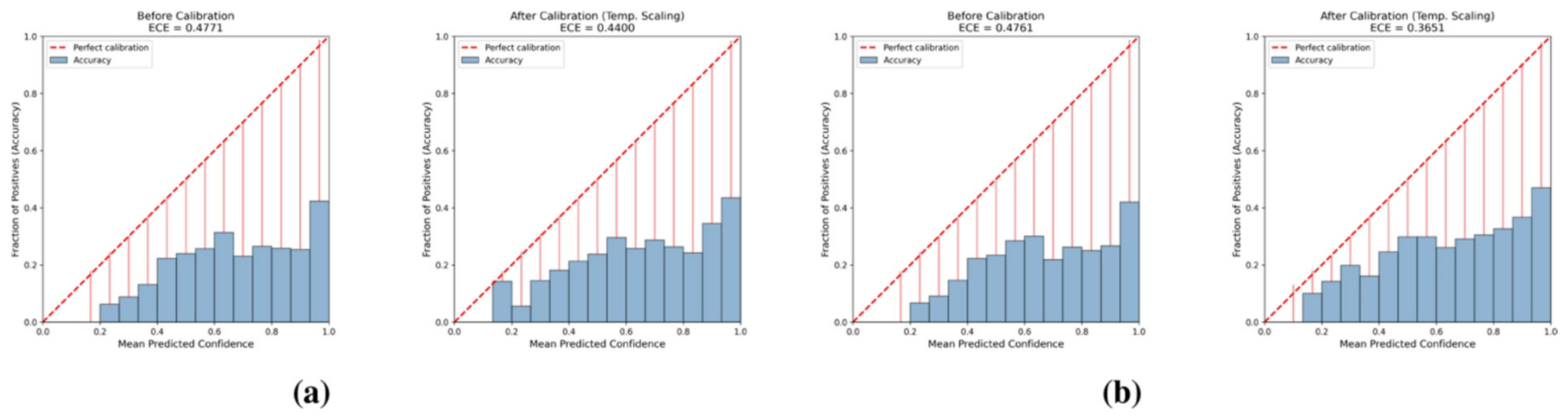
Confidence scores provide additional information about model outputs that distinguishes them from class labels. Deep learning models may assign excessively high probabilities to unfamiliar backgrounds and unknown disease types; methods such as reliability plots, expected calibration error, and temperature scaling can be used to assess the consistency between predicted probabilities and actual accuracy rates. Under conditions of weak symptoms, low pest density, and severe shading, the verification threshold alters the balance between false negatives and false positives; existing studies are inconsistent regarding threshold selection and the reporting of stratified results on independent validation sets.

Error analysis requires distinguishing between biological confounders and imaging artifacts. The former includes symptom similarity between diseases and similarity between diseases and non-disease stresses such as nutrient deficiency and senescence, while the latter includes shadows, reflections, blurring, and device-specific color variations. Reporting errors grouped by symptom intensity, background type, cultivar, growth stage, and device helps determine whether performance limitations stem primarily from data coverage, label definitions, acquisition conditions, or model architecture.

Overall, the variations in external performance, application validation status, and error types summarized in Table 4 suggest that the limitations of unimodal methods do not stem entirely from model structure. Confusion caused by weak symptoms and non-disease-related stresses reflects a lack of visible phenotypic information, which may be supplemented by spectral, physiological, or environmental data; errors resulting from variations in exposure, device differences, and background shifts, on the other hand, rely more heavily on acquisition calibration, data augmentation, and domain adaptation. Consequently, the rationale for multimodal fusion should be based on the causes of unimodal failure and the independent contributions of newly added information, rather than simply increasing the number of sensors or features.

4. Multimodal Data Fusion Algorithms

Plant diseases and insect pests alter appearance [99], physiology [39], temperature [49], and environmental responses [62], whereas a single modality captures only part of this evidence. Multimodal fusion [16] should align complementary data types before joint inference. Studies in other crops, including strawberry [100] and mulberry [101], are cited here only as methodological examples of multi-sensor fusion and are not treated as direct evidence for rice or wheat. Hyperspectral-terahertz fusion for tomato leaf mildew detection offers another cross-crop example of heterogeneous sensor fusion [102]. RGB images depict visible lesions, hyperspectral data reflect pigment and water-status changes, environmental records describe epidemic conditions, and monitoring terminals track pest populations. Fusion is meaningful only when these inputs refer to the same field, time point, and disease-severity label.

Growth stages also alter the complementary relationship between different modalities. The presymptomatic stage relies more on environmental and physiological signals, whereas the symptomatic stage relies more on RGB morphological information, and the disease expansion stage requires quantitative information. The disease expansion stage requires quantitative information such as lesion area, canopy structure, or pest density.

4.1. Multimodal Concepts, Data Alignment, and Quality Control

The terms “multi-source”, “multiscale”, “multitemporal”, and “multimodal” are often used together, but they describe data origin, spatial hierarchy, temporal coverage, and information type, respectively. Distinguishing them prevents within-modality feature enrichment, cross-platform integration, and heterogeneous fusion from being treated as equivalent. The four concepts are defined below.

(1) Multi-source describes where data are acquired. Data collected with different sensors, devices, or platforms are multi-source, but the modalities may be either identical or different. Ground cameras and UAV cameras, for example, both acquire RGB images; the platforms differ, but the information remains within the visible-light modality. Therefore, this is multi-source, single-modality data rather than multimodal fusion. Integrating such data primarily requires control of device response, acquisition parameters, and cross-platform domain shifts.

(2) Multiscale describes the spatial scale of observation. Rice and wheat diseases and insect pests can be monitored at the leaf, plant, canopy, field, and regional scales, each with different observation units, spatial resolutions, and label meanings. Single-leaf images support lesion classification and fine segmentation; canopy and UAV imagery support disease mapping; and satellite data support regional risk monitoring. Feature pyramids or different convolution kernels applied to one image constitute model-level multiscale feature extraction, not observations across leaf, canopy, and field scales. Thus, cross-scale fusion requires explicit correspondence between spatial coverage and disease labels.

(3) Multitemporal describes when observations are made. Repeated measurements of the same field, plant, or disease-progression unit at different growth stages, days after infection, or monitoring dates form a temporally continuous record. For example, repeated RGB, spectral, or meteorological observations of Fusarium head blight from heading through grain filling/maturity can capture infection, symptom development, and disease spread. Samples collected on different dates but not traceable to the same object or field represent temporal variation, not a disease-progression sequence. Multitemporal analysis therefore depends on consistent sampling intervals, preserved object identity, and accurate time labels.

(4) Multimodal describes what information the data provide. Fusion is multimodal when inputs arise from distinct sensing modalities that provide heterogeneous information. Features derived from an existing modality, such as vegetation indices calculated from multispectral bands, may constitute an additional input branch but are not treated as an independent sensing modality. RGB captures lesion color, morphology, and insect targets; hyperspectral data characterize pigments, water, and tissue structure; thermal infrared reflects canopy temperature and transpiration; environmental time series describe conducive conditions; insect or spore records describe inoculum and population change. Same-platform multispectral UAV studies combine bands and spatial features for yellow-rust monitoring [66] and early detection/yield assessment [67]. Six MOS channels support symptomless rice-blast detection [68] but, as one VOC-response class, are treated as within-modality fusion; spectral–texture–color features from one UAV hyperspectral source are likewise within-modality [71]. The central question is whether heterogeneous inputs provide complementary biological evidence, not whether they merely increase dimensionality.

These four attributes may coexist, but they are not interchangeable. For example, ground-based and UAV RGB imagery are both multi-source and multiscale but remain within a single modality. Repeated UAV RGB acquisition of the same field is multi-source, multiscale, and multitemporal, but it is still not multimodal. Heterogeneous multimodal observations arise only when distinct information sources such as spectral, thermal, environmental, or pest records are added. A study should therefore be described as multimodal on the basis of information heterogeneity, not merely the number of sensors, features, or acquisition dates.

The conceptual boundaries outlined above directly influence the interpretation of fusion gains. Performance improvements resulting from the addition of features within the same modality indicate a more comprehensive representation of those features, but do not directly prove complementarity between heterogeneous sensors; when acquisition times across different platforms are inconsistent, so-called fusion gains may also stem from disease progression or sampling bias. In the absence of clarification regarding data format, acquisition scale, and synchronization methods, it is difficult to attribute fusion gains to multimodal complementarity.

Once conceptual boundaries have been clarified, multimodal modeling also requires the establishment of reliable data correspondences. Specifically, temporal synchronization, spatial registration, radiometric calibration, resolution matching, and label consistency all influence the fusion results. Misalignment between UAV pixels and ground sampling points may result in healthy canopy being misclassified as diseased; furthermore, the average field conditions recorded by environmental sensors may not necessarily correspond to a single leaf image. If RGB and hyperspectral data are acquired on different dates, changes in disease progression may cause the one-to-one correspondence between modalities to be lost. Alignment errors often impose more direct constraints on results than the structure of the fusion network.

Quality control also encompasses missing values, low-quality modalities, and instrument drift. In practical fieldwork, it is not always possible to obtain a complete dataset; models trained on a full set of modalities may fail to operate when a particular sensor is missing. Some studies employ modality quality scoring, modality pruning, or reconstruction of missing modalities to enhance fault tolerance; however, there is as yet no unified reporting standard for results under conditions involving complete modalities, missing modalities, or synchronization errors.

4.2. Data-Level, Feature-Level, and Decision-Level Fusion

Data-level fusion involves channel concatenation, band stacking, or joint encoding at the raw or near-raw data level, thereby maximizing information retention. For example, registered RGB, thermal infrared, and multispectral pixels can be combined to form a multi-channel tensor, while continuous environmental sequences can also be fed into the network alongside remote sensing time series. Early-stage fusion is suitable for controlled experiments and mechanistic exploration but requires strict synchronization, sufficient sample sizes, and substantial computational resources.

Differences in the numerical ranges, noise structures, and dimensions of different modalities can result in one modality dominating the gradient, while high-dimensional spectra are also prone to overfitting under small-sample conditions. Consequently, data-level fusion typically requires normalization, dimensionality reduction, band selection, and modality balancing, while scene-level validation is employed to determine whether the model has learned genuinely complementary information.

Feature-level fusion first extracts modality-specific representations via independent encoders, then establishes cross-modal information exchange at the intermediate layers; the key lies not merely in “whether to fuse”, but in “where to fuse and how to allocate the contributions of different modalities”. In a cross-attention architecture, RGB features can be used as queries, while hyperspectral, thermal infrared, or environmental features serve as keys and values, enabling auxiliary modalities to supplement spectral, physiological, or environmental information in lesion areas in a targeted manner. Modality gating generates dynamic weights based on feature quality, prediction confidence, or missing data, suppressing low-reliability branches in situations such as high thermal infrared noise or incomplete environmental records. For multimodal Transformers, image patches, spectral vectors, and environmental variables can first be mapped to tokens of a unified dimension, with positional and modality encodings incorporated, before learning intra- and inter-modal dependencies via self-attention or cross-attention. Compared to direct concatenation, these architectures can select complementary information at the sample level but also rely more heavily on accurately paired data and sufficient training samples.

Direct rice/wheat evidence is provided by crop-specific fusion studies based on RustQNet and Rice-Fusion. Deng et al. [103] developed RustQNet, a three-branch fusion architecture that separately encodes UAV RGB imagery, multispectral imagery, and vegetation indices and enables feature interaction through cross-attention. Under the terminology adopted in the original study, these inputs were described as three modalities. In the present review, however, RGB and multispectral imagery are regarded as two distinct sensing modalities, whereas vegetation indices constitute a derived feature branch because they are calculated from spectral measurements. The RGB + MS + VI configuration achieved an R² of 0.8024, representing a 17.65–35.59% improvement over the single-input configurations reported in the original study. This result indicates improved predictive performance for the three-branch configuration in that study.

For smaller datasets, intermediate-layer fusion with simpler structures may prove more stable. For example, the Rice-Fusion model employs a CNN to extract features from rice images and an MLP to extract features from agrometeorological sensors, before performing joint classification via a feature concatenation layer and a fully connected layer. The model achieved a test accuracy of 95.31%, which is higher than that of the CNN model using only images (82.03%) and the MLP model using only sensor data (91.25%) [99]. These results indicate that the effectiveness of feature-level fusion depends not only on model complexity but also on whether the different modalities exhibit a clear complementary relationship.

Whether direct concatenation, modality gating, or attention-based interaction is employed, adding modalities does not necessarily lead to improved performance. Highly correlated spectral variables may increase dimensionality without adding useful information, while meteorological variables may only be valid during training years and fail in anomalous years. Therefore, feature-level fusion should report the marginal contribution of each modality through ablation studies comparing single-modality, dual-modality, and full models, and further test the model’s stability under conditions of missing modalities, sensor noise, and across different scenarios.

When modalities cannot be strictly aligned at the raw-data or intermediate-feature level, decision-level fusion provides a practical alternative. Each modality-specific model first produces a class, severity estimate, or risk probability; these outputs are then integrated through weighted voting, probability averaging, Bayesian inference, Dempster–Shafer evidence theory, or stacking. This approach places fewer demands on temporal synchronization and resolution matching and retains some fault tolerance when a modality is missing or degraded.

Decision-level fusion preserves the independent outputs of each modality model, such as the class and location from the image model, the severity from the spectral model, the risk probability from the environmental model, and the density trend from the pest population model. Thus, it can derive a comprehensive result through weighted or probabilistic combination. Compared with single-class labeling, retaining the confidence levels, modality quality, and uncertainty of each branch facilitates the analysis of sources of conflict; however, existing research rarely simultaneously calibrates fusion weights, rejection thresholds, and recall rates for high-risk classes using independent external data.

4.3. Fusion Architectures, Reliability Assessment, and Computational Burden

Fusion gains should be assessed against unimodal baselines on the same independent test set. Ablations should cover each modality, missing or degraded inputs, and synchronization errors. Overall accuracy alone can conceal lower recall for high-risk classes or instability introduced by additional hardware, registration, and calibration.

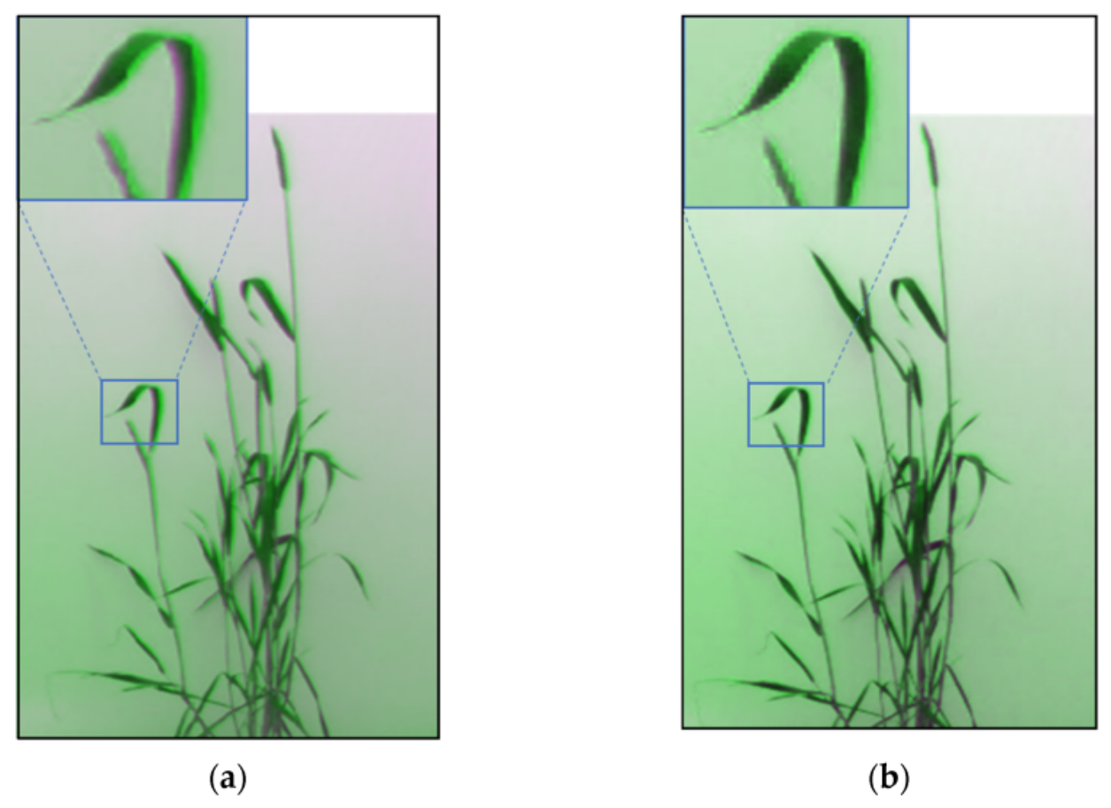
For data-level fusion, whether images from different sensors can form stable correspondences within the same spatial coordinate system directly affects subsequent feature extraction and channel combination. Sharma et al. [104] established a coarse-to-fine registration workflow for thermal infrared and optical images using greenhouse-grown wheat as the subject. As shown in Figure 3, the coarse registration results still exhibit noticeable, pink-colored misalignments at the leaf margins; following fine registration, local offsets are significantly reduced, providing a foundation for pixel-level correspondence between data from different modalities.

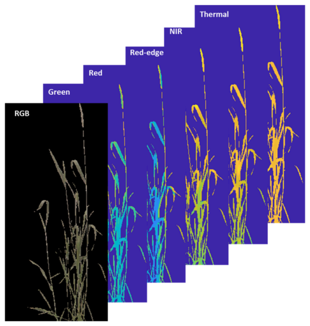
Following geometric registration, radiometric correction, and canopy segmentation, data from different sensors can be organized along the channel dimension according to the same spatial positions. Following geometric registration, radiometric correction, and canopy segmentation, data from different sensors can be organized along the channel dimension according to the same spatial positions. The data stack shown in Figure 4 contains eight channels: three broadband color channels (R, G, and B) from the RGB image, four narrowband multispectral channels (green, red, NIR, and red edge) acquired by the Parrot Sequoia multispectral sensor, and one thermal channel acquired by the FLIR T640 camera. Thus, the green and red multispectral bands are distinct from the broadband green and red channels of the RGB image. This structure preserves complementary information such as visible-light texture, near-infrared and red-edge reflectance, and canopy temperature, and can serve as a unified input for subsequent data-level fusion or multi-branch feature extraction.

Figure 3 and Figure 4 illustrate registration and construction of a pixel-aligned data stack, not direct evidence of improved disease diagnosis. Sharma et al. [104] studied greenhouse wheat phenotyping; diagnostic benefits still require unimodal baselines, ablations, and tests under misalignment or missing inputs.

Available results show why paired-data quality and validation design must be interpreted together. In one rice blast study, ground–aerial spectral fusion improved internal cross-validation by 7.36 percentage points. In the Rice-Fusion study, the multimodal model exceeded its RGB-only baseline by 13.28 percentage points. In a separate bacterial leaf blight study, accuracy decreased from 92.3% to 80.0% under cross-site and cross-year validation. These values are not directly comparable because the studies used different datasets, tasks, and validation designs. They are presented only as study-specific examples of internal and external validation evidence.

Architecture choice should match paired-sample size and task complexity. Rice- and wheat-specific studies such as RustQNet [103] and Rice-Fusion [99] provide direct examples of multi-branch fusion. More generally, dual-branch networks can encode different data types separately, while smaller datasets may favor explicit lesion, band, or vegetation-index features combined with SVM, RF, or XGBoost. These are general methodological options and are not treated here as direct evidence of performance in rice or wheat.

At field scale, wheat remote-sensing studies link field observations with UAV image measurements [63]. In rice UAV multispectral monitoring, cross-scale sample-label transfer highlights the need to quantify label-transfer error, spatial autocorrelation, and registration bias [98]. Neighborhood aggregation, feature pyramids, and graph models are general methodological strategies for linking different spatial scales and are discussed here as methodological options rather than established rice- and wheat-specific evidence.

From a general methodological perspective, trap-image counts can be combined at the decision level with weather and historical population records. This type of integration is discussed here as a general methodological option rather than as direct rice- and wheat-specific evidence. Evaluation should be stratified by density, developmental stage, and image quality.

Multiple encoders increase acquisition time, preprocessing, memory use, and latency. General model-design strategies such as shared backbones, compact spectral encoders, knowledge distillation, early exits, and confidence-triggered sensing may reduce this burden. These strategies are discussed here as general model-design options rather than as rice- and wheat-specific evidence. A hierarchical system, for example, may invoke costly modalities only for low-confidence samples; its thresholds, trigger rate, false negatives, latency, and energy use should all be reported.

In summary, fusion reliability depends on alignment, fair baselines, fault-tolerance tests, and transparent resource reporting. Existing evidence does not yet show that additional modalities consistently reduce field-survey workload or improve management outcomes.

5. Time-Series Forecasting and Early Warning of Rice and Wheat Diseases and Insect Pests

Compared with classification, detection, and segmentation, relatively few studies use continuous time series to forecast rice or wheat diseases and pests. Direct evidence includes multistage remote-sensing prediction of wheat Fusarium head blight [50], long-term seasonal forecasting of brown planthopper [105], shorter-term pest forecasting with phenology, weather, and NDVI [106], and five-day rice leaf folder forecasts [107]. These pest species are presented as representative examples rather than an exhaustive list of rice and wheat pests. This section therefore does not treat current models as mature operational warning systems. It instead examines time-series inputs, forecast windows, mechanistic and data-driven models, risk outputs, and prospective validation, while distinguishing disease-risk forecasting from population forecasting for migratory pests.

Time-series forecasting asks whether risk will rise over coming days or key growth stages, how severity will change, and how much warning time is available, rather than only identifying current symptoms. Continuous inputs, temporal features, predictive models, risk outputs, and prospective validation form the temporal modeling chain. Rice and wheat studies provide direct evidence [50]. Studies in other crops demonstrate environmental-sequence disease prediction [51] and spore-transport modeling [52]. These studies show methodological feasibility and possible transfer pathways, while aphid-monitoring research links identification to forecasting [53]. Cross-year testing and probabilistic calibration distinguish historical replication from out-of-time prediction.

5.1. Time-Series Data, Time Windows, and Prediction Models

Time-series early-warning data mainly include environmental time series, remote-sensing time series, and pest or pathogen monitoring records. They describe outbreak drivers, crop-canopy responses, and changes in pathogen or pest pressure, respectively. Because their sampling frequencies, missing-data mechanisms, and preprocessing requirements differ, they should not be concatenated into a single sequence without explicit alignment and documentation.

Environmental time series primarily comprise variables such as temperature, relative humidity, precipitation, leaf wetness, wind speed, and soil moisture, which are typically collected continuously at hourly or daily intervals by field weather stations or Internet of Things (IoT) sensors. During preprocessing, it is necessary to identify sensor anomalies and consecutive missing observations, and to construct daily averages, extreme values, cumulative precipitation, duration of continuous wetness, and lagged variables in accordance with the mechanisms underlying pest and disease occurrence. It is also necessary to standardize sensor ranges and statistical time scales across different plots or years to avoid mistaking equipment variations for changes in risk.

Remote-sensing time series consist mainly of multitemporal UAV imagery, satellite imagery, and associated vegetation indices, canopy temperature, or texture features. Sampling intervals are generally longer than those for environmental sensors and are affected by cloud cover, illumination, flight planning, and sensor configuration. Before modeling, these data require geometric registration, radiometric correction, cloud-shadow removal, and interdate normalization, while the actual acquisition dates must be retained. Missing dates should be interpolated cautiously to avoid creating canopy-change trajectories that were never observed.

Time-series data for pest or pathogen monitoring primarily include insect counts from light traps and pheromone traps, field survey records, and spore capture rates, typically recorded at daily, weekly, or fixed survey intervals. Such data are characterized by a high frequency of zero values, strong dispersion, and pronounced peaks; during preprocessing, it is necessary to standardize trapping durations and survey intensity, while recording events such as equipment replacement, pesticide application, and human intervention. Where necessary, logarithmic transformation or probability distributions suitable for count data may be applied; however, care must be taken not to eliminate genuine peaks in pest populations or spore counts through excessive smoothing.

Following the completion of quality control for the above three categories of time-series data, temporal alignment must be performed within the “field plot–date–growth stage” framework. The input time window is determined jointly by the mechanisms of pest and disease occurrence and the forecasting objectives. Wheat fusarium head blight is primarily associated with warm and humid conditions around the time of heading and flowering; rice blast involves prolonged wetness, suitable temperatures, and susceptible growth stages; while migratory pests are also linked to wind patterns and changes in pest populations. If the window is too short, cumulative effects may be overlooked, and if it is too long, information unrelated to the current risk may be included. When the prediction step size and the time of label formation are not strictly distinguished, contemporaneous identification can easily be misinterpreted as an early warning.

Early warning for migratory pests differs fundamentally from disease forecasting. Outputs should extend beyond current pest class or abundance to include future immigration abundance, peak immigration time, population density, and the probability of exceeding an economic threshold. Hu et al. used long-term light-trap records, source-region populations, and indices of the Western Pacific Subtropical High to forecast seasonal immigration of brown planthoppers into the lower Yangtze River basin [105]. Skawsang et al. integrated meteorological data, MODIS NDVI time series, and light-trap catches and showed that crop phenology improved forecasts of brown planthopper abundance [106]. Bao et al. developed a Kalman-filter model from five-day insect counts and meteorological observations at four plant protection stations from 1994 to 2014. Forward testing on 2012–2014 data yielded an overall mean accuracy of 84.33% for rice leaf folder forecasts [107]. Together, these studies show that pest early warning must account for source populations, atmospheric circulation, crop phenology, and historical abundance, and that cross-year, cross-station, and forward validation are needed to distinguish genuine forecasting from historical fit.

Once the time window has been determined, existing research primarily employs statistical learning and deep time-series models for risk modeling. Logistic regression, RF, XGBoost [78], and Bayesian models can predict the probability of occurrence using cumulative temperature and humidity within the window, the number of rainy days, and historical disease incidence; their parameters and variable contributions are relatively easy to interpret, making them suitable as baselines under conditions of limited data or few years of observation. LSTM models [51] use gating structures to capture lag effects, while Temporal CNNs employ one-dimensional convolutions to extract local variations and periodic patterns; Transformers, meanwhile, use attention mechanisms to identify key time segments. Vegetation indices, the red edge, and canopy temperature from multitemporal remote sensing data can also form time-series inputs, enabling models to simultaneously describe both growth processes and disease progression. However, in the absence of forward-looking projections or cross-year or cross-regional testing, the advantages of complex models may still stem primarily from their fit to the training data.

5.2. Mechanistic and Data-Driven Hybrid Modeling

Mechanistic models, based on the processes of pathogen infection, incubation, disease onset, and spread, convert variables such as temperature, humidity, leaf wetness, host susceptibility, and pathogen population density into infection suitability or daily risk. Compared with purely data-driven models, their advantage lies in the fact that the state variables and parameters have clear biological significance; however, model thresholds typically require recalibration according to regional climate, cultivar, and cultivation practices.

Ishiguro and Hashimoto [108] described the Yoshino leaf blast model and BLASTAM for rice blast forecasting. The Yoshino model relates infection conditions to temperature and the duration of leaf wetness. Because leaf wetness is not directly observed by the meteorological system, BLASTAM estimates the wet period from precipitation, wind speed, and sunshine duration. Rainfall is used to identify potential wet periods, while sunshine and wind conditions help determine whether the wet period continues or ends. The estimated wetness duration is then combined with temperature conditions to classify infection risk as favorable, semi-favorable, or unfavorable.

Forecasts of wheat Fusarium head blight generally use heading and flowering as temporal anchors and define risk windows from warm and humid conditions before and after flowering. De Wolf et al. [109] developed logistic-regression models from 50 location–year combinations, using rainfall duration during the 7 days before flowering, the duration of temperatures between 15 and 30 °C, and post-flowering periods with high humidity and suitable temperature as predictors. Model accuracy ranged from 62% to 85%, and four models correctly classified 84% of the location–year combinations. Their study shows that biologically defined windows around flowering can support interpretable Fusarium head blight risk equations.

Mechanistic and data-driven approaches can be combined [110]. Favorable-infection days from BLASTAM, Yoshino-based infection estimates, or a flowering-period moisture index for Fusarium head blight can serve as inputs to RF, XGBoost, or LSTM models. Alternatively, mechanistic model outputs can define prior risk and be updated with real-time sensor or remote-sensing data in a Bayesian framework. Growth-stage and infection constraints can also be incorporated into the loss function or state-transition process to prevent implausibly high risk estimates during non-susceptible periods. The purpose of hybrid modeling is not added complexity, but greater stability of data-driven models in anomalous years and unfamiliar regions.

5.3. Early-Warning Outputs, Evaluation Metrics, and Prospective Validation

Time-series models may output occurrence probability, severity trend, risk level, warning lead time, or a spatial risk map. Alongside AUC, F1, RMSE, and MAE, operational evaluation should report lead time, false alarms per unit time, and false-negative rates for high-risk events (

Table 5. Evaluation metrics for time-series early warning.

Metric	Definition	Purpose
Lead time	Alert-to-onset/threshold days	Response window
False-alarm rate	False alerts/fixed time window	Alert burden/cost
High-risk miss rate	Missed/all high-risk events	Severe-outbreak protection

). Event definitions, response windows, and decision thresholds must be fixed before testing.

Temporal independence requires chronological, cross-year, or forward splits in which only information available at the prediction time is used. Randomly splitting adjacent observations allows weather and epidemic conditions to leak across sets. Historical incidence, fixed meteorological rules, logistic regression, and univariate models provide useful time-aware baselines.

Generality is also limited by the number of epidemic years and by incomplete records of interventions. Weather stations, remote sensing, and field surveys seldom share the same frequency or coverage, while pesticide application, irrigation, or altered sowing dates can change disease trajectories. Without these records, a model may attribute management effects to natural progression.

Table 6. Representative evidence, model outputs, and application validation status for multimodal fusion and temporal prediction in rice and wheat monitoring.

Target/Ref.	Data/Validation	Method	Key Result	Output/Use	Validation
Rice blast [39]	Spectra + UAV MS; 10-fold CV; stage inconsistent	Cross-scale fusion	OA 96.37%; κ 0.95	Class/severity probabilities; affected-area check	Internal CV; management link untested
Rice diseases [99]	3200 pairs; 70:20:10 random split; stage unreported	RGB + agro-weather fusion	Accuracy 95.31%	Class + confidence; review uncertain cases	Random internal split; no application test
Rice BLB [98]	3 fields; 658 train + 120 external; stages unspecified	Label transfer + spatial–spectral fusion	OA 92.3% internal; 80.0% external	Disease-probability map; spatial check	Cross-site/year; no prospective trial
Wheat FHB [50]	2 counties; 45 field plots; 189 spectra; 1 year; heading–maturity	Temporal RS; host + weather	OA 0.71–0.93; AUC 0.66–0.75	Stage risk maps; verify flowering risk	Manual surveys; single year; no prospective trial
Rice blast [37]	Thermal + optical; canopy/leaf models; controlled early stages	Thermal–optical fusion; SVM/FPGA	Canopy OA 92%; leaf OA 97%; 72 h early; FPGA 92%	Early class; edge recheck trigger	Controlled study; no external or forward field trial
Wheat FHB [71]	50 plots × 2 dates; 100 samples; 80:20 split; 5-fold CV; filling stage	UAV-HS spectral + texture + color; RF	Prediction 85%; 5-fold CV 83%	3 severity classes + map; field check	One field/year; random split; no management trial
BPH [105]	Multiyear traps, source counts, circulation indices; stages/migration periods	Source/ circulation forecast	Seasonal abundance and peak timing predicted	Abundance + peak timing; regional warning	Multiyear series; management effect untested
BPH [106]	2006–2016 traps, weather, MODIS NDVI; dry season	ANN/RF/MLR forecast	RMSE 1.686 (ANN), 1.737 (RF), 2.015 (MLR)	Abundance + peak timing; pest warning	Holdout; no region transfer or management test
Rice leaf folder [107]	4 stations; 5-day counts + weather, 1994–2014; migration/damage periods	5-day Kalman forecast	Operational accuracy 84.33% (2012–2014)	Next-5-day abundance; station warning	Out-of-time trial; no region transfer or management test
Rice blast [111]	94 fields, 2021–2024; train 2021–2023/test 2024; 35/55 DAS	Sentinel-2; KNN, RF, SVM	RF at 55 DAS: accuracy 0.94; F1 0.91; specificity 0.96	Field infection class; targeted scouting	Independent year; one region; one variety; management effect untested

Note: BLB, bacterial leaf blight; FHB, Fusarium head blight; BPH, brown planthopper; MS, multispectral; RS, remote sensing.

separates multimodal classification outputs from temporal risk outputs. Table 6 presents study-specific examples of multimodal fusion and temporal prediction performance under different validation settings. Because these studies differ in datasets, tasks, and validation designs, the reported values should not be interpreted as directly comparable effects. For example, the wheat Fusarium head blight study produced stage-specific risk maps (OA 0.71–0.93; AUC 0.66–0.75) but covered only 45 plots in one epidemic year. These outputs may support field verification, but their management benefits have not yet been prospectively validated.

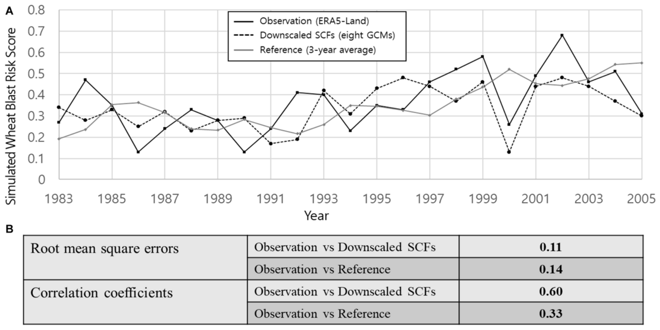
Historical hindcasting provides a retrospective assessment of temporal predictability, but it does not substitute for independent-year or prospective validation. Kim and Choi [112] evaluated seasonal wheat-blast risk over the common 1983–2005 hindcast period using ERA5-Land, downscaled seasonal forecasts from eight global climate models, and a three-year historical-mean reference. The forecast-driven simulations reduced RMSE from 0.14 to 0.11 and increased the temporal correlation coefficient from 0.33 to 0.60 relative to the reference. Figure 5 is retained as a methodological example of retrospective hindcast evaluation rather than as recent operational-validation evidence.

More recent rice-blast studies have used updated observations, although their validation strength has varied. Gopalakrishnan et al. [113] modeled weekly disease incidence and meteorological records collected at three locations during 2015–2023. The ANNX model achieved a lower test RMSE (5.01) than SVRX (5.84) and INGARCHX (6.99); however, the 80:20 holdout remained an internal evaluation rather than an independent-year test. In contrast, Agenjos-Moreno et al. [111] used data from 2021–2023 for model development and reserved the 2024 growing season for independent validation. Based on Sentinel-2 observations from 94 fields, the RF model achieved a validation accuracy of 0.94, an F1-score of 0.91, and a specificity of 0.96 at 55 days after sowing. These findings show that retrospective hindcasting, internal holdout testing, and independent-year validation should be reported separately because they support different levels of temporal generalization evidence.

Because the same predicted risk can correspond to different incidence rates across years or regions, early-warning probabilities should be calibrated on an independent set. Temperature scaling is a simple post hoc method [114]. Reports should pair calibration error with recall and false-alarm counts across decision thresholds, including low- and high-incidence years.

In prospective trials, the model and thresholds are frozen before the growing season, predictions are generated from newly available data, and prediction times, surveys, incidence, missing observations, and interventions are recorded. This design provides stronger evidence of temporal independence than retrospective replay but remains rare in rice and wheat research.

6. Field Robustness and Generalization: Validation Frameworks and Reporting Standards

This section shifts from model architecture to the strength of generalization evidence. Field data do not by themselves demonstrate field generalization: when training and test samples share a field, year, cultivar, or device, a model may exploit background or acquisition cues that will not persist elsewhere.

The proposed sequence is as follows: define source and target domains, enforce sample independence, conduct stress tests, perform external validation, and assess uncertainty.

Table 7. Field-generalization validation matrix for rice and wheat disease and pest models.

Validation Type	Recommended Design	Report	Supports
Object independence	Group at the highest hierarchical level required to isolate correlated observations (e.g., source image, leaf, plant, field, or UAV mission)	Grouping unit; independent objects per split	Same-source object-level performance
Spatial external	Leave-one-location/field-out	Site differences, sample sizes, performance loss	Cross-site transfer
Temporal external	Leave-one-year-out or forward chaining	Train/test years; climate differences	Cross-year transfer
Biological external	Leave-one-cultivar/stage-out	Cultivars, stages, symptom severity	Cross-cultivar/stage transfer
Device external	Leave-one-camera/UAV/spectrometer-out	Device specs; calibration	Cross-device transfer
Robustness stress	Vary light, occlusion, noise, alignment, missing modalities	Perturbation level; worst-group result	Robustness to stated perturbations
Trustworthy output	Calibration, OOD detection, rejection testing	ECE, OOD rate, rejection rate	Confidence reliability/anomaly detection
Prospective	Freeze model pre-season; test on new data	Prediction time, surveys, interventions	Temporal independence + operational feasibility

specifies the conclusions supported by each validation design.

6.1. Validation-Domain Definition, Sample Partitioning, and Data-Leakage Control

The source domain comprises the plots, years, cultivars, devices, and acquisition conditions used for development; the target domain comprises intended conditions excluded from training. Reporting which environmental, biological, spatial, temporal, or equipment factors change distinguishes internal, single-factor external, and multi-factor cross-domain tests.

Different validation designs assess different aspects of model generalization. Random internal splitting and object-grouped testing assess within-domain performance and sample independence. External validation assesses transfer across changes in site, year, cultivar, or device. Prospective validation assesses performance on future data with a fixed model. These designs are complementary rather than strictly hierarchical. External metrics should be reported with the decline from internal performance and its confidence interval.

Samples should be partitioned at the highest hierarchical level required to isolate correlated observations, such as the source image, leaf, plant, field, or UAV mission. All observations and modalities from one object must remain in one subset. Normalization, imputation, feature selection, and augmentation must be fitted on training data only; otherwise, duplicate objects, spatial proximity, or preprocessing can leak test information.

6.2. Comparison of Robustness Stress Testing and Data Augmentation Methods

Robustness methods should be compared on a fixed independent test set. Starting from one baseline, add augmentation, transfer learning, domain adaptation, modality pruning, or quality gating while holding the data, metrics, and random seeds constant. Augmentation and adaptation cannot repair leakage in the original split.

Stress tests should target predefined shifts: illumination, blur, occlusion, background, and distance for RGB; noise, misregistration, and device drift for spectral or thermal data; and missing or degraded inputs for multimodal systems. Report the performance drop, worst subgroup, high-risk recall, and calibration error rather than average accuracy alone.

Domain adaptation uses target-domain data during model adjustment; domain generalization does not. Adaptation therefore requires a non-adapted baseline, an adapted model, and a fixed target test set. Generalization requires a held-out site, year, or device and prohibits target-domain tuning of either the model or thresholds.

Models that output risk probabilities or trigger reinspection should use an independent calibration set; temperature scaling is one established method [114]. Generative models can ease data scarcity but face external generalization challenges [115]. OOD detection can reject unfamiliar cultivars, devices, backgrounds, or classes [116]. Grad-CAM and key-band attribution [10] can diagnose spurious focus but cannot replace external validation. Relevant measures include expected calibration error, rejection rate, out-of-distribution detection rate, and risk–coverage curves.

6.3. External Validation, Trustworthy Outputs and Reproducible Reports

Reproducible reports should specify data sources, sample units, grouping variables, split lists, preprocessing, model versions, thresholds, calibration and unknown class sets, random seeds, and hardware. Report class- and subgroup-level results, internal-to-external performance loss, confidence intervals, calibration error, and false rejection rates.

Under this framework, an “external test” is not automatically strong evidence; its value depends on independence in location, year, cultivar, equipment, and background. Table 4 shows that the rice multi-disease classifier exceeded 99% accuracy internally but declined to 91% on external images from different locations and years [80]. The bacterial leaf blight model declined from 92.3% to 80.0% across locations, years, and cultivars [98], whereas GDFC-YOLO retained a high mAP on external field images acquired under conditions similar to those of the development set [87]. External tests therefore differ in evidential strength according to which factors actually change between the source and target domains.

Table 7 summarizes the partitioning methods, minimum reporting items, and inferential limits of object-independent, spatial, temporal, biological, equipment, perturbation, and prospective validation.

Accuracy and confidence can fail together under domain shift. The following example is not specific to rice or wheat. It is included here as general methodological evidence of confidence miscalibration under domain shift. Xiang et al. [116] trained on the controlled PlantVillage domain and tested on field images from PlantDoc. ResNet-50 accuracy fell from 99.73% to 32.05%, although mean target-domain confidence remained 79.76%. Source-only temperature scaling reduced target ECE from 0.4771 to 0.4400; a parent-image-grouped field calibration subset reduced it to 0.3651, with substantial overconfidence remaining (Figure 6). External tests should therefore report both discrimination and calibration under clearly defined sample grouping.

Current external tests usually vary only one site, year, or device. Multi-factor tests should jointly consider location, year, cultivar, growth stage, equipment, illumination, symptom severity, and occlusion. Performance loss is itself evidence of a model’s scope; analyses should identify affected classes and worst subgroups, changes in calibration, and recovery after robustness enhancement.

7. Current Challenges and Future Directions

The evidence reviewed above suggests several research priorities. These priorities are organized according to current evidence gaps and implementation needs rather than fixed time horizons. The first group focuses on data quality, evaluation, and deployment. The second group focuses on cross-domain generalization, integrated systems, and prospective field validation.

7.1. Priorities for Data, Evaluation, and Deployment

External performance losses across locations and years have been reported for multiclass rice-disease diagnosis [80] and UAV bacterial leaf blight mapping [98]. Existing data should therefore be reorganized by plot, date, growth stage, and device, with metadata for cultivar, symptom stage, acquisition conditions, and management. Standard splits and baselines should include weak symptoms, combined and non-disease stresses, occlusions, and true negatives. Class-wise recall, failed samples, annotation agreement, and tuning ranges should be reported. Self-supervised, semi-supervised, weakly supervised, and active learning can reduce annotation cost while retaining an expert-reviewed subset.

RGB–agrometeorological rice-disease fusion demonstrates the benefit of complementary modalities [99]. Multimodal studies should improve alignment and quality-aware gating, then compare single-, partial-, full-, missing-, and misaligned-modality conditions on the same test set. Multistage Fusarium head blight prediction shows the value of biologically defined windows [50]. Time-series work should use forward splits and report lead time and false alarms. Mechanistic priors, such as favorable infection days or flowering-stage moisture, can first be introduced as features but require multiyear calibration.

Photothermal rice-blast sensing demonstrates FPGA edge inference [37], and embedded wheat-rust classification demonstrates device-level deployment [85]. Evaluations of plant-disease mobile apps also reveal practical quality limits [117]. Deployment studies should standardize input size, parameter count, memory, latency, energy use, offline operation, and cross-device performance. Mobile and embedded systems should implement a predefined “model output–manual review–result correction” loop and report false positives per unit time, high-risk false negatives, rejection rates, and reviewer workload.

7.2. Priorities for Cross-Domain Generalization and Prospective Validation

Long-term datasets should span regions, years, cultivars, and devices while linking RGB, spectral, thermal, environmental, pest or spore, and management records within the same plots. Labels should cover growth stage, progression, severity, combined stress, and outcomes. Hybrid models can then represent the sequence from environmental drivers and host response to pathogen or pest dynamics and symptoms. Generative models can augment scarce agricultural training data, while emerging vision–language approaches may support multimodal agricultural analysis [115]. These methods may be useful when labeled crop-disease or pest data are limited. However, their practical value still requires crop-specific and cross-domain validation under different cultivars, growth stages, locations, and devices.

A cloud–edge–device architecture [118] could connect field sensors, mobile devices, UAVs, and machinery [119]. Existing IoT–UAV [120] and detection–mixing–spraying systems [121] show technical feasibility, but communication reliability, maintenance, model drift, updating, and rollback remain unresolved. Cross-season prospective trials should freeze models in advance and record predictions, surveys, actions, follow-up severity, inputs, and economic outcomes. Importantly, high classification or prediction accuracy does not necessarily indicate agronomic benefit. Model accuracy should therefore be regarded as a technical outcome rather than direct evidence of practical value. Future prospective studies should compare model-assisted management with conventional field scouting or standard practice. They should evaluate whether model use can reduce pesticide inputs, improve disease or pest control, limit yield loss, and provide measurable economic benefits. Most available cost estimates are based on studies in developed countries. Actual costs may differ across regions because equipment prices, labor costs, maintenance, and technical support vary. Therefore, regional conditions should be considered when evaluating economic feasibility.

For migratory pests, longer-term systems must connect immigration, colonization, population growth, and damage. Long-term brown-planthopper forecasting links source populations and atmospheric circulation [105]. Short-term population models add crop phenology, weather, and satellite NDVI [106]. Five-day rice-leaf-folder forecasting combines insect counts with meteorology [107]. These inputs should support forecasts of peak timing, density, and economic-threshold exceedance. Cross-site and cross-year forward trials are essential.

8. Conclusions

Intelligent monitoring of rice and wheat diseases and insect pests now spans classification, detection, segmentation, multimodal fusion, and time-series forecasting. Across seedling, tillering/jointing, heading/flowering, and grain filling/maturity stages, environmental and physiological signals support risk forecasting, visible symptoms support identification, and affected area or pest density supports severity estimation. Evidence is uneven across diseases, insect pests, growth stages, and validation types. The representative literature reviewed here suggests greater research attention to the tillering/jointing and heading/flowering stages; however, this observation is qualitative because growth-stage information is not consistently reported across studies. Evidence is still limited for presymptomatic seedling monitoring, disease–senescence discrimination at grain filling/maturity, and cross-stage stability. These conclusions are based on a qualitative synthesis of representative studies. They do not represent a formal quantitative comparison.

A major limitation is the strong reliance of public and benchmark datasets on RGB imagery. RGB data are useful for low-cost recognition and localization of visible disease symptoms and insect pests. However, models trained only on RGB datasets may face challenges in generalizing to heterogeneous field conditions and may provide limited support for presymptomatic early warning and operational decision-making. Future datasets should therefore integrate RGB data with spectral, thermal, environmental, and temporal information and include multisite and multiyear field observations.

Unimodal methods remain essential baselines: conventional machine learning is useful for smaller, interpretable datasets, whereas deep learning supports complex visual representation and localization. Multimodal and temporal models add complementary evidence only when alignment, sample independence, and prediction timing are controlled.

Reliable performance across new fields, seasons, cultivars, devices, and operating conditions remains a major challenge. Future studies should place more emphasis on independent validation. They should also improve calibration, reproducibility, and field evaluation.