Improved YOLOv8 Weed Segmentation Method Based on Dual-ViT

Abstract

To address inaccurate weed segmentation under crop overlap, occlusion, and complex field backgrounds, this study developed a combined method integrating DViT-YOLOv8-seg with confidence-guided SLIC voting. The dataset contained 1872 field images (800 × 600 pixels) of Guangzhou soft-stem lettuce and four common weed species: Eleusine indica, Digitaria sanguinalis, Portulaca oleracea, and Amaranthus blitum. All weed species were merged into one weed class, while lettuce, soil, and other field regions were treated as non-weed. Real-ESRGAN and data augmentation enhanced the training samples; Dual-ViT strengthened global–local feature interaction; GSConv reduced redundant computation; BiFPN improved multi-scale fusion; and SLIC refined ambiguous boundaries. After super-resolution preprocessing and three-fold expansion, baseline mPA increased by 10.9 percentage points. The improved network achieved 88.3% mPA at 7.9 GFLOPs, corresponding to +3.6 percentage points and -1.0 GFLOPs relative to the baseline. SLIC voting increased FWIoU to 95.6%, 4.1 percentage points above the network without SLIC. Compared with YOLOv5-seg and Fast-SCNN, mPA improved by 2.0 and 6.5 percentage points, respectively; GFLOPs were 87.7% and 95.5% lower than those of YOLOv5-seg and DeepLabv3+, respectively. The method therefore provides a favorable trade-off between segmentation accuracy and theoretical network computation for complex lettuce field imagery.

1. Introduction

Farmland weeds are common hazards in agricultural production. With strong reproductive capacity, weeds compete for nutrients, spread diseases, and attract pests, thereby reducing crop yield and quality and causing agricultural economic losses. In recent years, the promotion of smart agriculture has gradually driven weeding toward intellectualization and automation. Numerous studies have adopted visual [1,2,3], tactile [4,5], and visual–tactile fusion methods [6,7,8] for weed detection. Among relevant technologies, image processing has become one of the important means for farmland condition perception. Many scholars have adopted object detection methods to obtain field weed information. However, due to the diverse morphologies and easy deformation of weeds, densely overlapping bounding boxes often occur for scatter-shaped weeds, making detection information difficult to use effectively. To overcome this drawback, numerous researchers have employed image segmentation for weed information perception.

Miao et al. [9] realized weed recognition by fusing multiple features including color, texture, and fractal box dimension of crops and weeds, achieving an average recognition rate of 83.78%. Zhang et al. [10] proposed a method combining the adaptive fuzzy dynamic K-means algorithm, optimized GrabCut algorithm, and SRC (sparse representation-based classification algorithm), which enabled automatic weed segmentation from the background without manual intervention. Although traditional image processing methods based on artificially designed features and parameters have achieved certain effects in weed detection and segmentation, the designed features and parameters can hardly represent natural characteristics when dealing with complex lighting, complex background interference, and overlapping occlusion between crops and weeds, resulting in a significant decrease in segmentation accuracy. In contrast, deep learning can automatically learn hierarchical features in images, effectively extract useful information from complex backgrounds, and exhibit superior performance in handling complex field environments. Osorio et al. [11] used SVM-HOG, YOLOv3, and Mask R-CNN combined with multispectral images to identify lettuce. The detected crops were converted into binary masks and fused with an NDVI background subtractor to indirectly obtain weed images. The F1 scores of the three algorithms were 88%, 94%, and 94%, respectively. Hu et al. [12] proposed a lightweight Multimodule-YOLOv7-L model for real-time localization of lettuce and weeds and classification of in-row weed severity; the model achieved a precision of 97.5% and a recall of 95.7%. Sun et al. [13] employed YOLOX and Deformable DETR models, to detect pak choi seedlings, among which YOLOX achieved an average precision of 98.1% and a detection speed of 44.8 fps, demonstrating favorable real-time performance. Jin et al. [14] utilized DenseNet, RegNet, and ShuffleNet classification networks to identify pak choi in grid-based images, and subsequently combined color segmentation to distinguish weeds from soil. ShuffleNet required only 14.12 ms per image, achieving an overall accuracy exceeding 96.5%. Wang et al. [15] proposed a corn segmentation method based on a Swin Transformer. Based on corn morphological segmentation, an optimized combined algorithm of image morphological processing was constructed to realize weed segmentation under overlapping occlusion between crops and weeds. Abdalla et al. [16] presented a rapeseed segmentation method that combines SVM and an improved encoder of the SegNet network, achieving precise segmentation of lettuce in the presence of dense weeds with a maximum accuracy of up to 96%. Cai et al. [17] developed a semi-supervised Chinese flowering cabbage weed segmentation method based on UANP-MT, achieving a pixel accuracy of 95.84%.

In summary, deep learning-based methods have substantially improved crop–weed recognition, but the reported overall accuracies do not fully resolve the coupled difficulties encountered in lettuce fields. Detection- and classification-based approaches provide limited pixel boundary information; conventional CNN segmentation can lose long-range context during repeated downsampling; and high-capacity networks or external post-processing may improve masks without demonstrating a balanced end-to-end computational cost. These weaknesses become more pronounced when broadleaf weeds resemble lettuce leaves, small weeds occupy few pixels, illumination changes reduce local contrast, and crop–weed occlusion disrupts object continuity. Therefore, accurate field segmentation requires the simultaneous preservation of global context, local boundary detail, and controlled network complexity rather than optimization of a single aggregate metric. This study does not claim Real-ESRGAN, Dual-ViT, GSConv, BiFPN, or SLIC as newly invented basic modules. Its methodological contribution is a task-specific DViT-YOLOv8-seg architecture together with a reproducible confidence-guided superpixel decision rule that coordinates global–local representation, weighted multi-scale fusion, and boundary correction for binary crop–weed segmentation.

2. Materials and Methods

Section 2.1 and Section 2.2 describe the experimental materials, including the image acquisition equipment and the lettuce field dataset. Section 2.3, Section 2.4, Section 2.5, Section 2.6 and Section 2.7 describe the research methods, including the overall workflow, data preprocessing, network construction, the assembled segmentation model, and the superpixel voting mechanism.

2.1. Lettuce Image Acquisition Equipment

The imaging quality of raw field images directly affects the extraction of lettuce and weed features. A Hikvision MV-CA013-20GC CMOS industrial camera, manufactured by Hangzhou Hikvision Digital Technology Co., Ltd., Hangzhou, Zhejiang, China, was used as the image acquisition device. Raw images were recorded at 800 × 600 pixels and stored in JPG format. Exposure, gain, and white balance settings were kept fixed during each acquisition session to reduce imaging variation caused by automatic camera adjustment.

The camera was mounted vertically on an adjustable metal support, with the lens positioned 1.2 m above the field surface. Images were captured at approximately 0.3 m intervals along the lettuce ridges to improve coverage of inter-row scenes and variations in crop–weed overlap.

2.2. Lettuce Image Dataset

Field image collection and model recognition performance verification experiments were carried out at the Agricultural Experimental Base of South China Agricultural University in November 2025, with raw data collected from October to November 2025. The dataset used for model training and testing consists of 1872 field lettuce images, which were randomly split into training, validation, and test sets at a ratio of 7:2:1.

The experimental crop is a local lettuce cultivar widely grown in Guangzhou—Guangzhou soft-stem lettuce. Images were collected when lettuce was at the early-to-middle rosette stage, 18–26 days after transplanting, with each plant bearing 5–7 leaves and a plant height ranging from 10 to 15 cm. The leaves of this lettuce cultivar heavily overlap with weeds, and broadleaf weeds share highly similar morphological features with lettuce foliage, creating the most challenging visual recognition scenarios for field weeding tasks.

The co-occurring weeds comprised four dominant seedling species commonly found in South China vegetable fields. All weeds were at the seedling stage, approximately 5–12 days after emergence and 2–8 cm in height, including two grass species, Eleusine indica and Digitaria sanguinalis, and two broadleaf species, Portulaca oleracea and Amaranthus blitum. Grass weeds have narrow elongated leaves, whereas the broadleaf weeds are more similar to lettuce foliage and are frequently occluded by crop leaves. For model training and evaluation, the four weed species were merged into a single weed class; lettuce, soil, residues, and other field regions were assigned to the non-weed class. This binary definition matches the operational requirement of distinguishing treatment targets from protected crop and background regions.

Images were collected during sunny morning and afternoon periods and supplemented with samples under weak overcast light, backlighting, tree shade, and crop leaf occlusion. These acquisition conditions increased the diversity of illumination and overlap represented in the dataset without implying complete coverage of all field environments.

2.3. Overall Workflow of the Segmentation Method

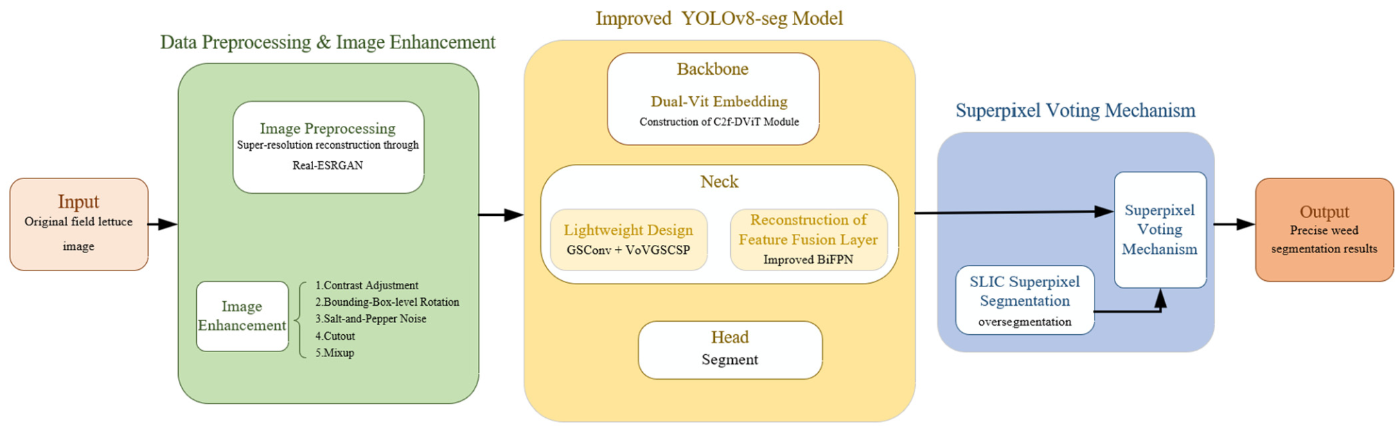
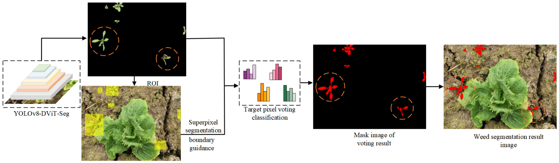
The proposed method comprises a continuous sequence from field image acquisition and input to the final weed mask. Raw images undergo Real-ESRGAN preprocessing and data augmentation, followed by initial segmentation using the improved DViT-YOLOv8-seg network. The resulting probability map is then combined with the SLIC superpixel partition for boundary correction. Figure 1 therefore presents the complete pipeline from image acquisition and preprocessing, through network inference, to confidence-guided SLIC voting and final pixel-level output; the individual stages are described in the following sections.

2.4. Data Preprocessing and Image Enhancement

This section introduces the data preprocessing and image enhancement for weed segmentation. To enhance image detail and improve model generalization under complex field conditions, super-resolution reconstruction and multiple image enhancement methods are employed. The super-resolution preprocessing is described in Section 2.4.1. The image enhancement methods are described in Section 2.4.2.

2.4.1. Image Preprocessing

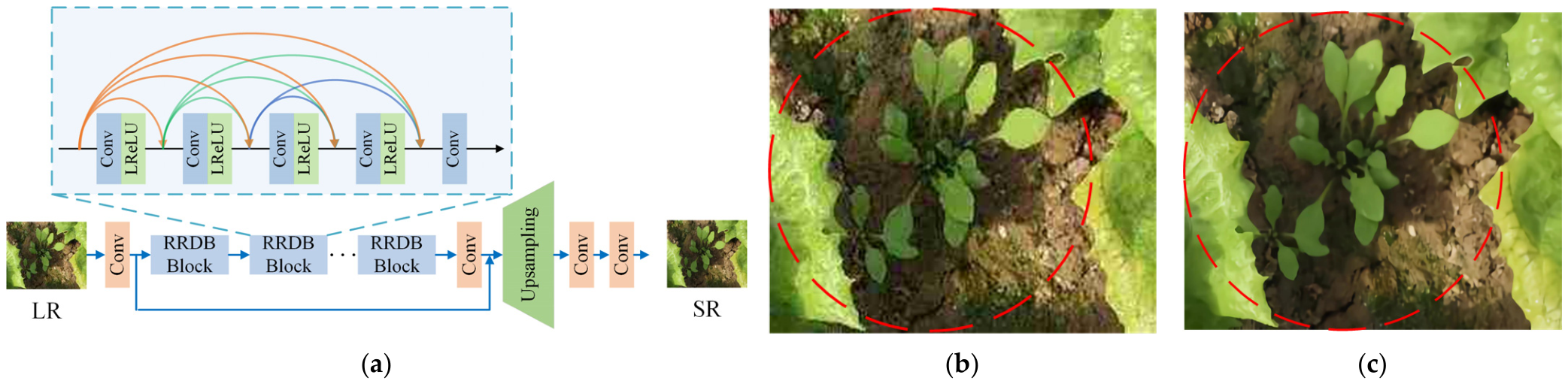
Lighting variation, background interference, and image noise can weaken weed texture and boundary information. To improve the visibility of fine structures, a pretrained Real-ESRGAN model was used for super-resolution preprocessing [18,19,20]. Real-ESRGAN is an ESRGAN-derived blind super-resolution framework whose RRDB-based generator reconstructs high-frequency details from degraded inputs. The architecture is summarized in Figure 2a [21], and a representative local result is shown in Figure 2b,c; detailed implementation characteristics are available in the cited studies.

2.4.2. Image Enhancement

To enhance the model’s learning ability for edge detection, random contrast adjustment was applied to the images. To improve the anti-interference capability of the model, bounding box-level salt-and-pepper noise was introduced. To simulate the mutual occlusion between crops, bounding box-level rotation was employed. The Mixup technique was used to mix two random images at a certain ratio. In addition, the Cutout method was adopted to remove partial content of images. The effects of each data augmentation method are shown in Figure 3.

Contrast adjustment was used to simulate illumination variation and improve exposure diversity. Salt-and-pepper noise was intended to mimic localized sensor or field contamination. Bounding box-level rotation increased target pose diversity. Cutout reproduced partial occlusion by crop leaves, and Mixup increased the frequency of overlapping crop–weed patterns while reducing reliance on individual backgrounds. These augmentations were applied jointly; their individual causal effects were not inferred from the combined preprocessing experiment.

2.5. Construction of the Weed Segmentation Method

This section introduces the construction of the improved weed segmentation network based on YOLOv8-seg. Aiming at the problems of insufficient global feature extraction ability, excessive computational redundancy, and weak multi-scale feature fusion in the original model, a multi-module collaborative improvement strategy is proposed. The embedding of the Dual-ViT backbone into the feature extraction network is described in Section 2.5.1. The lightweight of the neck network is described in Section 2.5.2. The reconstruction of the feature fusion layer is described in Section 2.5.3.

2.5.1. Embedding of the Dual-ViT Backbone

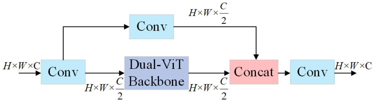
Convolutional neural networks suffer from the loss of long-range dependencies caused by continuous downsampling, making it difficult to capture global information and thus limiting segmentation accuracy [22]. Meanwhile, higher requirements are placed on local pixel-level feature extraction to achieve accurate boundary segmentation of mutually occluded targets under complex backgrounds. The Transformer architecture realizes attention focusing similar to biological vision via MHSA (multi-head self-attention), which can effectively extract contextual information of focused targets and well suppress interference from complex backgrounds and mutual occlusion [23,24]. In this paper, the backbone of dual-vision Transformer is embedded into the first C2f module of the feature extraction network to construct the C2f-DViT module [25], whose structure is shown in Figure 4.

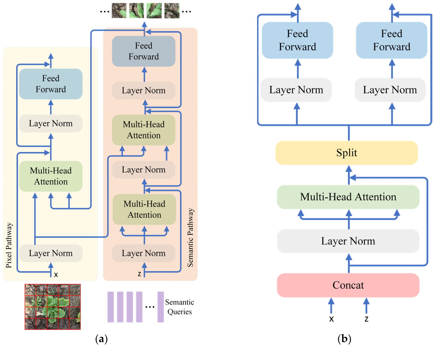
The DViT backbone consists of two components: a dual block (Figure 5a) and a merge block (Figure 5b). The dual block is composed of two branches, namely the semantic branch and the pixel branch. The semantic branch can effectively compress token vectors into global semantics, which can serve as useful prior information for the pixel branch to learn finer local pixel details. Guided by the global semantic prior, the pixel branch employs multi-head attention to implement cross-attention, thereby capturing fine-grained information while refining input features at the pixel level. The semantic branch and pixel branch are combined and jointly trained to propagate the enhanced self-attention information in parallel through the two branches.

Given the input feature of the dual block as x_l, the semantic branch first encodes global semantics contextually through self-attention, then applies cross-attention to interact between the refined global semantics and the input feature x_l to extract semantic information. This semantic information is fed into the pixel branch as prior information of high-level semantics. In the pixel branch, the semantic information interacts with the input feature x_l, and the input feature is refined via cross-attention. Thus, the dual block can compensate for information loss caused by global feature compression through pixel-to-semantic interaction, and reduce the difficulty of extracting finer local features with global prior information through semantic-to-pixel interaction. The detailed process of the semantic branch is shown in Equations (1)–(4), and that of the pixel branch is shown in Equations (5)–(7).

$$x_l^n=LN\left(x_l\right),z_l^n=LN\left(z_l\right)$$

(1)

$$z_l^{\prime }=MHA(z_l^n,z_l^n,z_l^n)+z_l$$

(2)

$${\tilde{z}}_l=MHA\left(LN\right(z_l^{\prime }),x_l^n,x_l^n)+z_l^{\prime }$$

(3)

$$z_{(l+1)}=FFN\left(LN\right({\tilde{z}}_l\left)\right)+{\tilde{z}}_l$$

(4)

$$x_l^n=LN\left(x_l\right),z_{(l+1)}^n=LN\left(z_{(l+1)}\right)$$

(5)

$$x_l^{\prime }=MHA(x_l^n,z_{(l+1)}^n,z_{(l+1)}^n)+x_l$$

(6)

$$x_{(l+1)}=FFN\left(LN\right(x_l^{\prime }\left)\right)+x_l^{\prime }$$

(7)

To enable sufficient interaction of local features within the pixel branch, in the merge block, the global semantics and local features output by the dual block are merged, and self-attention is further applied to achieve internal interaction across local features. Since the semantic branch and pixel branch convey information at different scales, two separate feed-forward layers are adopted for the two branches, and the final output is generated through global average pooling. The detailed process is shown in Equations (8)–(11).

$$y_l^n=LN\left(\right[x_l\left|\right|z_l\left]\right)$$

(8)

$$x_l^{\prime },z_l^{\prime }=MHA(y_l^n,y_l^n,y_l^n)+\left[x_l\right|\left|z_l\right]$$

(9)

$$x_{(l+1)}=FF{N}^X\left(LN\right(x_l^{\prime }\left)\right)+x_l^{\prime }$$

(10)

$$z_{(l+1)}=FF{N}^Z\left(LN\right(z_l^{\prime }\left)\right)+z_l^{\prime }$$

(11)

2.5.2. Lightweight of the Neck Network

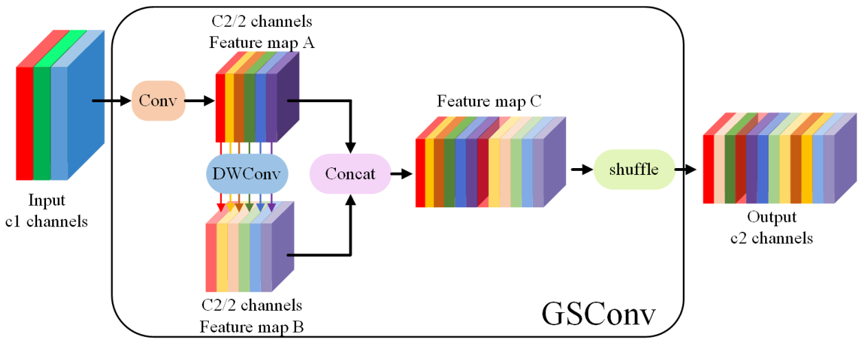
To address the unnecessary computational redundancy caused by standard convolution performing dense computation on every input channel and spatial location in the neck network [26], the GSConv module is introduced to replace the original standard convolution, making the model more compact [27]. Its structure is shown in Figure 6.

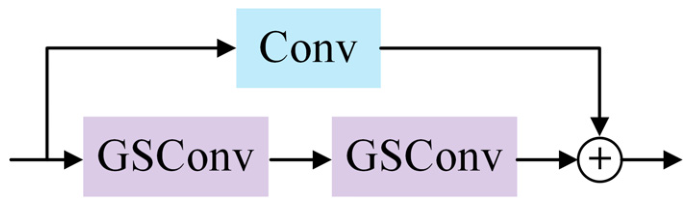
GSConv first obtains feature map A via standard convolution, then generates feature map B using depthwise separable convolution. The two sets of features are concatenated and followed by channel shuffling, enabling the full exchange of information extracted by standard convolution across different channels. For a single convolution module with equal scale, GSConv maintains relatively complete feature representation at a lower theoretical computational cost. Furthermore, this paper constructs the GS bottleneck based on GSConv (as shown in the Figure 7) and designs the VoV-GSCSP module with a one-time aggregation strategy to facilitate feature fusion at different stages (as shown in Figure 8). It should be emphasized that this computational advantage applies only to GSConv and its corresponding neck subnetwork, and cannot be directly extrapolated to a reduction in end-to-end computational complexity for the entire combined pipeline.

The standard convolutions in the PAN neck are replaced with GSConv, and the C2f modules are substituted with VoVGSCSP. This reduces the computational complexity of the model while enabling effective information fusion among feature maps at different stages, thus ensuring the model accuracy.

2.5.3. Reconstruction of the Feature Fusion Layer

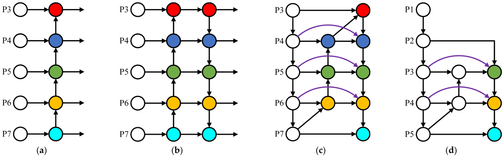
Due to the complex background, mutual occlusion, and large target scale variations in field environments [28,29], the selection of the neck network plays a crucial role in the fusion of multi-scale features. Reconstructing the feature fusion layer can improve the model’s segmentation performance for small targets and boundaries. The PAN adopted in YOLOv8 is improved from FPN (Figure 9a), and its structure is illustrated in Figure 9b. FPN adopts a top-down feature fusion strategy. Although the fused features contain more high-level semantic information, low-level semantic information is lost to a certain extent due to the restriction of unidirectional information flow, which is detrimental to the extraction of local detailed features [30]. Based on FPN, PAN adds an extra bottom-up path, which enables the high-level semantic information from deep feature layers to be transferred to shallow layers, and simultaneously transmits the low-level semantic information containing detailed features from shallow layers to deep layers, thus realizing bidirectional fusion of cross-scale features. Although PAN can achieve bidirectional fusion across feature layers, its fusion method merely performs the simple superposition of feature layers at different scales. However, simple superposition cannot distinguish the importance of input feature layers at different scales to the fused output features, which is detrimental to the extraction of target texture features under complex backgrounds. To address this issue, the improved weighted BiFPN (bidirectional feature pyramid network) is employed to reconstruct the neck network of YOLOv8 [31]. For the fusion of features with different resolutions, BiFPN assigns additional weights to each input feature, allowing the network to distinguish the importance of different features. On the basis of the original BiFPN (Figure 9c), the one-sided input nodes with low contribution rates to the feature fusion network are removed to simplify the network. Meanwhile, the large-scale feature layer P2 is added to fully utilize the abundant detailed features from shallow layers, enhancing the network’s ability to fuse texture features. An extra path is added between the input and output nodes at the same level to obtain more cross-scale feature fusion at the lowest computational cost. The improved BiFPN is shown in Figure 9d.

2.6. Improved YOLOv8-seg Model

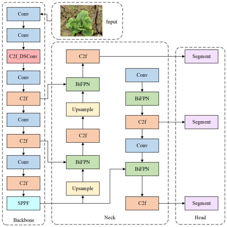
The YOLOv8-seg model is modified via the embedding of the Dual-ViT backbone, the lightweight design of the neck network, and the reconstruction of the feature fusion layer. The structure of the constructed improved YOLOv8-seg network model (DViT-YOLOv8-Seg) is illustrated in Figure 10.

The location and purpose of each architectural modification are summarized in

Table 1. Summary of model modifications and their purposes.

Modification	Position	Purpose
C2f-DViT	Backbone	Strengthen interaction between global semantics and local pixel details
GSConv + VoVGSCSP	Neck	Reduce redundant convolution while retaining cross-channel feature exchange
Improved BiFPN with P2	Neck	Apply weighted multi-scale fusion and preserve shallow details for small targets
SLIC voting	Post-processing	Correct ambiguous boundary pixels using local color and texture consistency

. A standardized configuration proposed for reproducible re-training and independent verification is provided in

Table 2. Proposed standardized training and inference hyperparameters for reproducible re-training.

Proposed Hyperparameter	Standardized Setting for Reproducible Re-Training
Model initialization	YOLOv8n-seg initialized from COCO-pretrained weights
Network input	640 × 640 pixels; aspect ratio preserved by letterbox padding
Dataset split	Training/validation/test = 7:2:1
Training duration	Maximum 200 epochs; early stopping patience = 50 epochs
Batch and loading	Batch size = 8; data loader workers = 8
Optimizer	AdamW
Learning rate	Initial learning rate = 0.001; final learning rate factor = 0.01
Regularization and schedule	Weight decay = 0.0005; cosine annealing schedule; warm-up = 3 epochs
Reproducibility and precision	Random seed = 42; automatic mixed precision enabled
Model selection	Checkpoint with the highest validation mIoU
Inference settings	Confidence threshold = 0.25; NMS IoU threshold = 0.70
Mask settings	Overlapping mask processing enabled; mask downsampling ratio = 4
SLIC settings	n_segments = 500; compactness = 10; sigma = 1.0; maximum iterations = 10
Voting settings	Pixel decision threshold = 0.50; superpixel majority threshold = 0.50

.

2.7. Superpixel Voting Mechanism

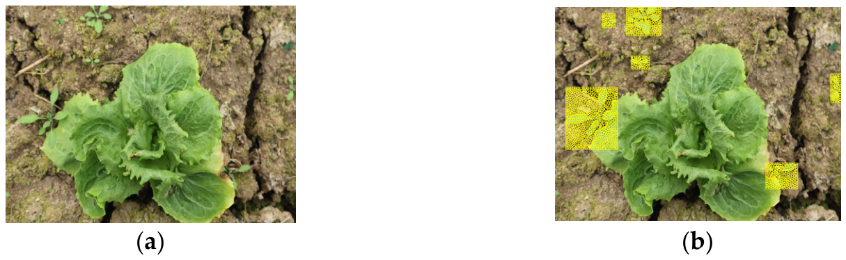
Although convolutional neural networks can perform target classification prediction for each pixel in an image, the convolution operation usually comprehensively considers the information of pixel neighborhoods. At target boundaries, pixels in the neighborhood may belong to different targets or the background at the same time, which may therefore introduce certain interference at target boundaries and lead to inaccurate segmentation of target boundaries [32]. In this paper, a superpixel segmentation method is used to perform fine over-segmentation on the original image. Adjacent pixels with similar feature information such as color and texture are divided into the same superpixel block. These superpixel blocks can closely fit the target contours or region boundaries closely, and different and continuous superpixel blocks constitute the complete original image. The SLIC (simple linear iterative clustering) algorithm proposed by Achanta et al. [33] is adopted for superpixel segmentation in this paper. The algorithm first initializes seed points of each pixel block uniformly in the original image and converts the image from the RGB color space to the lab color space. The positions of the seed points are dynamically adjusted according to the gradient changes of pixels in the lab color space. With the seed points as centers, an improved K-means clustering algorithm is used to perform local clustering of pixels, thereby generating superpixel blocks. The SLIC algorithm is implemented in Python3.8 to conduct superpixel segmentation on the ROI, and the results are shown in Figure 11.

To improve boundary consistency in overlapping or occluded weed regions, the network probability map is fused with the SLIC partition at the pixel level (Figure 12). SLIC supplies locally homogeneous regions rather than an independent semantic classifier; therefore, the category support of each superpixel is obtained from the network probabilities of the pixels contained in that region. The decision process consists of consensus retention and confidence-guided conflict resolution.

• Consensus retention: If the pixel-level network label agrees with the majority label of its SLIC superpixel, the label is retained directly. This operation leaves spatially coherent interior regions unchanged.
• Confidence-guided conflict resolution: When the pixel-level label disagrees with the majority label of its superpixel, the decision is made by comparing network confidence with superpixel homogeneity. A highly confident network prediction is retained, whereas an uncertain pixel is corrected by the locally consistent superpixel label.

For a reproducible implementation, let p_i ∈ [0, 1] denote the predicted weed probability of pixel i and let S_k be the SLIC superpixel containing that pixel. The pixel label is b_i = 1 when p_i ≥ 0.5 and b_i = 0 otherwise. The weed support ratio of S_k is q_k = |S_k|⁻¹ Σ_{j∈S_k} b_j, and its majority label is s_k = 1 when q_k ≥ 0.5 and s_k = 0 otherwise. Network confidence and superpixel homogeneity are defined as c_i = |2p_i − 1| and h_k = |2q_k − 1|, respectively. The final label is ŷ_i = b_i when b_i = s_k or c_i ≥ h_k; otherwise, ŷ_i = s_k. Thus, SLIC modifies only conflicting low-confidence pixels near locally coherent boundaries, while high-confidence network predictions are preserved. The fixed thresholds and SLIC settings used for reproducible re-training are summarized in Table 2.

3. Results and Analysis

This section reports the experimental environment and evaluation metrics, followed by analyses of data preprocessing, lightweight neck selection, module ablation, and comparison with representative segmentation models.

3.1. Experimental Environment and Parameter Setting

The hardware environment for training is as follows: the processor is an Intel Core i5-12490F running at 3.20 GHz, and the graphics card is a GeForce RTX 4060 Ti with 16 GB of video memory. The software environment is configured as: Windows 11 operating system, NVIDIA driver version 545.84, PyTorch-GPU 2.1.0 deep learning framework, CUDA version 12.1, and CUDNN deep neural network acceleration library version 8.8.1.

For reproducible re-training and independent verification, Table 2 specifies a standardized configuration to be applied consistently to the baseline, ablation variants, and comparison models. The same dataset split, preprocessing procedure, and hardware/software platform should be retained to prevent differences in training protocol from confounding model comparisons.

3.2. Evaluation Metrics

Four metrics are adopted to evaluate the segmentation performance of the model: pixel accuracy (PA), mean pixel accuracy (mPA), mean intersection over union (mIoU), and frequency weighted IoU (FWIoU). Their calculations are shown in Equations (12)–(15) [34].

$$PA={\displaystyle \frac{{\sum }_{i=0}^k{p_i}_i}{{\sum }_{i=0}^k{\sum }_{j=0}^k{p_i}_j}}$$

(12)

$$mPA={\displaystyle \frac{1}{k+1}}\sum _{i=0}^k{\displaystyle \frac{{p_i}_i}{{\sum }_{j=0}^k{p_i}_j}}$$

(13)

$$mIoU={\displaystyle \frac{1}{k+1}}\sum _{i=0}^k{\displaystyle \frac{{p_i}_i}{{\sum }_{j=0}^k{p_i}_j+{\sum }_{j=0}^k{p_j}_i-{p_i}_i}}$$

(14)

$$FWIoU={\displaystyle \frac{1}{{\sum }_{i=0}^k{\sum }_{j=0}^k{p_i}_j}}\sum _{i=0}^k{\displaystyle \frac{{\sum }_{j=0}^k{p_i}_j{p_i}_i}{{\sum }_{j=0}^k{p_i}_j+{\sum }_{j=0}^k{p_j}_i-{p_i}_i}}$$

(15)

To characterize false detections and missed detections, all test set pixels are accumulated in a pixel-level confusion matrix, the structure of which is shown in

Table 3. Pixel-level confusion matrix structure for binary weed segmentation.

Actual/Predicted	Weed	Non-Weed
Weed	TP	FN
Non-weed	FP	TN

For the binary task, true positive (TP) denotes weed pixels correctly classified as weed; false positive (FP) denotes non-weed pixels classified as weed; false negative (FN) denotes weed pixels classified as non-weed; and true negative (TN) denotes non-weed pixels correctly classified as non-weed.

Class-specific overlap is calculated directly from the same matrix: IoU_weed = TP/(TP + FP + FN) and IoU_non-weed = TN/(TN + FP + FN). Their arithmetic mean equals mIoU. This definition makes the treatment of the minority weed class explicit and prevents the dominant non-weed pixels from being represented only through overall PA.

On the basis of the above statistical quantities, two error metrics are adopted to quantitatively evaluate the false and missed detection magnitudes of the model. Type I error, also known as false positive error, corresponds to FP pixels and quantifies the false detection severity where the model misidentifies background or crop regions as weeds. This metric is numerically characterized by the false positive rate (FPR). A lower FPR signifies stronger anti-interference capability against complex field backgrounds and a reduced probability of false weed detection. Type II error, namely false negative error, corresponds to FN pixels and measures the missed detection degree when the model fails to capture genuine weed targets. It is quantified via the false negative rate (FNR). A lower FNR implies superior coverage performance for weed recognition and a lower chance of missing weed objects. The calculation formulas are presented in Equations (16) and (17).

$$FPR={\displaystyle \frac{FP}{FP+TN}}\times 100\%$$

(16)

$$FNR={\displaystyle \frac{FN}{TP+FN}}\times 100\%$$

(17)

3.3. Experimental Analysis of Data Preprocessing

To verify the effectiveness of data preprocessing and image enhancement in improving the robustness and generalization ability of the model, comparative experiments on the effects of super-resolution and data expansion were performed on the unimproved model. Expansion was carried out with multiples of 2, 3, and 4 to explore the optimal expansion multiple. The results are presented in

Table 4. Comparison of super-resolution and data expansion effects.

Super-Resolution	Expansion Multiple	Mean Pixel Accuracy mPA%
		Training Set	Test Set
×	None	80.1	73.8
√	None	81.2	74.8
×	2	81.5	80.9
√	2	82.4	81.8
×	3	83.4	83.6
√	3	84.3	84.7
×	4	83.7	82.8
√	4	84.5	83.7

Note: “√” indicates that the operation is performed, and “×” indicates that the operation is not performed.

.

According to Table 4, after performing super-resolution processing on the images, the mPA on the test set is improved by an average of 0.9 percentage points. Without image preprocessing and data expansion, the mPA on the test set is 6.3 percentage points lower than that on the training set, indicating that the model is limited by the number of training samples and suffers from overfitting during training, resulting in insufficient generalization ability. When the images are preprocessed and the data are expanded by a factor of 3, the mPA on the test set reaches the highest value of 84.7%, an improvement of 10.9 percentage points, which achieves the best effect in enhancing the generalization of the model. Therefore, super-resolution preprocessing and three-fold expansion are adopted for the dataset in this paper.

3.4. Performance Comparison of Different Neck Networks

To select the optimal lightweight neck architecture, four lightweight structures are compared with the standard convolution (SC) of the original network, namely depthwise separable convolution (DSC), Ghost Net, ShuffleNet, and GSConv. With the backbone network and detection head kept unchanged, the influence of each neck network on computational cost and segmentation accuracy is analyzed. The results are shown in

Table 5. Performance comparison of different neck networks.

Neck Network	mPA/%	mIoU/%	GFLOPs
SC	84.7	71.3	8.90
DSC	79.6	69.8	6.91
Shuffle Net	79.4	69.5	6.92
Ghost Net	82.5	70.3	7.21
GSConv	84.9	72.2	7.21

.

Compared with the original model, the [R7] GFLOPs (billions of floating point operations per forward pass) of the DSC- and ShuffleNet-based models are reduced by 1.99 × 10¹⁰ and 1.98 × 10¹⁰, respectively. However, DSC decreases mPA and mIoU by 5.1 and 1.5 percentage points, while ShuffleNet decreases them by 5.3 and 1.8 percentage points. GhostNet and GSConv both reduce GFLOPs by 1.69 × 10¹⁰; GSConv increases mPA and mIoU by 0.2 and 0.9 percentage points, whereas GhostNet decreases them by 2.2 and 1.0 percentage points. Thus, GSConv reduces theoretical computation while maintaining model accuracy. Accordingly, Table 5 supports a comparison of theoretical segmentation network computation only; GFLOPs are not interpreted as direct evidence of hardware-specific FPS, latency, or memory efficiency.

3.5. Ablation Experiment

To quantify both segmentation performance and computational cost after each modification, ablation experiments were conducted for every single module and their combinations; the results are listed in

Table 6. Ablation experiment results and computational cost after each modification.

Dual-ViT	GSConv	BiFPN	SLIC	PA/%	mPA/%	mIoU/%	FWIoU/%	GFLOPs
×	×	×	×	94	84.7	71.3	80.6	8.9
√	×	×	×	94	87.3	73.6	87.1	9.4
×	√	×	×	94	84.9	72.2	83.5	7.2
×	×	√	×	94	85.5	72.4	82.1	9.1
×	×	×	√	96	84.7	71.3	84.7	8.9
√	√	×	×	94	87.5	74.5	90	7.7
√	×	√	×	94	88.1	74.7	88.6	9.6
√	×	×	√	96	88.6	73.6	89.7	9.4
×	√	√	×	94	85.7	73.3	85	7.4
×	√	×	√	96	84.9	72.2	87.6	7.2
×	×	√	√	96	85.5	72.4	86.2	9.1
√	√	√	×	94	88.3	75.6	91.5	7.9
√	√	×	√	96	89.5	74.5	90.2	7.3
√	×	√	√	96	88.1	74.7	92.7	9.6
×	√	√	√	96	85.7	73.3	89.1	7.4
√	√	√	√	96	88.3	75.6	95.6	7.9

Note: “√” indicates that the operation is performed, and “×” indicates that the operation is not performed.

.

Table 6 shows that Dual-ViT changes mPA, mIoU, and FWIoU by +2.6, +2.3, and +6.5 percentage points at +0.5 GFLOPs; GSConv changes them by +0.2, +0.9, and +2.9 points while reducing GFLOPs by 1.7; and BiFPN changes them by +0.8, +1.1, and +1.5 points at +0.2 GFLOPs. SLIC alone leaves mPA and mIoU unchanged but increases PA and FWIoU by 2.0 and 4.1 points. With all four strategies, mPA, mIoU, and FWIoU increase by 3.6, 4.3, and 15.0 points, while GFLOPs decrease from 8.9 to 7.9.

The GFLOP values in Table 6 quantify only the segmentation network forward pass at the common input setting. Real-ESRGAN preprocessing and SLIC voting are external stages and are excluded from this architectural comparison. Consequently, the reported reduction represents relative network-level efficiency, whereas complete system throughput must be evaluated from the summed latency of Real-ESRGAN, DViT-YOLOv8-seg, and SLIC under one hardware platform. No real-time embedded operation claim is made from GFLOPs alone.

The ablation trends are consistent with the functional role of each component. Dual-ViT strengthens long-range context and local detail interaction, helping separate overlapping lettuce and weed regions; GSConv reduces redundant channel computation while retaining mixed features; BiFPN assigns adaptive weights to shallow and deep features, improving scale-dependent fusion; and SLIC enforces local color–texture consistency to correct isolated boundary pixels. Thus, the gains arise from complementary functions rather than from simple accumulation of modules.

3.6. Comparative Experiments of Different Models

To compare segmentation behavior, the proposed method was evaluated against YOLOv5-seg, DeepLabv3+, Fast-SCNN, and YOLOv10, with the segmentation results of different models shown in

Table 7. Comparison of different model performance.

Model	mPA/%	mIoU/%	GFLOPs
YOLOv5-seg	86.3	77.8	64.0
DeepLabv3+	88.6	84.3	176
Fast-SCNN	81.8	58.0	0.5
YOLOv10	90.1	74.2	59.1
Method in this paper	88.3	75.6	7.9

. In the uneven illumination and crop occlusion example in Figure 13, YOLOv5-seg produced fragmented boundaries and several soil false positives; Fast-SCNN missed portions of larger occluded weeds; and DeepLabv3+ generated relatively complete masks but required substantially greater theoretical network computation. YOLOv10 achieved a slightly higher mPA, whereas its GFLOPs were 7.47 times those of the proposed network. These visual differences are consistent with the intended roles of the proposed modules: global–local interaction helps preserve occluded weed continuity, weighted multi-scale fusion supports targets of different sizes, and superpixel voting removes isolated boundary errors. The comparison is therefore interpreted as an accuracy–theoretical–computation trade-off rather than proof of real-time deployment.

The proposed method exceeded YOLOv5-seg and Fast-SCNN in mPA by 2.0 and 6.5 percentage points, respectively, and was 1.8 percentage points below YOLOv10. Its mIoU of 75.6% was lower than that of DeepLabv3+ but higher than that of YOLOv10. The proposed network required 7.9 GFLOPs, 87.7%, 95.5%, and 86.6% lower than YOLOv5-seg, DeepLabv3+, and YOLOv10, respectively. Thus, the method provides a balanced compromise rather than superiority on every metric. The retained test set includes normal illumination, weak overcast light, backlighting, tree shade, uneven illumination, and crop–weed occlusion, so the reported results apply to the variability represented by this dataset. Figure 13 supplies qualitative evidence for a difficult combined condition; independent stratified tests across sites, seasons, cultivars, and phenological stages are still required before general field deployment.

3.7. Discussion and Scope of Applicability

The combined results show that the modules contribute complementary functions rather than uniformly improving every metric. The computational conclusions are restricted to network-level GFLOPs; end-to-end deployment assessment must include preprocessing and post-processing stages on the target platform. The robustness evidence is limited to the environmental variability contained in the current single-site dataset, and the binary formulation does not distinguish individual weed species. The evaluation framework therefore distinguishes weed and non-weed errors through the pixel-level confusion matrix, class-specific IoU, and Type I and Type II error definitions under one consistent protocol.

4. Conclusions

(1)

In this study, the dataset is augmented through super-resolution preprocessing and image enhancement, which effectively improves the generalization performance of the model. Ablation experiments show that the mean pixel accuracy of the original model on the test set has increased to 84.7%, with an improvement of 10.9 percentage points.

(2)

The complete method achieved 88.3% mPA, 75.6% mIoU, and 95.6% FWIoU at 7.9 network-level GFLOPs, showing that complementary feature extraction, fusion, and boundary correction can improve segmentation while maintaining moderate theoretical computation within the segmentation network.

(3)

Beyond the numerical gains, the scientific contribution is a task-oriented design showing how global–local representation, lightweight weighted multi-scale fusion, and superpixel boundary regularization can be coordinated for complex crop–weed scenes. The resulting pixel-level masks provide a perception basis for precision spraying, mechanical weeding, and offline field analysis systems. Future work will focus on cross-site and cross-season validation, species-aware segmentation, and optimized end-to-end implementation on edge platforms.

References

1. Calderara-Cea, F.; Torres-Torriti, M.; Cheein, F.A.; Delpiano, J. A two-stage deep learning strategy for weed identification in grassfields. Comput. Electron. Agric. 2024, 225, 109300. [Google Scholar] [CrossRef]
2. Hua, C.; Song, Y.; Jiang, Y.; Yu, J.; Chen, Y. RGB channel enhanced lawn weed recognition algorithm. J. Nanjing Agric. Univ. 2024, 47, 1019–1027. [Google Scholar]
3. Liang, C.; Wang, H.; Liu, X.; Tang, Q.; Zuo, C. Laser weeding weed detection method based on LSPKI-YOLO multi-scale feature enhancement. Trans. Chin. Soc. Agric. Eng. 2026, 42, 225–233. [Google Scholar]
4. Chen, X.; Xiong, Y.; Wang, X.; Cheng, N.; Liu, S.; Qi, L. Evaluation of weed density grade in paddy field seedling line zone based on tactile perception. Trans. Chin. Soc. Agric. Eng. 2023, 39, 116–125. [Google Scholar]
5. Chen, X.; Mao, Y.; Xiong, Y.; Qi, L.; Jiang, Y.; Ma, X. Intra-row weed density evaluation in rice field using tactile method. Comput. Electron. Agric. 2022, 193, 106699. [Google Scholar] [CrossRef]
6. Mao, Y.; Dang, P.; Zhang, E.; Tang, C.; Chen, Y.; Chen, X. Weed density evaluation using KCCA-CFBLS based on fusion of visual and tactile features in special paddy field environment. Comput. Electron. Agric. 2024, 217, 108619. [Google Scholar] [CrossRef]
7. Chen, X.; Dang, P.; Zhang, E.; Chen, Y.; Tang, C.; Qi, L. Accurate recognition of rice plants based on visual and tactile sensing. J. Sci. Food Agric. 2024, 104, 4268–4277. [Google Scholar] [CrossRef] [PubMed]
8. Gronewold, A.M.; Mulford, P.; Ray, E.; Ray, L.E. Tactile Sensing & Visually-Impaired Navigation in Densely Planted Row Crops, for Precision Fertilization by Small UGVs. Comput. Electron. Agric. 2025, 231, 110003. [Google Scholar] [CrossRef]
9. Miao, R.; Yang, H.; Wu, J.; Liu, H. Weed identification of overlapping spinach leaves based on image sub-block and reconstruction. Trans. Chin. Soc. Agric. Eng. 2020, 36, 178–184. [Google Scholar]
10. Zhang, S.; Huang, W.; Wang, Z. Combing modified Grabcut, K-means clustering and sparse representation classification for weed recognition in wheat field. Neurocomputing 2021, 452, 665–674. [Google Scholar] [CrossRef]
11. Osorio, K.; Pedraza, C.; Jamaica, D. A Deep Learning Approach for Weed Detection in Lettuce Crops Using Multispectral Images. AgriEngineering 2020, 2, 471–488. [Google Scholar] [CrossRef]
12. Hu, R.; Su, W.H.; Li, J.H.; Peng, Y. Real-time lettuce-weed localization and weed severity classification based on lightweight YOLO convolutional neural networks for intelligent intra-row weed control. Comput. Electron. Agric. 2024, 226, 109404. [Google Scholar] [CrossRef]
13. Sun, Y.; Chen, Y.; Jin, X.; Yu, J.; Chen, Y. AI Differentiation of Bok Choy Seedlings from Weed. Fujian J. Agric. Sci. 2021, 36, 1484–1490. [Google Scholar]
14. Jin, H.; Zhu, W.; Liu, T.; Yu, J.; Jin, X. Identification of vegetable weeds by using convolutional neural networks and color segmentation. J. Chin. Agric. Mech. 2024, 45, 215–220. [Google Scholar]
15. Wang, C.; Wu, X.; Zhang, Y.; Wang, W. Recognition and segmentation of maize seedlings in field based on dual attention semantic segmentation network. Trans. Chin. Soc. Agric. Eng. 2021, 37, 211–221. [Google Scholar]
16. Abdalla, A.; Cen, H.; Wan, L.; Rashid, R.; Weng, H.; Zhou, W.; He, Y. Fine-tuning convolutional neural network with transfer learning for semantic segmentation of ground-level oilseed rape images in a field with high weed pressure. Comput. Electron. Agric. 2019, 167, 105091. [Google Scholar] [CrossRef]
17. Cai, Y.; Xiao, J.; Yu, C.; Song, Z.; Li, J.; Yue, X. UANP-MT based semi-supervised image segmentation method for identifying weeds in cabbage field. Trans. Chin. Soc. Agric. Eng. 2023, 39, 183–191. [Google Scholar]
18. Syed, A.; Chen, B.; Abbasi, A.A.; Butt, S.A.; Fang, X. MSEA-Net: Multi-Scale and Edge-Aware Network for Weed Segmentation. AgriEngineering 2025, 7, 103. [Google Scholar] [CrossRef]
19. Wang, X.; Xie, L.; Dong, C.; Shan, Y. Real-ESRGAN: Training Real-World Blind Super-Resolution with Pure Synthetic Data. In Proceedings of the IEEE/CVF International Conference on Computer Vision Workshops, Montreal, BC, Canada, 11–17 October 2021; IEEE: Piscataway, NJ, USA, 2021; pp. 1905–1914. [Google Scholar]
20. Yang, T.; Wei, W.; Fu, C.; Yang, T. Single-image super-resolution reconstruction based on improved Real-ESRGAN. Mod. Electron. Technol. 2025, 48, 31–38. [Google Scholar]
21. Wang, X.; Yu, K.; Wu, S.; Gu, J.; Liu, Y.; Dong, C.; Loy, C.C.; Qiao, Y.; Tang, X. ESRGAN: Enhanced Super-Resolution Generative Adversarial Networks. In Proceedings of the European Conference on Computer Vision Workshops, Munich, Germany, 8–14 September 2018. [Google Scholar]
22. Chen, S.; Xu, L.; Zhou, B.; Chen, J. Semantic Relocation Parallel Network for Semantic Segmentation. J. Comput. Aided Des. Comput. Graph. 2022, 34, 373–381. [Google Scholar] [CrossRef]
23. Vaswani, A.; Shazeer, N.; Parmar, N.; Uszkoreit, J.; Jones, L.; Gomez, A.N.; Kaiser, L.; Polosukhin, I. Attention is All you Need. In Proceedings of the Neural Information Processing Systems, Long Beach, CA, USA, 12 June 2017. [Google Scholar]
24. Liu, L.; Li, G.; Du, Y.; Li, X.; Wu, X.; Qiao, Z.; Wang, T. CS-Net: Conv-Simpleformer network for agricultural image segmentation. Pattern Recognit. 2024, 147, 110140. [Google Scholar] [CrossRef]
25. Yao, T.; Li, Y.; Pan, Y.; Wang, Y.; Zhang, X.P.; Mei, T. Dual Vision Transformer. IEEE Trans. Pattern Anal. Mach. Intell. 2023, 45, 10870–10882. [Google Scholar] [CrossRef] [PubMed]
26. Li, J.; Wen, Y.; He, L. SCConv: Spatial and Channel Reconstruction Convolution for Feature Redundancy. In Proceedings of the IEEE/CVF Conference on Computer Vision and Pattern Recognition, Vancouver, BC, Canada, 17–24 June 2023; IEEE: Piscataway, NJ, USA, 2023; pp. 6153–6162. [Google Scholar]
27. Li, H.; Li, J.; Wei, H.; Liu, Z.; Zhan, Z.; Ren, Q. Slim-neck by GSConv: A lightweight-design for real-time detector architectures. J. Real-Time Image Process. 2024, 21, 62. [Google Scholar] [CrossRef]
28. Yang, Q.; Ye, Y.; Gu, L.; Wu, Y. MSFCA-Net: A Multi-Scale Feature Convolutional Attention Network for Segmenting Crops and Weeds in the Field. Agriculture 2023, 13, 1176. [Google Scholar] [CrossRef]
29. Wang, Y.; Chen, Q.; Wu, J. Research on Image Semantic Segmentation for Complex Environments. Comput. Sci. 2019, 46, 36–46. [Google Scholar]
30. Guo, Q.; Liu, L.; Zhang, C.; Xu, W.; Jing, W. Muti-scale Feature Fusion Network Based on Feature Pyramid Model. Chin. J. Eng. Math. 2020, 37, 521–530. [Google Scholar]
31. Tan, M.; Pang, R.; Le, Q.V. EfficientDet: Scalable and Efficient Object Detection. In Proceedings of the IEEE/CVF Conference on Computer Vision and Pattern Recognition, Seattle, WA, USA, 13–19 June 2020; IEEE: Piscataway, NJ, USA, 2021; pp. 10778–10787. [Google Scholar]
32. Wang, L.; Zhang, S.; Zhong, X.; Li, M.; Ma, Z. GDBNet: Boundary improving three-branch semantic segmentation network for remote sensing images. J. Electron. Imaging 2024, 33, 063019. [Google Scholar] [CrossRef]
33. Achanta, R.; Shaji, A.; Smith, K.; Lucchi, A.; Fua, P.; Süsstrunk, S. SLIC Superpixels Compared to State-of-the-Art Superpixel Methods. IEEE Trans. Pattern Anal. Mach. Intell. 2012, 34, 2274–2282. [Google Scholar] [CrossRef] [PubMed]
34. Yu, Y.; Wang, C.; Fu, Q.; Kou, R.; Wu, W.; Liu, T. Survey of Evaluation Metrics and Methods for Semantic Segmentation. Comput. Eng. Appl. 2023, 59, 57–69. [Google Scholar]
Figure 1. The overall workflow of the segmentation method.
Agriculture 16 01675 g001
Figure 2. Super-resolution network architecture and super-resolution effect diagram. (a) Structure of Real-ESRGAN generator; (b) original image of local weed; (c) super-resolution effect image of local weed.
Agriculture 16 01675 g002
Figure 3. Image enhancement diagram. (a) Original image; (b) contrast adjustment; (c) salt-and-pepper noise; (d) bounding box-level rotation; (e) Cutout augmentation; (f) Mixup augmentation.
Agriculture 16 01675 g003
Figure 4. C2f-DViT module.
Agriculture 16 01675 g004
Figure 5. Dual-vision Transformer backbone structure diagram. (a) Dual block; (b) merge block.
Agriculture 16 01675 g005
Figure 6. Structure of GSConv.
Agriculture 16 01675 g006
Figure 7. Structure of GS bottleneck.
Agriculture 16 01675 g007
Figure 8. Structure of VoVGSCSP.
Agriculture 16 01675 g008
Figure 9. Different feature fusion layer structure. (a) FPN; (b) PAN; (c) BiFPN; (d) improved BiFPN.
Agriculture 16 01675 g009
Figure 10. Improved YOLOv8-seg network model structure.
Agriculture 16 01675 g010
Figure 11. Superpixel segmentation. (a) Original image; (b) result of superpixel segmentation.
Agriculture 16 01675 g011
Figure 12. Superpixel segmentation and weed recognition workflow.
Agriculture 16 01675 g012
Figure 13. Segmentation results of different models. (a) Original image; (b) YOLOv5-seg; (c) DeepLabv3+; (d) Fast-SCNN; (e) YOLOv10; (f) method in this paper.
Agriculture 16 01675 g013