CFD-Based Simulation and Optimization of Summer Environmental Conditions in Laying Hen Houses

Abstract

To address uneven temperature and relative humidity distributions, localized heat accumulation, and insufficient air velocity in an enclosed stacked-cage laying hen house, a three-dimensional computational fluid dynamics (CFD) model of the laying hen house was developed using field-measured structural and environmental data, and a porous-media model was established for the cage zone. Model validation showed that the normalized mean square error (NMSE) values for temperature, relative humidity, and air velocity were all below 0.25, confirming the reliability of the CFD model. Through visualization analysis of the contour maps, the problems of uneven airflow distribution in the original ventilation system and significant heat accumulation at the fan end were identified. On this basis, numerical simulations were conducted for six air-inlet configurations by varying two key parameters: air-inlet spacing and air-inlet number. The simulation results showed that, compared with the original model, the configuration with an air-inlet spacing of 1.14 m and a total of 32 air inlets on the two gable walls improved the uniformity of temperature, air velocity, and relative humidity by 18.00%, 10.54%, and 18.38%, respectively, while reducing the mean effective temperature index (ETI) in the cage zone by 0.5 °C. This configuration effectively alleviated localized heat accumulation and improved air-velocity uniformity. These findings provide a theoretical basis and technical support for the structural optimization and environmental regulation of enclosed stacked-cage laying hen houses.

1. Introduction

Modern egg production has been shifted toward scale and mechanization, making environmental control in layer houses increasingly critical [1]. It has been demonstrated that high-temperature environments in summer can lead to a decrease in the egg production rate of laying hens increase in the feed-egg ratio [2], resulting in significant economic losses. The thermal comfort in layer houses is largely determined by environmental temperature, relative humidity, and air velocity, which directly influence the physiological health [3,4,5] and production performance [6,7,8,9,10,11] of the flock. Ventilation plays a key role in achieving a desirable thermal environment in layer houses. Poor ventilation may result in localized uncomfortable conditions for birds, but also elevated concentrations of pollutants such as carbon dioxide (CO₂), ammonia (NH₃), and hydrogen sulfide (H₂S), which may also adversely affect the production performance of the birds.

Various approaches have been used to optimize the design of ventilation systems in animal buildings, and one of these approaches is Computational Fluid Dynamics (CFD). With the rapid advancement of computer processing power and the gradual refinement of fundamental CFD theory, this powerful engineering tool has been widely applied in recent years in the field of agricultural and livestock engineering to address issues in environmental control within livestock and poultry housing [12,13,14,15]. CFD enables relatively accurate simulation of indoor airflow velocity and temperature field distributions [16,17,18], providing a foundation for optimization of ventilation design, and thus improvement of the thermal environment for animals. For example, CHOI et al. [19] developed and validated a CFD model for predicting dynamic temperature changes caused by ventilation operations (such as fan activation and deactivation, and inlet adjustments) in commercial broiler houses, and they found that adjusting the inlet layout could alleviate localized high temperatures. KEYVAN et al. [20] used CFD simulations to optimize the tunnel-ventilated layer house environment. They proposed a new model with 15 fans and 3 evaporative cooling pads arranged on the east and west walls, respectively. This model significantly improved indoor airflow uniformity (wind speed of 2.5 m/s at bird height), temperature distribution (maximum 35 °C), humidity (60–75%), and concentrations of CO₂ and NH₃ pollutants. Recent studies have already examined summer ventilation in commercial laying hen houses from several perspectives. Chen et al. [21] further developed an all-year sidewall-inlet ventilation system incorporating buffer spaces and a constant inlet arrangement to stabilize the hen-level thermal environment in a commercial multi-tier laying hen house. Zhang et al. [22] established ventilation-resistance and fan-performance relationships for estimating tunnel-fan operating conditions in a laying hen house. These studies demonstrate that summer ventilation in commercial laying hen houses has been actively investigated. Although CFD-based studies have substantially advanced the environmental design of poultry houses, most previous optimization efforts have focused either on individual structural components or on the overall rearrangement of fans, cooling pads, and airflow-guiding devices. Comparatively little attention has been given to the coupled mechanism through which air-inlet configuration, aerodynamic resistance within the cage zone, and longitudinal airflow attenuation jointly govern the delivery of cooled air to different cage tiers. Consequently, improvements in whole-house mean environmental conditions do not necessarily result in a corresponding reduction in thermal exposure within the hen-occupied zone, particularly in long, high-density, multi-tier laying hen houses. This unresolved scale mismatch between system-level ventilation performance and cage-tier microclimate regulation restricts the practical application of CFD-based optimization strategies to existing commercial facilities. A cage-zone-oriented optimization framework is therefore required to link inlet-induced airflow redistribution with tier-resolved environmental uniformity and integrated thermal-stress assessment.

To address these limitations, this study developed a three-dimensional computational fluid dynamics (CFD) model of a commercial multi-tier stacked-cage laying hen house located in the subtropical region of Huangshan, Anhui Province, China (29°42′41″ N, 118°18′45″ E), and validated the model against field measurements. Because the cage structures and densely stocked hens substantially influence momentum, heat, and moisture transport, the hen-occupied cage zone was represented as a porous medium. The validated CFD model was then used to evaluate six combinations of air-inlet number and horizontal spacing and to quantify their effects on air temperature, relative humidity, air velocity, environmental uniformity, and the effective temperature index at both cage-zone and cage-tier scales. The objectives were to clarify how inlet-induced airflow redistribution affects cooling-air penetration and thermal exposure within the hen-occupied region and to identify a practical air-inlet layout for improving ventilation effectiveness and thermal uniformity in existing commercial laying hen houses.

2. Materials and Methods

2.1. Experimental Site and Measurements

2.1.1. Experimental Laying Hen House and Flock

The experimental laying hen house was 90 m long, 15 m wide, and 7.5 m high and was roofed with reddish-brown color-coated steel sheets. The house used a five-tier, five-row stacked-cage system. Five rows of production equipment were installed, with hens housed on both sides of each row and in five tiers on each side. Each row comprised 40 cage groups, and each group consisted of three cages (eight hens per cage; cage dimensions: 70 cm × 60 cm × 50 cm). The floor area available per hen was 0.0525 m². The house accommodated approximately 48,000 29-week-old Hy-Line Brown laying hens. The building was oriented north–south and operated under longitudinal ventilation. The north wall was the cooling-pad end and served as the air-inlet wall, whereas the south wall was the exhaust-fan end and served as the air-outlet wall. The east and west sidewalls were equipped with cooling pads of equal area and equal numbers of ventilation windows. At the cooling-pad end of each sidewall, two rows of air inlets were installed, with an equal number of inlets in each row. Each air inlet was fitted with an air deflector. The cages, exhaust fans, and other production equipment were custom-manufactured by Guangzhou Guangxing Animal Husbandry Equipment Group Co., Ltd., Guangzhou, China. The laying hen house is shown in Figure 1, and the main parameters measured on site are listed in

Table 1. Main parameters of the laying hen house.

Parameter	Parameter Value	Parameter	Parameter Value
Laying hen house Length/m	90	Number of air deflectors	29
Laying hen house width/m	15	Air deflector length/m	2
Laying hen house wall height/m	5.5	Air deflector width/m	1
Roof pitch height/m	2.0	Number of ventilation windows	60
Fan diameter/m	1.32	Ventilation window length/m	0.7
Number of production equipment units	5	Ventilation window width/m	0.25
Corridor width/m	1.1	Number of fans/units	18
Cooling pad area/m2	189.42	Ventilation method	Negative pressure ventilation

.

2.1.2. Measurement Instruments

The environmental variables measured in the laying hen house included air temperature, relative humidity, and air velocity. Air temperature, relative humidity, illuminance, and CO₂ concentration were measured using an integrated four-in-one sensor (ST-BYX; Guangzhou Saitong Technology Co., Ltd., Guangzhou, China). Air velocity was measured using an HD403TS2 anemometer (Delta OHM, Padova, Italy). All sensors were factory-calibrated before use and communicated with an MCGS human–machine interface through the RS-485 protocol. The sensor specifications are listed in

Table 2. Specifications of sensors for environment monitoring.

Environmental Parameters	Range	Resolution	Accuracy
Temperature/°C	−40–80	0.1	±0.5
Relative Humidity/RH	0–100%	0.1%	±3%
Illuminance/lux	0–100	1.0	±1%
CO2/(ppm)	0–5000	1.0	±100
Air velocity/(m·s−1)	0–5	0.0001	±(0.2 + 3%f.s)

.

2.1.3. Field Measurements

Field measurements were conducted from 3 July to 31 August 2024. Monitoring locations were established at the front, middle, and rear sections of the cage rows. At each longitudinal location, two vertically aligned monitoring points were positioned at the center of the aisle, at heights of 0.55 and 1.15 m above the floor, corresponding to the mid-heights of the first and second cage tiers, respectively. A total of 18 monitoring points were arranged at each height, resulting in 36 monitoring points throughout the laying hen house. Air temperature, relative humidity, and air velocity were recorded at each monitoring location during three daily periods: 06:00–08:00, 12:00–14:00, and 18:00–20:00. Temperature and relative humidity were also measured at the cooling-pad inlets at the front end, the fan outlets at the rear end, and the interior wall surfaces of the laying hen house. At 08:30 each day, eggs were manually collected, and the egg mass from the three cage groups corresponding to each monitoring location was measured using a Songjing electronic scale (Wuyi Zhuheng Electronic Co., Ltd., Wuyi, China). On 31 August 2024, three hens were randomly selected from the three cage groups corresponding to each monitoring location and weighed using the same electronic scale. The monitoring locations are shown in Figure 2.

2.2. CFD Modeling

2.2.1. Geometric Model and Meshing

A three-dimensional model of the laying hen house was constructed using SpaceClaim 2023 R1. A 1:1 geometric model was established according to the actual dimensions and geometric relationships of the laying hen house. The exhaust fans on the south wall were represented as circular openings with a diameter of 1.32 m. The cooling-pad air inlets on the north wall, together with the air inlets located at the cooling-pad ends of the east and west sidewalls, were represented as rectangular openings measuring 2 m × 1 m. The opening angle of the air-inlet deflectors was fixed at 30°, and the horizontal and vertical spacings between adjacent air inlets were 1.14 m and 1.0 m, respectively. The rectangular ventilation windows on the east and west sidewalls remained closed during summer daytime operation and were therefore treated as solid walls in the CFD model. Internal equipment, including the automatic feeding system, automatic drinking system, and feed troughs, was omitted because of its complex geometry and relatively limited influence on the predicted airflow and thermal environment. The laying hens and cage structures were simplified as rectangular blocks measuring 85.1 m × 1.27 m × 0.5 m. The resulting simplified geometric model of the laying hen house is shown in Figure 3.

2.2.2. Mesh Generation

The constructed laying hen house model was imported into the ANSYS 2023R1 software. Mesh generation was performed using Poly-Hexcore technology within the Fluent Mesh. Setting the minimum cell length for the model body to 50 mm and a maximum volume element length of 200 mm yielded 4, 297,145 elements. The minimum, maximum, and average orthogonal quality factors were 0.34, 1.0, and 0.92, respectively. This suggests that the mesh possesses a high quality, making it suitable for subsequent computational analyses using the Fluent solver [23]. The partitioning of the mesh for the laying hen house is illustrated in Figure 4.

2.2.3. Mesh Independence Test

A mesh-independence test was conducted to determine an appropriate mesh resolution. Eight meshes containing 945,017 to 7,183,987 cells were generated using different cell sizes (Figure 5). Steady-state simulations were performed for the morning, midday, and evening conditions. Two horizontal monitoring planes were established at heights of 0.55 and 1.15 m, corresponding to the sensor locations used in the field measurements. Mesh independence was assessed using the mean air velocity on the 1.15 m plane. The mean air velocity gradually stabilized as the number of cells increased, and only minor changes were observed when the mesh contained approximately 4 million cells. Further mesh refinement had little effect on the predicted air velocity. Therefore, the mesh containing 4,297,145 cells was selected for all subsequent simulations. For this mesh, the minimum and maximum cell sizes were 50 and 200 mm, respectively, and the minimum, maximum, and mean orthogonal quality values were 0.34, 1.00, and 0.92, respectively. These values indicated that the mesh quality met the requirements for the subsequent numerical calculations.

2.3. Boundary Condition Settings in ANSYS Fluent

2.3.1. Initial and Boundary Condition Settings

During field data collection, the indoor and outdoor environmental conditions remained stable, the cooling pads and exhaust fans operated normally, and the inlet and outlet configurations remained unchanged. Therefore, steady-state simulations were performed. Gravitational acceleration was set to −9.81 m/s² in the Z direction. The initial temperature of the indoor computational domain was set to 30.36 °C, corresponding to the mean temperature measured at all field monitoring locations. The energy equation and species transport model were enabled to simulate heat and moisture transfer within the laying hen house.

The ideal-gas formulation was adopted because it adequately represents the thermophysical properties of air while maintaining computational efficiency, making it well suited for steady-state simulations of airflow and temperature distributions in laying hen houses [24]. Accordingly, the gas phase was defined as a mixture of dry air and water vapor and modeled using the incompressible ideal-gas density law, with density variations assumed to arise solely from changes in temperature [25].

2.3.2. Turbulence Model

Research has demonstrated that under conditions of limited experimental data, the Realizable k-ε turbulence model is capable of maintaining relatively high accuracy [26,27,28], and it outperforms the Standard k-ε and RNG k-ε models in simulating strongly curved streamlines and vortices [29,30]. Therefore, the Realizable k-ε model was adopted in this study.

2.3.3. Boundary Conditions

The experimental laying hen house was operated under a longitudinal negative-pressure ventilation system. Outdoor air entered the house through the rectangular inlets at the cooling-pad end, flowed longitudinally through the building, and was ultimately exhausted to the outdoor environment by the fans at the opposite end. Accordingly, the cooling-pad inlets were specified as velocity-inlet boundaries in the numerical model. The inlet conditions were determined from the mean values of the measured environmental data, comprising an air temperature of 28.24 °C, an air velocity of 3.48 m/s, and a relative humidity of 87%. Based on the psychrometric chart, the corresponding water-vapor mass fraction was calculated as 0.02154. Because the fan end constituted the only airflow outlet from the house, it was specified as a pressure-outlet boundary with a static gauge pressure of 0 Pa. All surfaces of the building envelope were prescribed as isothermal no-slip walls. The boundary conditions are summarized in

Table 3. Boundary Condition Settings.

Variable	Location	Boundary Type	Boundary Parameter	Parameter Value
Wall Surface	East Wall	Non-slip Wall Surface	Temperature/°C	29.76
	West Wall			30.01
	South Wall			28.96
	North Wall			30.92
	Floor			29.29
	East Roof			30.36
	West Roof			30.88
Air Inlet	Evaporative Cooling Pad End	Velocity Inlet	Temperature/°C	28.24
			Wind Speed/(m·s−1)	3.48
			Water Vapor Mass Fraction	0.02154
Outlet	Fan End	Pressure Outlet	Static Pressure/Pa	0

. All values reported in the table were obtained by averaging the field measurements collected at the corresponding locations during the midday period from 12:00 to 14:00.

2.3.4. Boundary Conditions for the Cage Zone

When the cage assemblies are represented as impermeable solid blocks in steady-state CFD simulations, airflow cannot penetrate the cage zone, and the predicted temperature, relative humidity, and air-velocity fields are limited to the surrounding air domain. In the actual laying hen house, however, air flows through both the cages and the spaces occupied by the hens. Therefore, the cage assemblies and laying hens were represented as a porous-medium region in the present model. This treatment enabled the airflow and the associated temperature and relative humidity distributions within the cage zone to be resolved, thereby providing a more realistic representation of the microenvironment experienced by the hens.

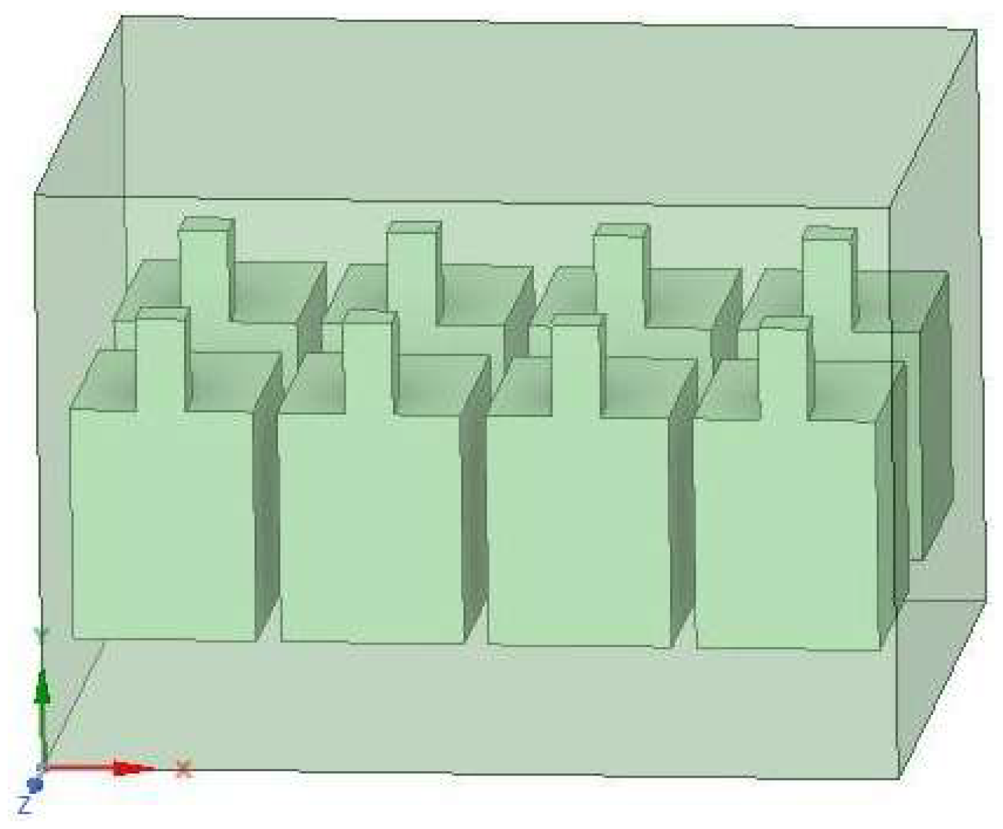
An appropriate simplified geometry of an individual hen was first selected to determine the solid volume occupied within the porous-medium region. Cheng et al. [31] evaluated three geometric representations of a hen, namely a simplified hen model, a body-shaped model, and an ellipsoidal model, and selected the simplified hen model based on comparative CFD simulations. Zhang [32] subsequently compared the simplified hen model with a cuboid hen model and reported that the cuboid representation produced better mesh quality and required less computational effort. Accordingly, the cuboid hen model was adopted in this study. An actual cage measuring 0.70 m × 0.50 m × 0.60 m and housing eight hens was used to define the porous-medium volume. Each hen was represented by two cuboids: a neck measuring 0.04 m × 0.04 m × 0.08 m and a body measuring 0.15 m × 0.20 m × 0.25 m. The legs were neglected during geometric simplification. The geometric porosity of the representative cage-and-hen region was calculated from the ratio of the void volume to the total cage volume. The total volume of the representative cage was 0.210 m³, whereas the simplified solid volume occupied by the eight hens was 0.0610 m³. 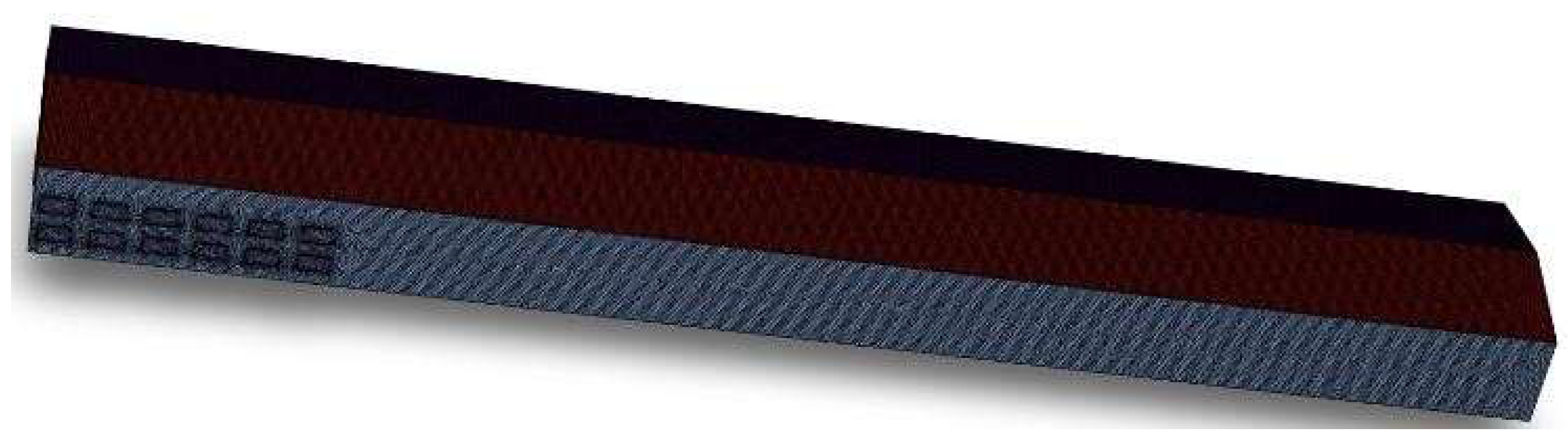Accordingly, the geometric porosity was calculated as ε = 1 − V_s/V_p = 0.709 nd was set to 0.71 in the porous-medium model. The volume of the cage wires was not included in this geometric calculation; their overall aerodynamic effect, together with that of the hens, was represented by the direction-dependent viscous and inertial resistance coefficients obtained from the velocity–pressure-drop fitting procedure described below. The resulting geometric representation is shown in Figure 6.

The pressure drop across a porous medium is governed by the superficial velocity through the medium. Therefore, determination of the viscous and inertial resistance coefficients in each principal direction requires establishing the relationship between the pressure drop and the corresponding superficial velocity. This relationship is described by Equation (1):

$$∆\mathrm{P}/∆\mathrm{n}={\mathrm{D}}_1\mathrm{u}\mathrm{v}+{\displaystyle \frac{1}{2}}{\mathrm{C}}_2\mathsf{\rho }{\mathrm{v}}^2$$

(1)

where ∆P/∆n represents the pressure drop per meter (Pa/m); D₁ is the viscous resistance coefficient (m⁻²); v is the airflow velocity (m/s); C₂ is the inertial resistance coefficient (m⁻¹); μ is the dynamic viscosity of air (N·s/m²) (1.7894 × 10⁻⁵ N·s/m²); and ρ is the air density (kg/m³) 1.225 kg/m³ [23]).

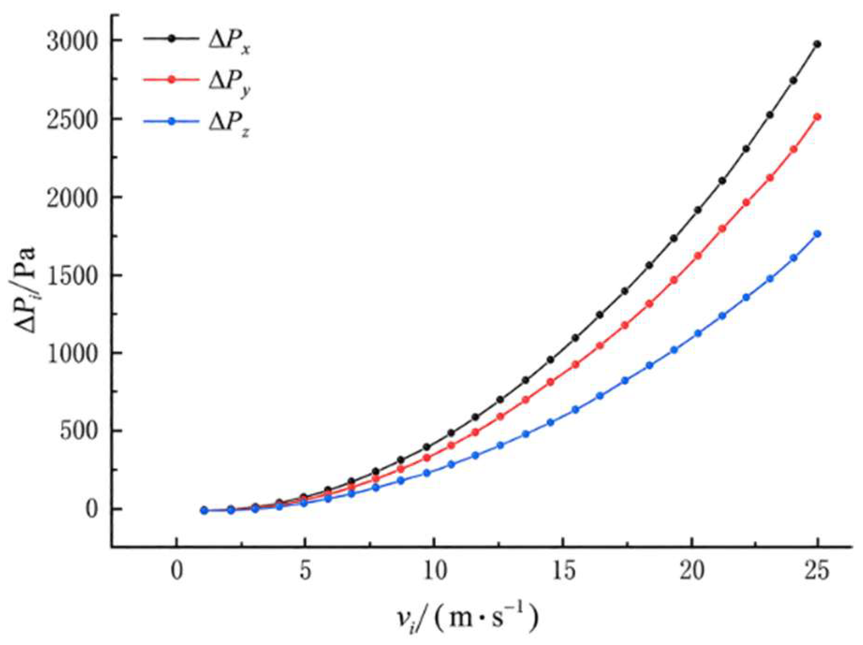
For the X-, Y-, and Z-directions, a series of incrementally varied inlet velocities was prescribed separately, and the corresponding pressure drops between the upstream and downstream faces of the porous-medium model were recorded. The data were then fitted using Equation (1) to establish the velocity–pressure-drop relationship in each direction, as shown in Figure 7.

The relationship between velocity and pressure drop in each direction was derived through curve fitting and is given by Equation (2) as follows:

$$\{\begin{array}{c}{∆P}_x/∆n=4.74441v_x^2+0.05528v_x\\ {∆P}_y/∆n=3.97618v_y^2+1.05886v_y\\ {∆P}_z/∆n=2.76358v_z^2+0.66779v_z\end{array}$$

(2)

By combining Equation (2) with Equation (1), the viscous and inertial resistance coefficients in each direction were determined. In the calculations, μ and ρ were set to 1.7894 × 10⁻⁵ N·s/m² and 1.225 kg/m³, respectively. The resulting coefficients for the porous-medium model in the X, Y, and Z directions are listed in

Table 4. Coefficient of resistance of porous media.

Porous-Medium Direction	X	Y	Z
Viscous resistance coefficient, D1 (m−2)	4.413 × 103	1.183 × 105	6.22 × 104
Inertial resistance coefficient, C2 (m−1)	11.0657	12.9834	7.5199

.

The porous-medium zone was also defined as a volumetric heat source. Because the heat production of an individual hen varies with ambient temperature, total heat production was calculated as the sum of sensible and latent heat production using the equations recommended by the International Commission of Agricultural and Biosystems Engineering (CIGR), as given in Equations (3)–(5) [30]. The volumetric heat generation rate and volumetric moisture production rate of the porous-medium zone were subsequently calculated using Equations (6) and (7), respectively.

$${\Phi }_{tot}={\displaystyle \frac{\left[1000+20\times \left(20-T\right)\right]}{1000}}\times \left(6.28m^{0.75}+25Y_2\right)$$

(3)

$${\Phi }_s={\displaystyle \frac{\left[670+13.4\times \left(20-T\right)-9.80\times {10}^{-8}\times T^6\right]}{1000}}\times \left(6.28m^{0.75}+25Y_2\right)$$

(4)

$${\Phi }_l=\Phi -{\Phi }_s$$

(5)

$$Q_s={\Phi }_s\times {\displaystyle \frac{n}{V}}$$

(6)

$$M_l={\displaystyle \frac{{\Phi }_l}{r}}\times {\displaystyle \frac{n}{V}}$$

(7)

where Φ_tot is the total heat production by a laying hen, W; Φ_s is the sensible heat produced by a laying hen, W; Φ_l is the latent heat produced by a laying hen, W; T is the air temperature, °C; m is the average weight of a laying hen, kg; Y₂ is the egg production, kg/day; Q_S is the sensible heat production rate per unit volume, W/m³; M_l is the moisture production rate per unit volume, kg/m³·s; V is the cage volume, m³; r is the latent heat of vaporization of water, kJ/kg; n is the number of laying hens in a cage.

The specification of source terms in the porous-medium zone is a critical component of the numerical simulation of the thermal and moisture environment within the laying hen house. In this study, all source-term parameters were determined from field measurements. The measured inputs included eight hens per cage, a mean indoor air temperature of 30.36 °C, a mean body mass of 1.992 kg per hen, a mean daily egg mass of 0.5845 kg d⁻¹, and a total of 1920 hens represented by each porous-medium computational domain. Based on these measured parameters, the heat and moisture production of the hens was quantified using the corresponding empirical equations. The calculated volumetric heat generation rate and volumetric moisture production rate of the porous-medium zone were 193.61 W m⁻³ and 5.9332 × 10⁻⁵ kg m⁻³ s⁻¹, respectively.

2.3.5. Validation of the Laying Hen House Model

The CFD model was validated to assess the reliability and accuracy of the simulation results. Model performance was quantified using the mean relative error (MRE) and normalized mean square error (NMSE). Environmental data measured at monitoring locations corresponding to the first and second cage tiers were compared with the simulated values. An NMSE below 0.25 was considered to indicate acceptable predictive accuracy [33,34]. The calculation procedures are given in Equations (8)–(10).

$$MRE={\displaystyle \frac{\sum _{i=1}^n\frac{\left|C_{si}-C_{mi}\right|}{C_{mi}}}{n}}$$

(8)

$$NMSE={\displaystyle \frac{{\left(\overline{C_s-C_m}\right)}^2}{C_{sv}{C}_{mv}}}$$

(9)

$${\left(\overline{{\mathrm{C}}_{\mathrm{s}}-{\mathrm{C}}_{\mathrm{m}}}\right)}^2={\displaystyle \frac{\sum _{\mathrm{i}=1}^{\mathrm{n}}{\left({\mathrm{C}}_{\mathrm{si}}-{\mathrm{C}}_{\mathrm{mi}}\right)}^2}{\mathrm{n}}}$$

(10)

MRE denotes the mean relative error between the simulated and measured values; C_s represents the simulated value; C_m denotes the measured value; C_sv signifies the mean simulated value; C_mv indicates the mean measured value; and n denotes the number of monitoring points.

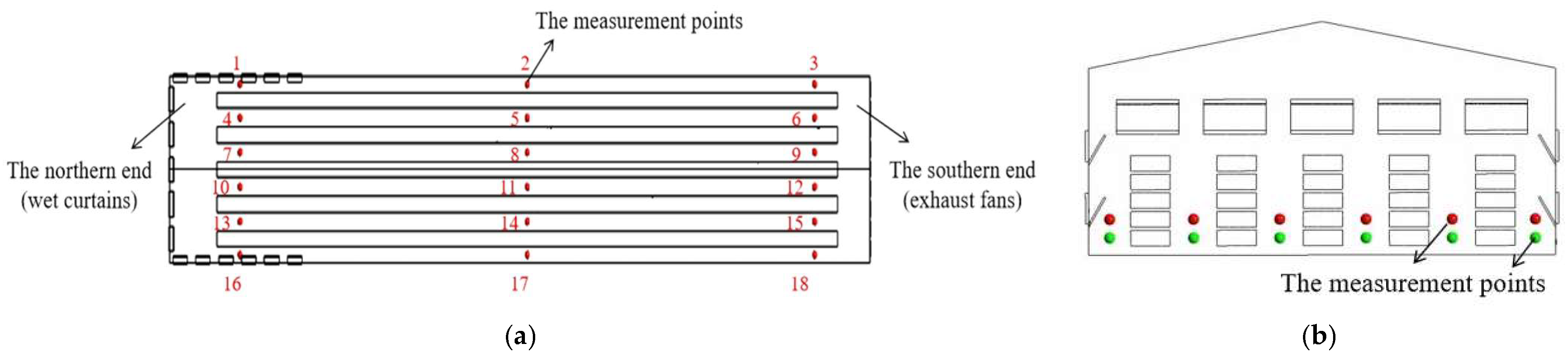
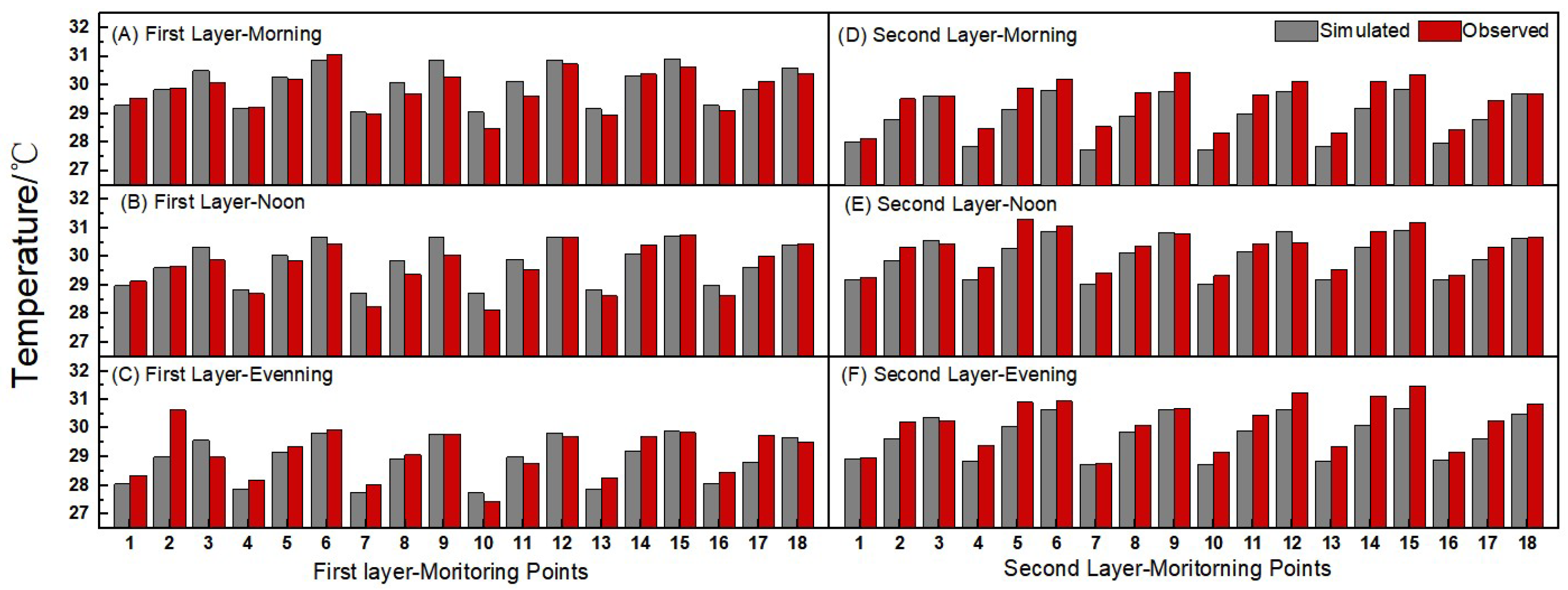
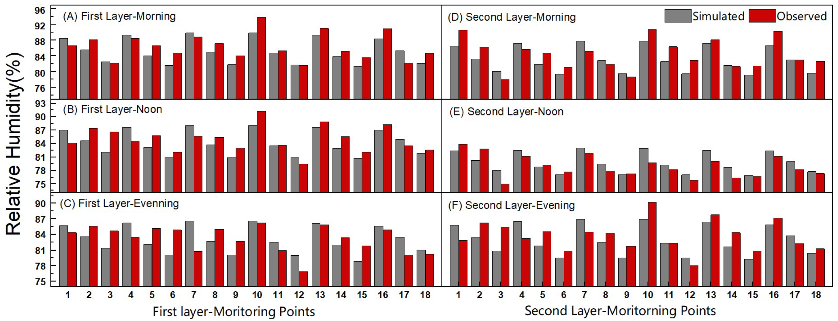
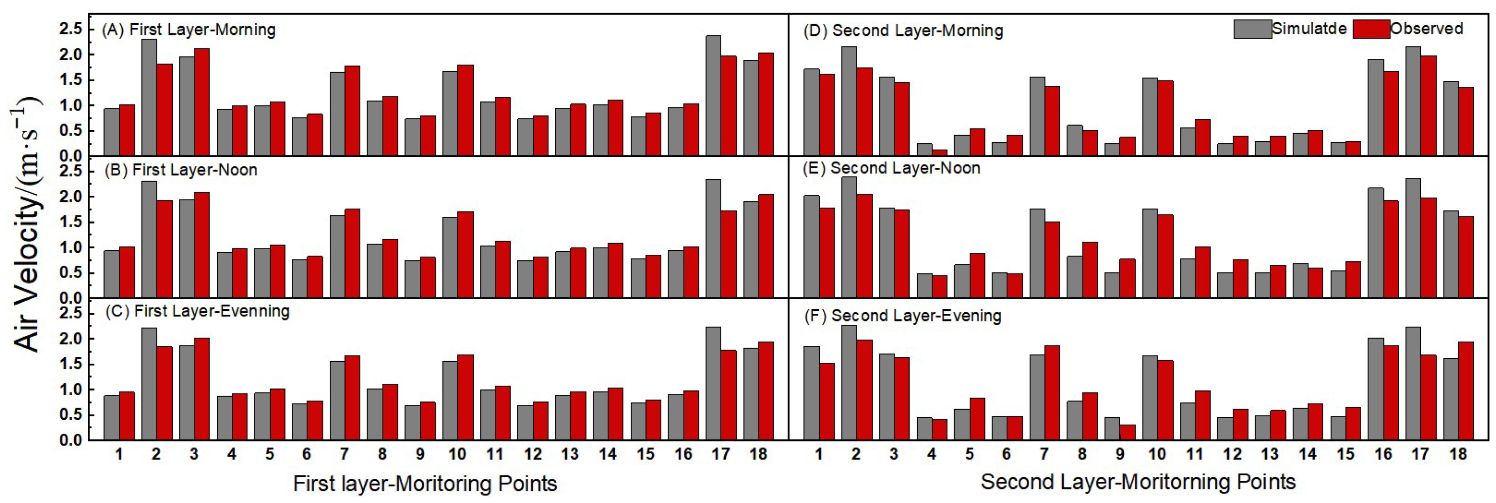
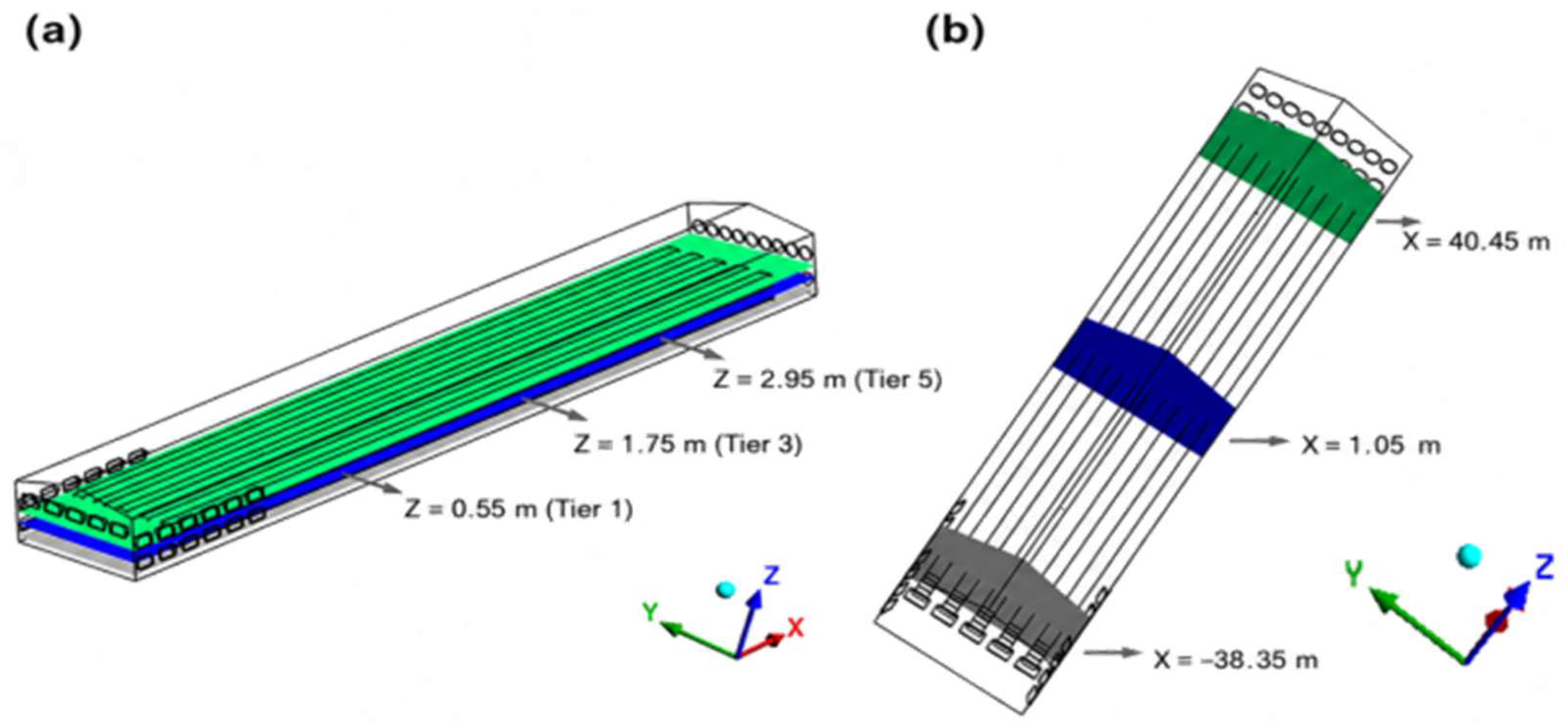
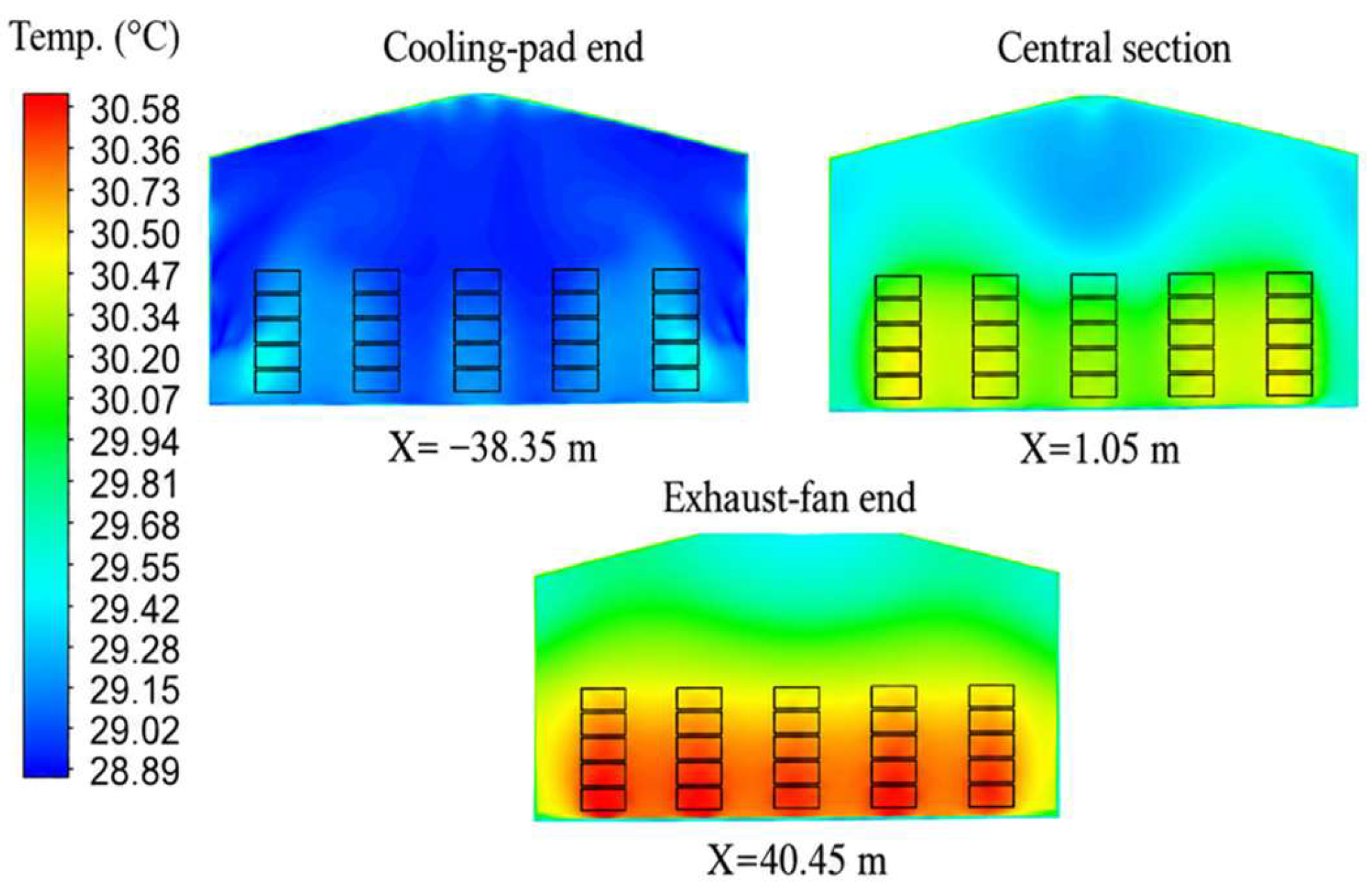
Upon convergence, the steady-state solution files generated in ANSYS Fluent 2023 R1 were imported into CFD-Post 2023 R1 for post-processing. Virtual sampling points were defined at coordinates corresponding exactly to the field monitoring locations. The simulated air temperature, relative humidity, and air velocity at each sampling point and measurement period were extracted and compared with the corresponding field measurements to assess the predictive accuracy and reliability of the CFD model. Comparisons between the simulated and measured values are presented in Figure 8, Figure 9 and Figure 10.

The calculated MRE and NMSE values are summarized in

Table 5. Error analysis of simulated and average measured values.

		Air Temperature		Relative Humidity		Air Velocity
Cage Tier	Period	MRE	NMSE	MRE	NMSE	MRE	NMSE
First layer	morning	1.30%	0.000181	2.25%	0.000656	11.09%	0.01715
	noon	1.29%	0.000165	2.96%	0.000758	11.79%	0.01997
	evening	1.36%	0.000177	2.54%	0.000681	11.60%	0.01547
Second layer	morning	1.81%	0.00042	2.51%	0.00085	9.20%	0.01022
	noon	1.10%	0.00017	1.98%	0.00054	12.44%	0.01853
	evening	1.44%	0.0003	1.91%	0.00053	11.98%	0.02103

. The MRE for air temperature and relative humidity were below 3%, whereas the maximum MRE for air velocity was 12.4%. The comparatively higher air-velocity MRE was mainly attributable to the low magnitude of the measured velocities, for which small absolute deviations resulted in relatively large percentage errors. Nevertheless, over the measured air-velocity range of 0.8–2.4 m/s, the maximum absolute deviation between the simulated and measured values was only 0.10 m/s. Moreover, the NMSE values for air temperature, relative humidity, and air velocity were all below the acceptance threshold of 0.25. These results indicate that the CFD model adequately reproduced the measured thermal, moisture, and airflow conditions and was therefore considered suitable for the subsequent analysis and optimization of the ventilation system.

3. Results and Discussion

3.1. Environmental Analysis Planes

Representative analysis planes were defined to characterize the spatial distributions of air temperature, relative humidity, and air velocity within the laying hen house. Three horizontal planes were established at Z = 0.55, 1.75, and 2.95 m, and three transverse vertical planes were defined at X = −38.35, 1.05, and 40.45 m, representing the cooling-pad end, central section, and fan end, respectively. Their locations are shown in Figure 11.

The midday simulation was selected for environmental-field analysis, corresponding to the period when the indoor temperature of the laying hen house reached its daily peak. Temperature, relative humidity, and air-velocity fields were extracted on each analysis plane and presented as spatial contour maps.

3.2. Temperature Field Simulation Results

The temperature contours on the transverse planes normal to the X-axis (Figure 12) reveal pronounced vertical thermal stratification. Heat accumulated within the cage zone, where temperatures were higher than those in the space above the cages. Along the longitudinal X-direction, air temperature increased progressively toward the fan end, resulting in a marked temperature difference between the cooling-pad end and the fan end. This pattern occurred because the cool incoming air was directed upward by the air-inlet deflectors and traveled primarily through the upper space of the house. Consequently, insufficient mixing and heat exchange occurred between the incoming airflow and the hens within the cage zone, and much of the air was exhausted through the space above and along both sides of the cages.

The vertical temperature distribution along the Z-axis is shown in Figure 13. Along the longitudinal X-direction, the temperature within the cage zone increased progressively from the cooling-pad end toward the fan end. In contrast, temperature decreased with increasing height, with the uppermost cage tier near the fan end exhibiting relatively low temperatures. This pattern resulted from the downward movement of cooled air from the upper space into the cage zone. The airflow first exchanged heat with the hens in the uppermost tier and subsequently absorbed additional metabolic heat as it penetrated downward through the cages. Consequently, the air temperature increased, and its cooling capacity progressively diminished, leading to pronounced heat accumulation in the lower cage tiers near the fan end. Comparable longitudinal and cage-dependent thermal heterogeneity was reported by Tong et al. [35], who found that spatial variation in a commercial tunnel-ventilated layer house exposed hens in different cages to unequal heat-stress risks. However, their study primarily diagnosed the thermal environment under the existing ventilation operation, whereas the present analysis identifies the airflow pathway responsible for lower-tier heat accumulation and provides a mechanistic basis for the subsequent inlet-layout optimization. This comparison demonstrates that whole-house or aisle-level averages alone are insufficient for evaluating thermal exposure in multi-tier housing.

3.3. Relative Humidity Field Simulation Results

The relative-humidity contours on the transverse planes normal to the X-axis (Figure 14) show higher relative humidity near the cooling-pad end because the cooled inlet air had a high moisture content. Relative humidity then decreased progressively with increasing distance from the air inlets, with the most pronounced reduction occurring near the fan end.

The relative-humidity distributions on the horizontal planes at different elevations are shown in Figure 15. As the plane height increased, the high-humidity region near the cooling-pad end expanded, while relative humidity near the fan end also increased. This pattern was governed by the height-dependent resistance to airflow imposed by the cage assemblies. At lower elevations, the densely arranged cages strongly impeded airflow, resulting in low air velocities and limited longitudinal penetration of the cool, moisture-laden inlet air, which therefore remained concentrated near the cooling-pad end. With increasing height, the obstruction caused by the cages diminished. At Z = 2.95 m, the open upper space provided the lowest flow resistance, allowing the humid inlet air to spread both laterally and farther downstream. Consequently, the high-humidity region at this elevation exhibited the largest spatial extent and the greatest longitudinal penetration. Kim et al. [36] showed that high relative humidity at an ambient temperature of 30 °C reduced feed intake and several egg-quality traits and intensified physiological stress responses in laying hens, although short-term hen-day egg production was not significantly affected. Accordingly, changes in relative humidity among the present ventilation cases were evaluated together with temperature, air velocity, and ETI rather than being treated as an isolated indicator of ventilation performance.

3.4. Air-Velocity Field Simulation Results

The air-velocity contours on the transverse planes normal to the X-axis (Figure 16) show that air velocity above the cages was substantially higher than that within the cage and aisle zones. Air velocities remained uniformly low throughout the cage zone, with no pronounced differences among cage tiers, indicating limited airflow penetration through the densely arranged cages. Most of the air entering through the cooling pads bypassed the cage zone and flowed through the upper space toward the exhaust fans, resulting in inadequate cooling and air exchange within the hen-occupied zone.

The air-velocity distributions on the horizontal planes at different elevations are shown in Figure 17. Air velocity was highest near the cooling-pad end, reaching a maximum of 2.73 m s⁻¹, and was markedly greater in the central aisle than in the two side aisles. Air velocity within both the cage and aisle zones increased progressively with elevation. This pattern occurred because the air-inlet deflectors directed the cooled inlet air toward the unobstructed upper space of the house, where flow resistance was substantially lower than within the densely arranged cage zone. Consequently, high-velocity airflow paths developed in the upper region, resulting in increasing air velocity with height.

3.5. Parameter Optimization Design

The contour plots presented above indicate that the current longitudinal ventilation system has several notable deficiencies, including insufficient air velocity near the fan end, inadequate cooling and air exchange, and pronounced heat accumulation within the cage zone. These deficiencies deteriorate the indoor environment and may adversely affect hen health and thermal comfort, highlighting the need to optimize the ventilation configuration.

Because inlet arrangement directly affects indoor airflow distribution, excessively narrow inlet spacing may cause airflow overlap near the cooling-pad end, increasing local air velocity while reducing airflow penetration toward the fan end. Conversely, excessively wide spacing may create airflow dead zones and further decrease fan-end air velocity. Therefore, the horizontal spacing between adjacent inlets on the east and west sidewalls was selected as the first experimental factor, with levels of 1.14 m (baseline), 1.5 m, and 2.0 m. The number of inlets at the cooling-pad end was selected as the second factor because the inlet airflow rate at this location influences ventilation uniformity. Two levels were considered: 24 inlets (baseline) and 32 inlets. The additional inlets had the same dimensions as the existing ones; four were added on each side, with two added to each of the upper and lower rows. The resulting six configurations were simulated using ANSYS Fluent 2023 R1. Case 1 represented the original model, and only inlet spacing and number were varied among cases, while all other model settings remained unchanged. The optimized inlet locations are illustrated in Figure 18, and the six configurations are summarized in

Table 6. Air-inlet configurations used in the optimization simulations.

Case	Lateral Spacing of Air Inlets/m	Number of Air Inlets
1 (original)	1.14	24
2	1.14	32
3	1.5	24
4	1.5	32
5	2.0	24
6	2.0	32

. Inlet-parameter schemes used in the optimization simulations.

3.6. Selection of the Air-Inlet Configuration Based on Evaluation Metrics

To accurately evaluate the uniformity of airflow distribution within the optimized laying hen house, an airflow non-uniformity coefficient was introduced to quantitatively assess the rearing environment within the optimized house. The airflow non-uniformity coefficient is expressed by Equation (11).

$$J_v={\displaystyle \frac{\sqrt{\frac{1}{n}\sum _{i=1}^n\left(v_i-v_p\right)}}{v_p}}$$

(11)

where J_v denotes the airflow non-uniformity coefficient; n is the total number of measurement points arranged in the experiment; v_i is the measured value of the environmental parameter at the ith measurement point, such as air velocity, air temperature, or relative humidity; and v_p is the mean value of the corresponding environmental parameter across all measurement points, namely the mean air velocity, mean air temperature, or mean relative humidity. The non-uniformity coefficients for the above optimization cases are presented in

Table 7. The non-uniformity coefficient of different air inlet parameters.

Case	Temperature	Relative Humidity	Air Velocity
1	0.02288	0.03003	0.44736
2	0.01876	0.02451	0.40021
3	0.02197	0.02887	0.46768
4	0.01823	0.02387	0.42768
5	0.02205	0.02900	0.46929
6	0.01778	0.02328	0.44973

.

As shown in Table 7, adjustments to both air-inlet spacing and air-inlet number affected the spatial uniformity of the key environmental parameters within the laying hen house. In this study, the non-uniformity coefficient was used as a quantitative indicator of environmental uniformity, and the two were inversely related; that is, a lower non-uniformity coefficient indicated a more uniform spatial distribution of the corresponding environmental parameter. Specifically, increasing the horizontal spacing between adjacent air inlets improved the distribution uniformity of air temperature and relative humidity but reduced the uniformity of air velocity. By contrast, increasing the number of air inlets consistently improved the distribution uniformity of air temperature, relative humidity, and air velocity. A comprehensive comparison of the six optimization cases showed that Case 6 achieved the best uniformity in air temperature and relative humidity among all cases, whereas its air-velocity uniformity showed no appreciable difference from that of the baseline Case 1. Case 2 ranked second only to Case 6 in terms of temperature and relative-humidity uniformity and exhibited the highest air-velocity uniformity among all cases.

Previous CFD studies obtained substantial environmental changes by relocating or resizing exhaust fans and cooling pads or by introducing additional airflow-guiding structures [20,21,37]. These approaches involve broader modifications to the ventilation system and are not directly comparable with the constrained retrofit examined here, in which the installed fans, cooling pads, ventilation mode, and operating conditions were retained. Within this controlled design space, Case 2 was selected because it provided the best compromise among temperature, relative-humidity, and air-velocity uniformity rather than the minimum value of any single non-uniformity coefficient. This distinction is important because Case 6 produced slightly better temperature and relative-humidity uniformity, but its air-velocity uniformity was not appreciably improved relative to the original model.

In addition, to further evaluate the overall effectiveness of the different optimization cases in regulating the indoor thermal environment, the effective temperature index (ETI) was introduced as an integrated thermal-environment assessment metric. This index was developed using linear regression based on three key environmental parameters—air temperature, relative humidity, and air velocity—and integrates their combined effects on the quality of the rearing environment within the laying hen house. The equations for calculating the effective temperature index for laying hens, developed by Bjerg et al. [38,39] through linear regression analysis, are presented in Equations (12) and (13).

$$\mathrm{ETI}=\left(0.794{\mathrm{t}}_{\mathrm{d}}+0.25{\mathrm{t}}_{\mathrm{w}}+0.7\right) -0.15 \text{×} \left(44- {\mathrm{t}}_{\mathrm{d}}\right) \text{×} \left({\mathrm{v}}^{0.5} {- 0.2}^{0.5}\right)$$

(12)

$${\mathrm{t}}_{\mathrm{w}}=0.85569{\mathrm{t}}_{\mathrm{d}}+0.178 02\mathrm{RH} - 12.35087$$

(13)

where t_d is the dry-bulb temperature (°C), t_w is the wet-bulb temperature (°C), and v is the air velocity (m/s⁻¹).

The four core input parameters required for ETI calculation—dry-bulb temperature, wet-bulb temperature, relative humidity, and air velocity—were all derived from the CFD numerical simulation results and subjected to standardized post-processing and parameter extraction using ANSYS CFD-Post 2023 R1. The parameters were obtained as follows. The underlying dry-bulb temperature and air-velocity data were taken directly from the simulated temperature and velocity fields generated after numerical solution in the Fluent Solution module. Relative humidity was calculated based on the thermodynamic relationship between the water-vapor mass fraction and the temperature field of the indoor air. Wet-bulb temperature was then calculated by substituting the obtained dry-bulb temperature and relative humidity into Equation (13). After all the above input parameters had been extracted, batch post-processing calculations of ETI were performed using the built-in user-defined expression function in ANSYS CFD-Post 2023 R1, followed by standardized data export. Based on this calculation procedure, the calculated mean ETI values within the cage zone for all the above optimization cases are presented in Figure 19.

As indicated by the mean perceived temperatures in the cage zone presented in Figure 19, the effectiveness of the different air-inlet parameter configurations in regulating the perceived temperature within the laying hen house varied. The mean perceived temperatures under Cases 1, 3, and 5 were 27.40, 27.30, and 27.44 °C, respectively, whereas those under Cases 2, 4, and 6 were only 26.90, 26.87, and 26.89 °C, respectively. Overall, Cases 2, 4, and 6 not only markedly reduced the mean perceived temperature within the house but also resulted in smaller differences among the cage tiers. These results indicate that, under these three configurations, the thermal environment within the laying hen house was more uniformly distributed in space, thereby providing more favorable thermal comfort conditions for the laying hens. Because ETI integrates the combined effects of air temperature, relative humidity, and air velocity, the lower values obtained for the 32-inlet configurations indicate an overall reduction in thermal load rather than an improvement in only one environmental variable [38,39].

3.7. Comparison Between the Optimized and Original Configurations

To accurately evaluate the optimization performance of the proposed Case 2, a comprehensive comparative analysis was conducted on the spatial distributions of air temperature, relative humidity, and air velocity within the laying hen house under the baseline configuration and Case 2. To eliminate the potential influence of differences in the analysis planes on the comparison results, all three environmental fields were evaluated on the same horizontal plane at a height of 1.75 m above the floor of the laying hen house.

3.7.1. Analysis of Temperature-Field Optimization

The temperature-field contours for the two ventilation configurations are compared in Figure 20. Under the original model, the air temperature within the laying hen house exhibited a pronounced longitudinal increase, rising progressively from the cooling-pad end toward the fan end. A distinct local high-temperature region developed near the air-outlet side, indicating substantial heat accumulation. The regional peak temperature reached approximately 31 °C, and the high-temperature region covered a relatively large area, resulting in pronounced spatial non-uniformity of the indoor temperature field. Following optimization under Case 2, the spatial uniformity of the temperature field was improved, and the overall temperature distribution became more uniform. The peak temperature decreased to 30.5 °C, while both the maximum temperature and the spatial extent of the high-temperature region were markedly reduced. Consequently, heat accumulation near the downstream end of the house was effectively alleviated, which may reduce heat-stress responses in laying hens and improve the suitability of the indoor thermal environment.

3.7.2. Comparative Analysis of the Relative-Humidity Field

The relative-humidity contour plots for the two ventilation schemes are compared in Figure 21. In the original model, the peak relative humidity in the air-inlet region was approximately 87%. However, relative humidity decreased rapidly and substantially along the airflow direction, exhibiting an overall linear decline from the cooling-pad end to the fan end. Green-to-blue regions appeared near the air-outlet end, indicating a marked reduction in relative humidity and pronounced spatial variation in the humidity field. Although this distribution pattern provided relatively high moisture-removal efficiency, it could not ensure a uniform humidity environment within the laying hen house. In comparison, under Case 2, the longitudinal decrease in relative humidity was more gradual, and the spatial uniformity of the relative-humidity field was substantially improved. Only a slight increase in relative humidity occurred near the downstream end of the house. Although the overall moisture-removal capacity was slightly lower than that of the original model, Case 2 showed clear advantages in the stability and uniformity of the humidity distribution, thereby providing a more stable humidity environment for laying hens.

3.7.3. Comparative Analysis of the Air-Velocity Field

The air-velocity contour plots for the two ventilation schemes are compared in Figure 22. In the original model, an extensive low-velocity dead zone developed near the fan end of the laying hen house, and the overall air-velocity distribution was highly non-uniform. Airflow circulation and air-exchange efficiency were insufficient in the downstream section of the cage zone. The calculated air-velocity non-uniformity coefficient reached 0.44736, directly indicating pronounced spatial variation in air velocity throughout the house. Following optimization under Case 2, air velocity near the fan end increased markedly, the spatial extent of the low-velocity regions was substantially reduced, and the airflow paths became more concentrated and orderly. Consequently, the overall air-velocity non-uniformity coefficient decreased to 0.40021, indicating a marked improvement in ventilation uniformity within the house. These results demonstrate that Case 2 effectively enhanced ventilation and air-exchange efficiency within the cage zone, produced a more rational indoor airflow pattern, and substantially alleviated the excessively extensive low-velocity regions observed in the original model.

3.7.4. Comparative Analysis of the Perceived-Temperature Field

The perceived-temperature contour plots for the two ventilation schemes are compared in Figure 23. In the original model, the perceived temperature exhibited a gradual increasing trend along the length of the laying hen house, with pronounced accumulation of high perceived temperatures in the end region, where the maximum perceived temperature approached 28.36 °C.

3.7.5. Analysis of the Thermal Environment in the Cage Zone

The comparisons of mean air temperature, mean air velocity, and mean relative humidity within the cage zone under the original operating condition and Case 2 are presented in Figure 24. Under the original operating condition, air velocities across cage tiers 1–4 were relatively low, whereas the air velocity at the top cage tier was higher, reaching 0.9 m/s. The mean air temperature at all five cage tiers exceeded 30 °C, indicating poor overall environmental uniformity within the cage zone. Following airflow-field optimization, air velocity increased markedly across all cage tiers, with the maximum value reaching 1.1 m/s. The mean air temperature within the cage zone decreased by up to 0.4 °C, corresponding to a reduction of 1.32%, and remained below 30 °C at all cage tiers. The mean relative humidity within the cage zone increased slightly; however, this increase was not sufficient to adversely affect the productive performance of the laying hens.

Previous studies have shown that, within the temperature range of 25–30 °C, each 1 °C increase in ambient temperature results in a 1.5% relative decrease in the egg production rate. Once the temperature exceeds 30 °C, the decline in egg production becomes substantially more pronounced. For example, at 32 °C, the egg production rate is 7.4% lower than that at 21 °C, indicating that 30 °C represents a critical inflection point beyond which egg production declines sharply [40,41]. The 0.4 °C temperature reduction achieved through the present optimization lowered the cage-zone temperature from above 30 °C, a high-risk range associated with a sharp decline in egg production, to the approximately linear-response range of 25–30 °C, thereby avoiding the risk of temperature-induced deterioration in laying performance. Based on the reported temperature response of egg production within the 25–30 °C range, the 0.4 °C reduction corresponds to a theoretical direct increase of 0.6% in the egg production rate. For a flock of 48,000 laying hens with a baseline egg production rate of 90%, this improvement would yield more than 90,000 additional eggs annually. When the additional benefits associated with improved egg quality and feed-to-egg ratio are also considered, the overall economic benefit to laying-hen production would be substantial.

4. Conclusions

This study developed and validated a CFD model for a commercial five-tier stacked-cage laying hen house under summer tunnel-ventilation conditions. Field measurements of air temperature, relative humidity, air velocity, and structural parameters were used to establish the whole-house model and the porous-medium model of the cage-and-hen occupied zone. The main conclusions are as follows:

(1)

The CFD model reproduced the measured thermal and airflow environment with acceptable accuracy. The mean relative errors (MREs) for air temperature and relative humidity were below 3%, while the MREs for air velocity were approximately 10%. All normalized mean square error (NMSE) values were below 0.25, indicating that the model was sufficiently reliable for analyzing the indoor environmental distribution and evaluating alternative ventilation-optimization schemes.

(2)

Under the original ventilation configuration, heat accumulated in the middle and downstream sections of the laying hen house, where local air temperatures exceeded 31 °C. Relative humidity was highest near the cooling-pad inlet and decreased progressively toward the fan end. The airflow field was also unevenly distributed. Air velocity reached approximately 2.42 m s⁻¹ near the inlet and along the upper airflow path but decreased to approximately 0.8–1.0 m s⁻¹ in the middle and downstream cage regions. These results indicate that a substantial proportion of the cooled inlet air flowed through the open space above the cages, whereas effective airflow delivery to the cage zone remained insufficient.

(3)

Coordinated adjustment of air-inlet number and horizontal spacing improved the spatial uniformity of air temperature, relative humidity, and air velocity. Among the six configurations evaluated, the preferred scheme maintained a horizontal inlet spacing of 1.14 m and increased the total number of air inlets at the cooling-pad ends of the two sidewalls from 24 to 32. Compared with the original configuration, this scheme reduced the non-uniformity coefficients of air temperature, relative humidity, and air velocity by 18.00%, 18.38%, and 10.54%, respectively, while decreasing the mean effective temperature index in the cage zone by 0.5 °C. Air velocity increased across all five cage tiers, and the mean air temperature at each tier was reduced to below 30 °C. Therefore, the preferred inlet configuration provided the most balanced improvement in the thermal and airflow environment among the investigated schemes.

The present analysis focused on the measured summer operating conditions and the investigated range of air-inlet configurations. Future studies should implement the preferred configuration in a commercial laying hen house and evaluate its performance under different outdoor climatic conditions, ventilation rates, and fan operating states. Transient and multi-season simulations, combined with long-term field monitoring of energy consumption, hen physiological responses, production performance, and egg quality, would further determine the comprehensive benefits of the proposed ventilation modification.

Overall, the validated CFD model and preferred air-inlet configuration provide a practical basis for improving summer ventilation uniformity and mitigating localized heat accumulation in high-density multi-tier laying hen houses.