Author Contributions
Conceptualization, B.J., C.L. and L.F.; Methodology, B.J., J.Z., R.L., M.Y. and S.H.L.; Software, J.Z.; Validation, S.K., J.H. and X.M.; Formal analysis, B.J.; Investigation, B.J. and S.K.; Data curation, B.J., S.K., J.H. and X.M.; Writing—original draft preparation, B.J.; Writing—review and editing, J.Z., C.L. and L.F.; Supervision, C.L. and L.F.; Funding acquisition, R.L. and L.F. All authors have read and agreed to the published version of the manuscript.
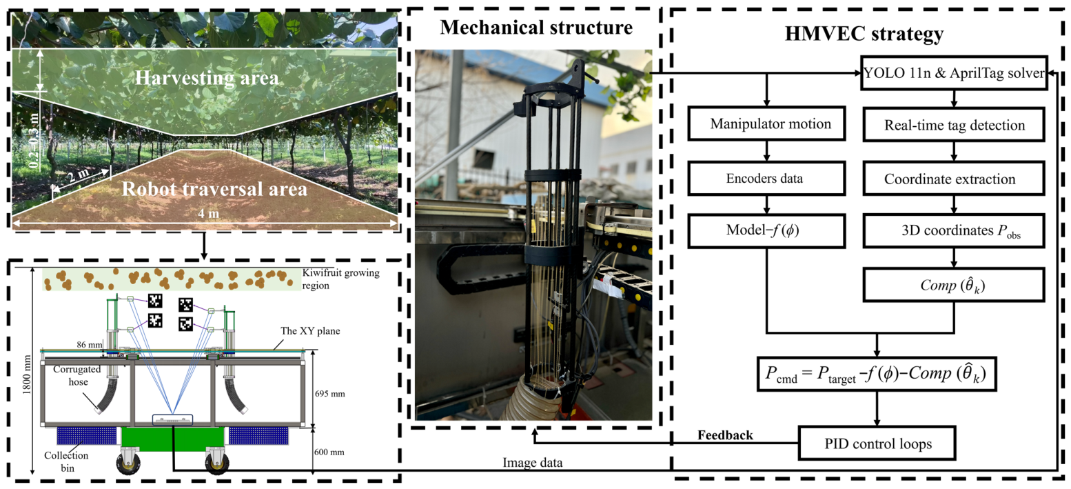
Figure 1.
Overall architecture of the telescopic manipulator system for terminal positioning-error compensation and post-detachment fruit transfer in trellis-grown kiwifruit harvesting. The top-left panel illustrates the spatial constraints of the standardized kiwifruit trellis environment. The bottom-left schematic details the hardware integration, including the mobile platform and the binocular stereo vision system. The central photograph displays the physical prototype of the hollow telescopic manipulator. The right panel presents the control flowchart of the hybrid model–vision error compensation (HMVEC) strategy.
Figure 1.
Overall architecture of the telescopic manipulator system for terminal positioning-error compensation and post-detachment fruit transfer in trellis-grown kiwifruit harvesting. The top-left panel illustrates the spatial constraints of the standardized kiwifruit trellis environment. The bottom-left schematic details the hardware integration, including the mobile platform and the binocular stereo vision system. The central photograph displays the physical prototype of the hollow telescopic manipulator. The right panel presents the control flowchart of the hybrid model–vision error compensation (HMVEC) strategy.
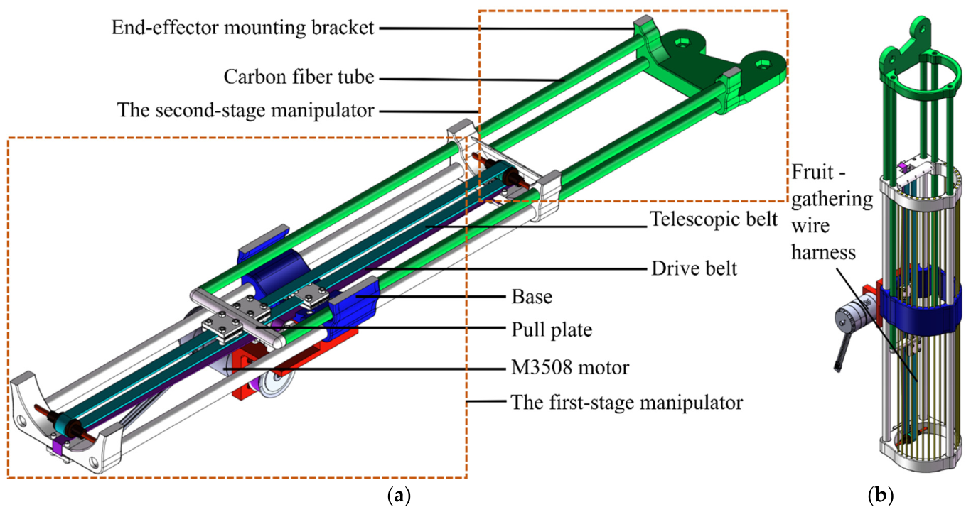
Figure 2.
Hollow telescopic manipulator design. (a) Belt-driven cascaded mechanism with labeled components. The drive belt extends the first-stage manipulator while the constrained telescopic belt simultaneously extends the second-stage manipulator, achieving 1.83:1 kinematic ratio. (b) Overall structure of the telescopic manipulator.
Figure 2.
Hollow telescopic manipulator design. (a) Belt-driven cascaded mechanism with labeled components. The drive belt extends the first-stage manipulator while the constrained telescopic belt simultaneously extends the second-stage manipulator, achieving 1.83:1 kinematic ratio. (b) Overall structure of the telescopic manipulator.
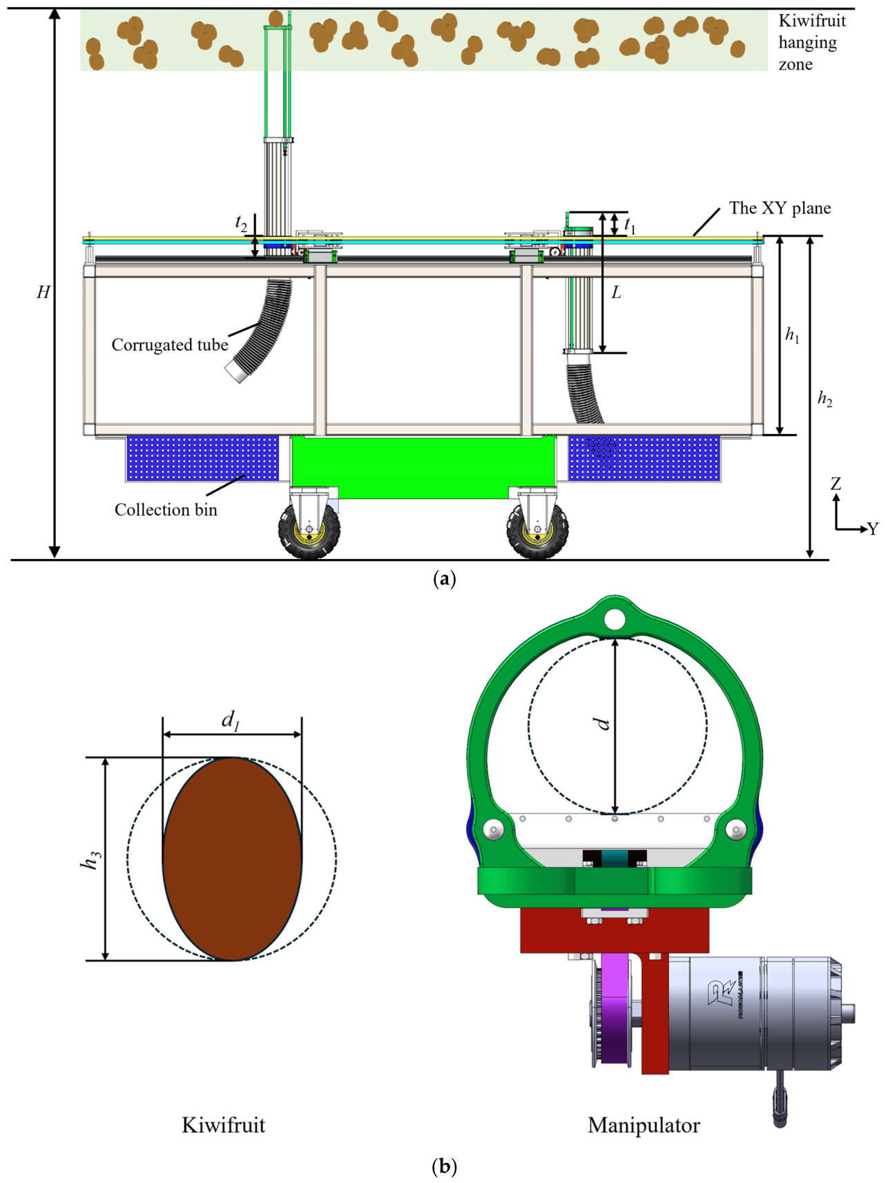
Figure 3.
Dimensional design and spatial constraint analysis of the telescopic manipulator. (a) Vertical spatial constraints of the Cartesian mechanism operating under the kiwifruit hanging zone. (b) Dimensional matching between kiwifruit geometric parameters and the hollow manipulator.
Figure 3.
Dimensional design and spatial constraint analysis of the telescopic manipulator. (a) Vertical spatial constraints of the Cartesian mechanism operating under the kiwifruit hanging zone. (b) Dimensional matching between kiwifruit geometric parameters and the hollow manipulator.
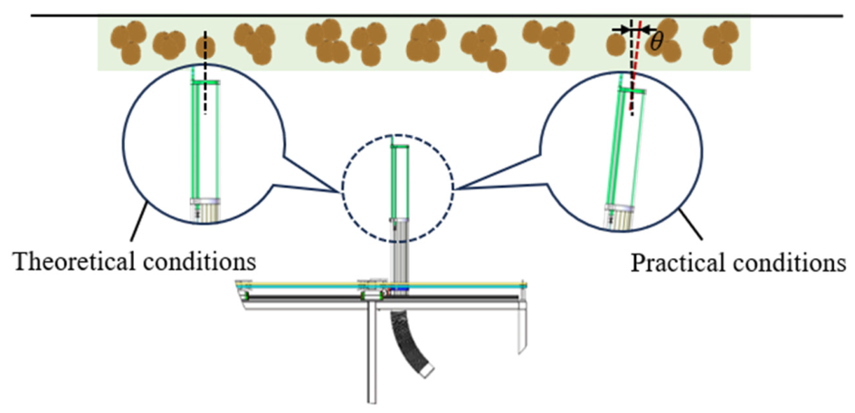
Figure 4.
Structural deflection of the telescopic manipulator during vertical extension. The left side displays the theoretical conditions with perfect vertical alignment. The right side illustrates the practical conditions. The symbol θ denotes the actual deflection angle caused by structural bending.
Figure 4.
Structural deflection of the telescopic manipulator during vertical extension. The left side displays the theoretical conditions with perfect vertical alignment. The right side illustrates the practical conditions. The symbol θ denotes the actual deflection angle caused by structural bending.
Figure 5.
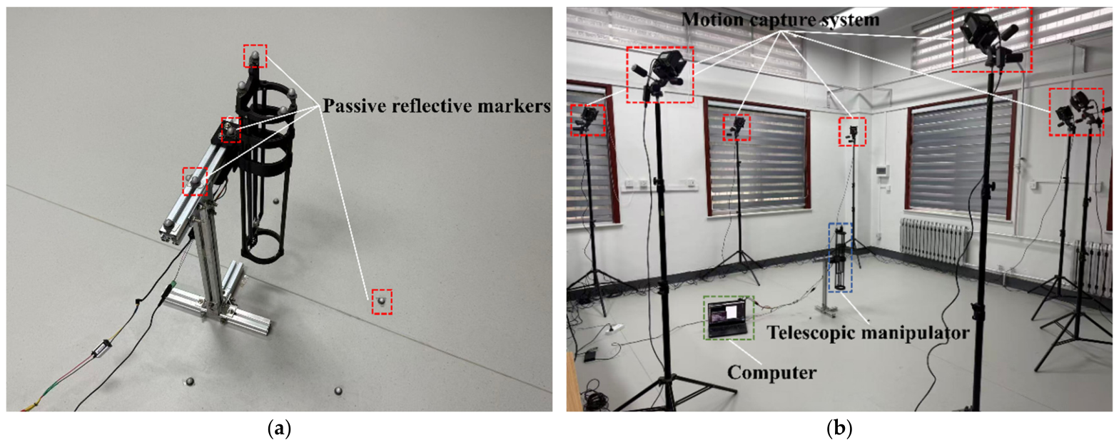
Experimental setup for kinematic trajectory acquisition. (a) The telescopic manipulator instrumented with passive reflective markers for pose tracking. (b) Global layout of the Mars 1.3H optical motion capture system environment, the system consists of a host computer, a telescopic manipulator, and seven optical cameras.
Figure 5.
Experimental setup for kinematic trajectory acquisition. (a) The telescopic manipulator instrumented with passive reflective markers for pose tracking. (b) Global layout of the Mars 1.3H optical motion capture system environment, the system consists of a host computer, a telescopic manipulator, and seven optical cameras.
Figure 6.
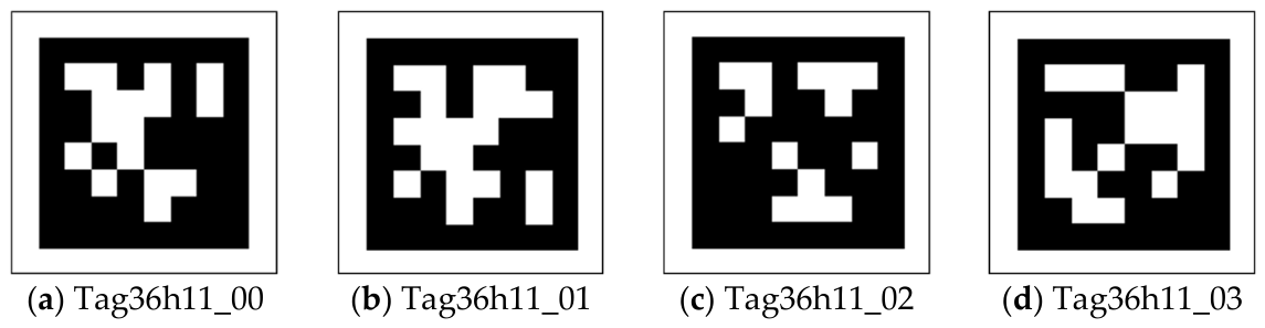
The four types of AprilTag markers used in this experimental.
Figure 6.
The four types of AprilTag markers used in this experimental.
Figure 7.
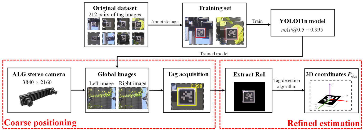
Two-stage detection module workflow. YOLO11n detection was used to acquire the RoI while the AprilTag detection processed the extracted tag pair to estimate the refined position.
Figure 7.
Two-stage detection module workflow. YOLO11n detection was used to acquire the RoI while the AprilTag detection processed the extracted tag pair to estimate the refined position.
Figure 8.
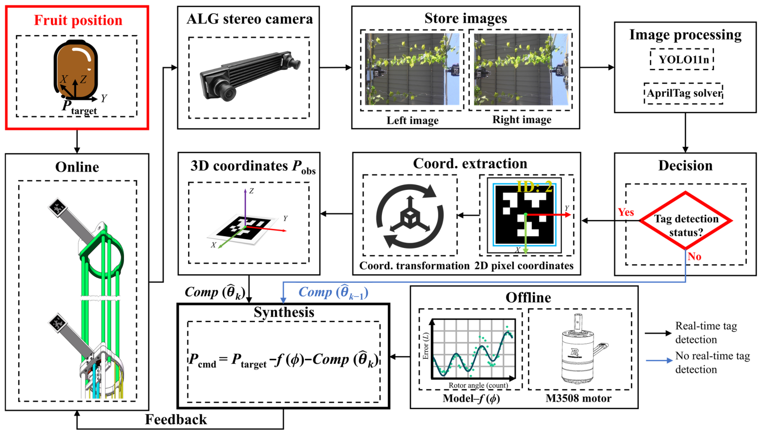
The proposed hybrid adaptive control architecture. It integrates an offline polynomial–Fourier feedforward model for static error compensation and a real-time visual feedback loop driven by YOLO11n and AprilTag methods to handle dynamic disturbances.
Figure 8.
The proposed hybrid adaptive control architecture. It integrates an offline polynomial–Fourier feedforward model for static error compensation and a real-time visual feedback loop driven by YOLO11n and AprilTag methods to handle dynamic disturbances.
Figure 9.
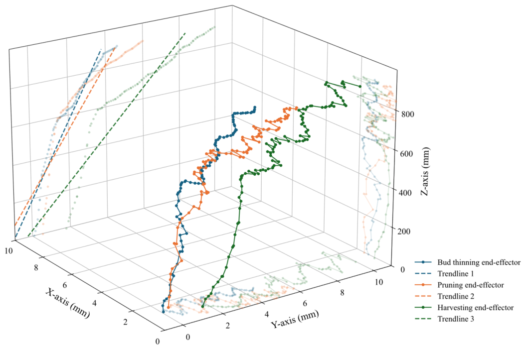
Three-dimensional motion trajectories of the telescopic manipulator during the extension process under varying end-effector loads. For each payload condition, the displayed trajectory was obtained by aligning 20 complete motion trajectories according to the motor encoder counts and averaging the X, Y, and Z axes displacements at identical encoder-count positions. Deviations along the X-axis indicate lateral instability, while deviations along the Y-axis reflect gravity-induced bending under different payload conditions.
Figure 9.
Three-dimensional motion trajectories of the telescopic manipulator during the extension process under varying end-effector loads. For each payload condition, the displayed trajectory was obtained by aligning 20 complete motion trajectories according to the motor encoder counts and averaging the X, Y, and Z axes displacements at identical encoder-count positions. Deviations along the X-axis indicate lateral instability, while deviations along the Y-axis reflect gravity-induced bending under different payload conditions.
Figure 10.
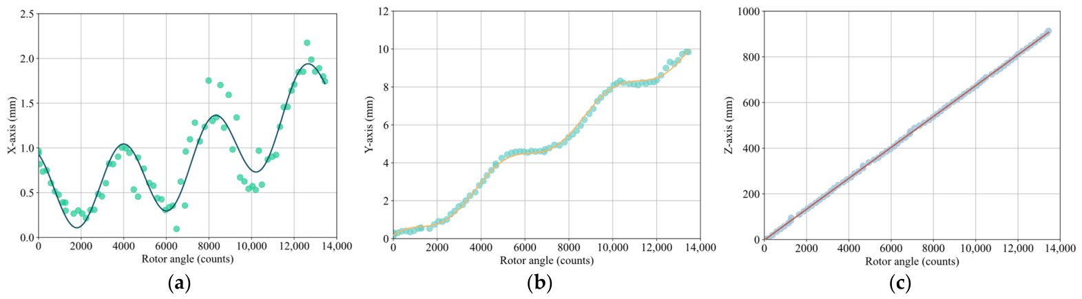
Regression analysis of the relationship between the 3D pose of the harvesting manipulator’s end-effector and the motor rotor angle. (a) X-axis displacement, showing the lateral oscillation trend and the fitted polynomial–Fourier curve; (b) Y-axis displacement, showing the nonlinear deflection trend mainly caused by gravitational loading and the fitted polynomial–Fourier curve; and (c) Z-axis displacement, showing the approximately linear extension trend and the fitted linear curve.
Figure 10.
Regression analysis of the relationship between the 3D pose of the harvesting manipulator’s end-effector and the motor rotor angle. (a) X-axis displacement, showing the lateral oscillation trend and the fitted polynomial–Fourier curve; (b) Y-axis displacement, showing the nonlinear deflection trend mainly caused by gravitational loading and the fitted polynomial–Fourier curve; and (c) Z-axis displacement, showing the approximately linear extension trend and the fitted linear curve.
Figure 11.
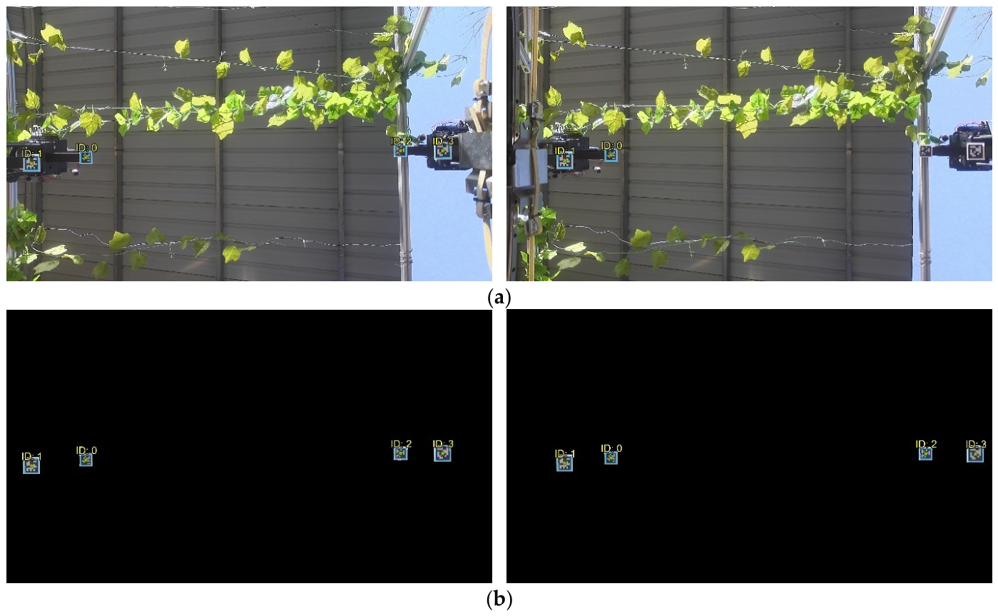
Comparative evaluation of AprilTag detection performance. (a) Traditional direct tag detection methods. (b) The proposed coarse-to-fine detection method. This strategy integrates the YOLO11n model for initial RoI extraction (coarse), followed by precise tag localization within the cropped bounding box (fine).
Figure 11.
Comparative evaluation of AprilTag detection performance. (a) Traditional direct tag detection methods. (b) The proposed coarse-to-fine detection method. This strategy integrates the YOLO11n model for initial RoI extraction (coarse), followed by precise tag localization within the cropped bounding box (fine).
Figure 12.
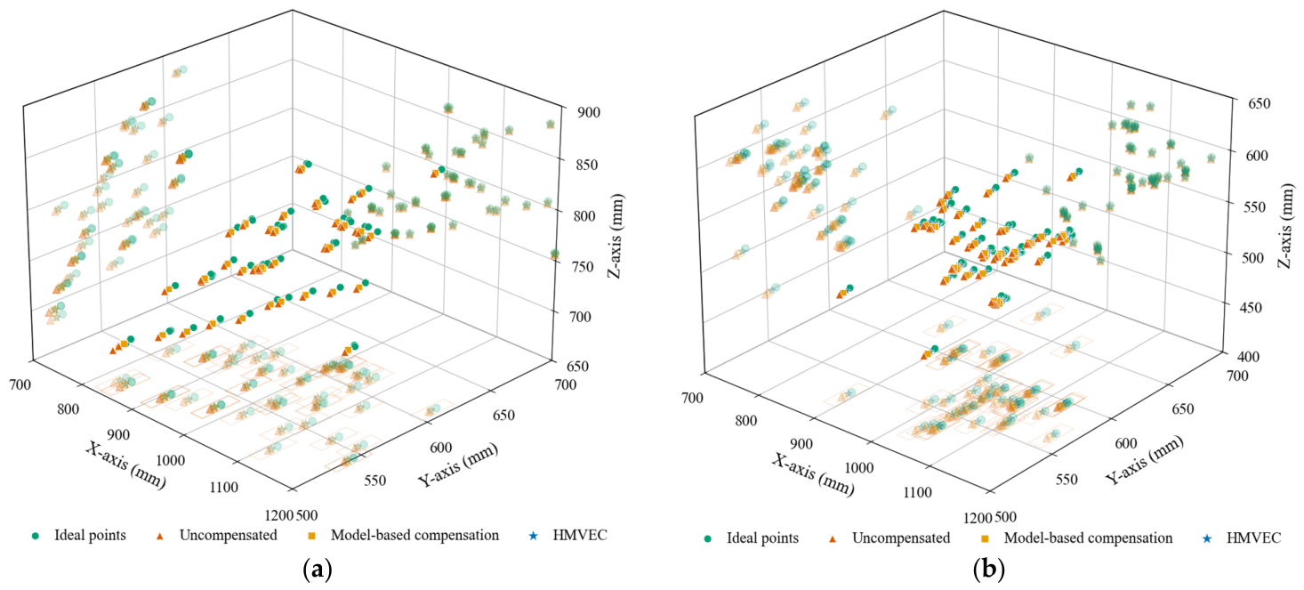
Comparison of 3D trajectories of the manipulator end point under different compensation strategies for the (a) left and (b) right manipulators.
Figure 12.
Comparison of 3D trajectories of the manipulator end point under different compensation strategies for the (a) left and (b) right manipulators.
Figure 13.
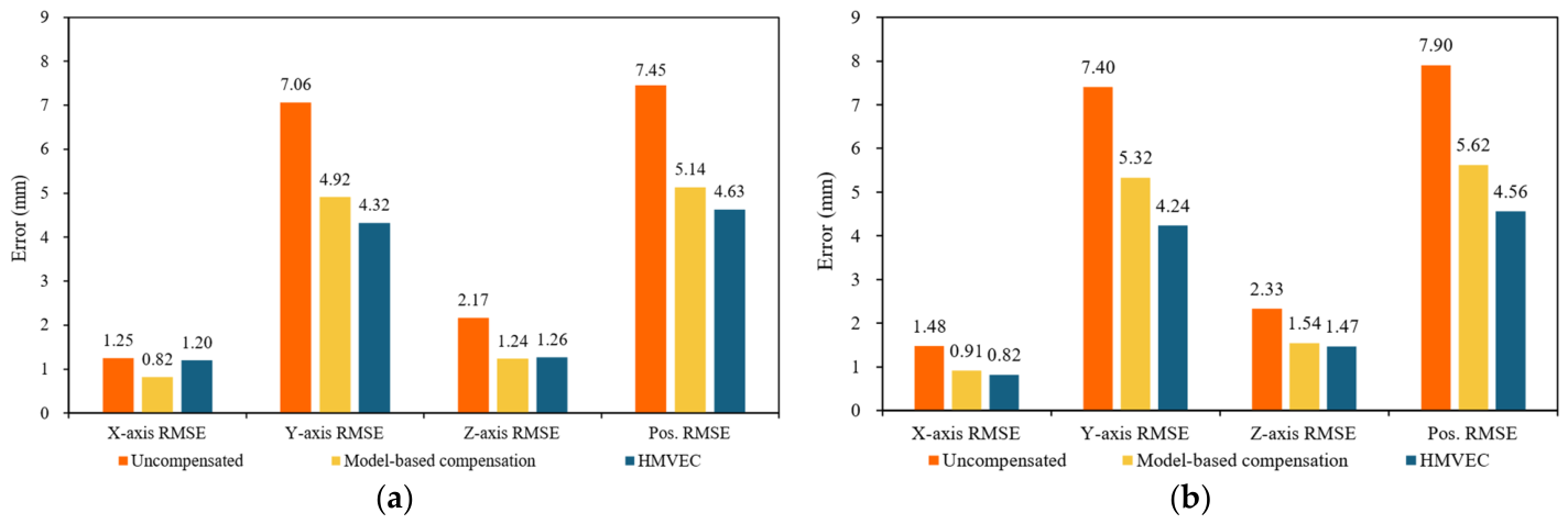
RMSE-based comparative analysis of positioning accuracy under different compensation strategies for the (a) left and (b) right manipulators, illustrating both individual-axis errors and overall positioning error.
Figure 13.
RMSE-based comparative analysis of positioning accuracy under different compensation strategies for the (a) left and (b) right manipulators, illustrating both individual-axis errors and overall positioning error.
Figure 14.
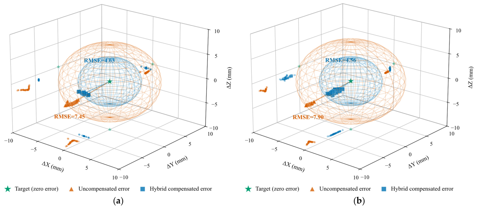
Three-dimensional distributions of positioning errors of the (a) left and (b) right manipulators under uncompensated and hybrid predictive compensated conditions, where RMSE spheres represent the overall error magnitude and visualize the reduction of positioning errors after compensation.
Figure 14.
Three-dimensional distributions of positioning errors of the (a) left and (b) right manipulators under uncompensated and hybrid predictive compensated conditions, where RMSE spheres represent the overall error magnitude and visualize the reduction of positioning errors after compensation.
Table 1.
Technical specifications of the dual-manipulator kiwifruit production platform and geometric dimensions of kiwifruit.
Table 1.
Technical specifications of the dual-manipulator kiwifruit production platform and geometric dimensions of kiwifruit.
| | Dual-Manipulator Kiwifruit Production Platform | Kiwifruit |
|---|
| Parameter | λ | H | h1 | h2 | t1 | t2 | h3 | d1 |
| Dimension | 1.83 | 1800 mm | 695 mm | 1295 mm | 80 mm | 86 mm | 100 mm | 80 mm |
Table 2.
Specifications of the platform for YOLO11n model training and deployment.
Table 2.
Specifications of the platform for YOLO11n model training and deployment.
| Item | Details |
|---|
| CPU | Intel Core i5-13600KF |
| GPU | Nvidia GeForce RTX 4060 (8 GB) |
| Memory Size | 32 GB |
| OS | Microsoft Windows 10 (64-bit) |
| Python Version | 3.10.19 |
| PyTorch Version | 2.3.1 |
| CUDA Version | 11.8 |
Table 3.
Polynomial–Fourier regression models and coefficients of determination fitted from the fused mean trajectory of 20 calibration trials under the harvesting end-effector condition.
Table 3.
Polynomial–Fourier regression models and coefficients of determination fitted from the fused mean trajectory of 20 calibration trials under the harvesting end-effector condition.
| Axis | Regression Models | R2 |
|---|
| X | y = 6.892 × 10−9x2 − 9.792 × 10⁻⁶x + 0.435sin (1.473 × 10⁻³x + 2.040) + 0.539 | 0.896 |
| Y | y = −1.303 × 10−9x2 + 7.930 × 10⁻⁴x + 0.545sin (1.270 × 10⁻³x + 1.533) − 0.370 | 0.998 |
| Z | y = 0.068x − 2.422 | 0.999 |
Table 4.
Axis-wise approximation errors of the regression models within the operating range.
Table 4.
Axis-wise approximation errors of the regression models within the operating range.
| Axis | Mean Error/mm | Median Error/mm | Maximum Error/mm |
|---|
| X | 0.123 | 0.079 | 0.441 |
| Y | 0.109 | 0.013 | 0.423 |
| Z | 2.699 | 2.599 | 7.157 |
Table 5.
Performance metrics of YOLO11n AprilTag marker detection.
Table 5.
Performance metrics of YOLO11n AprilTag marker detection.
| Metric | Value |
|---|
| Training image pairs | 212 |
| Validation image pairs | 53 |
| Precision | 1 |
| Recall | 0.9953 |
| F1-score | 0.9976 |
| mAP0.5 | 0.9950 |
| mAP0.5:0.95 | 0.9439 |
| Inference time | 3.8 ms/image |
| Tag size | 40 × 40 mm |
Table 6.
Quantitative comparison of tag detection performance between the traditional method and the proposed YOLO11n integrated method.
Table 6.
Quantitative comparison of tag detection performance between the traditional method and the proposed YOLO11n integrated method.
| | Left Camera | Right Camera | Combined Total | Detection Rate |
|---|
| Traditional method | 190 | 153 | 343 | 80.90% |
| YOLO11n | 212 | 210 | 422 | 99.53% |
Table 7.
Comparison of the proposed HMVEC strategy with representative visual feedback compensation methods.
Table 7.
Comparison of the proposed HMVEC strategy with representative visual feedback compensation methods.
| Method | Main Features | Strengths | Weaknesses |
|---|
| Singh et al. [29] | Deep-learning-based perception and MoveIt-based motion planning | Strong 3D perception and planning capability | Mainly relies on rigid-body kinematics; does not explicitly model structural deformation of telescopic manipulators |
| Chang et al. [30] | Two-stage fuzzy logic control based on visual feedback | Does not require an explicit physical model; can compensate for visual tracking deviations | Heuristic control rules; may be sensitive to occlusion and lacks explicit compensation for gravity-induced deformation |
| Proposed HMVEC strategy | Polynomial–Fourier feedforward model + YOLO11n-assisted AprilTag tracking + Hold Strategy | Compensates systematic structural deformation and reduces residual positioning errors; maintains compensation during temporary visual interruption | Currently depends on artificial AprilTag markers and was validated under simulated orchard conditions |




 ,
,