Calibration and Experimental Validation of Discrete Element Model Parameters for Cotton Stalks and Cotton Residues Mixture

Abstract

Accurate discrete element simulation parameters for the mechanically harvested cotton stalks and cotton residues mixture are currently unavailable. This lack hinders the effective design and optimization of equipment for separating and recovering cotton residues from the mixture. This study focused on the cotton stalks and cotton residues mixture. The intrinsic parameters of cotton residues were measured through physical experiments. Using the inclined plane and collision methods, the coefficients of restitution for cotton residues–cotton stalks and cotton residues–steel were determined to be 0.228 and 0.364, respectively. The corresponding static friction coefficients were 0.632 and 0.266, and the rolling friction coefficients were 0.199 and 0.156. The Hertz–Mindlin with JKR contact model was employed. Combined with repose angle tests, the coefficient of restitution, rolling friction coefficient, static friction coefficient, and surface energy for cotton residues–cotton residues were calibrated as 0.393, 0.140, 0.742, and 1.471 J/m², respectively. A vibrating spreading test was conducted to validate the calibrated parameters. The proportion of cotton residues on the material surface was used as the test index. The mean relative error between simulation and physical test results under four working conditions was 4.91%. The results indicate that acceptable consistency is achieved between simulation and experimental results under the tested conditions, and the calibrated discrete element parameters are applicable for the simulation of cotton stalk–cotton residue mixture systems. This study provides a theoretical basis and data support for the development of equipment to separate and recover cotton residues from cotton stalk and cotton residue mixtures.

1. Introduction

Cotton is one of the most important economic crops worldwide. Cotton stalks are a major by-product of cotton production. The global cotton planting area reaches 3.192 × 10⁷ ha. The global annual output of cotton stalks reaches 9.03 × 10⁷ t, indicating abundant cotton stalk resources [1,2]. Cotton stalks are agricultural biomass resources with great development potential. In their diversified high-value utilization systems for fuel, feed, fertilizer, substrate, and raw material applications, the efficient removal of cotton residues entrained in cotton stalks is a critical pre-process for subsequent resource conversion. It has fundamental and decisive significance for ensuring material quality, improving conversion efficiency, and expanding application scenarios [3,4,5,6]. Therefore, developing efficient equipment for separating and recovering cotton residues is essential to promote the green, high-value utilization of cotton stalks and reduce resource waste. This will provide clean and homogeneous raw material guarantee for the subsequent high-value conversion of cotton stalks.

Discrete element simulation technology is an effective tool for analyzing the dynamics of granular materials. It has been widely used in the field of agricultural machinery design and optimization [7,8,9]. Accurate discrete element models can reveal the movement laws and mechanical behaviors of materials under complex working conditions. They provide theoretical guidance for optimizing equipment structural parameters and matching operating parameters [10,11]. However, the cotton stalks and cotton residues mixture has complex morphology and significant differences in physical properties. Cotton residues tend to agglomerate and adhere due to electrostatic adsorption and fine fiber entanglement. This makes their contact characteristics complex and contact parameters difficult to obtain accurately through traditional physical tests [12,13,14,15]. Discrete element parameter calibration can effectively reduce the error between physical and simulation tests. Agricultural materials can be divided into non-cohesive and cohesive granular materials based on their properties. Many scholars have calibrated contact parameters for non-cohesive granular materials using the Hertz–Mindlin no slip contact model. These materials include alfalfa stalks [16], corn seeds [17,18], wheat seeds [19,20], wheat stalks [21], corn stalks [22], and rice seeds [23]. They have used the Hertz–Mindlin with JKR model for cohesive granular materials. These materials include soil [24], distiller’s grains [25], feed [26], and pig manure [27]. To date, few scholars have conducted discrete element parameter calibration and experimental research on mechanically harvested cotton stalks and cotton residues mixture from Xinjiang cotton regions.

This study takes mechanically harvested cotton stalks and cotton residues mixture as the research object. It calibrates the contact parameters between cotton residues–cotton stalks and cotton residues–steel by combining physical and simulation tests. Based on the Hertz–Mindlin with JKR contact model, the steepest ascent and Box–Behnken test methods were used. The angle of repose was taken as the response value to calibrate the cohesive contact parameters between cotton residues–cotton residues. Finally, a vibratory spreading test of the cotton stalks and cotton residues mixture was conducted. This test verified the accuracy and reliability of the discrete element model. It aims to provide reliable theoretical basis and model support for the development and structural optimization of equipment for separating and recovering cotton residues from this mixture.

2. Materials and Methods

2.1. Experimental Materials

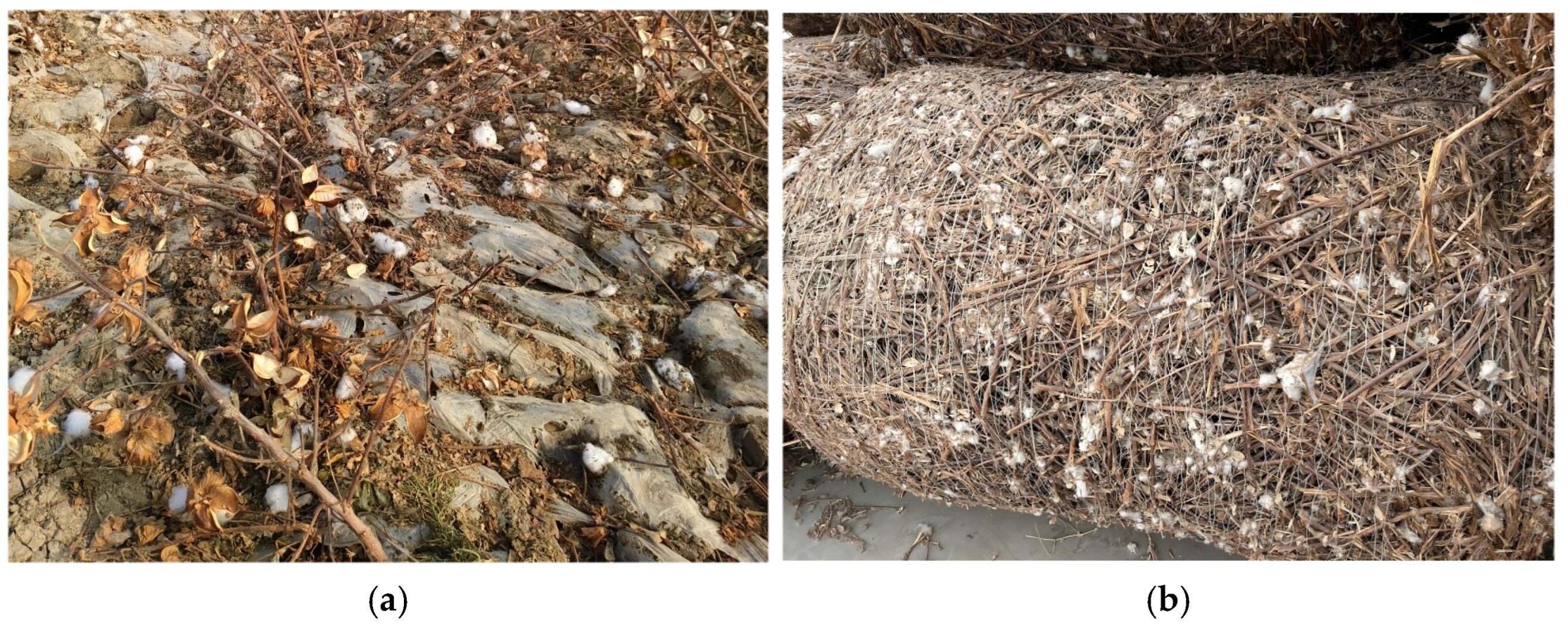
The cotton stalks and cotton residues mixture used in this study was derived from the cotton cultivar Xinluzao 48. This cultivar is grown in Aksu Prefecture, Xinjiang Uyghur Autonomous Region. Cotton harvesting was completed first. Livestock then grazed on the side branches and bolls of the cotton stalks. Samples were collected in November 2025, from cotton fields in Shaya County, Aksu Prefecture. A cotton stalk harvesting and baling machine was used for sampling, as shown in Figure 1.

In this study, cotton residues are defined as fibrous by-products retained in mechanically harvested cotton stalks. They are mainly composed of unginned cotton fiber agglomerates that were not collected during mechanical harvesting, with a small amount of broken boll shells and fine leaf debris attached to fiber surfaces. Woody short branches, weeds, and soil particles were manually removed during sample preparation to ensure material homogeneity.

2.2. Intrinsic Parameter Determination

2.2.1. Particle Size Distribution of Materials

The mechanically harvested cotton stalks and cotton residues mixture was unpacked first. A 4 kg sample was randomly collected using the quartering method [28]. Each sampling was repeated three times. Samples were sealed in plastic bags with plastic wrap.

Manual sorting was conducted based on both morphological and dimensional criteria:

• Materials with an obvious lignified stalk structure and length > 100 mm were classified as cotton stalks.
• Materials with fibrous agglomerate morphology and particle size in the range of 25–65 mm, dominated by cotton fibers, were classified as cotton residues. Fiber clusters attached to cotton stalk surfaces were stripped off and included in the cotton residue fraction.

After sorting, the length and mass of cotton stalks were measured with a tape measure and electronic balance. The size and mass of cotton residues were measured with a vernier caliper and electronic balance. The mass proportions of cotton stalks and cotton residues were 97.81% and 2.19%, respectively. The particle size distribution and mass proportions of cotton stalks and cotton residues are shown in

Table 1. Particle size distribution and mass proportion of cotton stalks and cotton residues.

Sample	Particle Size Distribution						Total Mass Proportion (%)
Cotton Stalks	Particle Size Interval (mm)	(100, 200]	(200, 300]	(300, 400]	(400, 500]	[500, 600)	97.81
	Mass Proportion (%)	14.17	26.42	26.17	16.84	16.40
Cotton Residues	Particle Size Interval (mm)	(25, 35]	(35, 45]	(45, 55]	(55, 65]	(65, ∞)	2.19
	Mass Proportion (%)	7.24	17.84	21.57	53.35	0

.

2.2.2. Moisture Content and Density Determination of Materials

Cotton residue samples (2 g each) were selected and chopped. The moisture content was measured using a DHS-20A electronic moisture analyzer (accuracy: 0.001 g; Supplier: Shanghai Yixin Scientific Instrument Co., Ltd., Shanghai, China). Each test was repeated three times, and the average value was taken. Cotton residues are porous geometries formed by intertwined fibers. Direct volume measurement using water displacement or 3D scanning is not feasible. Some collected cotton residues have a regular spherical shape. Single spherical cotton residues were selected for density measurement in this study. The diameter of cotton residues was measured with a vernier caliper to calculate volume. The mass of each sample was measured with an electronic balance. Density was calculated accordingly. Five replicate tests were conducted, and the average value was taken. The moisture content and density of cotton residues were 5.92% and 85.43 kg·m⁻³, respectively.

It should be noted that the density obtained here is the apparent density of individual cotton residue agglomerates (including internal pores between fibers), not the true density of pure cotton cellulose. This value corresponds to the particle density parameter in the DEM model, where each DEM particle represents one intact cotton residue agglomerate.

2.2.3. Determination of Elastic Modulus and Poisson’s Ratio of Materials

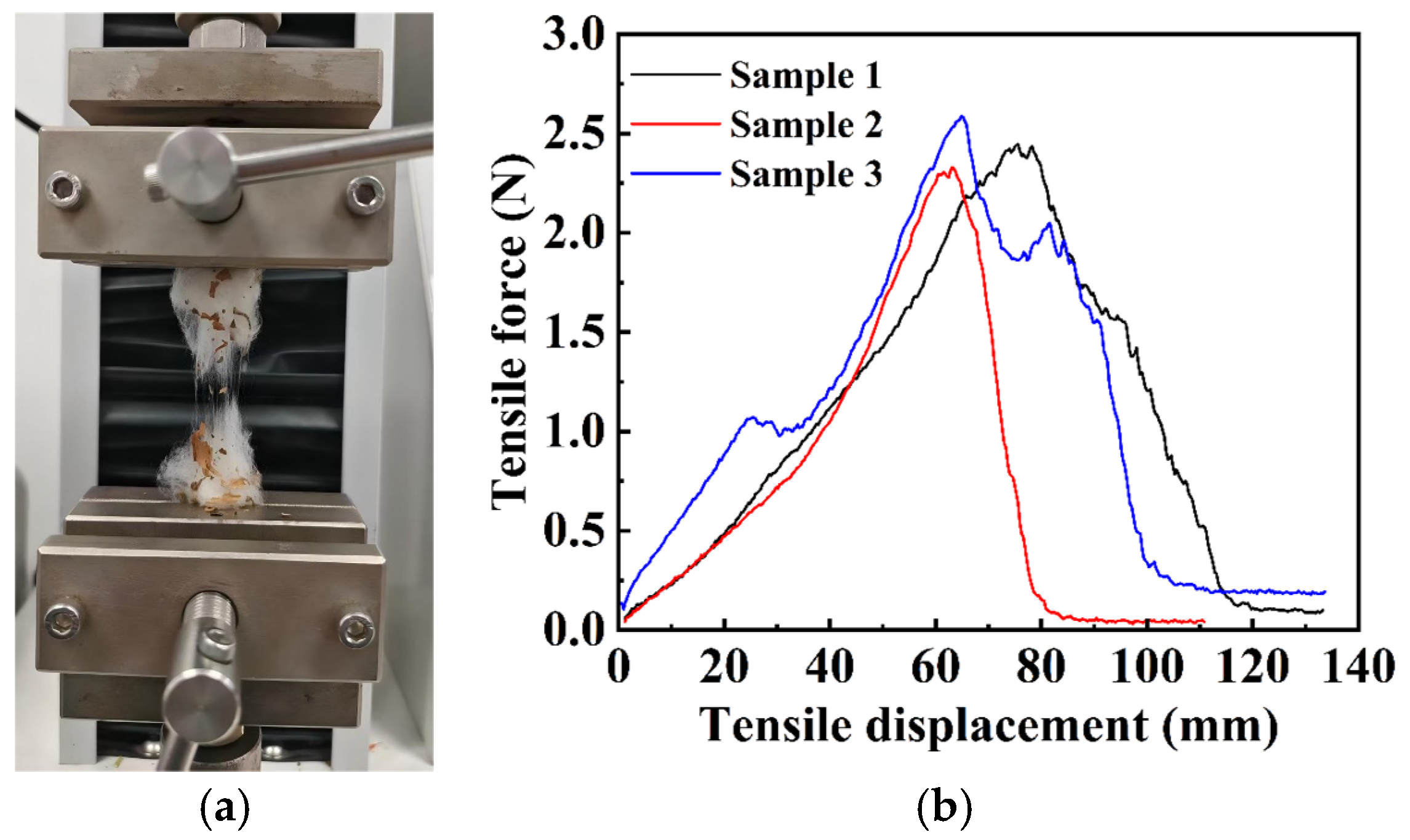
The tensile test is a common method for measuring the elastic modulus and Poisson’s ratio of materials [29,30]. In this study, an XK-207s universal testing machine (range: 100 kg; Supplier: Dongguan Xinke Instrumentation Co., Ltd., Dongguan, China) was used to measure and calculate the apparent equivalent elastic modulus and Poisson’s ratio of cotton residues. Large intact cotton residue agglomerates were selected and manually cut and kneaded into cylindrical specimens with a total length of 60 mm and a diameter of 30 mm, without additional compaction. The gauge length (the free deformation section between the upper and lower fixtures) was set to 40 mm, with 10 mm of each end of the specimen clamped by the fixture. During the test, tensile loading was performed at a constant speed of 2 mm/s. The test was paused after 15 s of loading, which falls within the approximately linear ascending section of the force-displacement curve. The axial elongation and radial diameter change in the specimen were measured at this state, as shown in Figure 2.

The apparent equivalent elastic modulus and apparent Poisson’s ratio were calculated based on the measured deformation and the initial gauge dimensions of the specimen. Since cotton residue is a porous fiber agglomerate without a strict intrinsic linear elastic stage, the parameters obtained by this method characterize the macroscopic equivalent stiffness and deformation characteristics of the agglomerate in the apparent linear deformation stage. They serve as equivalent input parameters for DEM simulation, rather than the intrinsic mechanical parameters of pure cellulose material.

Each group of tests was repeated 3 times, and the average value and sample standard deviation were adopted as the final results. The apparent equivalent elastic modulus of cotton residues is 9.79 kPa with a standard deviation of 0.42 kPa, and the apparent Poisson’s ratio is 0.36 with a standard deviation of 0.029.

The shear modulus G is related to the elastic modulus E and Poisson’s ratio $\upsilon$ by Equation (1). The shear modulus of cotton residues was calculated using this relationship. Based on previous studies [31], the intrinsic parameters of cotton stalks, cotton residues and steel are summarized in

Table 2. Apparent equivalent DEM parameters of materials and steel.

Sample	Elastic Modulus (GPa)	Poisson’s Ratio	Shear Modulus (GPa)	Density (kg·m−3)
Cotton Stalks	1.86	0.35	0.69	1020
Cotton Residues	9.79 × 10−6	0.36	3.59 × 10−6	85.43
Steel	206.44	0.3	79.4	7850

.

$$G={\displaystyle \frac{E}{2(1+\upsilon )}}$$

(1)

where G is the shear modulus, in GPa. E is the elastic modulus, in GPa. $\upsilon$ is Poisson’s ratio.

2.3. Discrete Element Model Construction

2.3.1. Discrete Element Model Development

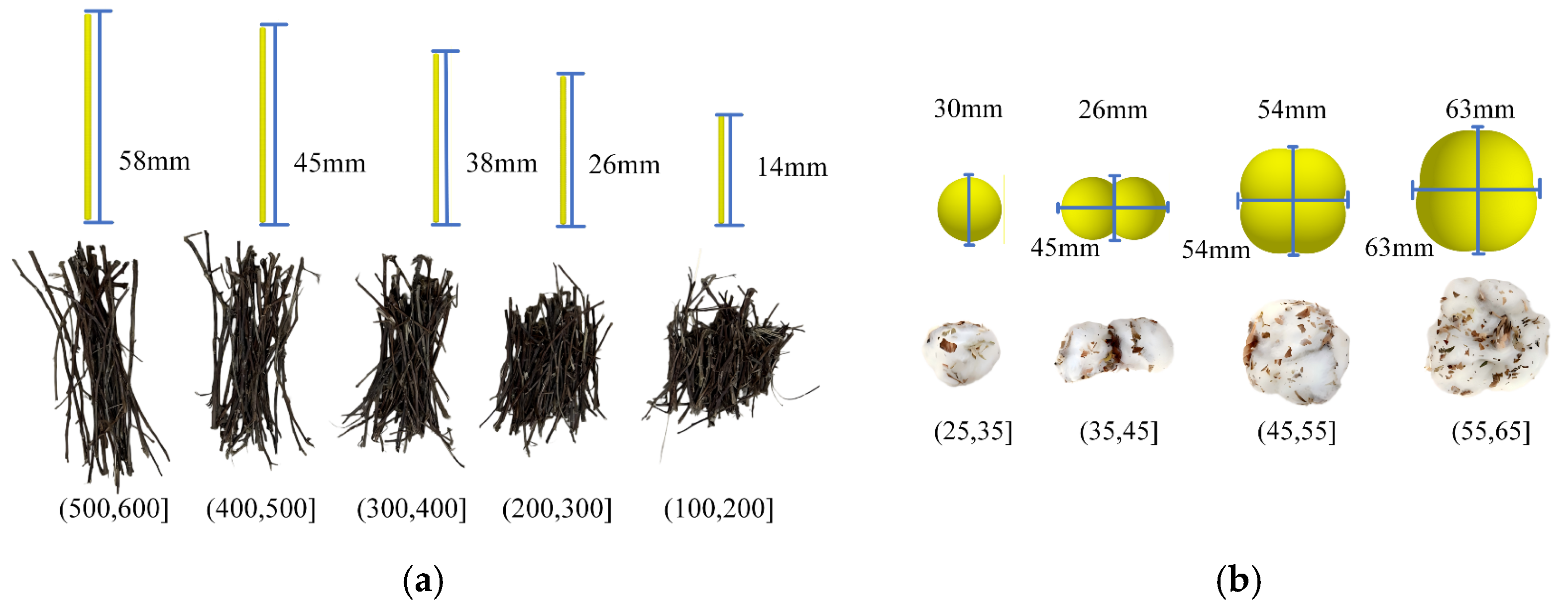
Based on the measurement results in Table 1 and the geometric morphology of cotton stalks and cotton residues, five cotton stalk models and four cotton residue models were developed. Following a standard modeling approach for cotton stalks [31], the cotton stalk models were filled with spherical particles 10 mm in diameter. Cotton residues were divided into four typical particle types according to actual measurements. Each type was filled with spherical particles of 30, 26, 40, and 50 mm in diameter, respectively. The final discrete element models of cotton stalks and cotton residues are presented in Figure 3.

An equivalent agglomerate modeling strategy was adopted for cotton residues in this work. Instead of modeling individual cotton fibers at the microscale, each DEM particle represents a macroscopic cotton residue agglomerate, which is consistent with the particle size distribution measured in physical tests. Accordingly, all contact parameters calibrated in this study (coefficient of restitution, friction coefficients, and JKR surface energy) are macroscopic equivalent parameters at the agglomerate scale. Specifically, the JKR surface energy characterizes the comprehensive adhesion effect between cotton residue agglomerates, including van der Waals forces between surface fibers and mechanical entanglement of fiber filaments, rather than the molecular-level surface energy of pure cellulose. This approach balances computational efficiency and physical fidelity, and is a widely accepted treatment for DEM simulation of fibrous agricultural materials.

2.3.2. Contact Models

The Hertz–Mindlin no slip contact model only considers the elastic deformation of materials. It does not account for the cohesive forces between particles. The Hertz–Mindlin with JKR model incorporates adhesion into the particle contact model based on Hertz–Mindlin theory. It better describes the viscoelastic properties of particles and accounts for the effect of cohesive forces on particle motion. Both cotton stalks and cotton residues in the mixture are discrete materials. No adhesion or agglomeration occurs between cotton stalks–cotton stalks, cotton residues–cotton stalks, cotton stalks–steel, or cotton residues–steel. However, strong adhesion and agglomeration exist between cotton residues–cotton residues. Therefore, the Hertz–Mindlin no slip contact model was selected to analyze the contact characteristics of these four material pairs. The Hertz–Mindlin with JKR model was used to analyze the contact characteristics between cotton residues–cotton residues. The coefficient of restitution, rolling friction coefficient, static friction coefficient, and surface energy for this pair were determined through angle of repose simulation tests.

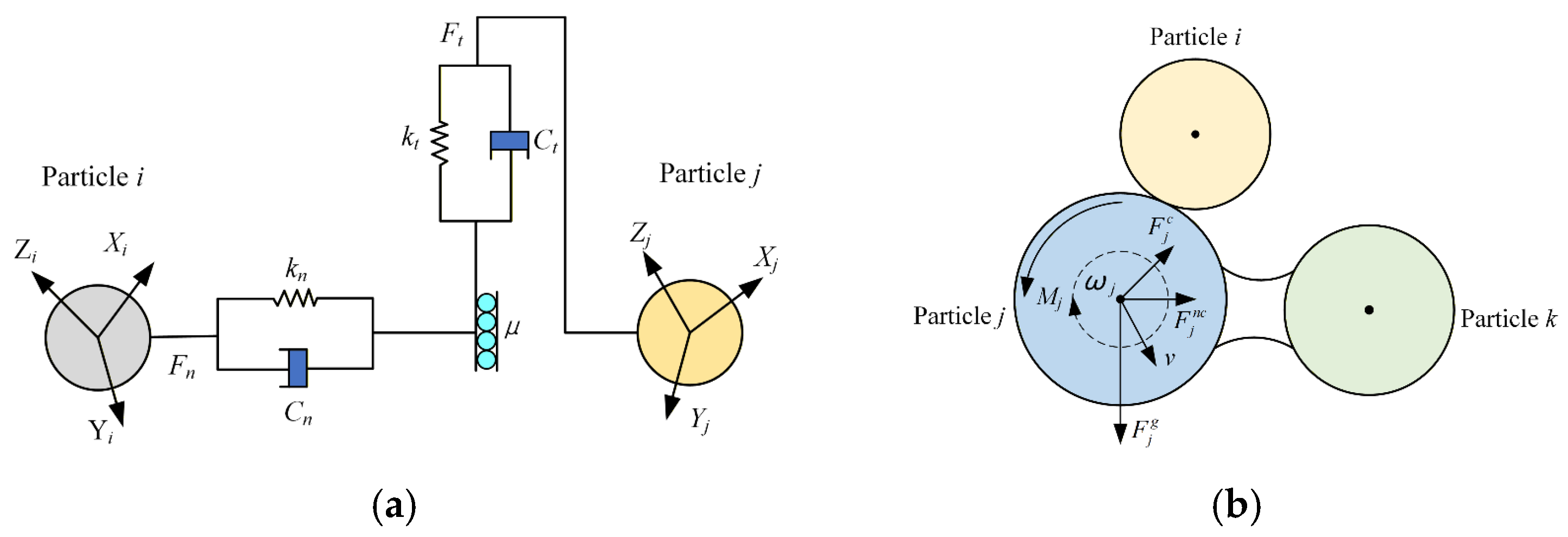
The Hertz–Mindlin no slip contact model calculates normal forces based on Hertz contact theory. Its tangential forces are derived from Mindlin’s tangential contact method [32,33]. Damping components are introduced for both normal and tangential forces. Tangential forces follow Coulomb’s friction law. Rolling friction is modeled as a directional constant torque. A schematic of this contact model is shown in Figure 4a. This study involves extensive mixing of different materials. Materials exhibit complex motion patterns inside the equipment. Numerous contact collisions occur between particles and between particles and equipment. Calculating these collision forces is complex and computationally intensive. The discrete element method obtains particle motion by solving Newton’s equations of motion. These equations are presented as Equations (2) and (3). Particle velocities and positions are numerically integrated at each time step. This integration updates the velocity and position of each particle. The particle calculation model is shown in Figure 4b.

$$I_j{\displaystyle \frac{d{\omega }_j}{dt}}=M_j$$

(2)

where I_j is the moment of inertia, in kg·m². ω_j is the angular velocity of particle j, in rad/s. M_j is the contact torque acting on particle j, in N·m. t is time, in s.

$$m_j{\displaystyle \frac{d{v}_j}{dt}}=F_j^g+F_j^c+F_j^{nc}$$

(3)

where v_j is the translational velocity of the particle, in m/s. m_j is the mass of the particle, in kg. $F_j^g$ is the gravitational force acting on particle j, in N. $F_j^c$ is the contact force between particle j and other particles, in N. $F_j^{nc}$ is the contact force between particle j and the equipment, in N.

The Hertz–Mindlin with JKR cohesive model introduces van der Waals adhesive forces at contact interfaces. It is built upon the fundamental principles of Hertz–Mindlin theory. JKR theory modifies the normal contact force equation. It adds an attractive term related to the surface energy of contact materials, as shown in Equation (4):

$$F_{\mathrm{n}}={\displaystyle \frac{4}{3}}E*\sqrt{R*}{\delta }_{\mathrm{n}}^{3/2}-\sqrt{4\pi \gamma E*R*{\delta }_{\mathrm{n}}^{3/2}}$$

(4)

where F_n is the normal contact force between particles, in N. E* is the equivalent Young’s modulus, in Pa. R* is the equivalent radius, in m. δ_n is the normal overlap, in m. γ is the surface energy, in J/m².

This equation demonstrates that the JKR model predicts a finite contact area between particles. This contact area exists even when the normal external load is zero, rather than complete separation. Therefore, to separate two adhesive particles, a sufficiently large reverse tensile force must be applied. This force is required to overcome the surface adhesion energy. The critical pull-off force needed to completely separate two adhesive particles is expressed by Equation (5):

$$F_{pull\text{-}off}={\displaystyle \frac{3}{2}}\pi \gamma R^{*}$$

(5)

where F_pull-off is the minimum normal tensile force to separate two adhesive particles, in N. R* is the equivalent radius, in m. γ is the surface energy, in J/m².

Cotton residues consist of fine, soft fibers with an extremely high specific surface area. This results in significant van der Waals forces between individual fibers. These forces cause strong agglomeration and cohesion phenomena. These phenomena cannot be accurately characterized by friction coefficients alone. The Hertz–Mindlin with JKR cohesive model explicitly accounts for this adhesion through the surface energy parameter. It is therefore a viable choice for simulating the contact characteristics of cotton residues. This study will use this model to conduct angle of repose simulation tests for cotton residues. The contact parameters between cotton residues and cotton residues will be calibrated by comparing simulation results with experimental measurements. Considering the low apparent equivalent elastic modulus of cotton residue materials, the Rayleigh time step of the simulation system was calculated based on the minimum particle size and material mechanical parameters. The simulation time step was set to 20% of the Rayleigh time step to ensure the numerical stability of the discrete element calculation. Under this time step setting, the maximum overlap between particles is less than 0.5% of the particle radius, which is within the generally accepted range for DEM simulations. The small particle overlap has no significant effect on the simulation results of material flow, conveying, and vibratory layering behavior.

2.4. Calibration of Contact Parameters Between Materials

Previous studies have shown [31] that the coefficient of restitution for cotton stalks–cotton stalks is 0.5. The corresponding static friction coefficient is 0.41, and the rolling friction coefficient is 0.06. For cotton stalks–steel, the coefficient of restitution is 0.5. Its static friction coefficient is 0.37, and the rolling friction coefficient is 0.08.

2.4.1. Determination of Inter-Particle Collision Coefficient of Restitution

The coefficient of restitution between materials is defined as the ratio of the normal separation velocity after collision to the relative approach velocity before collision. It accurately reflects the ability of an object to recover its original shape after impact [34,35]. In this study, the coefficient of restitution between different material pairs was measured using the free-fall test method [25].

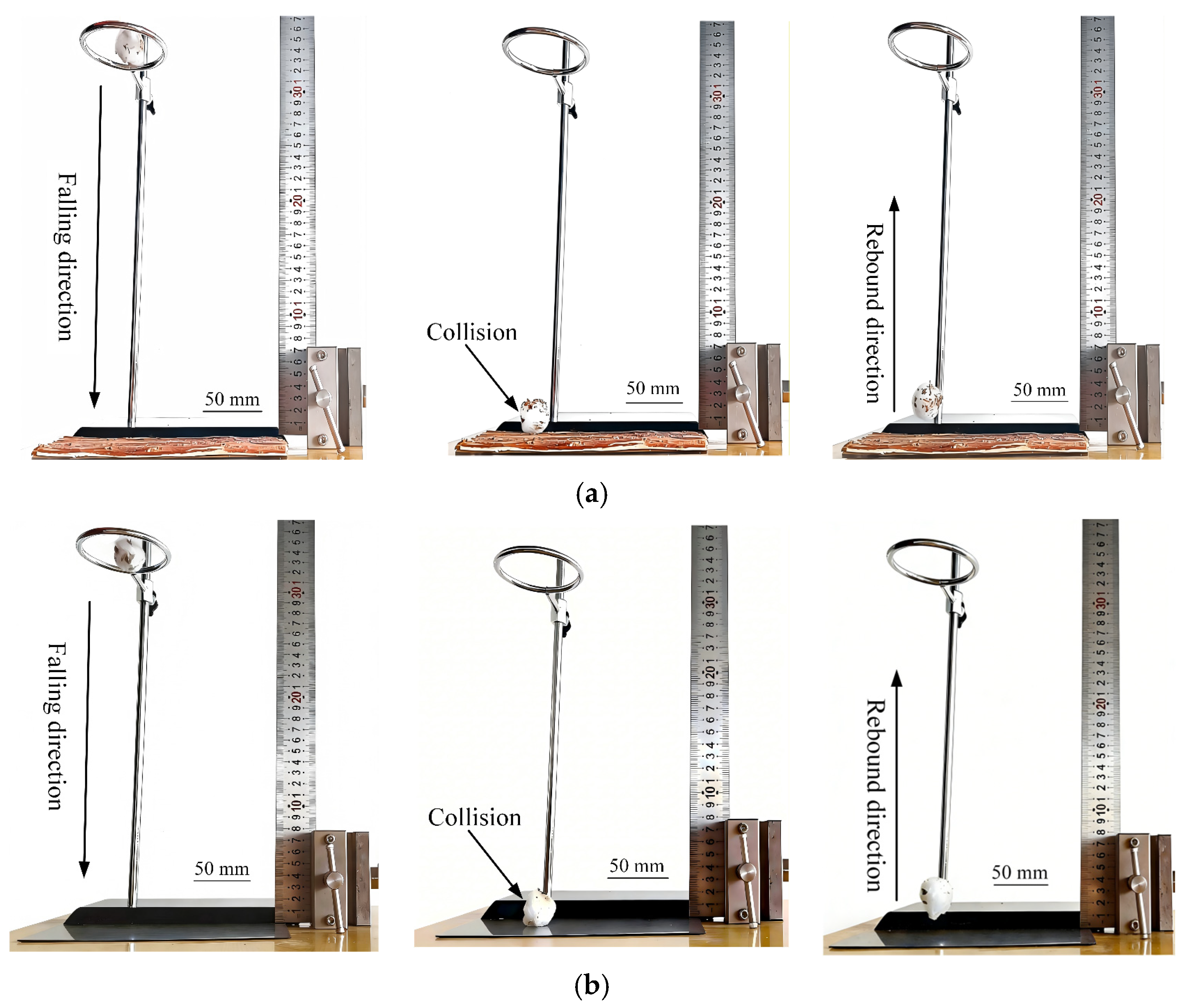
A DCXG13-30 high-speed camera (frame rate: 400 fps; Supplier: Shenzhen Jierui Weitong Electronic Technology Co., Ltd., Shenzhen, China) was used to record the collision process of the materials. Steel and cotton stalk plates were fabricated as impact plates. Each plate measured 200 mm in length and 100 mm in width. The steel plate was 2 mm thick, and the cotton stalks plate was 5 mm thick. Cotton stalk specimens (30 mm in length and 10 mm in diameter) were selected. Single spherical cotton residues specimens with a diameter of 30 mm were also used as impact samples. During the coefficient of restitution measurement, each specimen was dropped freely from the center of a steel ring at a height of 300 mm. It collided with the material affixed to the impact plate upon reaching the plate surface. After rebounding, the specimen underwent vertical projectile motion. The maximum rebound height (h_i) of the specimen after collision was captured. The coefficient of restitution between materials was calculated using Equation (6). Each test was repeated 10 times. The parameter range and average value of hi for the coefficients of restitution were determined. The experimental process is illustrated in Figure 5.

$$e_{\mathrm{i}}=\sqrt{{\displaystyle \frac{h_{\mathrm{i}}}{H_0}}}$$

(6)

where e_i is the coefficient of restitution between materials. H₀ is the initial height of the specimen, in mm. h_i is the maximum rebound height of the specimen after collision, in mm.

Based on Equation (6), the coefficient of restitution e ranges from 0.294 to 0.334 for cotton stalks–cotton residues. It ranges from 0.273 to 0.369 for cotton residues–steel.

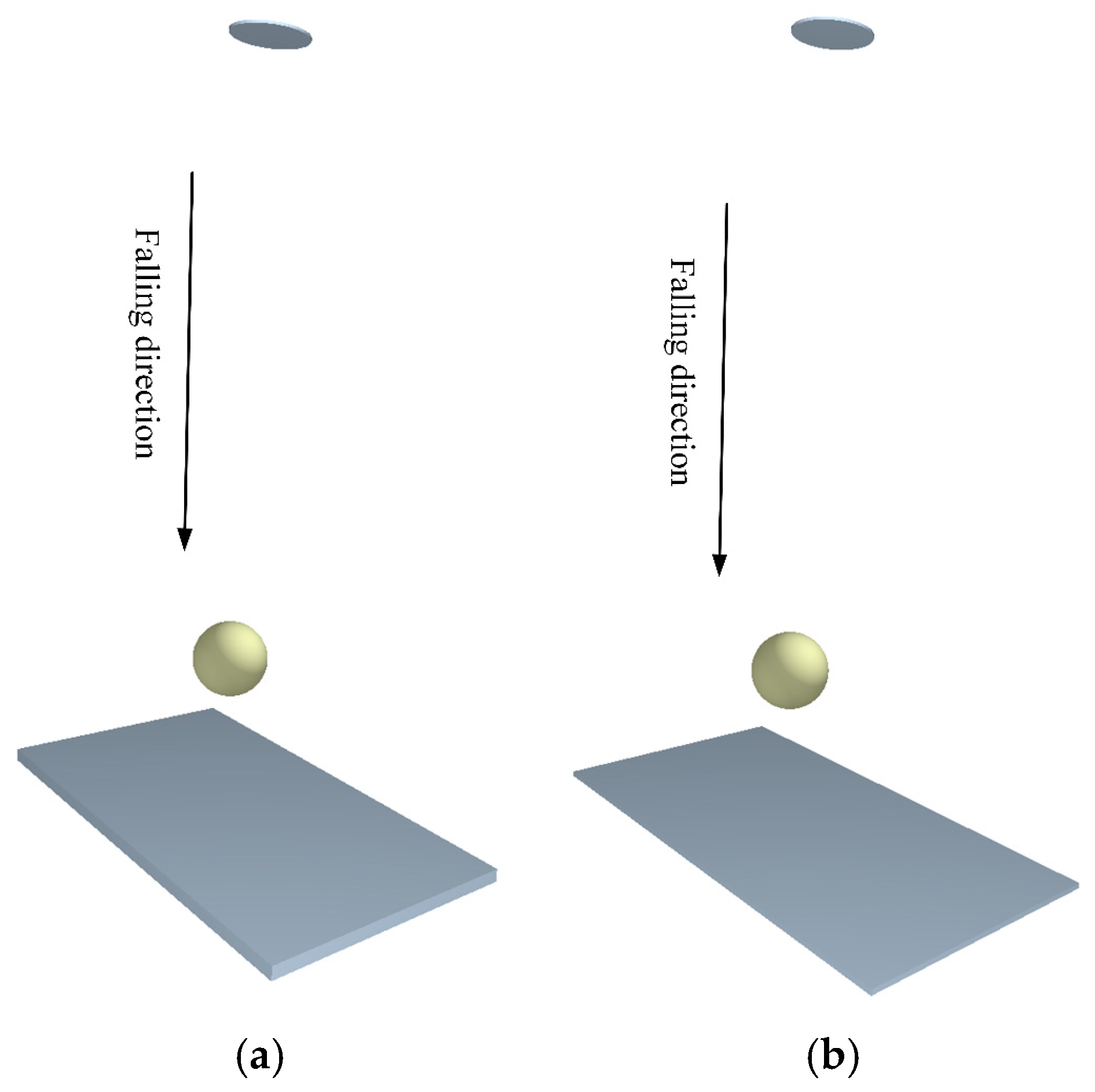
The coefficient of restitution is affected by more than just the intrinsic parameters of materials. It also depends on particle geometry and size, impact material type, and impact material thickness. Therefore, to ensure simulation accuracy, impact plate models were established with the same geometry and thickness as those used in physical tests. Discrete element models were also built according to the physical test dimensions. These included 30 mm long, 10 mm diameter cotton stalks, and 30 mm diameter single spherical cotton residues. In the simulation tests, only gravity acts on the impact specimens. The static and rolling friction coefficients between specimens and impact plates have negligible effects on the maximum rebound height. Therefore, all contact parameters except the coefficient of restitution were set to 0 in the simulations. Each specimen was dropped freely from a height of 300 mm during the tests. The simulation process is illustrated in Figure 6.

Based on the coefficient of restitution ranges determined from physical tests, 10 groups of simulation tests were conducted with appropriate step sizes. Each test was repeated 10 times and the average value was calculated. The simulation test schemes and results are presented in

Table 3. Simulation test plan and results of coefficient of restitution.

Test Group No.	e	h1 (mm)	e	h2 (mm)
1	0.25	30.11	0.27	22.50
2	0.26	31.83	0.28	23.26
3	0.27	33.22	0.29	24.03
4	0.28	34.68	0.30	25.04
5	0.29	36.34	0.31	26.20
6	0.30	37.90	0.32	27.17
7	0.31	39.30	0.33	28.17
8	0.32	41.07	0.34	29.30
9	0.33	42.84	0.35	30.44
10	0.34	43.03	0.36	32.07

. The average maximum rebound heights h after collision are 26.3 mm for cotton stalks–cotton residues and 32.5 mm for cotton residues–steel, respectively.

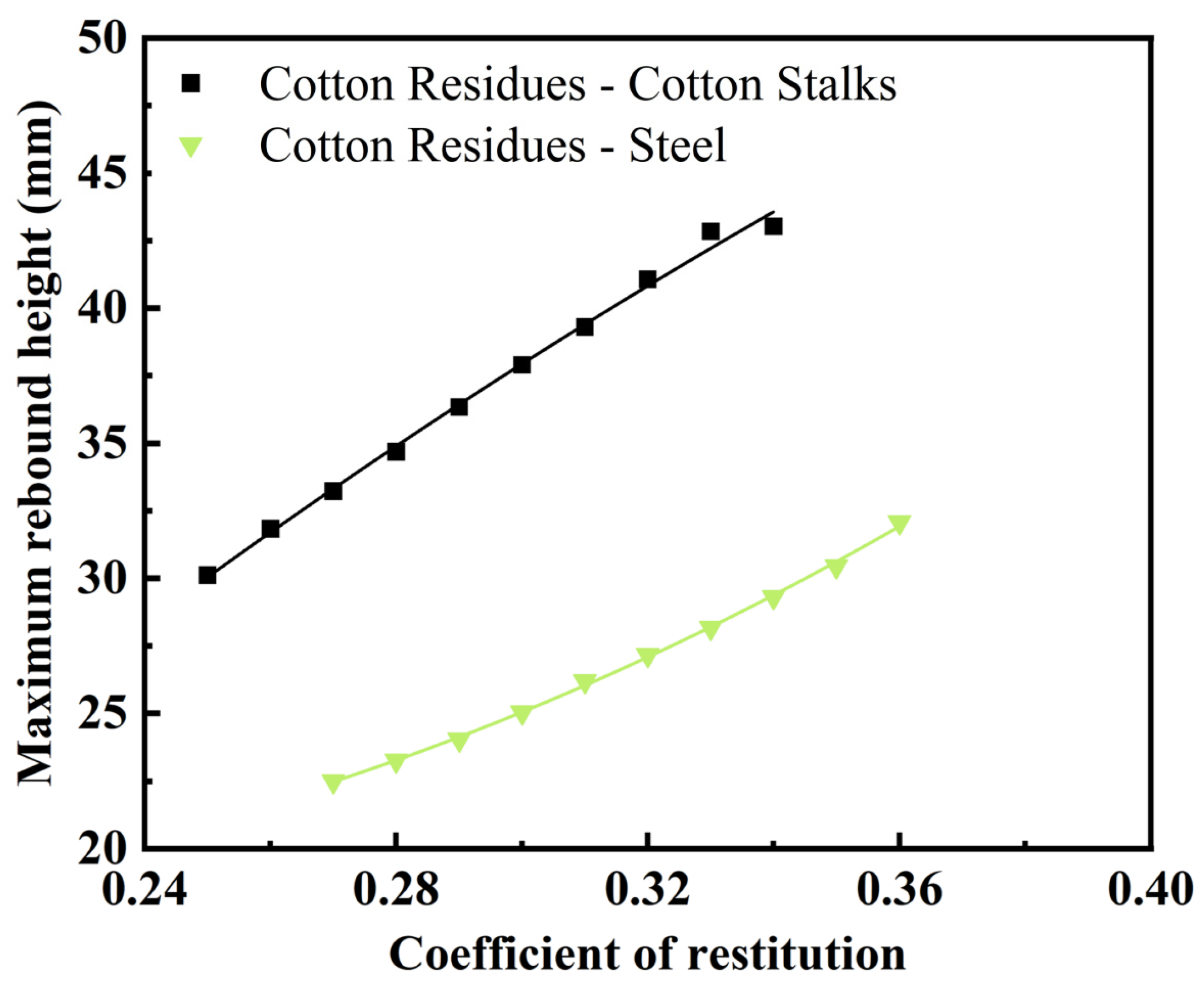
Quadratic polynomial fitting was performed on the maximum rebound height and coefficient of restitution from the test results. The correlation between the coefficient of restitution e and maximum rebound height (h) for different material pairs was obtained. The fitting curves are shown in Figure 7. The quadratic fitting equations for cotton stalks–cotton residues and cotton residues–steel are presented as Equations (7) and (8):

$$h_1=-189.773e^2+262.281e-23.669(R^2=0.9956)$$

(7)

$$h_2=317.424e^2-95.068e+25.006(R^2=0.999)$$

(8)

where e is the coefficient of restitution between materials. h₁ is the maximum rebound height of the specimen after collision between cotton stalks and cotton residues, in mm. h₂ is the maximum rebound height of the specimen after collision between cotton residues and steel, in mm.

The maximum rebound heights measured in physical tests were substituted into Equations (7) and (8). The coefficients of restitution were calculated as 0.228 for cotton stalks–cotton residues and 0.364 for cotton residues–steel. The corresponding coefficients of restitution were set in EDEM 2022 software. The simulated maximum rebound heights were 26.89 mm and 32.97 mm, respectively. The relative errors compared with the measured values were 2.24% and 1.45%, respectively. These results indicate that the calibrated simulation results are consistent with physical tests. Therefore, the coefficients of restitution for EDEM simulations were determined as 0.228 and 0.364 for the two material pairs.

2.4.2. Determination of Static Friction Coefficients Between Materials

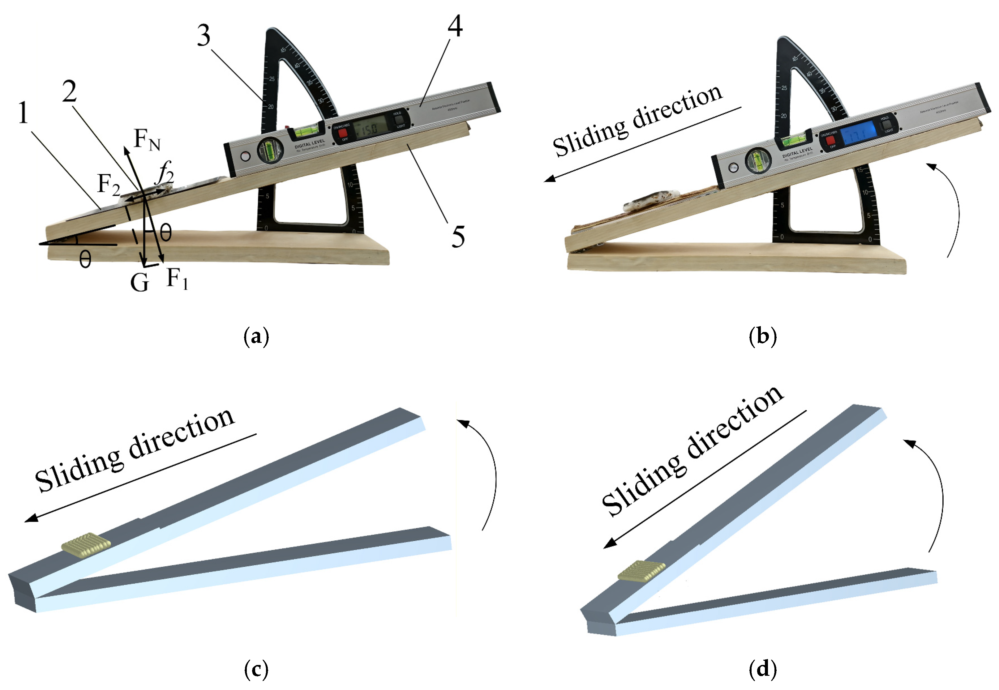
The inclined plane method was used to measure friction coefficients between materials in this study [36,37]. A self-made inclinometer was employed to measure static friction coefficients for cotton stalks–cotton residues and cotton residues–steel, as shown in Figure 8. Before the tests, friction surfaces were prepared for different materials. Cotton stalks and steel surfaces measured 200 mm in length and 100 mm in width. Cotton residues surfaces measured 100 mm in length and 50 mm in width. During the test, the prepared cotton stalks or steel friction surface were fixed on the inclined plane. A calibrated angle measuring instrument was also fixed on the plane. A cotton residue specimen was placed stably on the upper part of the inclined plane. The inclined plane was raised slowly. The plane was locked and the inclination angle was recorded when the specimen started to slide. The static friction coefficient between materials was calculated using Equation (9). Each test was repeated 10 times. The average value of the inclination angle(θ) was calculated. The static friction coefficient (μ) ranges were 0.589–0.661 for cotton stalks–cotton residues and 0.249–0.303 for cotton residues–steel.

$$\mu ={\displaystyle \frac{G\sin \theta }{G\cos \theta }}=\tan \theta$$

(9)

where μ is the static friction coefficient between materials. G is the gravitational force acting on the specimen, in N. θ is the inclination angle of the inclined plane, in °.

Based on the physical test results, 10 groups of simulation tests for static friction coefficients were conducted with appropriate step sizes. The test design schemes and results are presented in

Table 4. Simulation test plan and results for the static coefficient of friction.

Test Group No.	μ	θ1 (°)	μ	θ2 (°)
1	0.58	29.26	0.23	13.43
2	0.59	30.23	0.24	14.16
3	0.60	31.34	0.25	14.87
4	0.61	31.85	0.26	15.38
5	0.62	32.25	0.27	15.91
6	0.63	32.57	0.28	16.35
7	0.64	32.98	0.29	16.65
8	0.65	33.28	0.30	16.87
9	0.66	33.87	0.31	17.59
10	0.67	34.25	0.32	17.87

. To reduce the error between simulation and physical tests, 3D models of friction surfaces were established before simulations. These models were built according to the geometry of friction surfaces fabricated in physical tests. The physical models were imported into EDEM software before simulation. An automatic filling method was used to fill the cotton residues friction surface geometry with particles. The smoothing value was set to 5. The filled cotton residues particles were most similar to physical tests when the particle distribution numbers in x, y, and z directions were 30, 30, and 30, respectively. The time step was set to 0.3%. To ensure the accuracy of simulation calculations, the calibrated coefficients of restitution between materials were set before running the simulations.

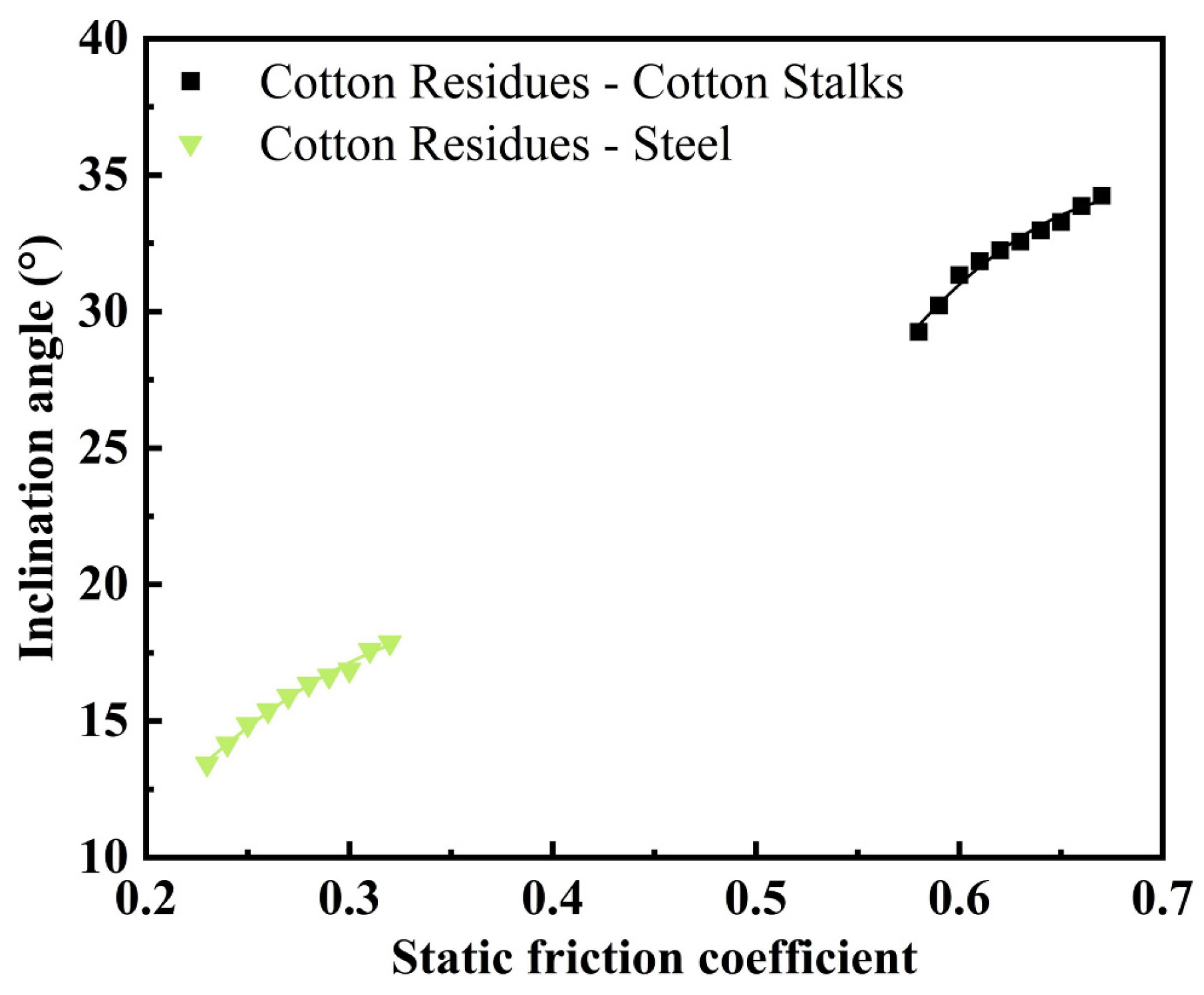
Quadratic polynomial fitting was performed on the static friction coefficient and inclined plane angle (θ) from the test results. The functional relationship between the static friction coefficient and plane angle for different material pairs was obtained. The fitting curves are shown in Figure 9. The quadratic fitting equations for cotton stalks–cotton residues and cotton residues–steel are presented as Equations (10) and (11):

$${\theta }_1=-345.83{\mu }^2+483.08\mu -134.36(R^2=0.983)$$

(10)

$${\theta }_2=-210.98{\mu }^2+163.45\mu -12.91(R^2=0.9933)$$

(11)

where μ is the static friction coefficient between materials. θ₁ is the inclination angle of the inclined plane when measuring the static friction coefficient for cotton stalks–cotton residues, in °. θ₂ is the inclination angle of the inclined plane when measuring the static friction coefficient for cotton residues–steel, in °.

The average inclination angles (θ) measured in physical tests were 32.81° and 15.64°. These values were substituted into Equations (10) and (11), respectively. The static friction coefficients were calculated as 0.632 for cotton stalks–cotton residues and 0.266 for cotton residues–steel. The corresponding static friction coefficients were set in EDEM software. The simulated inclination angles (θ) were 32.15° and 15.48°, respectively. The relative errors compared with the measured values were 2.01% and 1.02%, respectively. These results indicate that the calibrated simulation results are consistent with physical tests. Therefore, the static friction coefficients for EDEM simulations were determined as 0.632 and 0.266 for the two material pairs.

2.4.3. Determination of Rolling Friction Coefficients Between Materials

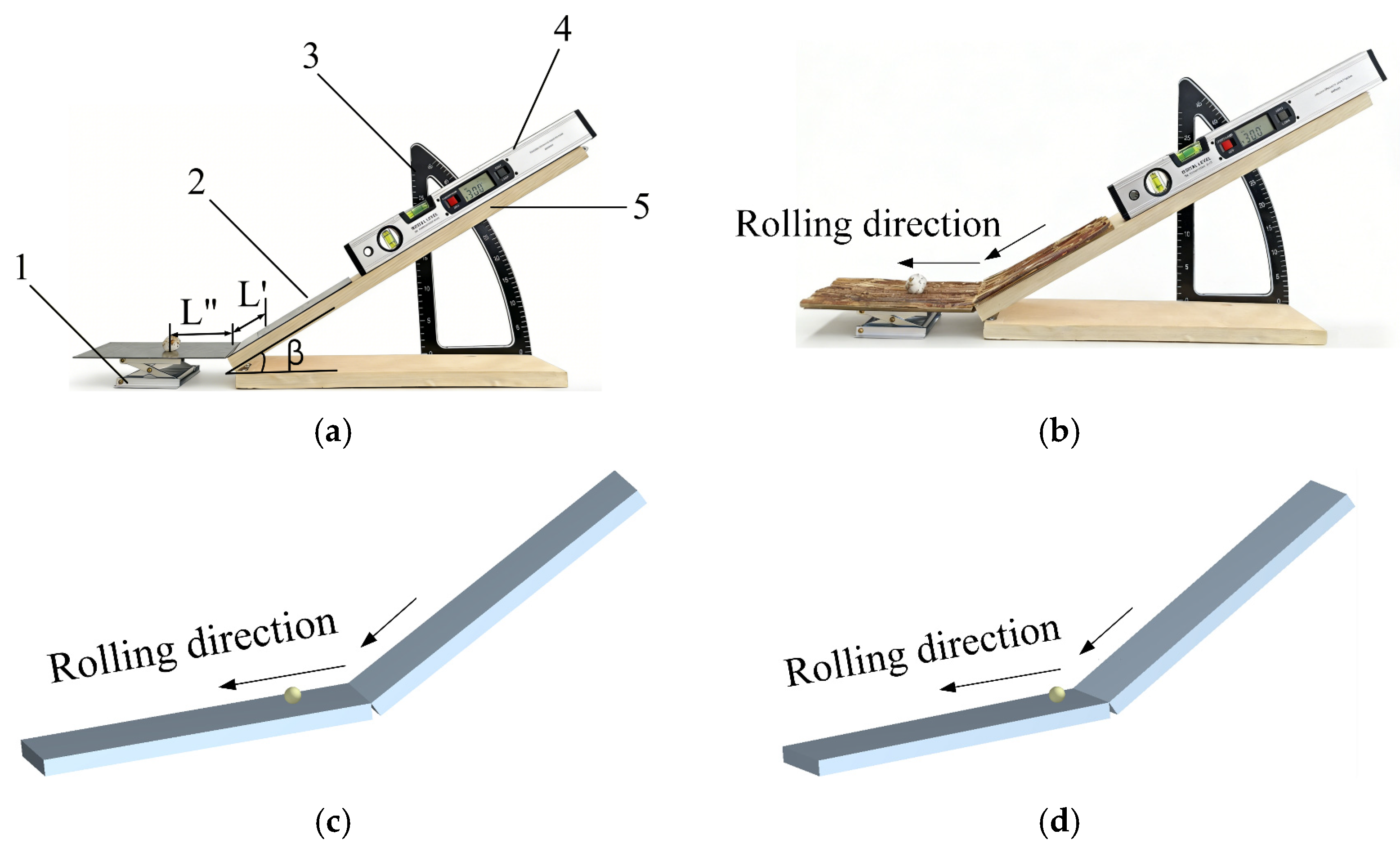
The rolling friction coefficient can be calculated using the law of conservation of energy. A self-made rolling friction coefficient test bench was used in this study. It was employed to measure the rolling friction coefficients for cotton stalks–cotton residues and cotton residues–steel, as shown in Figure 10. Before the tests, two friction surfaces were fabricated for cotton stalks and steel. Each measured 200 mm in length and 100 mm in width. Single spherical cotton residues particles with a diameter of 30 mm were selected. Cylindrical cotton stalk specimens (30 mm in length and 10 mm in diameter) were also prepared. During the test, one friction surface was fixed at an incline on the upper part of the bench. The other friction surface was placed horizontally at the lower end of the inclined surface. A spherical cotton residues specimen was released from the 30 mm position on the inclined surface. The rolling distance of the specimen on the horizontal friction surface was recorded. The rolling friction coefficient between materials was calculated using Equation (12). Each test was repeated 10 times. The average rolling distance of the specimens was calculated. The rolling friction coefficient (μ_r) ranges were 0.193–0.213 for cotton stalks–cotton residues and 0.153–0.172 for cotton residues–steel.

$${\mu }_{\mathrm{r}}={\displaystyle \frac{{GL}^{\prime }\sin \beta }{G(L^{\prime }\cos \beta +L^{″})}}={\displaystyle \frac{L^{\prime }\sin \beta }{L^{\prime }\cos \beta +L^{″}}}$$

(12)

where μ_r is the rolling friction coefficient between materials. G is the gravitational force acting on the specimen, in N. $L^{\prime }$ is the rolling distance of the specimen on the inclined plane, in mm. $L^{″}$ is the rolling distance of the specimen on the horizontal plane, in mm. β is the inclination angle of the inclined plane, in °.

According to the rolling friction coefficient ranges obtained from physical tests, ten groups of simulation tests were carried out with proper step sizes. The test schemes and results are listed in

Table 5. Simulation test plan and results of rolling friction coefficient.

Test Group No.	μr	L1″ (mm)	μr	L2″ (mm)
1	0.191	48.30	0.150	70.37
2	0.194	46.22	0.153	68.56
3	0.197	45.95	0.156	67.13
4	0.200	45.14	0.159	64.33
5	0.203	43.65	0.162	64.95
6	0.206	42.89	0.165	60.93
7	0.209	41.47	0.168	57.28
8	0.212	40.75	0.171	55.59
9	0.215	39.65	0.174	53.85
10	0.218	36.93	0.177	51.04

. To narrow the deviation between simulation and physical tests, three-dimensional friction surface models were established. A single spherical cotton residues particle model with a diameter of 30 mm was also built. All models were consistent with the geometric features used in physical tests. The time step was set to 0.3%. To guarantee reliable simulation outcomes, the calibrated coefficient of restitution and static friction coefficient were preset in EDEM before calculation.

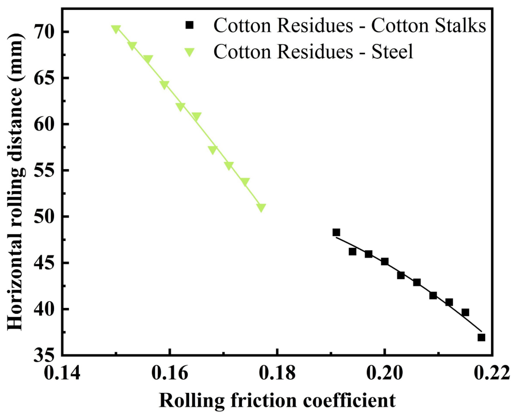
Quadratic polynomial fitting was conducted on rolling friction coefficients and horizontal rolling distances of cotton residues. The functional relationships between these two parameters for different material pairs were obtained. The fitting curves are displayed in Figure 11. The quadratic fitting equations for cotton stalks–cotton residues and cotton residues–steel are given in Equations (13) and (14).

$${L_1}^{″}=-4027.8{{\mu }_{\mathrm{r}}}^2+1271.4{\mu }_{\mathrm{r}}-48.169(R^2=0.982)$$

(13)

$${L_2}^{″}=-2436.9{{\mu }_{\mathrm{r}}}^2+76.028{\mu }_{\mathrm{r}}+114(R^2=0.995)$$

(14)

where μ_r represents the rolling friction coefficient between different materials. ${L_1}^{″}$ is the rolling distance of cotton residues specimens on horizontal cotton stalks surfaces, in mm. ${L_2}^{″}$ is the rolling distance of cotton residues specimens on horizontal steel surfaces, in mm. β denotes the inclination angle of the inclined plane, in degrees.

The average horizontal rolling distances of cotton residues obtained from physical tests were 45.48 mm and 66.75 mm. These values were substituted into Equation (13) and Equation (14), respectively. The calculated rolling friction coefficients were 0.199 for cotton stalks–cotton residues and 0.156 for cotton residues–steel. The corresponding rolling friction coefficients were set in EDEM. The simulated horizontal rolling distances were 48.05 mm and 64.05 mm. Their relative errors against measured values were 5.65% and 4.04%. The results verified that calibrated simulation data match well with physical test data. Thus, the rolling friction coefficients of 0.199 and 0.156 were confirmed for the two material pairs in EDEM simulation.

2.5. Calibration of Contact Parameters Between Cotton Residues

2.5.1. Repose Angle Test and Determination of Contact Parameter Ranges

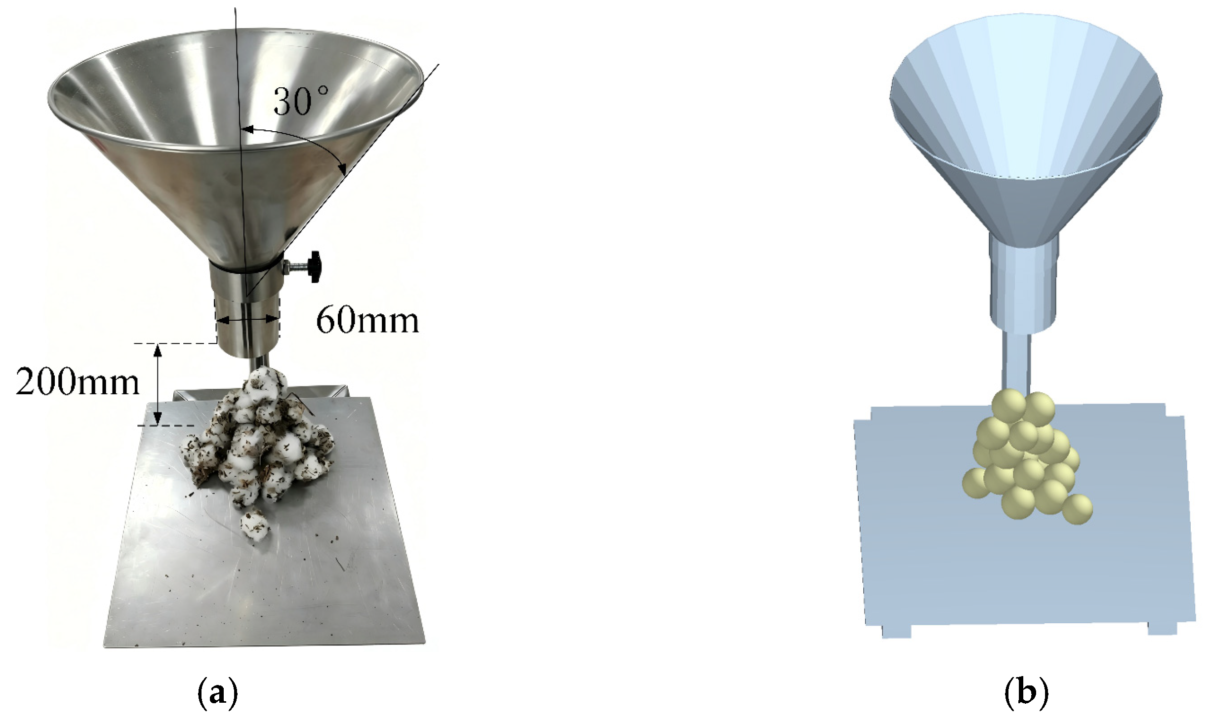
Due to the strong agglomeration and adhesion behavior of cotton residues at the macroscopic scale, the Hertz–Mindlin with JKR contact model was employed, where the surface energy parameter reflects the equivalent adhesion force between fiber agglomerates. The internal contact parameters of cotton residues cannot be directly and accurately measured by physical experiments. Therefore, the funnel method was adopted in this study to measure the angle of repose formed during the falling process of cotton residues [38,39], as shown in Figure 12. Spherical cotton residues particles were poured from the top of the funnel in the test. These particles accumulated on the stainless steel substrate and formed a conical pile. The angle of repose (Y) is mainly affected by four contact parameters. They include coefficient of restitution (X₁), rolling friction coefficient (X₂), static friction coefficient (X₃) and surface energy (X₄). Therefore, physical experiments combined with simulation tests were applied to calibrate contact parameters between cotton residues.

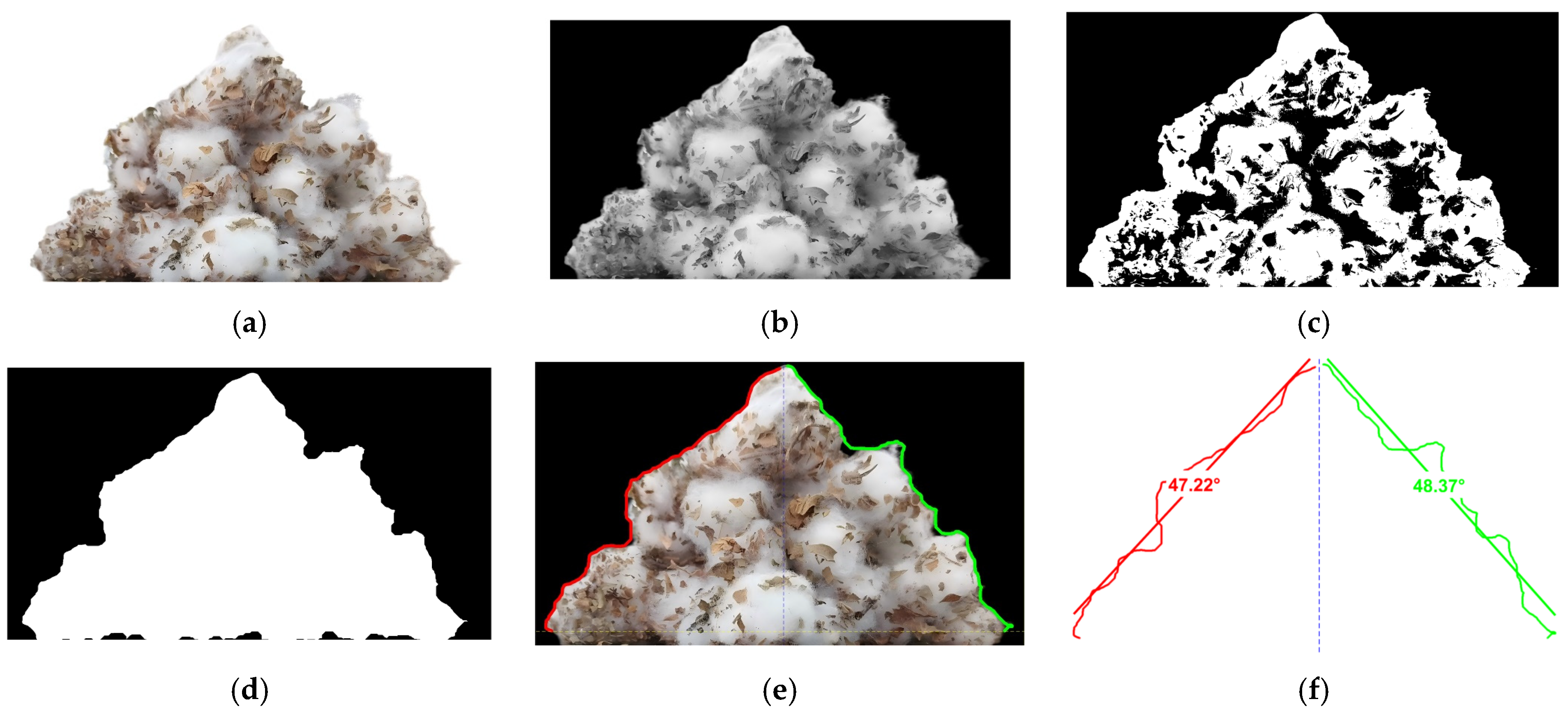
A total of 30 g of spherical cotton residues were taken from Cotton Stalks and Cotton Residues Mixture for the test. These particles were slowly poured into a funnel with a cone angle of 30° and an aperture of 60 mm. Under gravity, the materials fell onto a stainless steel substrate 200 mm below and formed a conical pile. After standing for one minute, the formed angle of repose (Y) was measured. MATLAB R2022b software was used to process pile images for high measurement accuracy. The highest point of the pile was determined and set as the central vertical line. Boundary lines on both sides of the central line were extracted and linearly fitted, as shown in Figure 13. The included angles between two fitted lines and the substrate were calculated. The average value of the two angles was defined as the tested Angle of Repose. The test was repeated five times. The final stable Angle of Repose (Y) of cotton residues was determined as 47.46°.

Cotton residues are cohesive granular materials prone to agglomeration, and their internal contact parameters cannot be accurately determined directly via physical tests. The initial parameter ranges were determined using the GEMM (Generic EDEM Material Model) database in EDEM. The GEMM tool selects feasible parameter ranges based on three input conditions: application scale, bulk density, and the experimentally measured target angle of repose. In this study, the application scale was set to “Small” to match the bench-scale test equipment, the bulk density of cotton residues was measured as 85.43 kg/m³, which falls into the category of low-density fibrous agricultural materials, and the target angle of repose was set to 47.46°, the value experimentally measured via the funnel method. Under these three constraints, the GEMM database returned multiple sets of contact parameter configurations corresponding to an angle of repose of approximately 47–48°, and the initial value ranges of contact parameters for cotton residue–cotton residue were extracted from these configurations: 0.15–0.75 for coefficient of restitution (X₁), 0.1–0.2 for rolling friction coefficient (X₂), 0.44–1.16 for static friction coefficient (X₃), and 0–14 J/m² for surface energy (X₄). These ranges are consistent with published DEM parameter values for similar fibrous agricultural materials, such as wheat straw and ramie stalk [40,41]. The surface energy range provided by the GEMM toolbox is relatively wide. Excessively high surface energy in simulations causes severe material adhesion. This phenomenon easily leads to pile collapse and brings large test errors. Friction coefficients show a positive correlation with the formation of angle of repose. The coefficient of restitution presents a negative correlation with it [42]. Single-factor optimization tests were adopted to narrow down the reasonable range of surface energy. Each group of tests was repeated ten times. The test schemes and results are shown in

Table 6. Single-factor optimization test of surface energy for cotton residues.

Test No.	Coefficient of Restitution (X1)	Rolling Friction Coefficient (X2)	Static Friction Coefficient (X3)	Surface Energy (X4)/(J/m2)	Angle of Repose (Y)/(°)
1	0.15	0.2	1.16	0	0
2	0.15	0.2	1.16	0.5	31.07
3	0.15	0.2	1.16	1	60.55
4	0.75	0.1	0.44	2	37.54
5	0.75	0.1	0.44	2.5	48.06
6	0.75	0.1	0.44	3	61.08

.

The angle of repose (Y) of cotton residues rises with the increase in static friction coefficient (X₃), rolling friction coefficient (X₂), and surface energy (X₄). It declines as the coefficient of restitution (X₁) increases. The minimum surface energy (X₄) is required to form the target angle of repose when (X₃) and (X₂) are set to maximum values and (X₁) to the minimum value. In contrast, the maximum surface energy (X₄) is needed when (X₃) and (X₂) take minimum values and (X₁) takes the maximum value. Test results show that the simulated angle of repose exceeds the measured value of 47.46° at surface energy of 1.0 J/m² and 2.5 J/m². Thus, the reasonable surface energy range is determined as 0.5–2.5 J/m². The preliminary calibrated ranges of contact parameters for cotton residues are listed in

Table 7. Value ranges of contact parameters between cotton residues.

Contact Parameter	Value
Coefficient of Restitution (X1)	0.15–0.75
Rolling Friction Coefficient (X2)	0.1–0.2
Static Friction Coefficient (X3)	0.44–1.16
Surface Energy (X4)/(J/m2)	0.5–2.5

.

2.5.2. Steepest Ascent Test and Results

To further confirm the optimal range of contact parameters between cotton residues, the steepest ascent test was carried out on the preliminarily determined parameters. These parameters included coefficient of restitution (X₁), rolling friction coefficient (X₂), static friction coefficient (X₃), and surface energy (X₄) [43,44]. The design scheme and results of the steepest ascent test are presented in

Table 8. Steepest ascent test.

Test No.	Coefficient of Restitution (X1)	Rolling Friction Coefficient (X2)	Static Friction Coefficient (X3)	Surface Energy (X4)/(J/m2)	Angle of Repose (Y)/(°)	Relative Error (%)
1	0.75	0.10	0.44	0.5	0	100
2	0.69	0.11	0.515	0.7	0	100
3	0.63	0.12	0.59	0.9	20.35	57.12
4	0.57	0.13	0.665	1.1	27.99	41.02
5	0.51	0.14	0.74	1.3	37.17	21.68
6	0.45	0.15	0.815	1.5	52.83	11.31
7	0.39	0.16	0.89	1.7	60.96	28.45
8	0.33	0.17	0.965	1.9	65.39	37.78
9	0.27	0.18	1.04	2.1	68.68	44.71
10	0.21	0.19	1.115	2.3	71.28	50.19
11	0.15	0.20	1.19	2.5	75.94	55.79

.

The relative error of angle of repose between simulation and physical tests was calculated via Equation (15). This calculation aimed to obtain the optimal range of contact parameters between cotton residues. According to the data in Table 8, the relative error first decreased and then increased. The minimum relative error was 11.31% obtained in the sixth test group.

$$\sigma ={\displaystyle \frac{\left|{\phi }^{\prime }-\phi \right|}{\phi }}\times 100\%$$

(15)

where $\sigma$ represents the relative error. ${\phi }^{\prime }$ is the angle of repose obtained from simulation tests, in °. $\phi$ is the angle of repose measured by physical tests, in °.

2.5.3. Box–Behnken Design and Variance Analysis

According to the steepest ascent test results, the simulated angle of repose increased gradually with step size. The sixth group achieved the minimum relative error between simulated and measured angles of repose. The contact parameters of the fifth group were set as level −1, those of the sixth group as level 0, and those of the seventh group as level +1. The physically measured angle of repose (47.46°) falls exactly in the interval between the 5th and 6th groups of the steepest ascent test, corresponding to the −1 to 0 level range of the BBD design. This confirms that the target value is fully covered by the current design space. The experimental factors and corresponding levels are listed in

Table 9. Experimental factors and levels.

Level	Coefficient of Restitution (X1)	Rolling Friction Coefficient (X2)	Static Friction Coefficient (X3)	Surface Energy (X4)/(J/m2)
−1	0.51	0.14	0.74	1.3
0	0.45	0.15	0.815	1.5
+1	0.39	0.16	0.89	1.7

.

The four-factor and three-level Box–Behnken test was designed via Design-Expert 13 software. The angle of repose formed by spherical cotton residues particles was taken as the response value. A total of 29 test runs were conducted. Each test was repeated ten times and averaged to reduce experimental errors. The test schemes and corresponding results are presented in

Table 10. Box–Behnken experimental design and results.

Test No.	Coefficient of Restitution (X1)	Rolling Friction Coefficient (X2)	Static Friction Coefficient (X3)	Surface Energy (X4)/(J/m2)	Angle of Repose (Y)/(°)
1	0.39	0.14	0.815	1.5	49.92
2	0.51	0.14	0.815	1.5	43.95
3	0.39	0.16	0.815	1.5	53.85
4	0.51	0.16	0.815	1.5	47.42
5	0.45	0.15	0.74	1.3	40.13
6	0.45	0.15	0.89	1.3	41.2
7	0.45	0.15	0.74	1.7	51.29
8	0.45	0.15	0.89	1.7	56.85
9	0.39	0.15	0.815	1.3	42.98
10	0.51	0.15	0.815	1.3	37.36
11	0.39	0.15	0.815	1.7	56.47
12	0.51	0.15	0.815	1.7	54.39
13	0.45	0.14	0.74	1.5	49.72
14	0.45	0.16	0.74	1.5	52.16
15	0.45	0.14	0.89	1.5	50.35
16	0.45	0.16	0.89	1.5	52.71
17	0.39	0.15	0.74	1.5	53.16
18	0.51	0.15	0.74	1.5	43.5
19	0.39	0.15	0.89	1.5	54.13
20	0.51	0.15	0.89	1.5	42.34
21	0.45	0.14	0.815	1.3	40.36
22	0.45	0.16	0.815	1.3	46.86
23	0.45	0.14	0.815	1.7	56.52
24	0.45	0.16	0.815	1.7	59.04
25	0.45	0.15	0.815	1.5	53.13
26	0.45	0.15	0.815	1.5	53.75
27	0.45	0.15	0.815	1.5	52.95
28	0.45	0.15	0.815	1.5	51.35
29	0.45	0.15	0.815	1.5	54.09

.

Quadratic multivariate regression fitting was conducted on the experimental data. The regression equation between angle of repose (Y) and four parameters was derived, as shown in Equation (16). These parameters include coefficient of restitution (X₁), rolling friction coefficient (X₂), static friction coefficient (X₃) and surface energy (X₄) between cotton residues.

$$\begin{array}{l}y=53.05-3.46X_1+1.77X_2+0.6350X_3+7.14X_4-0.1150X_1{X}_2\\ -0.5325X_1{X}_3+0.8850X_1{X}_4-0.02X_2{X}_3-0.9950X_2{X}_4\\ +1.12X_3{X}_4-3.12{X_1}^2-0.197{X_2}^2-2.11{X_3}^2-2.26{X_4}^2\end{array}$$

(16)

The variance analysis results of angle of repose (Y) are listed in

Table 11. Analysis of variance for regression equations.

Source of Variance	Sum of Squares	Degree of Freedom	Mean Square	F-Value	p-Value
Model	917.51	14	65.54	18.25	<0.0001
X1	143.87	1	143.87	40.06	<0.0001
X2	37.52	1	37.52	10.45	0.006
X3	4.84	1	4.84	1.35	0.2651
X4	611.61	1	611.61	170.32	<0.0001
X1X2	0.0529	1	0.0529	0.0147	0.9051
X1X3	1.13	1	1.13	0.3159	0.583
X1X4	3.13	1	3.13	0.8725	0.3661
X2X3	0.0016	1	0.0016	0.0004	0.9835
X2X4	3.96	1	3.96	1.1	0.3114
X3X4	5.04	1	5.04	1.4	0.2559
X12	63.17	1	63.17	17.59	0.0009
X22	0.2517	1	0.2517	0.0701	0.795
X32	28.93	1	28.93	8.06	0.0131
X42	44.64	1	44.64	12.43	0.0034
Residual	50.27	14	3.59
Lack of Fit	45.79	10	4.58	4.09	0.0934
Pure Error	4.48	4	1.12
Total	967.78	28
R2 = 0.9481; R2adj = 0.8961; CV = 3.81%

Note: p < 0.01 (extremely significant); 0.01 ≤ p < 0.05 (significant); 0.05 ≤ p < 0.1 (not significant).

. The model p-value is less than 0.0001, indicating an extremely significant correlation between independent and dependent variables. The coefficient of determination R² is 0.9481, meaning the model can explain 94.81% of the experimental variation. Simulation data and regression analysis demonstrate that coefficient of restitution (X₁) and surface energy (X₄) exert extremely significant effects on angle of repose (Y). Rolling friction coefficient (X₂) shows a significant influence, while other factors have no obvious impact. The influence strength of each factor is ranked as follows: surface energy (X₄) > coefficient of restitution (X₁) > rolling friction coefficient (X₂) > static friction coefficient (X₃).

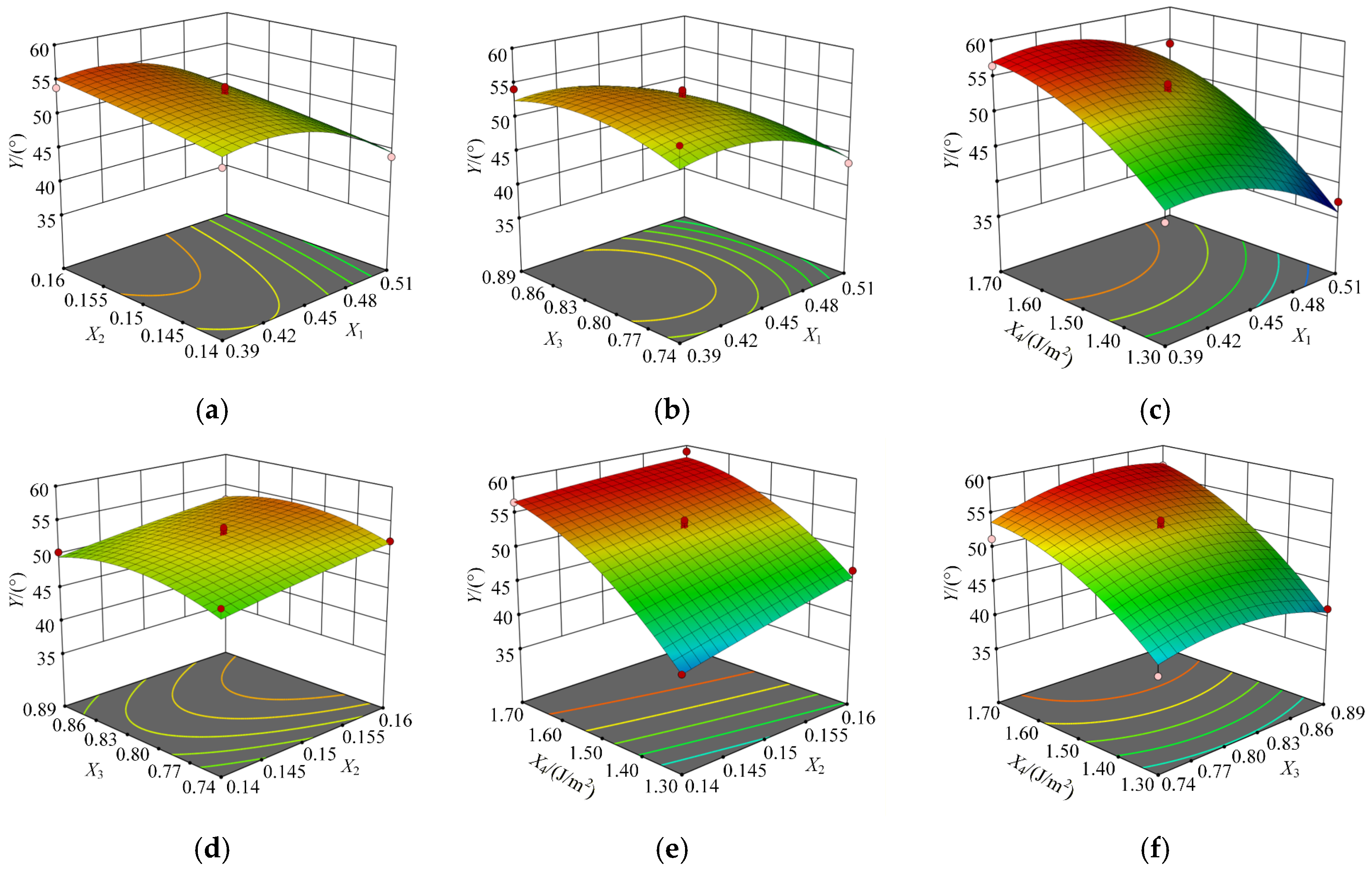
Figure 14 shows the response surfaces depicting the interactions among the coefficient of restitution (X₁), rolling friction coefficient (X₂), static friction coefficient (X₃), and surface energy (X₄). These surfaces are derived from the multiple quadratic regression model. Analysis of these response surfaces reveals the following trends. When the coefficient of restitution (X₁) is held constant, the angle of repose (Y) increases slowly with increasing rolling friction coefficient (X₂) and static friction coefficient (X₃). It increases rapidly with increasing surface energy (X₄). Thus, surface energy (X₄) exerts a stronger influence on angle of repose (Y) than rolling friction coefficient (X₂) and static friction coefficient (X₃). When the rolling friction coefficient (X₂) is fixed, the angle of repose (Y) decreases rapidly with increasing coefficient of restitution (X₁). It increases rapidly with increasing surface energy (X₄) and slowly with increasing static friction coefficient (X₃). Therefore, coefficient of restitution (X₁) and surface energy (X₄) have a stronger effect on angle of repose (Y) than static friction coefficient (X₃). When the static friction coefficient (X₃) is held constant, the angle of repose (Y) decreases rapidly with increasing coefficient of restitution (X₁). It increases slowly with increasing rolling friction coefficient (X₂) and rapidly with increasing surface energy (X₄). Hence, surface energy (X₄) and coefficient of restitution (X₁) have a greater influence on angle of repose (Y) than rolling friction coefficient (X₂). When the surface energy (X₄) is fixed, the angle of repose (Y) increases rapidly with increasing rolling friction coefficient (X₂). It increases slowly with increasing static friction coefficient (X₃) and decreases rapidly with increasing coefficient of restitution (X₁). Thus, coefficient of restitution (X₁) and rolling friction coefficient (X₂) exert a greater effect on angle of repose (Y) than static friction coefficient (X₃). These findings are consistent with the ANOVA results.

2.5.4. Optimization of Contact Parameters and Simulation Verification

The established quadratic regression model was solved by setting the target angle of repose of cotton residues as 47.46°. The constraint functions and optimization objectives are expressed in Equation (17).

$$\left\{\begin{array}{l}\mathrm{target}\mathrm{value}={47.46}^{\circ }\\ \mathrm{s}.\mathrm{t}.\left\{\begin{array}{l}0.39\le X_1\le 0.51\\ 0.14\le X_2\le 0.16\\ 0.74\le X_3\le 0.89\\ 1.30\le X_4\le 1.70\end{array}\right.\end{array}\right.$$

(17)

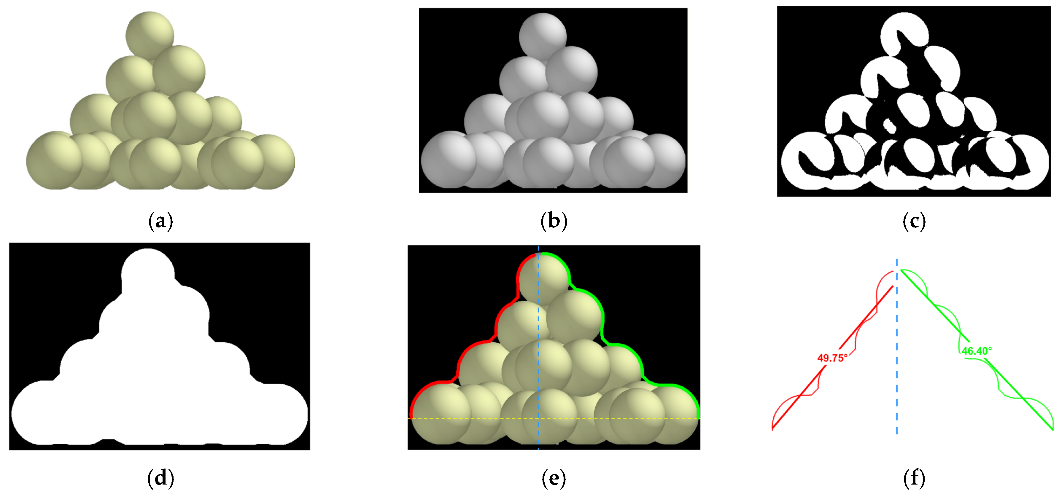
The results showed that the optimal parameter combination was coefficient of restitution of 0.393, rolling friction coefficient of 0.140, static friction coefficient of 0.742, and surface energy of 1.471 J/m². The angle of repose simulation of cotton residues was carried out using the optimized parameters, as shown in Figure 15. Each test was repeated ten times to obtain the average value. The simulated angle of repose was 48.45°, with a relative error of 2.09% compared with the physical test result.

3. Experimental Verification of Vibratory Spreading for Mixed Materials

To further verify the accuracy of intrinsic parameter determination and contact parameter calibration for cotton stalks and cotton residues in the Cotton Stalks and Cotton Residues Mixture, this study developed a dedicated cotton residue recovery device for the mixture. To achieve efficient recovery of large quantities of cotton residues from the mixture, the material first undergoes vibratory dispersion and uniform single-layer spreading. A cotton residue recovery component then collects residues conveyed below the separation box. The spreading completion time and the proportion of cotton residues exposed on the material surface after vibratory spreading were selected as evaluation indexes for the experiment. The proportion of cotton residues exposed on the material surface after vibratory spreading serves as the core verification standard, as it closely aligns with the working mechanism of the residue recovery system. After vibratory spreading, the mixture is transported via a conveyor belt to the area below the separation box. A roller brush inside the box draws surface cotton residues into its interior, and recovery is subsequently achieved through airflow. If cotton residues are buried in the bottom layer by cotton stalks, they cannot be captured by the roller brush, making effective recovery unfeasible. Therefore, the proportion of cotton residues exposed on the material surface after vibratory spreading directly reflects the actual recovery efficiency of the device, and it is the most intuitive and core performance index in this study. In contrast, indexes such as particle distribution uniformity, residence time, and spatial segregation mainly correspond to continuous conveying and screening working conditions. They cannot directly reflect the final recovery effect in the target scenario of this study, so they are not adopted as primary verification indexes.

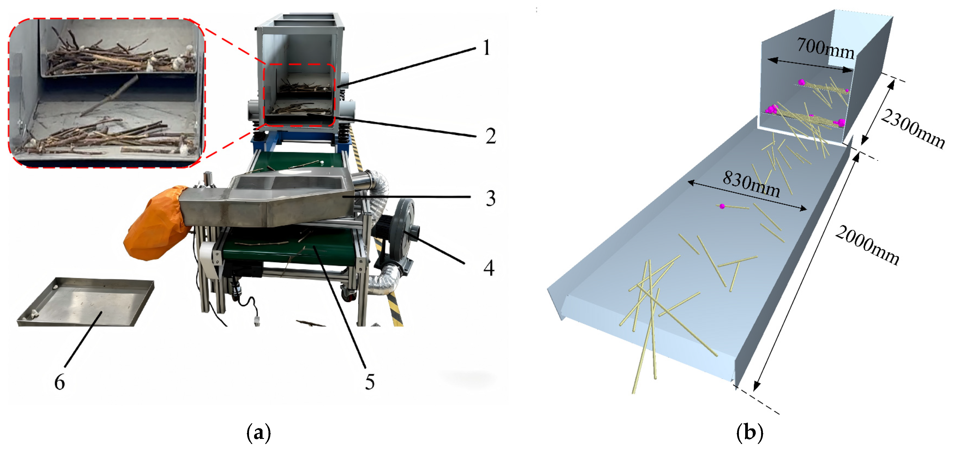
Bench tests and numerical simulations were carried out to verify the prediction performance of the established discrete element model. In both physical bench tests and simulation tests, a total of 4 kg mixed materials were used for each working condition. Each group was repeated three times, and the average value was adopted as the final result. The bench test setup is shown in Figure 16a. In the bench tests, the total mass (m) of cotton residues and the mass exposed on the conveyor surface (m₁) were measured using an electronic balance. In simulation tests, the mass (m₁) was obtained via the post-processing module of EDEM. The surface proportion of cotton residues in both tests was calculated using Equation (18):

$$\eta ={\displaystyle \frac{m_1}{m}}\times 100\%$$

(18)

where η is the proportion of cotton residues on the material surface, in %; m is the total mass of cotton residues in g, and m₁ denotes the mass of surface-exposed cotton residues in g.

For the simulation tests, the corresponding discrete element model was established in EDEM software, and the detailed settings are described as follows. A particle factory with dimensions of 700 mm × 700 mm was established in EDEM software. Cotton stalk and cotton residue particles were generated randomly in accordance with the actual mixing ratio, and the total mass of materials was kept consistent with the physical test. To better replicate the particle size dispersion of real mixed materials, the diameter of each generated particle was set to vary randomly within the range of 0.9–1.1 times the nominal size. Four independent validation working conditions were designed by adjusting the vibration frequency and baffle angle. The fixed basic simulation parameters were set as follows: vibration box inclination of 0°, vibration amplitude of 2 mm, and conveyor speed of 60 mm/s. The specific parameter combinations of each working condition are shown in

Table 12. Comparison of simulation and physical test results under four working conditions.

Test No.	Vibration Frequency (Hz)	Baffle Angle (°)	Simulated Surface Cotton Residue Proportion (%)	Measured Surface Cotton Residue Proportion (%)	Relative Error (%)
1	25	15	97.36	92.87	4.83%
2	30	15	91.15	88.18	3.37%
3	25	13	86.29	82.38	4.75%
4	30	13	82.78	77.59	6.69%

. Continuous vibration loosened and conveyed the mixed materials evenly onto the conveyor belt for subsequent residue recovery. The corresponding simulation model is presented in Figure 16b.

The proportion of cotton residues on the material surface was taken as the core evaluation index to compare the simulation results with the physical test results. The comparison of results under the four working conditions is shown in Table 12.

The mean relative error between simulation and physical test results under the four working conditions is 4.91%. The results indicate that within the tested range of vibration parameters, the discrete element model established in this study achieves acceptable consistency with physical test results. This model can provide a preliminary reference for the structural parameter design of cotton residue separation equipment under similar working conditions.

4. Conclusions

In this study, the intrinsic material parameters of cotton residues were measured via physical experiments. The contact parameters between cotton stalks and cotton residues, as well as between cotton residues and steel, were calibrated by combining physical tests and simulation experiments. Based on the Hertz–Mindlin with JKR contact model, the cohesive contact parameters between cotton residue particles were calibrated with the angle of repose as the response value. Finally, the DEM model was validated through vibratory spreading tests of the cotton stalk and cotton residue mixture, and acceptable agreement between simulation and experimental results was confirmed under the specific material batch, moisture content, and vibratory spreading conditions.

(1) Physical experiments were performed to characterize the basic physical and mechanical parameters of the tested cotton residues in the mixture, including particle size distribution, apparent density, moisture content, shear modulus, and Poisson’s ratio. The measured values under the experimental conditions were 85.43 kg·m⁻³, 5.92%, 3.59 × 10⁻⁶ GPa and 0.36, respectively. The angle of repose of cotton residues was tested via the funnel method, yielding a value of 47.46°.

(2) Combined physical and simulation tests were carried out. Based on the free fall test and inclined plane method, the coefficient of restitution between cotton stalks and cotton residues and between cotton residues and steel were determined as 0.228 and 0.364. The corresponding static friction coefficients were 0.632 and 0.266, and the rolling friction coefficients were 0.199 and 0.156.

(3) The Hertz–Mindlin with JKR contact model was used to calculate the angle of repose formed by falling cotton residue particles. Taking the experimentally measured angle of repose as the target value, the established quadratic regression model was solved. The calibrated internal contact parameters of cotton residues were 0.393 for the coefficient of restitution, 0.140 for the rolling friction coefficient, 0.742 for the static friction coefficient and 1.471 J/m² for the surface energy. Vibratory spreading tests of mixed materials were performed using the calibrated parameters. Under the four sets of vibration parameter conditions, the mean relative error between simulation and bench test results was 4.91%. The results indicate that the discrete element model achieves acceptable consistency with physical test results within the tested range of vibration parameters. The calibrated discrete element parameters are applicable for the simulation of cotton stalk–cotton residue mixture systems under similar working conditions, and the established model can provide a preliminary reference for the structural parameter design of cotton residue separation equipment.

(4) The discrete element parameters calibrated in this study apply only to Xinluzao 48 cotton residues at a moisture content of 5.92%. These parameters may vary with cotton cultivar, harvesting conditions, moisture content, and residue morphology. These uninvestigated factors represent the main limitations of this study. Future work will extend parameter calibration to more cultivars and working conditions to enhance the practical applicability of the DEM model.

References

1. Vitale, G.S.; Scavo, A.; Zingale, S.; Tuttolomondo, T.; Santonoceto, C.; Pandino, G.; Lombardo, S.; Anastasi, U.; Guarnaccia, P. Agronomic Strategies for Sustainable Cotton Production: A Systematic Literature Review. Agriculture 2024, 14, 1597. [Google Scholar] [CrossRef] [Scilit]
2. Elshareef, H.; Yu, Y.H.; Fu, Y.K.; Ren, S.H. Bio-energy potential of cotton stalks via thermal technologies: A review. J. Cotton Res. 2025, 8, 36. [Google Scholar] [CrossRef] [Scilit]
3. Chen, X.; Liu, Z.H.; Chen, W.; Yang, H.P.; Chen, H.P. Catalytic Pyrolysis of Cotton Stalk to Produce Aromatic Hydrocarbons over Fe Modified CaO Catalysts and ZSM-5. J. Anal. Appl. Pyrolysis 2022, 166, 105635. [Google Scholar] [CrossRef] [Scilit]
4. Zhang, Z.J.; Sang, D.J.; Zhang, J.Y.; Su, L.L.; Amat, G.; Hou, L.Z.; Guo, T.J. Effects of Cotton Straw Added to Total Mixed Pelleted Feed on the Composition of Rumen Microbiota in Breeding Ewes. Front. Microbiol. 2025, 16, 1604710. [Google Scholar] [CrossRef] [Scilit] [PubMed]
5. Zhu, S.; Liu, J.; Tang, G.; Sun, T.; Jia, H.; Zhao, H.; Zhang, Y.; Lin, L.; Xu, W. Evaluating the Application Potential of Acid-Modified Cotton Straw Biochars in Alkaline Soils Based on Entropy Weight TOPSIS. Agronomy 2023, 13, 2807. [Google Scholar] [CrossRef] [Scilit]
6. Zhong, P.X.; Chen, P.Y.; Huo, P.J.; Ma, L.; Xu, Z.X.; Li, F.G.; Cai, C.G. Characterization of Cotton Stalk as a Lignocellulosic Feedstock for Single-Cell Protein Production. Bioresour. Technol. 2025, 417, 131797. [Google Scholar] [CrossRef] [Scilit] [PubMed]
7. Zheng, G.; Qi, B.; Zhang, W.; Shao, W.; Zhang, L.; Wang, Y.; Ding, Y. Engineering Discrete Element Method-Based Design and Optimization of the Key Components of a Spoon-Wheel Spinach Seed-Metering Device. Agronomy 2024, 14, 2096. [Google Scholar] [CrossRef] [Scilit]
8. Horabik, J.; Molenda, M. Parameters and contact models for DEM simulations of agricultural granular materials: A review. Biosyst. Eng. 2016, 147, 206–225. [Google Scholar] [CrossRef] [Scilit]
9. Yue, Y.; Zhang, Q.; Dong, B.; Li, J. Application of Discrete Element Method to Potato Harvesting Machinery: A Review. Agriculture 2025, 15, 315. [Google Scholar] [CrossRef] [Scilit]
10. Ai, X.M.; Yi, J.Y.; Pei, Z.S.; Zhou, W.Y.; Feng, D.C. Advances in Discrete Element Modeling of Asphalt Mixture: A Literature Review. Arch. Comput. Methods Eng. 2024, 31, 4003–4029. [Google Scholar] [CrossRef] [Scilit]
11. Liu, G.M.; Yao, J.Y.; Chen, Z.; Han, X.K.; Zou, M. Mesoscopic Analysis of Drag Reduction Performance of Bionic Furrow Opener Based on the Discrete Element Method. PLoS ONE 2023, 18, e0293750. [Google Scholar] [CrossRef] [Scilit] [PubMed]
12. Liang, D.; Liu, W.C.; Zhong, T.H.; Liu, H.; Dhandapani, R.; Li, H.; Wang, J.W.; Wolcott, M. Nanocellulose Reinforced Lightweight Composites Produced from Cotton Waste via Integrated Nanofibrillation and Compounding. Sci. Rep. 2023, 13, 2144. [Google Scholar] [CrossRef] [Scilit] [PubMed]
13. Wang, P.; Wang, H.; Zhang, R.; Hu, R.; Hao, B.; Huang, J. Numerical Simulation of an Online Cotton Lint Sampling Device Using Coupled CFD–DEM Analysis. Agriculture 2024, 14, 127. [Google Scholar] [CrossRef] [Scilit]
14. Lv, H.M.; Ma, C.Q. Experimental Study on the Dielectric Spectrum of Cotton Fiber Aggregation. Adv. Mater. Res. 2013, 821–822, 1475–1478. [Google Scholar] [CrossRef] [Scilit]
15. Manjunath, B.R.; Venkataraman, A. Fibrillar Aggregation in Cotton Cellulose Subjected to Multiple Swelling Treatments with Alkali. J. Polym. Sci. Polym. Chem. Ed. 1980, 18, 1407–1424. [Google Scholar] [CrossRef] [Scilit]
16. Chen, T.; Yi, S.J.; Li, Y.F.; Tao, G.X.; Mao, X. Calibration and Test of Contact Parameters for Alfalfa Stalk at Primary Florescence Based on Discrete Element Method. PLoS ONE 2024, 19, e0303064. [Google Scholar] [CrossRef] [Scilit] [PubMed]
17. Boac, J.M.; Casada, M.E.; Pordesimo, L.O.; Petingco, M.C.; Maghirang, R.G.; Harner, J.P. Evaluation of particle models of corn kernels for discrete element method simulation of shelled corn mass flow. Smart Agric. Technol. 2023, 4, 100197. [Google Scholar] [CrossRef] [Scilit]
18. Yuan, F.; Yu, H.; Wang, L.; Shi, Y.; Wang, X.; Liu, H. Parameter Calibration and Systematic Test of a Discrete Element Model (DEM) for Compound Fertilizer Particles in a Mechanized Variable-Rate Application. Agronomy 2023, 13, 706. [Google Scholar] [CrossRef] [Scilit]
19. Wang, X.; Wu, W.; Jia, H. Calibration of Discrete Element Parameters for Simulating Wheat Crushing. Food Sci. Nutr. 2023, 11, 7751–7764. [Google Scholar] [CrossRef] [Scilit] [PubMed]
20. Jia, H.P.; Feng, B.; Wu, W.B.; Yang, K.X. Discrete Element Method Parameter Calibration and Validation of Wheat Based on the Tavares Model. PLoS ONE 2026, 21, e0346715. [Google Scholar] [CrossRef] [Scilit] [PubMed]
21. Huang, H.; Zhang, Y.; Hou, G.; Su, B.; Yin, H.; Fu, Z.; Zhuang, Y.; Lv, Z.; Tian, H.; Li, L. Establishment of Hollow Flexible Model with Two Types of Bonds and Calibration of the Contact Parameters for Wheat Straw. Agriculture 2025, 15, 1686. [Google Scholar] [CrossRef] [Scilit]
22. Zeng, F.; Diao, H.; Liu, Y.; Ji, D.; Dou, M.; Cui, J.; Zhao, Z. Calibration and Validation of Simulation Parameters for Maize Straw Based on Discrete Element Method and Genetic Algorithm–Backpropagation. Sensors 2024, 24, 5217. [Google Scholar] [CrossRef] [Scilit] [PubMed]
23. Chen, Z.; Che, G.; Wan, L.; Wang, H.; Zhang, K. Calibration and Experimental Validation of Discrete Element Parameters for Long-Grain Rice with Different Moisture Contents Based on Repose Angle. Agriculture 2025, 15, 1058. [Google Scholar] [CrossRef] [Scilit]
24. Qi, B.; Guo, S.; Gao, Y.; Ye, M.; Xie, C.; Zhang, A.; Wu, Y.; Feng, X. Segmental Calibration of Soil–Tool Contact Models for Sustainable Tillage Using Discrete Element Method. Sustainability 2025, 17, 8126. [Google Scholar] [CrossRef] [Scilit]
25. Zhang, X.; Wang, R.; Wang, B.; Chen, J.; Wang, X. Parameter Calibration of Discrete Element Model of Wine Lees Particles. Appl. Sci. 2024, 14, 5281. [Google Scholar] [CrossRef] [Scilit]
26. Peng, F.; Zhang, L.M.; Li, Z.Q.; Chen, J.M. Calibration and Verification of DEM Parameters of Wet-Sticky Feed Raw Materials. Sci. Rep. 2023, 13, 9246. [Google Scholar] [CrossRef] [Scilit] [PubMed]
27. Yu, W.; Liu, R.; Yang, W. Parameter Calibration of Pig Manure with Discrete Element Method Based on JKR Contact Model. AgriEngineering 2020, 2, 25. [Google Scholar] [CrossRef] [Scilit]
28. Campos-M, M.; Campos-C, R. Applications of quartering method in soils and foods. Int. J. Agric. Food Sci. 2017, 7, 235–239. [Google Scholar] [CrossRef] [Scilit]
29. Starkova, O.; Aniskevich, A. Poisson’s Ratio and the Incompressibility Relation for Various Strain Measures with the Example of a Silica-Filled SBR Rubber in Uniaxial Tension Tests. Polym. Test. 2010, 29, 310–318. [Google Scholar] [CrossRef] [Scilit]
30. Sun, J.Y.; Hu, J.L.; Zheng, Z.L.; He, X.T.; Geng, H.H. A Practical Method for Simultaneous Determination of Poisson’s Ratio and Young’s Modulus of Elasticity of Thin Films. J. Mech. Sci. Technol. 2011, 25, 3165–3171. [Google Scholar] [CrossRef] [Scilit]
31. Zhang, J.X.; Zhang, P.; Zhang, H.; Tan, C.L.; Wan, W.Y.; Wang, Y.C. Calibration of Discrete Element Simulation Parameters for Xinjiang Cotton Straw. Trans. Chin. Soc. Agric. Mach. 2024, 55, 76–84, 108. [Google Scholar] [CrossRef]
32. Hertz, H. Ueber die Berührung fester elastischer Körper. J. Reine Angew. Math. 1882, 92, 156–171. [Google Scholar] [CrossRef] [Scilit]
33. Mindlin, R.D. Compliance of elastic bodies in contact. J. Appl. Mech. 1949, 16, 259–268. [Google Scholar] [CrossRef] [Scilit]
34. Chen, X.Y.; Ji, L.Y.; Li, Y. Experimental and Theoretical Analysis of Large Particle–Wall Collision with Different Metal Plates. J. Braz. Soc. Mech. Sci. Eng. 2022, 44, 77. [Google Scholar] [CrossRef] [Scilit]
35. Zhang, S.L.; Zhao, H.B.; Wang, X.Z.; Dong, J.X.; Zhao, P.F.; Yang, F.F.; Chen, X.H.; Liu, F.; Huang, Y.X. Discrete Element Modeling and Shear Properties of the Maize Stubble-Soil Complex. Comput. Electron. Agric. 2023, 204, 107519. [Google Scholar] [CrossRef] [Scilit]
36. Konopka, S.; Kolankowska, E. Methodological Aspects of Determining the Coefficient of Kinetic Friction of Wheat Kernels on an Inclined Plane. Tribologia 2018, 278, 45–50. [Google Scholar] [CrossRef] [Scilit]
37. Jin, Y.; Song, Z.; Zhang, R.; Zhang, J. Experiment and analysis of physical, mechanical, and viscoelastic properties of the roots and stalks of green leafy vegetables. PLoS ONE 2024, 19, e0305572. [Google Scholar] [CrossRef] [Scilit] [PubMed]
38. Roessler, T.; Katterfeld, A. DEM Parameter Calibration of Cohesive Bulk Materials Using a Simple Angle of Repose Test. Particuology 2019, 45, 105–115. [Google Scholar] [CrossRef] [Scilit]
39. Wei, S.X.; Li, B.; Yang, J.X.; Cai, D.S.; Xu, W.B.; Liu, Z.Y. Calibration of Discrete Element Parameters for Cohesive Soils at Different Moisture Contents. PLoS ONE 2026, 21, e0340462. [Google Scholar] [CrossRef] [Scilit] [PubMed]
40. Hu, Z.; Li, H.; Shi, X.; Kong, L.; Tian, X.; An, S.; Feng, B.; Ma, J. Discrete Element Simulation Parameter Calibration of Wheat Straw Feed Using Response Surface Methodology and Particle Swarm Optimization–Backpropagation Hybrid Algorithm. Appl. Sci. 2025, 15, 7668. [Google Scholar] [CrossRef] [Scilit]
41. Hu, Y.; Xiang, W.; Duan, Y.; Yan, B.; Ma, L.; Liu, J.; Lyu, J. Calibration of Ramie Stalk Contact Parameters Based on the Discrete Element Method. Agriculture 2023, 13, 1070. [Google Scholar] [CrossRef] [Scilit]
42. Li, X.; Xu, Y.; Zhou, J.; Wang, H.; Xu, X.; Zuo, J. Calibration and Experiment of Discrete Element Parameters for Mechanically Harvested Dried Saffron Filaments. Trans. Chin. Soc. Agric. Eng. 2026, 42, 150–160. [Google Scholar] [CrossRef]
43. Jiang, W.; Wang, L.; Tang, J.; Yin, Y.; Zhang, H.; Jia, T.; Qin, J.; Wang, H.; Wei, Q. Calibration and Experimental Validation of Contact Parameters in a Discrete Element Model for Tobacco Strips. Processes 2022, 10, 998. [Google Scholar] [CrossRef] [Scilit]
44. Li, J.; Lu, Y.; Peng, X.; Jiang, P.; Zhang, B.; Zhang, L.; Meng, H.; Kan, Z.; Wang, X. Discrete Element Method for Simulation and Calibration of Cotton Stalk Contact Parameters. BioResources 2022, 18, 400–416. [Google Scholar] [CrossRef] [Scilit]
Figure 1. Cotton residues in cotton fields and mechanically harvested cotton stalk–cotton residue mixture. (a) Cotton residues in cotton fields; (b) Mechanically harvested cotton stalks mixed with cotton residues.
Agriculture 16 01492 g001
Figure 2. Tensile Tests of Cotton Residues. (a) Tensile test of cotton residues; (b) Force-displacement curve of cotton residues.
Agriculture 16 01492 g002
Figure 3. Development of Discrete Element Models for Cotton Stalks and Cotton Residues. (a) Discrete element model of cotton stalks; (b) Discrete element model of cotton residues.
Agriculture 16 01492 g003
Figure 4. DEM computational model. (a) Hertz–Mindlin contact model; (b) Particle motion calculation model. Note: kn is the normal stiffness, N/m; kt is tangential stiffness, N/m; Cn is normal damping, N·s/m; Ct is tangential damping, N·s/m; μ is the friction coefficient; Fn is the normal force, N; Ft is the tangential force, N.
Agriculture 16 01492 g004
Figure 5. Physical test for measuring the coefficients of restitution. (a) Cotton residues–Cotton stalks; (b) Cotton residues–Steel.
Agriculture 16 01492 g005
Figure 6. Simulation test of coefficients of restitution. (a) Cotton stalks–Cotton residues; (b) Cotton residues–Steel.
Agriculture 16 01492 g006
Figure 7. Fitted curves of coefficient of restitution from simulation tests.
Agriculture 16 01492 g007
Figure 8. Physical and simulation tests of static friction coefficient between materials. (a) Physical test of cotton residues–steel; (b) Physical test of cotton residues–cotton stalks; (c) Simulation test of cotton residues–steel; (d) Simulation test of cotton residues–cotton stalks. 1. Fixed material friction surface; 2. Sliding material friction surface; 3. Fixed support; 4. Angle measuring instrument; 5. Rotating inclined plane.
Agriculture 16 01492 g008
Figure 9. Fitted curves of static friction coefficient from simulation tests.
Agriculture 16 01492 g009
Figure 10. Physical and simulation tests of rolling friction coefficient between materials. (a) Physical test of cotton residues–steel; (b) Physical test of cotton residues–cotton stalks; (c) Simulation test of cotton residues–steel; (d) Simulation test of cotton residues–cotton stalks. 1. Spacer block; 2. Material sample plate; 3. Support; 4. Angle measuring instrument; 5. Inclined plane.
Agriculture 16 01492 g010
Figure 11. Fitted curves of rolling friction coefficient from simulation tests.
Agriculture 16 01492 g011
Figure 12. Angle of repose test of cotton residues. (a) Physical test of cotton residues angle of repose; (b) Simulation test of cotton residues angle of repose.
Agriculture 16 01492 g012
Figure 13. Extraction of the Angle of Repose. (a) Original image; (b) Grayscale image; (c) Binary image; (d) Morphological operations; (e) Extract boundary curves; (f) Linear fitting. Note: The red lines represent the left contour of the material and its corresponding fitted straight line, while the green lines represent the right contour of the material and its corresponding fitted straight line.
Agriculture 16 01492 g013
Figure 14. Response surfaces of interaction effects of contact parameters on the angle of repose. (a) Interaction effect of X1 and X2 on Y; (b) Interaction effect of X1 and X3 on Y; (c) Interaction effect of X1 and X4 on Y; (d) Interaction effect of X2 and X3 on Y; (e) Interaction effect of X2 and X4 on Y; (f) Interaction effect of X3 and X4 on Y.
Agriculture 16 01492 g014
Figure 15. Angle of repose extraction from simulation tests. (a) Original image; (b) Grayscale image; (c) Binary image; (d) Morphological operations; (e) Extract boundary curves; (f) Linear fitting. Note: The red lines represent the left contour of the material and its corresponding fitted straight line, while the green lines represent the right contour of the material and its corresponding fitted straight line.
Agriculture 16 01492 g015
Figure 16. Validation of vibrating spreading test for mixed materials: (a) Bench test of vibrating spreading for mixed materials; (b) Simulation test of vibrating spreading for mixed materials. 1. Vibrating box; 2. Material baffle; 3. Sorting box; 4. Fan; 5. Material conveyor belt; 6. Cotton residues collection box.
Agriculture 16 01492 g016