Dual-Model Assessment of Ecosystem Respiration Using Random Forest and Lloyd–Taylor Models in Two High-Altitude Agricultural River Basins: Spatiotemporal Dynamics

Abstract

The alpine valley agricultural region is the most intensively human-impacted ecosystem type on the Qinghai–Tibet Plateau, and its ecosystem respiration (RE) plays an important role in regional carbon cycling and climate change responses. However, it remains unclear whether systematic differences exist in the spatiotemporal patterns of RE and its environmental controls across high-altitude agricultural watersheds. Using multi-source remote sensing and reanalysis data from 2000 to 2024, this study focuses on two representative valley agricultural basins on the Qinghai–Tibet Plateau—the Huangshui River Basin (HSH) and the Yijianglianghe River (YJLH). A dual-model framework combining a Random Forest model and a Lloyd–Taylor mechanistic model was developed to examine the spatiotemporal dynamics, driving mechanisms, and temperature sensitivity of RE. The results show that RE increased in both basins over the study period, while their dominant controlling mechanisms differed markedly. Gross primary productivity (GPP) was the most important driver in both basins (23.6% in HSH and 24.5% in YJLH). However, temperature and precipitation contributed more in YJLH (14.5% vs. 9.4%), suggesting that RE in the higher-altitude basin is more strongly constrained by hydrothermal conditions under colder and harsher climates. Spatially, high RE values in the HSH were mainly concentrated in mid- and low-elevation valley farmlands, whereas the YJLH exhibited a clear decrease in RE with increasing elevation, indicating a stronger topographic control. Both basins showed significant spatial clustering of RE (Moran’s I ≈ 0.93), with stronger spatial aggregation in the HSH. Temperature sensitivity (Q₁₀) generally increased with elevation, and the YJLH exhibited markedly higher Q₁₀ values in high-altitude regions, indicating stronger temperature responsiveness under extreme cold conditions. Empirical Q₁₀ values were consistently higher than theoretical estimates, implying that ecosystem respiration is not only directly driven by temperature, but may also be amplified indirectly through enhanced vegetation productivity and increased substrate availability. Overall, this study reveals a clear divergence in RE control mechanisms across valley agricultural systems on the Qinghai–Tibet Plateau: productivity-driven regulation dominates in low-elevation regions, whereas hydrothermal constraints become increasingly important in high-altitude environments, leading to a transition from “productivity control” to “hydrothermal constraint control.” This shift highlights the nonlinear response of alpine agroecosystems to elevation gradients and climate change, providing mechanistic evidence for understanding carbon cycling in high-altitude anthropogenic ecosystems.

1. Introduction

Ecosystem respiration (RE) represents the primary pathway through which terrestrial ecosystems return CO₂ to the atmosphere, with an annual flux of approximately 100–120 Pg C, making it the second largest terrestrial carbon flux after gross primary productivity (GPP) [1,2,3]. Soil respiration (Rs) accounts for 60–80% of RE, reaching 80–100 Pg C yr⁻¹, roughly 8–10 times current global fossil fuel emissions [4,5]. Because RE responds sensitively to temperature, even modest warming can substantially alter atmospheric CO₂ growth rates and terrestrial carbon sink strength [1,6]. Accurate characterization of RE spatiotemporal patterns, driving mechanisms, and long-term trends is therefore fundamental to understanding climate–carbon cycle feedbacks and evaluating carbon mitigation outcomes [4,5,6].

Agricultural ecosystems play a distinctive and complex role in the global carbon cycle. Cropland covers approximately 12% of the Earth’s land surface, and soil carbon emissions from these systems account for an estimated 14% to 24% of total anthropogenic greenhouse gas emissions [4,7]. Management practices such as fertilization, irrigation, and tillage markedly elevate both the baseline rate and the temperature sensitivity of soil respiration in agricultural ecosystems by increasing soil organic matter input and enhancing microbial activity [8,9,10]. Global-scale meta-analyses indicate that experimental warming increases cropland soil CO₂ emissions by approximately 15% on average, an enhancement that consistently exceeds values reported for most natural ecosystems [8,9]. Concurrently, land-use change also substantially alters soil carbon emission processes, with large-magnitude effects on soil respiration rate [10,11,12,13]. Nevertheless, compared with forest and grassland ecosystems, long-term observations and regional-scale modelling of RE in agricultural ecosystems remain markedly insufficient. The spatial and temporal patterns and environmental drivers of soil respiration in high-altitude agricultural valleys, in particular, are still poorly understood. In these settings, extreme environmental conditions—low temperatures, intense radiation, and short growing seasons—intersect with intensive anthropogenic management, potentially generating carbon cycling patterns distinct from those of natural ecosystems. Research addressing these high-altitude systems, however, remains exceedingly scarce.

The Qinghai–Tibetan Plateau (QTP), often termed the “Third Pole,” ranks among the most climate-sensitive regions on Earth [14,15,16]. Over the past five decades, the QTP has warmed at 0.3–0.4 °C decade⁻¹, markedly exceeding the global mean, with pronounced elevation-dependent warming [17,18]. The plateau’s extensive permafrost and alpine meadows store vast quantities of soil organic carbon, comparable in magnitude to Arctic permafrost carbon pools [19,20]. High-altitude ecosystems exhibit elevated temperature sensitivity: low-temperature environments yield higher apparent activation energies for carbon decomposition, driving Q₁₀ values well above the global average [20,21]. Consequently, even modest temperature changes can trigger substantial carbon flux responses. Chen et al. (2013) reviewed evidence that sustained warming has already enhanced net primary productivity and soil respiration across the plateau, while permafrost thaw and glacial retreat continue to mobilize long-sequestered organic carbon, raising concerns about the stability of the QTP carbon sink [14].

The QTP has long been regarded as an important terrestrial carbon sink. Wei et al. (2021) estimated, on the basis of eddy covariance measurements, that plateau ecosystems absorb approximately 178–318 Tg C annually, with most observation sites functioning as net carbon sinks [19]. Recent evidence, however, suggests that warming-driven RE enhancement may progressively erode this sink capacity. Shen et al. (2026) employed a knowledge-guided deep neural network to project that under SSP5-8.5, increased RE could offset roughly 70% of the current plateau carbon sink, with some regions at risk of transitioning from net sink to net source [21]. Process-based simulations further indicate that future permafrost degradation will expose substantial soil organic carbon to decomposition, amplifying heterotrophic respiration [22]. Carbon sink stability has thus emerged as a central concern in QTP carbon cycle research [22,23].

Among the natural ecosystems that dominate the Qinghai–Tibet Plateau, valley agricultural areas constitute a relatively distinctive yet long-underestimated component of the regional carbon cycle. Although cropland in these valleys accounts for only approximately 1% of the total plateau area, it supports the vast majority of the human population and agricultural activity, and represents one of the most concentrated sources of anthropogenic carbon emissions on the plateau [24,25]. Against this backdrop, the Huangshui River Basin (HSH) and the Yijiang–Lianghe River Basin (YJLH) were selected as representative study areas to characterize the spatial heterogeneity and contrasting environmental responses of ecosystem respiration (RE) across valley agricultural ecosystems of the Qinghai–Tibet Plateau. The HSH, situated on the northeastern margin of the plateau, is strongly influenced by the East Asian monsoon, has a relatively humid climate, a long history of agricultural development, and high intensity of human activity. The YJLH, located in the south–central plateau, lies at higher elevation with a colder, more arid climate, and is dominated by a mosaic of alpine valley agriculture and grassland. These two basins thus exhibit clear gradients in hydrothermal conditions, elevation, and anthropogenic pressure. Ecologically, both basins lie within the core distribution zone of valley agriculture on the Qinghai–Tibet Plateau, yet they differ markedly in land-use composition, cropping structure, and degree of human disturbance, together representing different stages of the transition from relatively intensive agriculture to semi-natural farming systems. Furthermore, each basin encompasses a pronounced altitudinal gradient, producing a characteristic “valley–alpine slope” composite landscape that provides a natural control for examining the response mechanisms of ecosystem respiration under contrasting environmental constraints. Compared with the surrounding high-altitude meadows and desert ecosystems, valley agricultural areas feature higher mean annual temperatures, longer growing seasons, and stronger anthropogenic disturbance. Consequently, their carbon cycling processes are characterized by greater spatial heterogeneity and more complex patterns of environmental response [11,26,27,28]. Prior work has demonstrated that agricultural inputs and land-use change markedly enhance regional greenhouse gas emissions and alter the balance between carbon sequestration and release [29,30]. Nevertheless, research on ecosystem respiration across the Qinghai–Tibet Plateau remains concentrated on alpine grasslands, permafrost, and other natural ecosystems. Systematic understanding of the long-term spatiotemporal dynamics and driving mechanisms of RE in valley agricultural areas remains notably limited.

To address uncertainties in ecosystem respiration (RE) dynamics across alpine valley agricultural systems on the Qinghai–Tibetan Plateau, particularly the relative contributions of climatic forcing, vegetation productivity, and topographic heterogeneity, we developed a dual-model framework that integrates data-driven and process-based approaches. The Random Forest (RF) model serves as a statistical upscaling tool that captures nonlinear spatiotemporal variability in RE and its associations with multiple environmental predictors [31,32,33], with SHAP (SHapley Additive exPlanations) analysis used to quantify the contributions and nonlinear interactions of environmental variables [34]. In parallel, a mechanistic model (MECH) based on the Lloyd–Taylor temperature response formulation provides a process-constrained benchmark representing temperature-dependent respiration dynamics [35,36,37]. The comparison between RF and MECH is not intended as an equivalence test between two models of the same class. Rather, it constitutes a complementary model intercomparison designed to evaluate structural consistency, to quantify uncertainty arising from empirical versus process-based representations, and to assess the extent to which observed RE patterns can be reproduced under differing modeling assumptions. SHAP (SHapley Additive exPlanations) analysis was applied to interpret the RF-derived relationships by quantifying the marginal contributions and nonlinear effects of individual environmental variables, thereby improving mechanistic interpretability and identifying the dominant statistical controls on RE variability [34]. Within this framework, climatic variables are treated as external environmental forcing, vegetation productivity as a proxy for ecosystem carbon supply capacity, and anthropogenic influence as a representation of land-use intensity regulating ecosystem conditions. The study is structured around three objectives: (i) to quantify the spatiotemporal heterogeneity of RE and its environmental associations using RF; (ii) to disentangle the roles of climatic forcing, vegetation productivity, and anthropogenic regulation in shaping RE variability across contrasting valley systems; and (iii) to evaluate the temporal evolution, elevation-dependent patterns, and temperature sensitivity of RE. The third objective distinguishes long-term climate-driven changes from spatial variability in environmental regulation and assesses the implications for carbon cycling under ongoing warming, with a comparative focus on two representative agricultural valley basins on the Qinghai–Tibetan Plateau.

2. Materials and Methods

2.1. Study Area

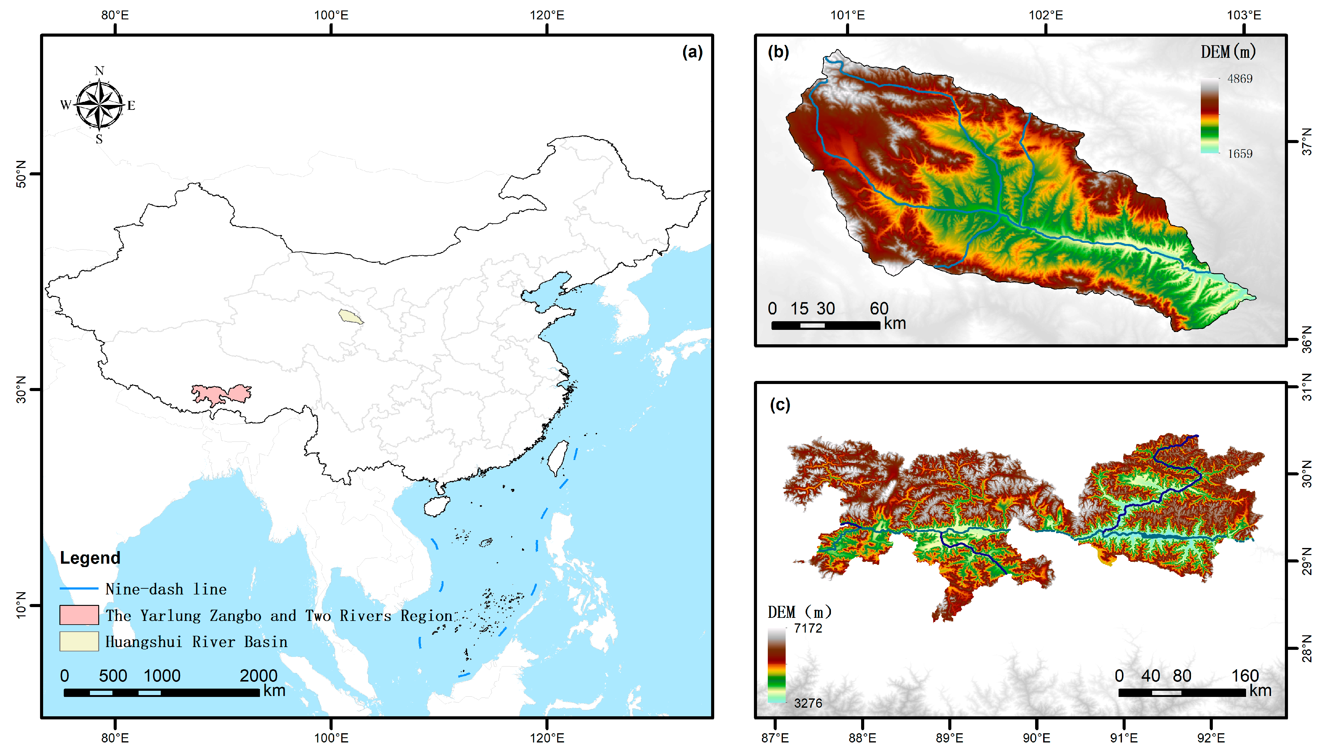
This study focused on two representative valley agricultural basins on the QTP: the Huangshui River Basin (HSH) and the Yijianglianghe River Basin (YJLH) (Figure 1). Located in the northeastern margin and south–central plateau, respectively, these two basins encompass pronounced differences in physical geography while both supporting concentrated human activity, making them well suited for characterizing spatial variation in alpine ecosystem processes and land-use patterns under contrasting topographic and climatic settings.

The Huangshui River Basin (HSH, 100.68–103.07° E, 36.03–37.47° N) covers approximately 1.6 × 10⁴ km², with elevations ranging from 1650 to 4850 m. The climate is semi-arid continental plateau, with a mean annual temperature (MAT) of approximately 8.1 °C and mean annual precipitation (MAP) of 300–500 mm, concentrated in summer. Vegetation is dominated by temperate steppe and shrubland, with cropland distributed extensively along valley floors and alpine meadow and bare land occupying higher elevations. Terrain relief is substantial, with deep river incision producing pronounced valley–ridge contrasts. Cropland, settlements, and transportation networks cluster along valley bottoms and river terraces in a marked riparian corridor pattern, forming a typical agro-pastoral ecotone in the northeastern QTP.

The Yijianglianghe River Basin (YJLH, 87.08–92.62° E, 28.28–30.48° N) covers approximately 7.5 × 10⁴ km², with elevations from 3300 to 7100 m. The climate is alpine semi-arid, with MAT of approximately 6.2 °C and MAP of 200–400 mm. Vegetation consists mainly of alpine steppe and alpine meadow, with limited cropland and wetland along valley bottoms and alpine desert and ice cover at high elevations. The elevation gradient spans nearly 4000 m from valley floor to summit, producing strong vertical zonation. Agriculture and settlements concentrate along the Yarlung Zangbo River and its tributaries, where relatively flat terrain and favorable thermal conditions prevail, making the YJLH one of the most important valley agricultural areas in the south–central QTP. The steep elevation gradient and diverse ecological zones also render this basin an ideal setting for studying carbon cycle responses to climate change in high-altitude ecosystems.

In summary, the HSH and YJLH represent two distinctive valley agricultural systems in the northeastern and south–central QTP, respectively. Both basins exhibit strong dependence of ecological patterns and land use on valley topography, hydrothermal conditions, and elevation gradients, yet they differ substantially in climatic background, geomorphological structure, vegetation composition, and regional context. These contrasts provide an ideal comparative framework for examining ecological processes and environmental responses across distinct QTP valley systems.

2.2. Data Sources

The datasets used in this study comprise remote sensing products, reanalysis data, and a digital elevation model, spanning 2000–2024. All data layers were preprocessed and resampled to 1 km spatial resolution in the WGS84 geographic coordinate system (EPSG:4326). Data sources are summarized in

Table 1. Data sources used in this study.

Data	Source	Native Resolution
Precipitation	National Tibetan Plateau Data Center (https://data.tpdc.ac.cn, accessed on 1 November 2025)	1 km
Temperature	National Tibetan Plateau Data Center (https://data.tpdc.ac.cn, accessed on 1 November 2025)	1 km
GloFlux (RE)	National Tibetan Plateau Data Center (https://data.tpdc.ac.cn, accessed on 1 November 2025)	1 km
Soil moisture (0–7 cm)	ERA5-Land reanalysis (https://cds.climate.copernicus.eu, accessed on 1 November 2025)	1 km
Soil temperature (0–7 cm)	ERA5-Land reanalysis (https://cds.climate.copernicus.eu, accessed on 1 November 2025)	1 km
Solar radiation	ERA5-Land reanalysis (https://cds.climate.copernicus.eu, accessed on 1 November 2025)	1 km
EVI	MODIS MOD13A2 (https://lpdaac.usgs.gov/products/mod13a2v061/, accessed on 1 November 2025)	1 km
Daytime LST	MODIS MOD11A2 (https://lpdaac.usgs.gov/products/mod11a2v061/, accessed on 1 November 2025)	1 km
Nighttime LST	MODIS MOD11A2 (https://lpdaac.usgs.gov/products/mod11a2v061/, accessed on 1 November 2025)	1 km
NDVI	MODIS MOD13A3 (https://lpdaac.usgs.gov/products/mod13a3v061/, accessed on 1 November 2025)	1 km
GPP	MODIS MOD17A2H (https://lpdaac.usgs.gov/products/mod17a2hv061/, accessed on 1 November 2025)	1 km
DEM	NASADEM (https://lpdaac.usgs.gov/products/nasadem_hgtv001/, accessed on 1 November 2025)	30 m
Land cover	CLCD (https://zenodo.org/records/5816591, accessed on 1 November 2025)	30 m

.

The ecosystem respiration (RE) data used in this study was obtained from the GloFlux dataset provided by the National Tibetan Plateau Data Center (https://data.tpdc.ac.cn). GloFlux is a machine-learning-based global carbon flux product that integrates in situ flux tower observations (e.g., FLUXNET, AmeriFlux and ICOS) [38], satellite remote sensing data, and meteorological reanalysis data to generate spatially continuous estimates of key ecosystem carbon fluxes at 0.1° resolution for 2000–2024. The RE component represents ecosystem respiration (RECO) derived from this data-fusion modeling framework rather than direct field measurements. As a hybrid observational–modeling product, GloFlux has been validated against independent flux tower data and shows robust performance across multiple ecosystem types. In this study, it is used as a reference dataset for model training and calibration, while acknowledging that it inherits uncertainties from both the underlying observations and the upscaling procedure.

All datasets used in this study were harmonized to a consistent spatial framework to ensure compatibility across multi-source variables. MODIS products (e.g., NDVI, EVI, GPP, and land surface temperature) and TPDC ecosystem respiration (RE) data were originally provided at 1 km spatial resolution, whereas ERA5-Land reanalysis data were provided at 0.1° (~9–10 km at the study latitude). To ensure spatial alignment across all predictor and response variables, ERA5-Land datasets were resampled to a 1 km grid using bilinear interpolation. It is important to emphasize that this resampling procedure does not increase the intrinsic spatial information content of the original ERA5-Land data. The effective spatial resolution of these variables remains constrained by their native ~10 km scale, and the resampled fields should be interpreted as spatially continuous representations of coarse-resolution signals rather than fine-scale observations. To avoid potential overinterpretation of artificially enhanced spatial detail, all analyses involving ERA5-Land variables were evaluated with consideration of spatial autocorrelation. In particular, statistical significance was interpreted using effective degrees of freedom adjusted according to spatial dependence structure. Additionally, to assess the robustness of spatial patterns, key analyses were repeated under aggregated resolutions (5 km and 10 km), and results showed consistent spatial trends, indicating that the main conclusions are not sensitive to the choice of resampling scale. This multi-scale consistency check confirms that the adopted 1 km harmonized framework provides a computationally consistent and analytically stable basis for integrating heterogeneous geospatial datasets, without introducing spurious fine-scale spatial structure.

2.3. Methods

2.3.1. Random Forest Model

A Random Forest (RF) model was employed to predict monthly ecosystem respiration (RE) [39,40]. The model used 11 environmental variables as predictors, with GloFlux RE as the target variable. Model hyperparameters were set as follows: number of trees (n_estimators) = 500, minimum samples per leaf (min_samples_leaf) = 5, maximum features (max_features) = ‘sqrt’, out-of-bag estimation enabled (oob_score = True), and random state = 42.

To rigorously evaluate model generalization, we applied grouped K-fold cross-validation (GroupKFold, k = 5) with grouping by year, ensuring that all months within a given year belonged to the same fold. This strategy prevented information leakage from temporal autocorrelation. Each training fold sampled at most 125,000 pixels (maximum 5000 per year) to maintain spatial representativeness. Model performance was assessed using the cross-validation coefficient of determination (CV R²), root mean square error (RMSE), and out-of-bag R² (OOB R²). Separate models were trained for the HSH and YJLH to capture basin-specific environmental controls on RE.

2.3.2. Lloyd–Taylor Mechanistic Model and Rref Calibration

A mechanistic model (MECH) based on the Lloyd–Taylor equation was constructed for comparison with the machine learning model. This model partitions ecosystem respiration into autotrophic and heterotrophic components:

$$RE=\mathrm{a}\times GPP+R_{ref}\times \exp \left(E_0\times \left({\displaystyle \frac{1}{T_{ref}-T_0}}-{\displaystyle \frac{1}{T-T_0}}\right)\right)$$

(1)

Here, the term a × GPP represents the autotrophic respiration component, where a is an empirical parameter adopted from previous studies [41]. The second term describes the heterotrophic respiration component, with the temperature response modelled using the Lloyd–Taylor equation. The parameters are as follows: E₀ = 308.56 K (activation energy), T₀ = −46.02 °C, T_ref = 15 °C (reference temperature), and T denotes all-day land surface temperature (LST) [35,41].

R_ref (gC m⁻² month⁻¹) denotes the reference respiration rate at the reference temperature T_ref = 15 °C. A key challenge for valley agricultural systems on the Qinghai–Tibet Plateau is the absence of in situ flux tower observations in both basins. To address this, we developed an indirect calibration strategy. The independent GloFlux product [42] was used as an observational constraint to invert the Lloyd–Taylor equation, and pixel-level Rref estimates were then aggregated into a single effective Rref for each basin using robust statistical methods. The underlying assumption of this indirect calibration is that GloFlux, although derived primarily from machine-learning upscaling of literature-based eddy covariance measurements rather than from direct observations within the HSH or YJLH, provides an unbiased estimate of the regional ecosystem respiration (RE) magnitude. The calibrated Rref values therefore align the Lloyd–Taylor model with the best currently available independent RE product, while the median-based aggregation approach effectively reduces the influence of errors at the individual pixel level. The calibration results are presented in

Table 2. Model performance, parameter calibration, and dual-model consistency assessment.

Model Index	HSH	YJLH
CV R2 (mean ± std)	0.887 ± 0.011	0.613 ± 0.014
CV Pearson r	0.942	0.784
CV RMSE (g C·m−2·month−1)	0.514	0.369
CV Bias (g C·m−2·month−1)	0.002	0.003
OOB R2	0.908	0.626
Rref Median	1.639	1.026
Rref 25th percentile	0.894	0.625
Rref 75th percentile	3.315	1.622
Rref Mean	2.210	1.229
Calibration sample size (N)	744,257	2,751,030
Number of calibration months	40	40
Dual-model Pearson r	0.864	0.874
Dual-model RMSE (g C·m−2·month−1)	0.880	0.290

.

2.3.3. SHAP Explainability Analysis

To reveal the contribution mechanisms of individual predictors to RE predictions, SHAP (SHapley Additive exPlanations) analysis was applied [42,43]. SHAP values, rooted in Shapley values from cooperative game theory, quantify the marginal contribution of each feature to individual predictions. The trained RF model was loaded with shap.TreeExplainer, and SHAP values were computed for approximately 2000 randomly sampled data points. Mean |SHAP| served as the global feature importance metric, and SHAP dependence plots visualized nonlinear response relationships between features and RE.

$$RE(x^{(i)})={\phi }_0+{\displaystyle \sum _{j=1}^{11}{\phi }_j}(x^{(i)})$$

(2)

$${\varphi }_j\left(x^{(i)}\right)={\displaystyle \sum _{S\subseteq N\backslash \left\{j\right\}}\frac{\left|S\right|!(11-|S|-1)!}{11!}} [ E\left[f(X)\mid do(X_{S\cup \left\{j\right\}})\right]-E\left[f(X)\mid do(X_S)\right] ]$$

(3)

$$E\left[f(X)\mid do\left(X_S=x_S^{(i)}\right)\right]={\displaystyle \int f}\left(x_S^{(i)}, X_{\overline{S}}\right) dP\left(X_{\overline{S}}\right)$$

(4)

$$I_j={\displaystyle \frac{1}{n}}{\displaystyle \sum _{i=1}^n|}{\varphi }_j(x^{(i)})|,j=1,2,\dots ,11$$

(5)

The RF-predicted RE for any pixel i is fully decomposed into a baseline value φ₀—the mean RF prediction over all training samples—and the sum of SHAP contributions φ_j from the 11 features. A positive φ_j (>0) indicates that the feature drives RE upward, whereas a negative φ_j (<0) indicates suppression. φ_j is defined as follows. Over all feature subsets S that do not contain j (2¹⁰ possible subsets in total), a weighted average is computed of the change in the expected model prediction when j becomes known, relative to knowing only the features in S. The weighting scheme ensures that every feature ordering is treated equally. The operator do(·) denotes an intervention: the values of the known features are fixed at their observed values, while the remaining features are randomly drawn from their marginal distribution. This severs the confounding influence of collinearity among features. The features belonging to subset S are fixed at the observed values of pixel i, denoted $x_S^{(i)}$, while the remaining features $x_{\overline{S}}$ are randomly drawn from the background marginal distribution $P{x}_{\overline{S}}$ and integrated over.

2.3.4. Mann–Kendall Trend Test and Sen’s Slope Estimation

Pixel-wise Mann–Kendall (MK) trend tests and Sen’s slope estimation were applied to characterize spatiotemporal trends in RE over 2000–2024 [44,45]. For each pixel, a 25-year RE time series was constructed. The MK test statistic S, its variance Var(S), and the standardized test statistic Z were computed following standard formulations. Two-tailed p-values were derived from the standard normal cumulative distribution function. Sen’s slope was defined as the median of all pairwise slopes.

$$S={\displaystyle \sum _{i=1}^{n-1}{\displaystyle \sum _{j=i+1}^n\mathrm{sign}}}(X_j-X_i)$$

(6)

$$\mathrm{Var}(S)={\displaystyle \frac{n(n-1)(2n+5)}{18}}$$

(7)

$$Z=\left\{\begin{array}{ll}\hfill {\displaystyle \frac{S-1}{\sqrt{Var(S)}}} \hfill & S>0\hfill \\ \hfill 0 \hfill & S=0\hfill \\ \hfill {\displaystyle \frac{S+1}{\sqrt{Var(S)}}} \hfill & S<0\hfill \end{array}\right.$$

(8)

$$p=2\left(1-\mathsf{\Phi }(|Z|)\right)$$

(9)

$$\beta =\mathrm{median}\left({\displaystyle \frac{X_j-X_i}{j-i}}\right),\hspace{1em}1\le i<j\le n$$

(10)

2.3.5. Spatial Autocorrelation Analysis

Global Moran’s I was calculated to evaluate spatial autocorrelation of RE [46,47]. The spatial weight matrix was constructed using Rook contiguity (4-neighbor), where only the four orthogonal adjacent pixels in the grid were considered. Moran’s I was computed following:

$$I={\displaystyle \frac{n}{W}}\cdot {\displaystyle \frac{{\displaystyle \sum _{i=1}^n{\displaystyle \sum _{j=1}^n{w}_{ij}}}(x_i-\overline{x})(x_j-\overline{x})}{{\displaystyle \sum _{i=1}^n{(x_i-\overline{x})}^2}}}$$

(11)

$$E[I]=-{\displaystyle \frac{1}{n-1}}$$

(12)

2.3.6. Elevation Gradient Analysis

The DEM was resampled to match the RE grid via bilinear interpolation [48,49]. Elevation bands were delineated at 100 m intervals, and RE statistics (mean, standard deviation) were computed for each band, with a minimum of 30 valid pixels per band. Linear regression of band-mean RE against band-mean elevation yielded elevation lapse rates (g C·m⁻²·month⁻¹ per 100 m) and associated correlation coefficients. Interannual RE trends were further analyzed by elevation band to assess elevation-dependent climate responses.

2.3.7. Q₁₀ Temperature Sensitivity Analysis

Q₁₀, defined as the factor by which RE increases per 10 °C rise in temperature, was calculated from both theoretical and empirical perspectives. Theoretical Q₁₀ was derived from the Lloyd–Taylor equation [50]:

$$Q_{10\mathrm{theor}}=\exp \left({\displaystyle \frac{10E_0}{(T+46.02)(T+56.02)}}\right)$$

(13)

where E₀ = 308.56 K, T is the local mean annual temperature (°C), and T₀ = −46.02 °C. Theoretical Q₁₀ depends solely on local mean temperature and reflects purely thermodynamic temperature sensitivity. Empirical Q₁₀ (RF) was obtained by regressing ln(RE) against temperature T per pixel [51]:

$$\ln (RE)=a+bT$$

(14)

$$Q_{10\mathrm{RF}}=\exp (10b)$$

(15)

Q₁₀ values were constrained to the range [0.5, 10]. The spatial distribution of Q₁₀, its relationship with mean annual temperature, and its variation along the elevation gradient were analyzed.

3. Results

3.1. Random Forest Model Performance and Variable Importance

The RF model achieved strong predictive performance against the independent TPDC RE target (Table 2). For the HSH, CV R² = 0.887 ± 0.011 (OOB R² = 0.908); for the YJLH, CV R² = 0.613 ± 0.014 (OOB R² = 0.626). The lower R² in the YJLH reflects greater spatial heterogeneity and stronger nonlinearity in environmental controls at extreme high elevations.

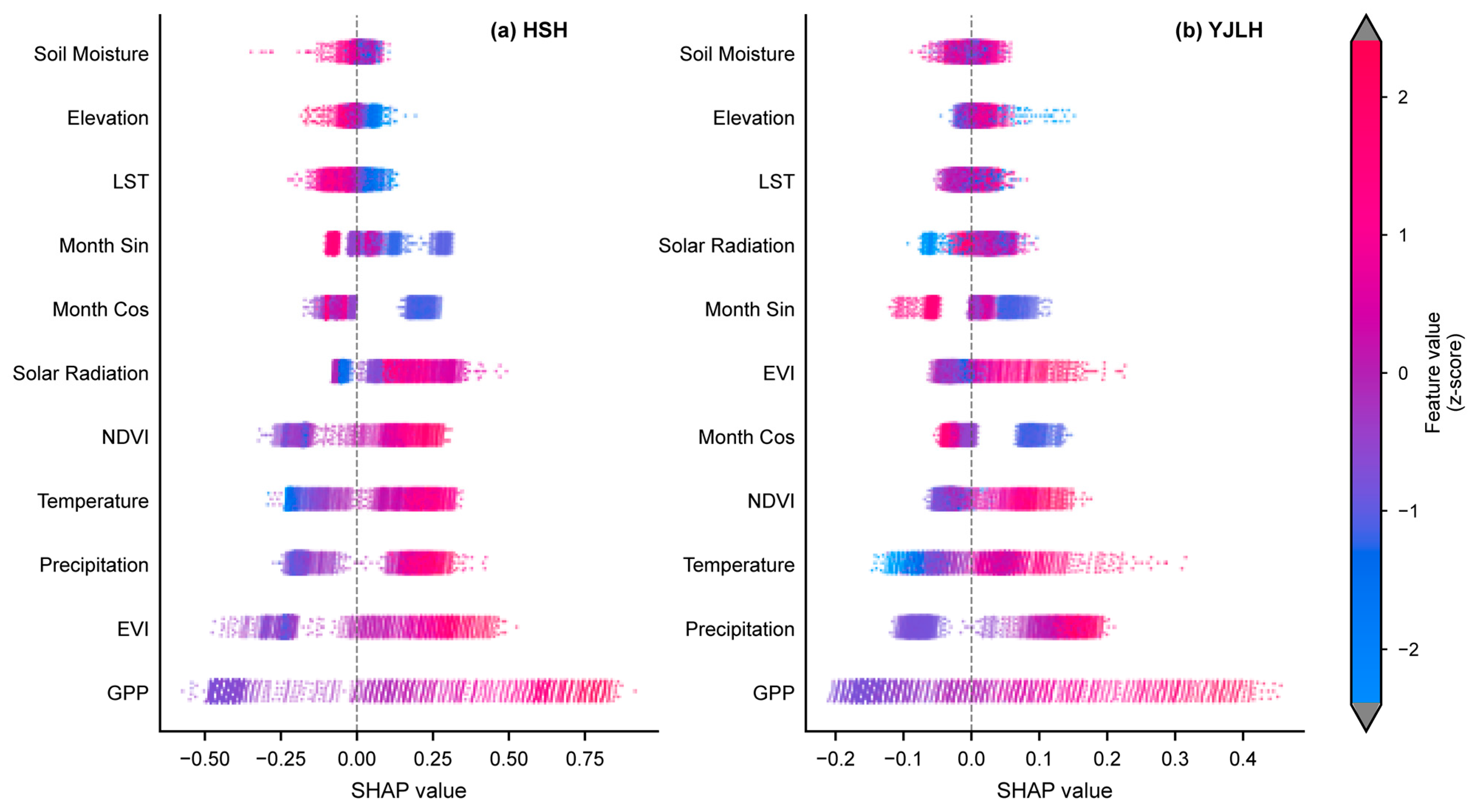
Variable importance analysis (

Table 3. Random Forest variable importance ranking.

Rank	Variable (HSH)	Importance (%)	Variable (YJLH)	Importance (%)
1	GPP	23.6	GPP	24.5
2	Precipitation	18.6	Precipitation	17.5
3	EVI	16.3	Temperature	14.5
4	NDVI	14.5	EVI	10.0
5	Temperature	9.4	NDVI	9.7
6	Solar Radiation	7.5	Solar Radiation	5.7
7	Month_Cos	3.7	Month_Sin	4.1
8	Month_Sin	3.2	Month_Cos	3.8
9	Soil Moisture	1.2	Soil Moisture	3.5
10	Elevation	1.1	Elevation	3.4
11	LST_Day	1.0	LST_Day	3.2

) identified GPP as the single most important predictor in both basins (23.6–24.5%), with precipitation ranking second (17.5–18.6%), consistent with the moisture-limited character of semi-arid plateau ecosystems. Vegetation indices (EVI + NDVI) contributed a combined 19.9–30.8%. Temperature was more important in the YJLH (14.5%) than in the HSH (9.4%). SHAP analysis (Figure 2 and Figure 3) confirmed positive associations of RE with GPP, precipitation, and vegetation greenness.

SHAP analysis further resolved local and global feature contributions. In the HSH, high GPP and EVI values drove marked increases in RE, whereas soil temperature and seasonal terms exhibited complex nonlinear relationships (Figure 2a). In the YJLH, similarly, high GPP and precipitation promoted RE, but temperature effects showed greater heterogeneity (Figure 2b), indicating that local climatic conditions and vegetation status jointly shape the spatial variability of RE across the basin.

3.2. Dual-Model Consistency Assessment

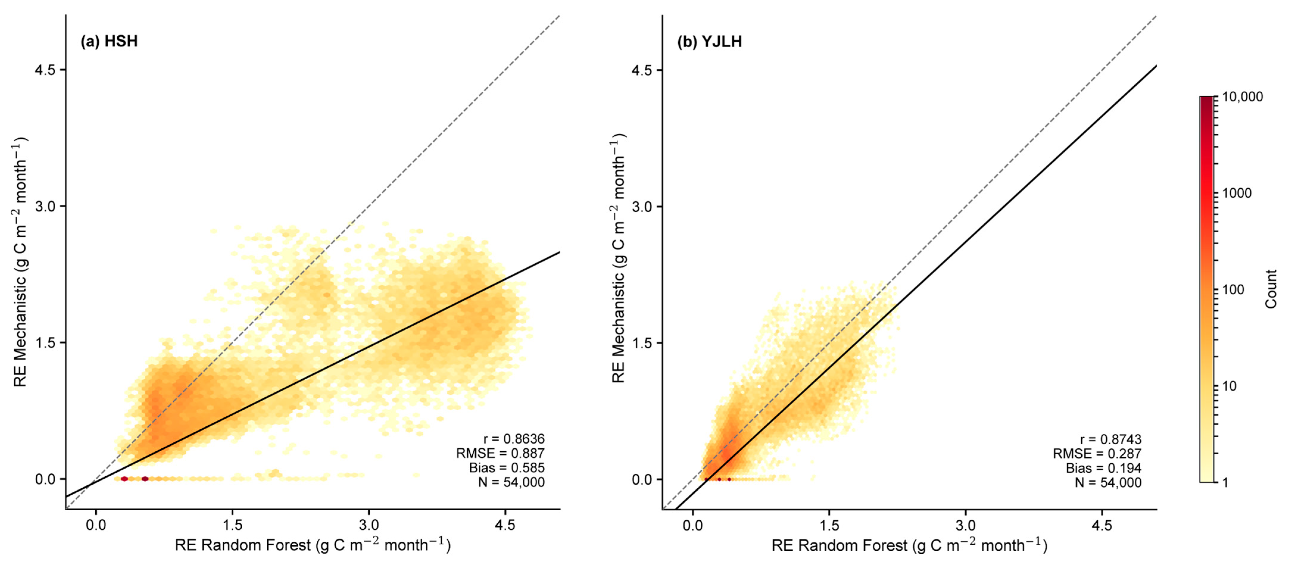
We evaluated the performance of the RF model against the mechanistic model (MECH) for predicting monthly RE and compared their spatial distributions. In the YJLH, the two models produced highly consistent RE spatial patterns (Figure 3b; Pearson r = 0.874, RMSE = 0.287 g C·m⁻²·month⁻¹, Bias = 0.194 g C·m⁻²·month⁻¹), and the scatter density plot showed most predictions distributed near the 1:1 line. In the HSH, the correlation was similarly strong (r = 0.864; Figure 3a), but prediction error was larger (RMSE = 0.887 g C·m⁻²·month⁻¹, Bias = 0.585 g C·m⁻²·month⁻¹), with high-RE regions deviating from the 1:1 line and suggesting systematic overestimation in certain areas.

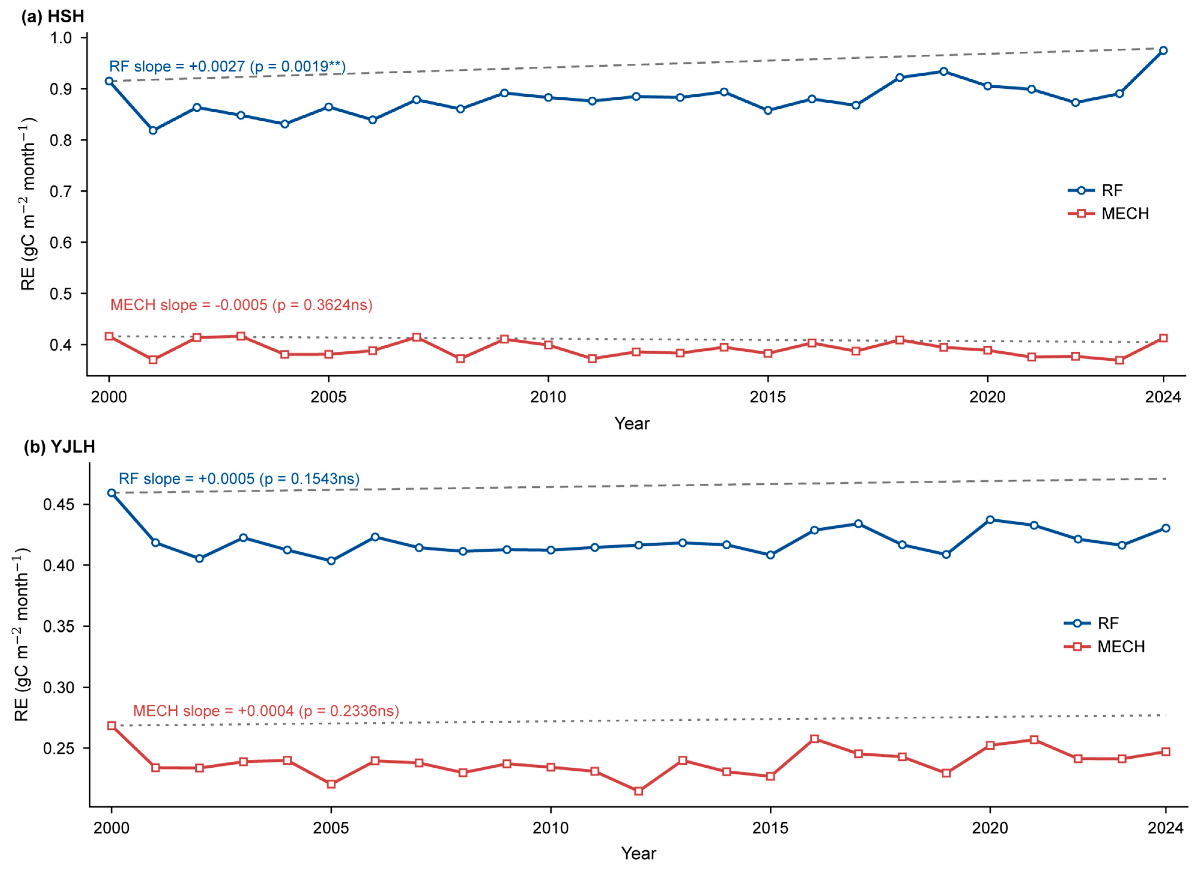
Interannual RE trends from the two models are shown in Figure 4. Both models captured stable interannual fluctuations, but the RF model consistently estimated higher RE levels than MECH across both basins. In the HSH (Figure 4a), RF-simulated RE ranged from 0.82 to 0.98 g C·m⁻²·month⁻¹ and showed a significant increasing trend (slope = +0.0027 yr⁻¹, p = 0.0019), with a sustained rise after 2017 and a peak in 2024. In contrast, MECH estimates were considerably lower (0.37–0.42 g C·m⁻²·month⁻¹) and exhibited no significant trend (slope = −0.0005 yr⁻¹, p = 0.3624), suggesting that the mechanistic model may underestimate RE responses to climate variability and environmental heterogeneity in the HSH.

In the YJLH (Figure 4b), RF-simulated RE was relatively stable (0.40–0.46 g C·m⁻²·month⁻¹), with a weak, non-significant increase (slope = +0.0005 yr⁻¹, p = 0.1543). MECH estimates ranged from 0.22 to 0.26 g C·m⁻²·month⁻¹, also without a significant trend (slope = +0.0004 yr⁻¹, p = 0.2336). Interannual variability in the YJLH was smaller than in the HSH, indicating relatively stable RE in this basin.

The systematic offset between models (RF > MECH) was more pronounced in the HSH. This pattern supports the inference that RF more sensitively captures the effects of climate variability, vegetation dynamics, and topographic heterogeneity on RE, whereas the mechanistic model, constrained by parameterization and process simplification, may underestimate actual carbon release in complex alpine basins.

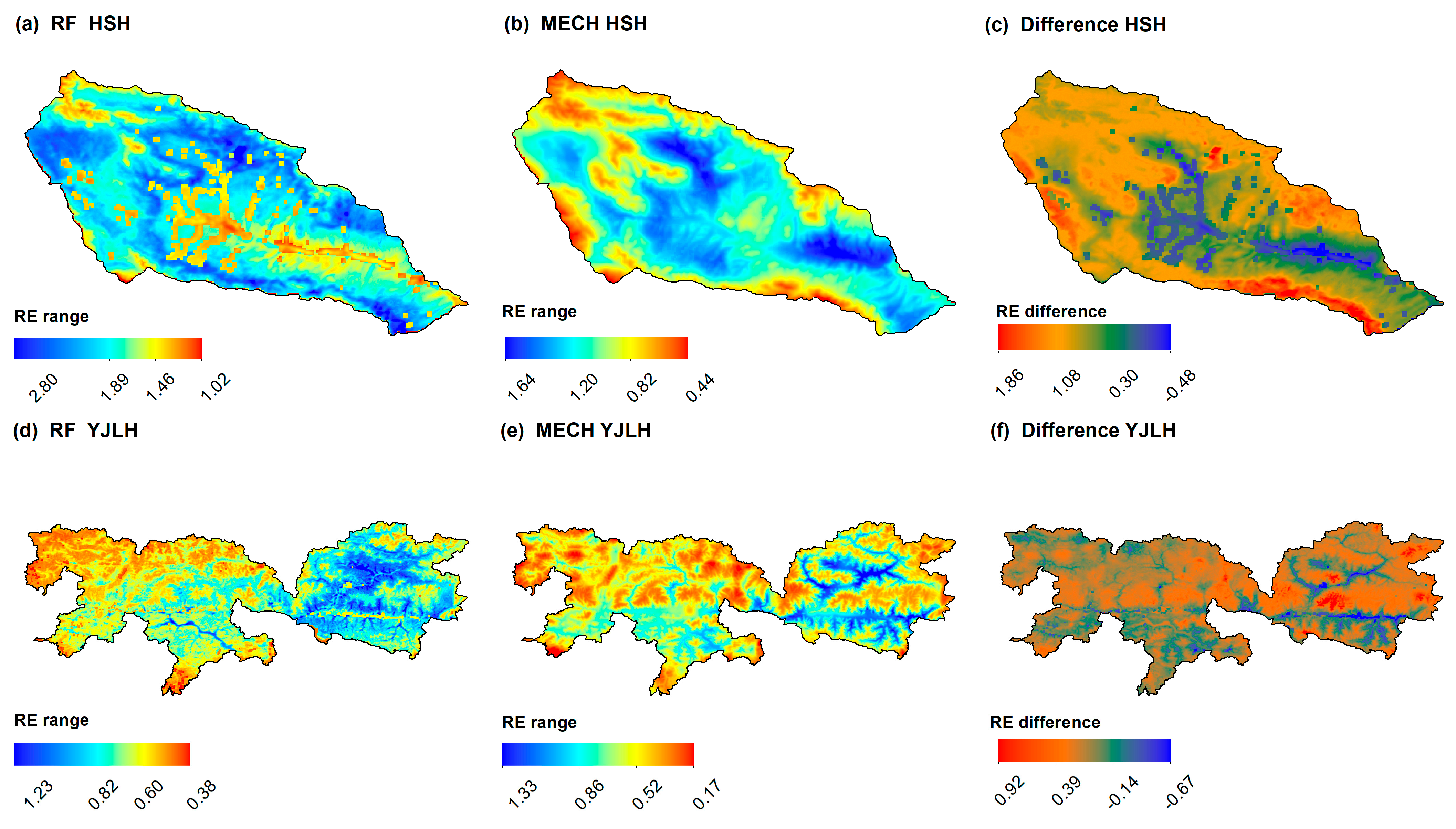
Spatially, in the HSH (Figure 5a–c), the RF model simulates high RE values predominantly in the hilly and mountainous areas of the mid-to-upper watershed, whereas low values concentrate in high-altitude cold regions. The MECH model, by contrast, captures the broad spatial gradient but produces weaker local differentiation and a more continuous spatial pattern. The difference map (RF − MECH) reveals positive values across most of the basin, with differences concentrated mainly in the range of 0.30–1.08 gC m⁻² month⁻¹, indicating that RF predicts higher RE than MECH over the majority of the region. The most pronounced discrepancies occur in the southern basin and parts of the mid-to-lower watershed. Negative values appear only in a few high-altitude areas, suggesting that RF predictions fall slightly below those of MECH under low-temperature conditions.

In the YJLH (Figure 5d–f), both models exhibit clear spatial differentiation. RF simulates high-RE areas primarily in the valley bottoms and low-elevation zones, with lower RE across high-altitude mountainous areas. MECH likewise reproduces the overall spatial gradient, but the extent of high-value areas is smaller and the spatial variation more uniform. The difference map indicates that RF predictions are slightly higher than MECH predictions across most of the basin, with differences concentrated in the range of 0–0.39 gC m⁻² month⁻¹, a smaller overall magnitude than that observed in the HSH. Negative RF − MECH values occur in parts of the high-altitude mountains.

Overall, the RF model resolves the spatial heterogeneity of RE in these high-altitude basins in greater detail, with more pronounced spatial variation in regions of complex topography and steep environmental gradients. The MECH model, constrained by its parameterisation process, produces generally smoother simulations and is less effective in capturing localised high-RE zones. This contrast is more marked in the HSH.

3.3. Spatiotemporal Evolution of Ecosystem Respiration

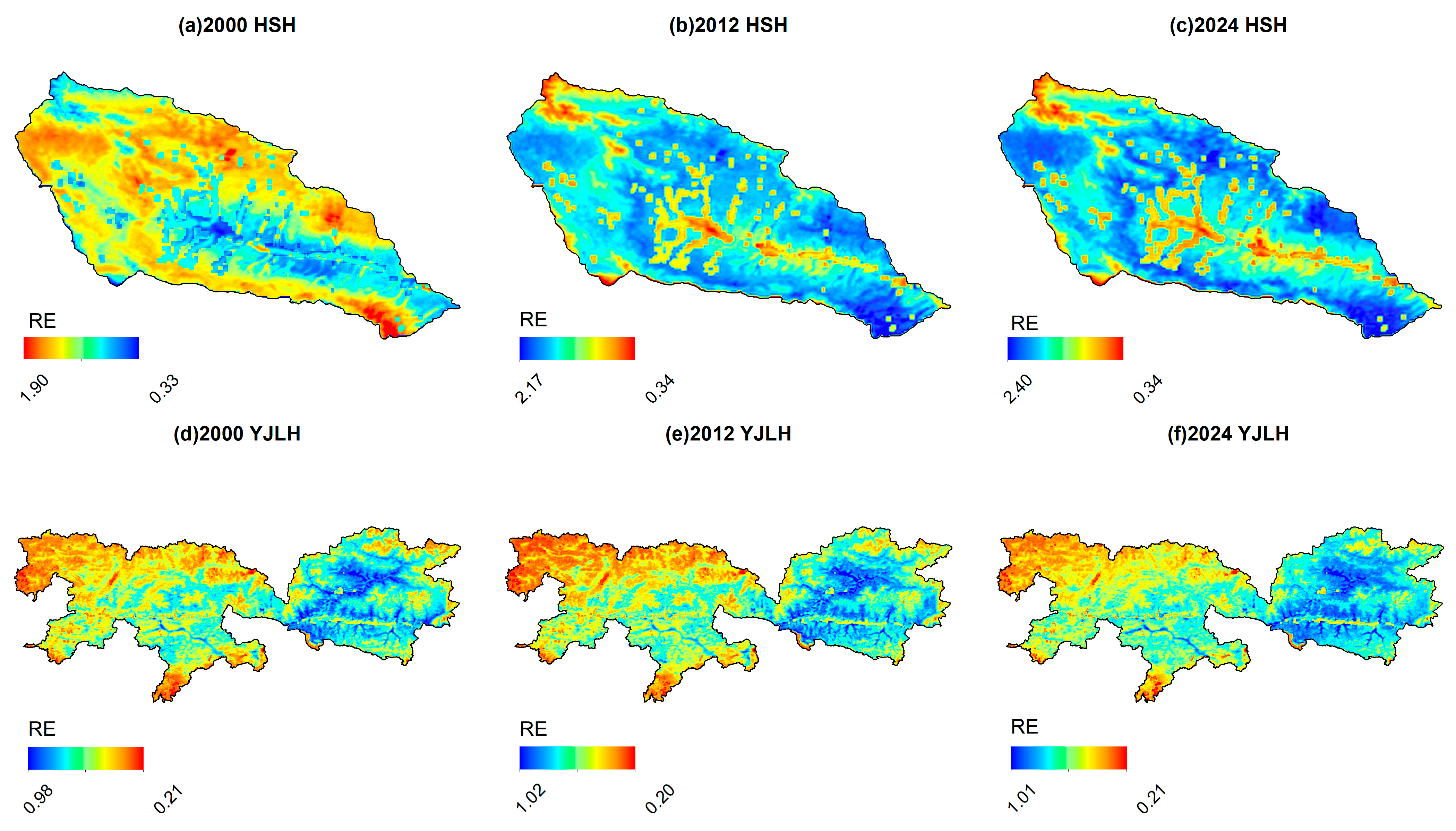
Both basins exhibited pronounced spatial heterogeneity in RE over 2000–2024 (Figure 6), with varying degrees of increasing trend whose magnitude and spatial pattern differed substantially between basins.

Spatially, RE in both basins showed strong elevation gradient effects (Figure 6). In the HSH, high RE values concentrated in mid-to-lower-valley and hilly zones, while southeastern high-elevation mountains maintained lower values. The extent of high-RE areas gradually expanded over the study period, particularly in valley and low-elevation zones; changes in high-elevation areas were weaker, indicating persistent low-temperature limitation. In the YJLH, RE exhibited stronger spatial differentiation, with a general west–high, east–low pattern. High values clustered in valley and low-elevation zones, while alpine zones remained consistently low. Although the overall spatial pattern was stable across years, some valley areas showed increases after 2012.

Interannual analysis (Figure 4) confirmed increasing RE trends in both basins, with stronger changes in the HSH. In the HSH (Figure 4a), RE showed a gradual increase, with a multi-year mean of 0.880 g C·m⁻²·month⁻¹ and a coefficient of variation (CV) of 5.35%. RE fluctuated modestly during 2001–2015, then rose after 2016 and peaked around 2020. In the YJLH (Figure 4b), RE was more stable (mean = 0.418 g C·m⁻²·month⁻¹, CV = 2.98%), with a weaker increase and limited change at the highest elevations.

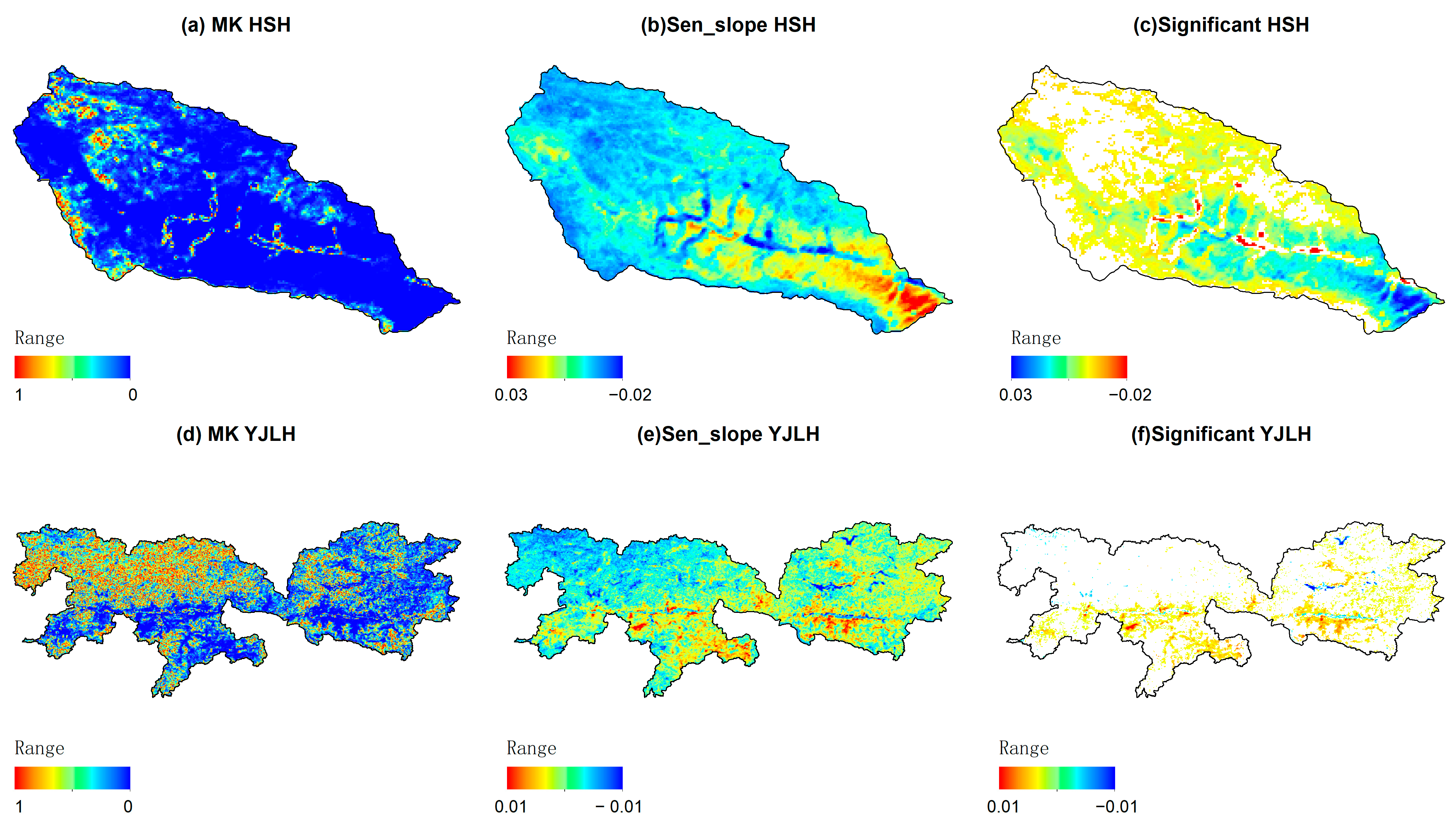
Pixel-wise Mann–Kendall tests and Sen’s slope analysis (Figure 7) further resolved the spatial structure of RE trends. In the HSH (Figure 7a–c), positive MK statistics dominated, with significant increases concentrated in mid-to-lower-valley and hilly zones (local slopes reaching 0.03 yr⁻¹), whereas high-elevation areas showed weaker or slightly negative trends. Regions passing the p < 0.05 threshold were concentrated in valley and low-elevation zones, indicating robust increases there.

In the YJLH (Figure 7d–f), increases predominated but with smaller magnitude. Most Sen’s slopes fell between −0.01 and 0.01 yr⁻¹, and the largest increases occurred in valley and low-elevation zones. Significant increases (p < 0.05) were limited to certain valley areas, whereas large expanses of high-elevation terrain exhibited no significant change.

Overall, RE increases in both basins were concentrated in low-elevation and valley zones, with limited change at high elevations, reinforcing the conclusion that thermal conditions remain the primary constraint on RE in alpine ecosystems. The stronger RE increase and broader spatial extent of significant trends in the HSH indicate greater climate sensitivity in this relatively lower-elevation basin.

3.4. Ecosystem Respiration Across Land-Use Types

RE differed markedly among land-use types, with stronger differentiation in the HSH than in the YJLH (

Table 4. Ecosystem respiration characteristics by land-use type.

Land-Use Type	HSH RE (g C·m−2·Month−1)	YJLH RE (g C·m−2·Month−1)
Cropland	0.477–2.131	0.370–0.993
Forest	0.639–1.953	0.611–0.803
Shrub	0.803–2.100	0.520–0.874
Grassland	0.340–2.115	0.204–0.995
Water Body	0.902–1.741	0.215–0.854
Snow	0.422–1.646	0.227–0.833
Barren	—	—
Impervious	0.806–1.716	—

). In the HSH, cropland (0.477–2.131 g C·m⁻²·month⁻¹), shrubland (0.803–2.100 g C·m⁻²·month⁻¹), and grassland (0.340–2.115 g C·m⁻²·month⁻¹) exhibited the highest RE. Forest and wetland also maintained elevated values, while barren and snow-covered areas were consistently low. In the YJLH, RE levels were generally lower across all land-use types, with most below 1.0 g C·m⁻²·month⁻¹. Grassland and cropland dominated regional RE, whereas alpine barren and snow-covered areas remained low throughout the study period.

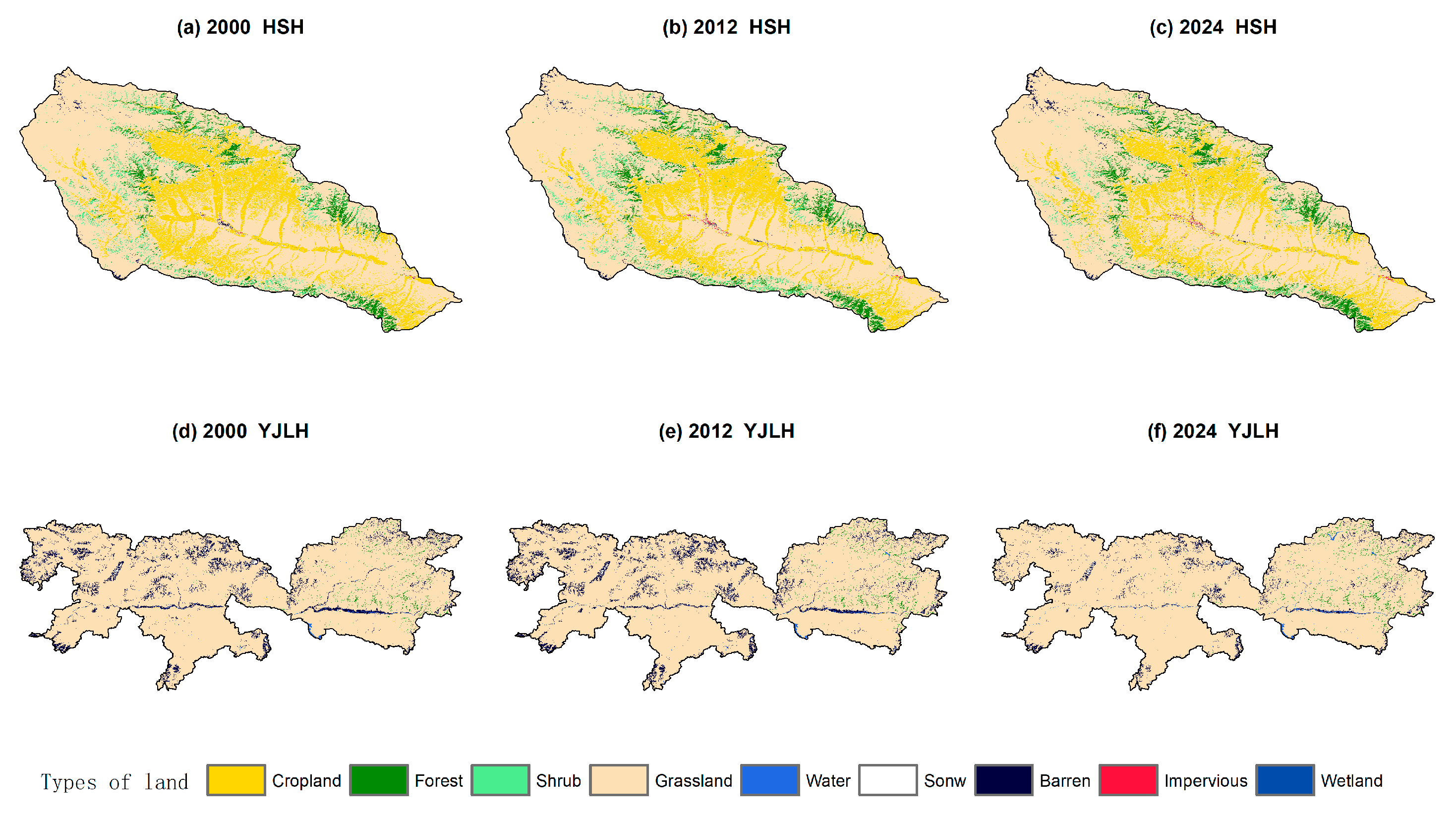
Land-use patterns further shaped the spatial distribution of RE (Figure 8). The HSH was dominated by grassland and cropland, with cropland concentrated along valleys and mid-to-low elevations, broadly coinciding with RE hotspots. Forest and shrubland contributed to local high values in mountain–valley transitions. The YJLH exhibited a simpler land-use composition: grassland dominated, forest and cropland were limited, and high-elevation barren and snow-covered areas were extensive, consistent with the overall lower RE. RE hotspots in the YJLH were restricted to valley and localized low-elevation zones.

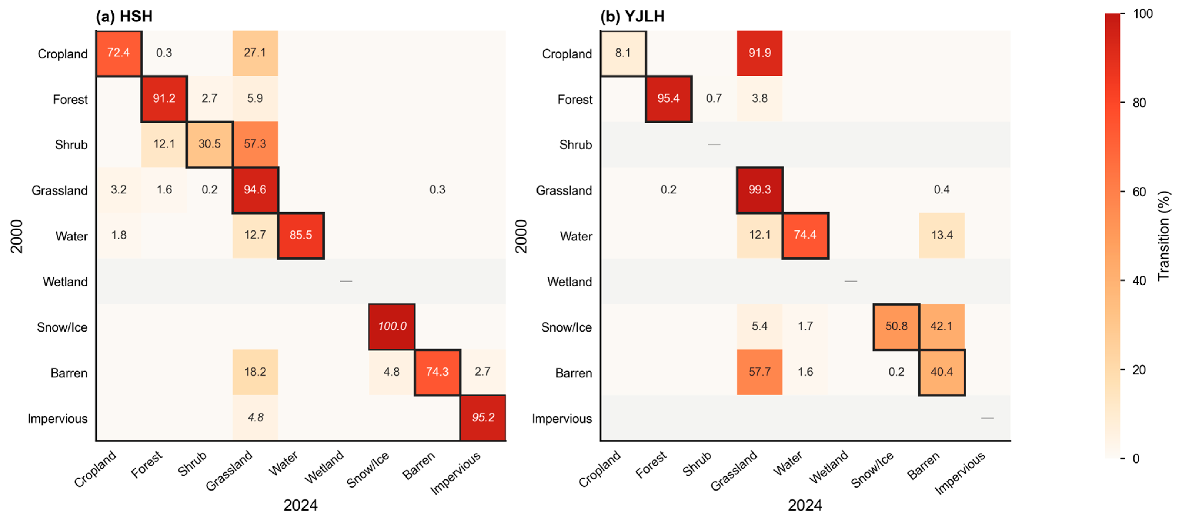
Land-use patterns remained broadly stable over 2000–2024, although local adjustments occurred (Figure 9). In the HSH, grassland maintained dominance, and cropland distribution in valleys remained stable. Forest and shrubland expanded modestly in some mountain and valley-margin areas, while high-elevation barren and snow-covered zones changed little. In the YJLH, alpine grassland remained the dominant type, with minimal spatial reorganization. Cropland and wetland distribution in valleys was stable, but some high-elevation areas showed snow-cover retreat and a corresponding increase in barren ground.

In summary, land-use type was an important control on RE spatial differentiation. Higher vegetation cover (cropland, shrubland, grassland) generally corresponded to higher RE, whereas barren and snow-covered areas remained low. Land-cover changes in alpine zones—particularly snow retreat and local vegetation adjustment—also influenced long-term RE dynamics to some degree.

3.5. Spatial Autocorrelation and Elevation Gradient of RE

During the period 2000–2024, ecosystem respiration (RE) in both the HSH and the YJLH exhibited pronounced spatial autocorrelation. Moran’s I remained consistently high in both basins, indicating that the spatial distribution of RE was strongly clustered rather than random.

In the HSH (

Table 5. Global Moran’s I spatial autocorrelation statistics.

Moran’s I Statistic	HSH	YJLH
Mean ± Std	0.931 ± 0.002	0.930 ± 0.002
Range	[0.927, 0.932]	[0.924, 0.934]
CV (%)	0.19	0.23
p value	<0.001	<0.001
Analysis period	25 years (2000–2024)	25 years (2000–2024)
Adjacency method	Rook (4-neighbor)	Rook (4-neighbor)

), the mean Moran’s I over 2000–2024 was 0.931 ± 0.002, with a range of 0.927–0.934 and a coefficient of variation (CV) of only 0.19%. In the YJLH, the mean Moran’s I was 0.930 ± 0.002, ranging from 0.924 to 0.934, with a CV of 0.23%. All years in both basins passed the significance test (p < 0.001), indicating that RE maintained a stable and significant spatial clustering pattern throughout the study period. Overall, Moran’s I in the HSH was slightly higher than that in the YJLH, suggesting a somewhat stronger degree of spatial continuity and aggregation.

Interannual fluctuations in Moran’s I were small in both basins, indicating that the spatial structure of RE remained generally stable over the study period. This persistent spatial autocorrelation reflects the joint control of ecosystem respiration by regional environmental conditions, including topography, climate, and vegetation distribution. Specifically, low-elevation valley areas consistently formed high-value clusters, whereas high-altitude cold regions formed low-value clusters. Across both basins, RE displayed a highly stable and statistically significant spatial autocorrelation pattern, suggesting that the spatial distribution of ecosystem respiration is under persistent control by regional environmental factors and is characterized by a well-defined spatial organization.

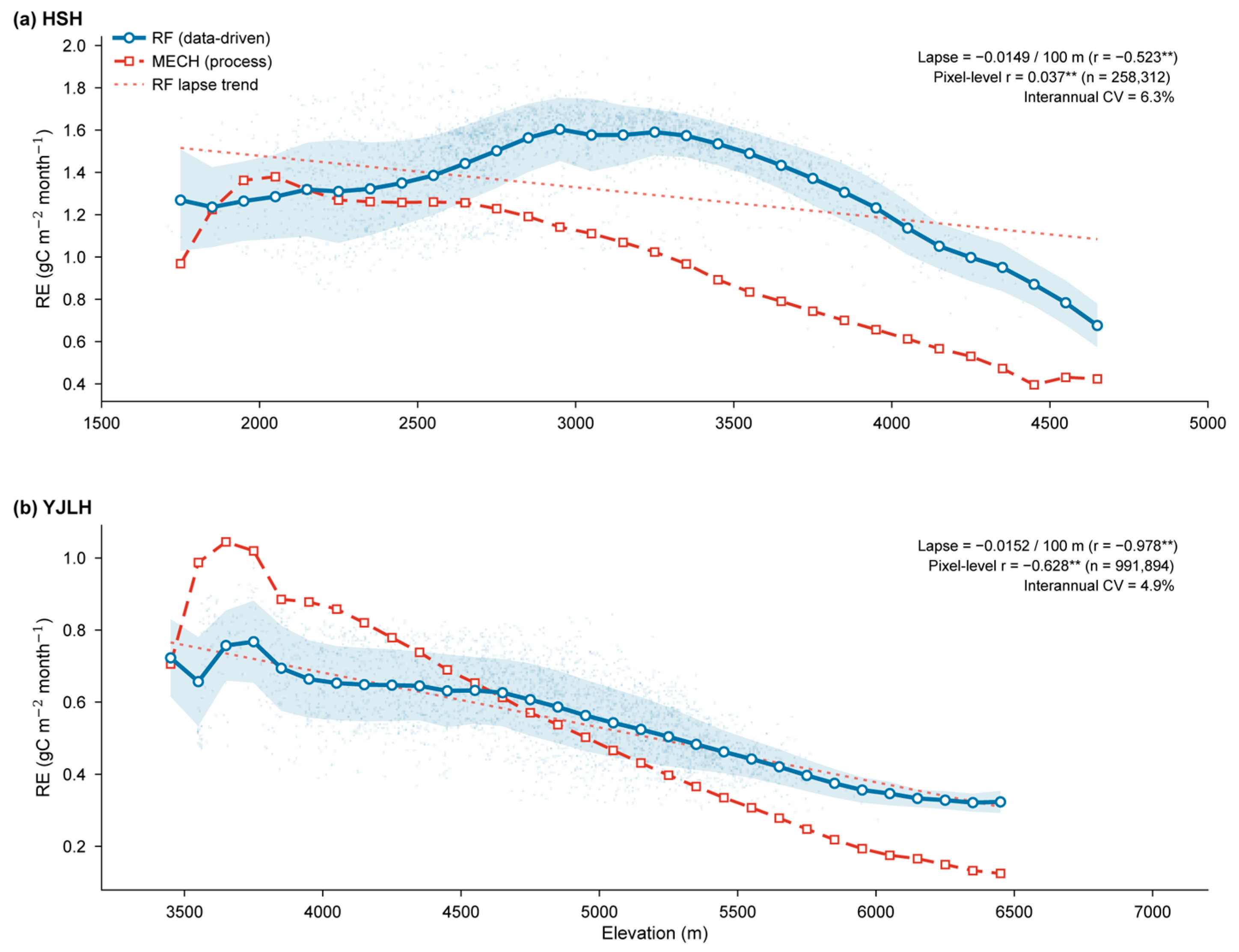
Ecosystem respiration (RE) varied markedly along the elevation gradient (Figure 10), and the nature of this variation differed substantially between the HSH and YJLH. Overall, RE declined with increasing elevation in both basins, but the magnitude of change and the interannual response patterns were inconsistent across elevation zones.

Along the multi-year mean elevation gradient (Figure 10a), RE in the HSH remained high at low-to-mid elevations, peaked at approximately 2800–3300 m, and then declined progressively with further elevation rise. The random forest (RF) model yielded an elevation lapse rate of −0.0149 gC m⁻² month⁻¹ per 100 m, with RE showing a significant negative correlation with elevation (r = −0.523, p < 0.01). The mechanistic model (MECH) produced consistently lower RE values than the RF model across the entire elevation gradient, with a more gradual declining trend. RE was markedly reduced at high elevations (>4200 m), indicating persistent temperature limitation on ecosystem respiration.

The YJLH exhibited a stronger elevation dependence (Figure 10b). RE declined continuously with increasing elevation, yielding a lapse rate of −0.0152 gC m⁻² month⁻¹ per 100 m and a correlation coefficient of r = −0.978 (p < 0.01), indicating that elevation exerts a considerably stronger control on RE in this basin than in the HSH. Compared with the HSH, the YJLH showed lower overall RE levels and a broader spatial extent of low values at high elevations. Above 5500 m in particular, RE remained persistently low, reflecting the pronounced thermal constraint on ecosystem respiration under extreme high-altitude conditions.

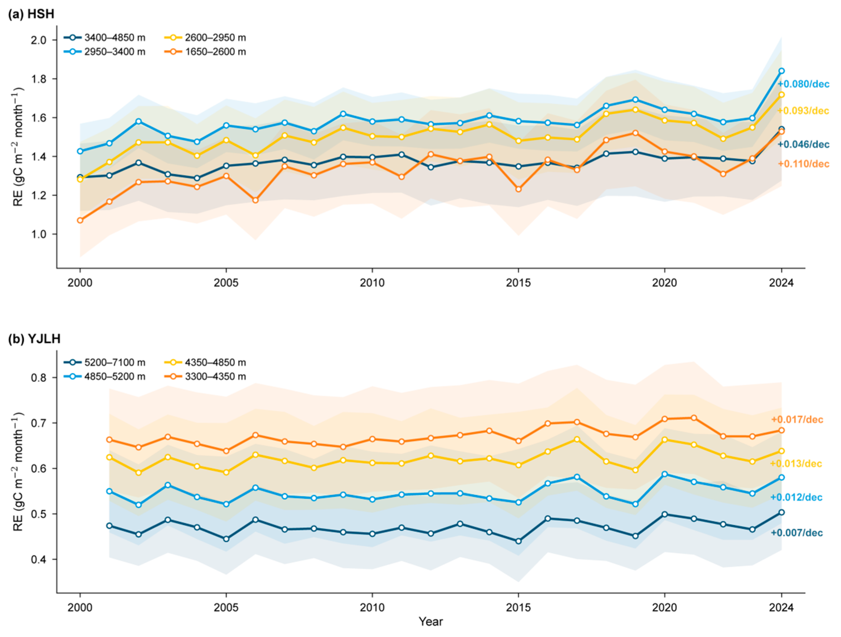
Interannual variation across elevation zones further revealed elevation-dependent responses of RE to environmental change (Figure 11). In the HSH, RE exhibited an increasing trend across all elevation zones. The largest increase occurred in the low-elevation zone (1650–2600 m), with a rate of +0.110 per decade; the increase was comparatively weaker in the mid-to-high elevation zones, reaching only +0.046 per decade in the 3400–4850 m band. Overall, the low-elevation zone combined a higher absolute RE level with a more pronounced long-term increasing trend.

By contrast, the magnitude of RE change across elevation zones in the YJLH was generally smaller. The highest increase occurred in the 3300–4350 m zone (+0.017 per decade), while the high-elevation zone (5200–7100 m) showed only a weak increase (+0.007 per decade). Although all elevation zones exhibited an upward trend, the overall magnitude of increase was markedly lower than that observed in the HSH, suggesting that the RE response to climate change in high-altitude cold regions is comparatively subdued.

Taken together, RE in both basins displayed a pronounced elevation gradient: low-elevation areas generally supported higher ecosystem respiration, whereas RE was substantially reduced in high-altitude cold regions. Concurrently, the long-term trajectories of RE differed appreciably across elevation zones, with low-elevation zones responding more strongly to environmental change and high-elevation zones showing more muted trends overall.

3.6. Q₁₀ Temperature Sensitivity of RE

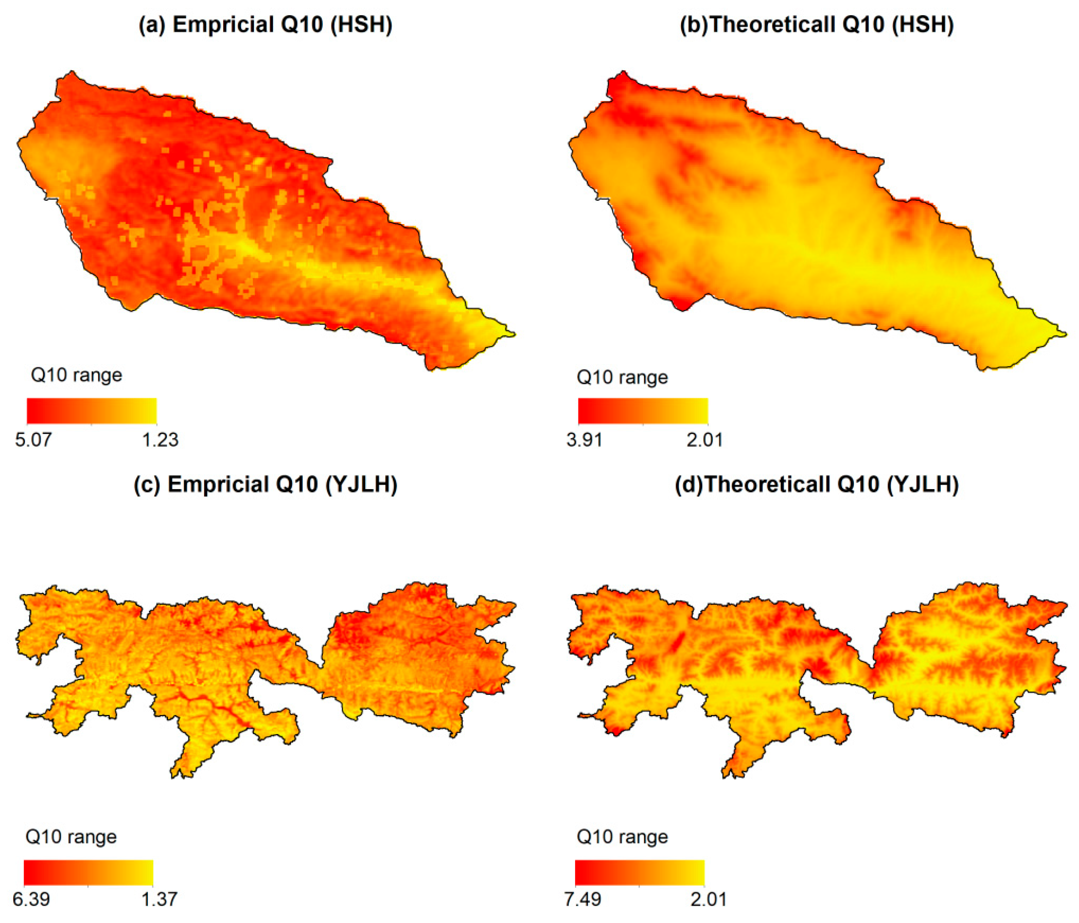
The temperature sensitivity of ecosystem respiration (RE) exhibited pronounced spatial heterogeneity in both basins (Figure 12), and a systematic deviation was evident between the empirical Q₁₀ and the theoretical Q₁₀. Overall, the empirical Q₁₀ derived from the RF model was consistently higher than the theoretical Q₁₀ calculated from the Lloyd–Taylor equation, indicating that the machine-learning model simulates a stronger RE response to temperature change.

In the HSH, the theoretical Q₁₀ averaged 2.48 ± 0.32 (range: 2.01–3.91), whereas the empirical Q₁₀ averaged 3.44 ± 0.66 (range: 1.23–5.05) (

Table 6. Q₁₀ temperature sensitivity statistics.

Watershed	Q10 Statistic	Theory Q10	Experience Q10
HSH	Mean Value	2.482	3.433
	Standard Deviation	0.321	0.670
	Range	[2.01, 3.91]	[1.23, 5.07]
	Q10/1000 m increasing rate	≈0.5
	High-altitude area (mean + 1SD) Q10	≈3.5
	Low-altitude area (mean − 1SD) Q10	≈2.3
YJLH	Mean Value	2.654	3.252
	Standard Deviation	0.384	0.643
	Range	[2.01, 7.49]	[1.37, 6.39]
	Q10/1000 m increasing rate	≈0.8
	High-altitude area (mean + 1SD) Q10	≈5.5
	Low-altitude area (mean − 1SD) Q10	≈2.5

). Spatially, higher Q₁₀ values were located predominantly in the northern and high-altitude areas, while the valley bottoms and low-elevation zones exhibited comparatively lower values.

The YJLH displayed higher and more spatially continuous temperature sensitivity overall. The theoretical Q₁₀ averaged 2.65 ± 0.38 (range: 2.01–7.49) and the empirical Q₁₀ averaged 3.23 ± 0.64 (range: 1.37–6.34). High-value zones were concentrated mainly in the alpine mountains and ridge areas, while the valley bottoms and low-elevation zones maintained lower levels. Compared with the HSH, the YJLH showed a more extensive spatial coverage of high-Q₁₀ areas, suggesting that RE is more sensitive to temperature change under extreme alpine conditions.

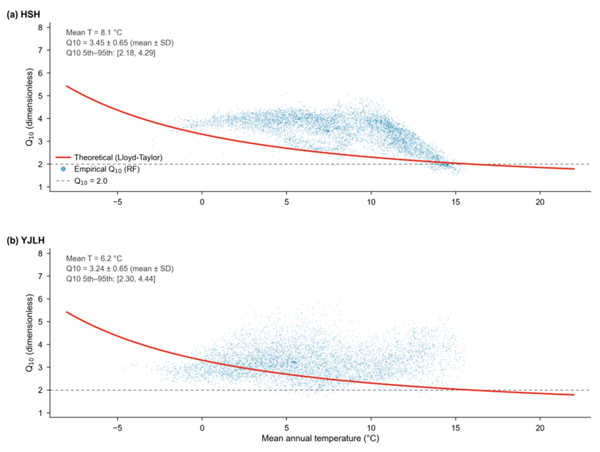
Both the theoretical and empirical Q₁₀ exhibited a pronounced negative correlation with mean annual temperature across both basins (Figure 13). As temperature increased, the theoretical Q₁₀ declined steadily and gradually approached the canonical empirical value of 2.0. The empirical Q₁₀ likewise displayed a declining trend, albeit with greater dispersion. In the HSH (mean annual temperature: 8.1 °C), the empirical Q₁₀ averaged 3.43 ± 0.67; in the YJLH (mean annual temperature: 6.2 °C), it averaged 3.25 ± 0.64. Low-temperature zones consistently corresponded to higher Q₁₀ values, indicating that RE is more sensitive to temperature change in cold environments.

This study conducted a systematic analysis of the variability characteristics of the Q₁₀ scatter. The results showed that, within 2 °C temperature bins, empirical Q₁₀ values varied markedly across different sites. The coefficient of variation (CV) was 0.31 in the HSH and 0.47 in the YJLH, indicating a higher degree of spatial dispersion in temperature sensitivity across the YJLH. Variance decomposition further revealed that temperature alone explained 62% and 41% of the Q₁₀ variance in the HSH and YJLH, respectively, pointing to a dominant but basin-dependent role of temperature in controlling Q₁₀ variability. Incorporating soil moisture and EVI markedly improved model explanatory power, raising the explained variance to 78% (HSH) and 67% (YJLH). These results indicate that water availability and vegetation type play important modulating roles in the temperature response of Q₁₀, and that they partially weaken the explanatory capacity observed under temperature alone. The three factors thus jointly drive the spatial heterogeneity of Q₁₀.

Along the elevation gradient, Q₁₀ showed an overall increasing trend in both basins. In the HSH, Q₁₀ increased by approximately 0.5 per 1000 m rise in elevation, whereas the YJLH exhibited a steeper increase of approximately 0.8 per 1000 m. At high elevations (mean + 1 SD), Q₁₀ reached approximately 3.5 in the HSH and 5.5 in the YJLH; at low elevations (mean − 1 SD), the corresponding values were approximately 2.3 and 2.5, respectively. Taken together, Q₁₀ in both basins displayed pronounced temperature dependence, with higher temperature sensitivity concentrated in high-elevation, low-temperature areas. This pattern suggests that low-temperature limitation may amplify the response of ecosystem respiration to climate warming across the alpine ecosystems of the Qinghai–Tibet Plateau.

4. Discussion

4.1. Predictive Performance of the Random Forest Model and Inter-Basin Differences

The RF model achieved strong RE prediction in both basins, but performance differed substantially. The higher CV R² in the HSH (0.887) compared with the YJLH (0.613) may reflect differences in spatial heterogeneity, data quality, and predictor structure. The YJLH spans approximately 4.7 times the area of the HSH, with an elevation range of nearly 4000 m encompassing ecosystems from alpine steppe to extreme alpine desert. The expanded environmental gradients and topographic complexity produce stronger nonlinearity in RE–environment relationships, increasing modeling difficulty. Prior studies have documented declining machine-learning model performance in large, high-heterogeneity regions [31,32].

Data quality and sample representativeness may also contribute. At elevations above 5500 m in the YJLH, vegetation cover is sparse and RE is low; remote sensing signals are susceptible to mixed-pixel effects from snow, ice, and bare ground, elevating predictor noise. The TPDC RECO product has relatively limited observational sites in extreme high-altitude zones, potentially reducing model generalization at the highest elevations. The uneven spatial distribution of eddy covariance towers on the QTP, with a scarcity of extreme high-altitude stations, has been noted in multiple studies [52,53].

SHAP analysis further demonstrated divergent RE driver structures. In the HSH, RE was controlled primarily by GPP (25.8%) and EVI (14.6%), whereas in the YJLH, precipitation contributed more strongly (18.8%) alongside GPP (26.4%). The more complex driver structure in the YJLH—jointly influenced by vegetation productivity, hydrothermal conditions, and alpine environmental constraints—increases model learning difficulty, consistent with recognized complexity in carbon flux controls in alpine arid regions [22,54]. Despite the lower CV R² in the YJLH, model performance remained within an acceptable range given the strong spatial heterogeneity: machine learning upscaling studies in alpine regions typically report R² of 0.5–0.8 [31,32,33], and the present results fall within this range.

4.2. Spatial Heterogeneity of RE Drivers

This study further refined and supplemented the interpretation of variable importance derived from the SHAP analysis, in order to address potential concerns regarding multicollinearity and attribution bias in model explanation. We emphasize explicitly that SHAP provides marginal decomposition of predictive contributions, rather than direct proof of independent causal pathways. Consequently, interpreting the role of individual variables requires simultaneous consideration of their correlational structure and the underlying mechanisms through which they jointly regulate ecosystem respiration (RE). On this basis, a more circumspect and structured discussion of the roles of different environmental factors in the two basins is presented below.

The SHAP analysis revealed the predictive importance of different environmental variables for RE and the spatial variation in their contributions. Overall, GPP emerged as the most important predictor in both basins (HSH: 25.78%; YJLH: 26.37%), indicating that vegetation productivity carries the highest explanatory weight in RE simulation. However, we further found that RE is not governed by any single factor; rather, it reflects the combined action of several key variables, with precipitation (0.18), air temperature (0.15), EVI (0.12), and soil moisture (0.09) all exhibiting non-negligible contributions. This finding indicates that variation in ecosystem respiration is fundamentally an integrated response to multi-factor coupling.

From a mechanistic perspective, the relationship between GPP and RE reflects the coupled nature of carbon cycling: autotrophic and heterotrophic respiration are jointly constrained by photosynthetic productivity, while GPP simultaneously supplies substrates to soil microorganisms through litter input and root exudates [3,55]. The cumulative contribution of vegetation indices (EVI and NDVI) approached 20%, further indicating that aboveground biomass and canopy structure exert important regulatory effects on RE, consistent with observations from alpine meadows on the Qinghai–Tibet Plateau [29].

It should be noted that a pronounced correlational structure exists among the predictor variables, which may influence the SHAP importance allocation. For example, GPP and EVI showed a strong correlation (r = 0.78), while temperature and elevation were significantly negatively correlated (r = −0.85). Such collinearity among variables means that the importance ranking reflected by SHAP captures not only independent contributions but also the allocation of shared information [56]. Accordingly, the relatively high importance of GPP may, to some degree, also reflect its capacity as an integrative proxy for vegetation state and environmental conditions.

Precipitation exhibited a high contribution in both basins, but its importance was more pronounced in the YJLH (18.81% vs. 12.03%). This difference is closely linked to the contrasting moisture regimes of the two basins. Mean annual precipitation in the HSH is approximately 300–500 mm, whereas in the YJLH it is only 200–400 mm—closer to the moisture limitation threshold for alpine vegetation growth—so water availability exerts a stronger constraint on RE. Previous studies have established that moisture limitation is an important control on RE variation in arid and semi-arid ecosystems [57,58]. Warming experiments on the Qinghai–Tibet Plateau have further demonstrated that the effect of warming on carbon use efficiency depends significantly on soil moisture conditions [59], indicating that hydrothermal coupling is a key regulatory mechanism governing carbon processes in alpine ecosystems.

The direct SHAP contributions of temperature were similar between the two basins (HSH: 10.98%; YJLH: 11.07%), but its ecological role may be partially underestimated. Temperature not only directly affects microbial metabolism and heterotrophic respiration rates, but also indirectly influences RE through its regulation of vegetation productivity. The temperature-response model proposed by Lloyd and Taylor (1994) has been widely used to describe the exponential temperature dependence of soil respiration [35], and subsequent studies have further confirmed that soil temperature is an important factor controlling the seasonal dynamics of RE in alpine ecosystems [27,36,60]. In addition, the sine and cosine variables representing month of the year together contributed approximately 13%, indicating that RE retains a pronounced seasonal cyclicity and reflecting the important regulatory role of phenological processes in ecosystem respiration.

By comparison, the direct SHAP contributions of elevation and soil moisture were low (each approximately 2%). This does not imply that their ecological roles are minor; rather, it likely reflects the fact that their influence is exerted largely through other variables. For instance, elevation indirectly affects RE through the temperature lapse rate and vegetation distribution, while soil moisture shares strong collinearity with precipitation, vegetation indices, and temperature, thereby reducing its independent marginal contribution. This phenomenon—low direct contribution but high mechanistic importance—is a commonly encountered pattern in machine-learning-based ecological studies [34].

Taken together, the driving mechanisms of RE in both basins are characterized by pronounced spatial heterogeneity and multi-factor coupling. The HSH exhibits a structure in which vegetation productivity serves as the core driver and climatic factors provide synergistic regulation, while the YJLH shows a stronger signature of moisture limitation. The flatter contribution structure observed in the YJLH further suggests that its ecological processes are jointly shaped by the steeper elevation gradient and greater environmental heterogeneity. These results indicate that, in high-altitude valley agricultural areas, the formation mechanisms of RE represent an integrated manifestation of biological processes and hydrothermal conditions acting in concert, rather than the outcome of any single dominant factor.

4.3. Elevational Control on Ecosystem Respiration

RE declined with elevation in both basins. Based on 100 m bin means, both the HSH and YJLH exhibited elevation lapse rates of approximately −0.015 g C·m⁻²·month⁻¹ per 100 m. The stronger RE–elevation correlation in the YJLH (r = −0.978 vs. r = −0.523 in the HSH) suggests that elevation exerts tighter control where the elevation span is larger (~3800 m) and the climatic and vegetation zonation is more complete, so elevation integrates temperature, moisture, and vegetation gradients more effectively. Zhao et al. (2017) documented a similar elevation dependence of soil respiration in the central QTP [60]. We note that the correlation coefficients reported here were derived from 100 m bin-mean regression, which enhances signal-to-noise ratio and thus yields stronger correlations than pixel-level analysis.

A notable feature of the HSH elevation profile was a local RE peak at 2800–3300 m, followed by decline at higher elevations. This “mid-elevation peak” departs from the classic monotonic decline pattern and likely reflects optimal hydrothermal conditions and vegetation productivity at intermediate elevations. Similar non-monotonic elevation–respiration relationships have been reported for alpine grasslands on the QTP and in the Andes [60,61]. Aboveground biomass has been shown to explain 21.5–61.6% of RE seasonal variation [29], supporting the role of vegetation productivity in shaping the RE elevation profile.

Interannual RE changes by elevation band demonstrated elevation-dependent responses: low-elevation zones showed larger increases than high-elevation zones in both basins. This suggests that short growing seasons, low substrate availability, and low-temperature limitation continue to suppress rapid RE responses to warming at the highest elevations, a phenomenon described as “response inertia” in alpine ecosystems [29]. With continued warming and permafrost degradation, however, the stability of high-altitude carbon pools may diminish, elevating future carbon release risk [22].

4.4. Temperature Sensitivity (Q₁₀) and Carbon–Climate Implications

Q₁₀ exhibited pronounced spatial heterogeneity and a clear low-temperature enhancement pattern. Empirical Q₁₀ values (HSH: 3.44 ± 0.66; YJLH: 3.24 ± 0.64) exceeded theoretical values (HSH: 2.48 ± 0.32; YJLH: 2.65 ± 0.38), indicating that the actual RE response to temperature is stronger than predicted from purely thermodynamic control. This divergence likely reflects indirect temperature effects mediated through enhanced GPP, increased carbon substrate supply, and stimulated microbial activity. Mahecha et al. (2010), using global FLUXNET data, demonstrated that the apparent temperature sensitivity of RE is substantially reduced after removing the indirect effects of GPP [62], consistent with the present findings.

Q₁₀ was negatively correlated with mean annual temperature, with colder regions corresponding to higher temperature sensitivity. This pattern accords with Arrhenius kinetics and the carbon quality–temperature hypothesis [37], which posits that soil organic matter decomposition at low temperatures requires higher activation energy and is therefore more temperature-sensitive. The global mean apparent Q₁₀ for soil respiration has been estimated at approximately 1.5 [3], but alpine ecosystems consistently exceed this level [29,60], underscoring the heightened responsiveness of cold environments to warming.

Along the elevation gradient, Q₁₀ increased by ~0.5 per 1000 m in the HSH and ~0.8 per 1000 m in the YJLH. At high elevations (mean + 1 SD), Q₁₀ approached 3.5 in the HSH and 5.5 in the YJLH, compared with ~2.3 and ~2.5 at low elevations. Elevated Q₁₀ in high-altitude zones implies that once temperature limitation is overcome, RE may accelerate rapidly, generating a strong positive carbon–climate feedback. Similar elevation-dependent Q₁₀ patterns have been confirmed in QTP alpine meadow experiments [29,60].

4.5. Limitations and Future Directions

Several limitations should be acknowledged. First, observational data deficiency in high-altitude zones remains an important constraint on model accuracy. The current TPDC RECO product and eddy covariance observation network are concentrated at low-to-mid elevations, and long-term measurements above 5500 m remain scarce. Although the QTP flux observation network (TPE) has expanded in recent years [52], sample insufficiency in extreme alpine environments persists, potentially limiting RF model generalization and increasing RE estimation uncertainty at the highest elevations. Long-term continuous observations in extreme high-altitude zones are needed to improve model constraint on carbon flux processes in these environments.

Second, the monthly scale analysis cannot capture rapid RE responses to short-term environmental fluctuations. Under global warming, drought pulses, freeze–thaw cycles, and extreme precipitation events may produce substantial nonlinear effects on alpine ecosystems [63]. Monthly analysis smooths these high-frequency signals to some extent. Future work could incorporate FLUXNET half-hourly observations and high-temporal-resolution remote sensing data to reveal dynamic RE responses to extreme climate events.

Third, disturbance processes such as grazing, land-use change, and permafrost degradation were not incorporated into the modeling framework, despite their potentially profound influence on alpine carbon cycling. Grazing effects on soil respiration in QTP alpine grasslands vary among ecosystem types [64,65], and ongoing permafrost degradation may promote deep organic carbon exposure and enhance heterotrophic respiration [23]. Future work should address the coupling between anthropogenic activities and climate change, particularly whether agricultural management, grazing disturbance, and permafrost degradation jointly amplify carbon release risk in alpine regions.

Fourth, the 1 km spatial resolution adopted here can characterize basin-scale RE patterns but has limited capacity to resolve micro-topographic, slope-aspect, and vegetation-patch effects. Higher-resolution data (e.g., Landsat and Sentinel-2) can more effectively capture landscape-scale carbon flux heterogeneity [32]. Integrating such data with the present framework could improve the spatial expressiveness of carbon cycle studies in alpine mountain regions.

In summary, RE in QTP valley agricultural systems is influenced not only by climate change but also by anthropogenic activities and land-surface processes. Future research that integrates long-term observations, multi-scale remote sensing, and process-based models will be essential for elucidating the mechanisms of alpine agricultural carbon cycle change under continued warming and the associated carbon–climate feedback potential.

5. Conclusions

This study employed a dual-model framework combining a random forest (RF) model with the Lloyd–Taylor mechanistic model to investigate the dynamics of ecosystem respiration (RE) in two representative valley agricultural basins on the Qinghai–Tibet Plateau. By integrating multi-source remote sensing and reanalysis data, we quantified the spatiotemporal patterns, driving mechanisms, and temperature sensitivity of RE over the period 2000–2024.

Overall, RE exhibited a consistent increasing trend in both basins, although with pronounced regional divergence. The random forest model outperformed the mechanistic model in capturing spatial heterogeneity, particularly in the structurally more complex high-altitude YJLH, underscoring the value of data-driven approaches in alpine environments with strong structural heterogeneity.

Gross primary productivity (GPP) emerged as the primary control on RE in both basins, followed by precipitation and vegetation indices, indicating that carbon substrate supply and hydrothermal conditions jointly regulate ecosystem respiration. However, the relative importance of climatic constraints—particularly temperature and precipitation—was greater in the higher-elevation YJLH, reflecting intensified environmental limitation under extreme alpine conditions.

Elevation played a foundational role in shaping RE patterns. RE declined consistently with increasing elevation, while temperature sensitivity (Q₁₀) was enhanced in high-altitude zones. Both the empirical and theoretical Q₁₀ increased along the elevation gradient, with higher values observed in the YJLH, suggesting that cold environments harbour greater potential for carbon release under future warming scenarios.

Spatial analysis further revealed strong and persistent spatial clustering of RE in both basins, with high-value clusters concentrated in low-elevation agricultural valley areas. Land-use patterns reinforced these spatial structures, with cropland and grassland contributing disproportionately to regional carbon fluxes.

Taken together, these findings demonstrate that valley agricultural ecosystems on the Qinghai–Tibet Plateau exhibit pronounced spatial heterogeneity and marked elevation-dependent carbon–climate sensitivity. High-altitude zones are particularly vulnerable to enhanced ecosystem respiration under future warming, a pattern that may amplify regional carbon–climate feedbacks under ongoing climate change.

References

1. Friedlingstein, P.; O’sullivan, M.; Jones, M.W.; Andrew, R.M.; Bakker, D.C.; Hauck, J.; Landschützer, P.; Quéré, C.L.; Luijkx, I.T.; Peters, G.P.; et al. Global carbon budget. Earth Syst. Sci. Data 2023, 15, 5301–5369. [Google Scholar] [CrossRef] [Scilit]
2. Zhu, X.J.; Yu, G.R.; Wang, Q.F.; Gao, Y.N.; Zhao, X.Q.; Han, S.J.; Yan, J.H. The interaction between components of ecosystem respiration in typical forest and grassland ecosystems. Acta Ecol. Sin. 2013, 33, 6925–6934. [Google Scholar] [CrossRef] [Scilit]
3. Bond-Lamberty, B.; Thomson, A. Temperature-associated increases in the global soil respiration record. Nature 2010, 464, 579–582. [Google Scholar] [CrossRef] [Scilit] [PubMed]
4. Bond-Lamberty, B.; Ballantyne, A.; Berryman, E.; Fluet-Chouinard, E.; Jian, J.; Morris, K.A.; Rey, A.; Vargas, R. Twenty years of progress, challenges, and opportunities in measuring and understanding soil respiration. J. Geophys. Res. Biogeosci. 2024, 129, e2023JG007637. [Google Scholar] [CrossRef] [Scilit]
5. Jian, J.; Vargas, R.; Anderson-Teixeira, K.; Stell, E.; Herrmann, V.; Horn, M.; Kholod, N.; Manzon, J.; Marchesi, R.; Paredes, D.; et al. A restructured and updated global soil respiration database (SRDB-V5). Earth Syst. Sci. Data 2021, 13, 255–267. [Google Scholar] [CrossRef] [Scilit]
6. IPCC. Climate Change 2021: The Physical Science Basis. Contribution of Working Group I to the Sixth Assessment Report of the Intergovernmental Panel on Climate Change; Cambridge University Press: Cambridge, UK, 2021. [Google Scholar] [CrossRef] [Scilit]
7. Crippa, M.; Solazzo, E.; Guizzardi, D.; Monforti-Ferrario, F.; Tubiello, F.N.; Leip, A. Food systems are responsible for a third of global anthropogenic GHG emissions. Nat. Food 2021, 2, 198–209. [Google Scholar] [CrossRef] [Scilit] [PubMed]
8. Gao, H.; Tian, H.; Zhang, Z.; Xia, X. Warming-induced greenhouse gas fluxes from global croplands modified by agricultural practices: A meta-analysis. Sci. Total Environ. 2022, 820, 153288. [Google Scholar] [CrossRef] [Scilit] [PubMed]
9. Zhang, Y.; Zou, J.; Dang, S.; Osborne, B.; Ren, Y.; Ju, X. Topography modifies the effect of land-use change on soil respiration: A meta-analysis. Ecosphere 2021, 12, e03845. [Google Scholar]
10. Dong, J.; Sun, S.; Zhan, G.; Sun, J.; Tang, Y.; Wang, Y. Integrated response of crop yields and greenhouse gas emissions to cropland management practices and natural factors: A global meta-analysis. Environ. Res. Lett. 2025, 20, 013007. [Google Scholar] [CrossRef] [Scilit]
11. Zhang, Q.; Wu, J.; Yang, F.; Lei, Y.; Zhang, Q.; Cheng, X. Alterations in soil microbial community composition and biomass following agricultural land use change. Sci. Rep. 2016, 6, 36587. [Google Scholar] [CrossRef] [Scilit] [PubMed]
12. Zhao, Y.L.; Goldberg, S.D.; Xu, J.C.; Harrison, R.D. Spatial and seasonal variation in soil respiration along a slope in a rubber plantation and a natural forest in Xishuangbanna, Southwest China. J. Mt. Sci. 2018, 15, 695–707. [Google Scholar] [CrossRef] [Scilit]
13. Peri, P.L.; Bahamonde, H.; Christiansen, R. Soil respiration in Patagonian semiarid grasslands under contrasting environmental and use conditions. J. Arid Environ. 2015, 119, 1–8. [Google Scholar] [CrossRef] [Scilit]
14. Chen, H.; Zhu, Q.; Peng, C.; Wu, N.; Wang, Y.; Fang, X.; Wu, J. The impacts of climate change and human activities on biogeochemical cycles on the Qinghai-Tibetan Plateau. Glob. Change Biol. 2013, 19, 2940–2955. [Google Scholar]
15. Piao, S.; Wang, X.; Park, T.; Chen, C.; Lian, X.; He, Y.; Bjerke, J.W.; Chen, A.; Ciais, P.; Tømmervik, H.; et al. Characteristics, drivers and feedbacks of global greening. Nat. Rev. Earth Environ. 2020, 1, 14–27. [Google Scholar]
16. Yao, T.; Xue, Y.; Chen, D.; Chen, F.; Thompson, L.; Cui, P.; Koike, T.; Lau, W.K.-M.; Lettenmaier, D.; Mosbrugger, V.; et al. Recent third pole’s rapid warming accompanies cryospheric melt and water cycle intensification and interactions between monsoon and environment: Multidisciplinary approach with observations, modeling, and analysis. Bull. Am. Meteorol. Soc. 2019, 100, 423–444. [Google Scholar] [CrossRef] [Scilit]
17. You, Q.; Chen, D.; Wu, F.; Pepin, N.; Cai, Z.; Ahrens, B.; Jiang, Z.; Wu, Z.; Kang, S.; AghaKouchak, A. Elevation dependent warming over the Tibetan Plateau: Patterns, mechanisms and perspectives. Earth-Sci. Rev. 2020, 210, 103349. [Google Scholar] [CrossRef] [Scilit]
18. Kuang, X.; Jiao, J.J. Review on climate change on the Tibetan Plateau during the last half century. J. Geophys. Res. Atmos. 2016, 121, 3979–4007. [Google Scholar] [CrossRef] [Scilit]
19. Wei, D.; Qi, Y.; Ma, Y.; Wang, X.; Ma, W.; Gao, T.; Huang, L.; Zhao, H.; Zhang, J.; Wang, X. Plant uptake of CO2 outpaces losses from permafrost and plant respiration on the Tibetan Plateau. Proc. Natl. Acad. Sci. USA 2021, 118, e2015283118. [Google Scholar] [PubMed]
20. Ma, W.; Wu, T.; Wu, X.; Yang, S.; Li, R.; Zhou, S.; Li, X.; Zhu, X.; Hao, J.; Ni, J.; et al. Carbon budgets and environmental controls in alpine ecosystems on the Qinghai-Tibet Plateau. Catena 2023, 229, 107224. [Google Scholar] [CrossRef] [Scilit]
21. Shen, T.; Yu, Z.; Ju, Q.; Jin, J.; Wang, G.; Liu, Y.; Hu, C.; Lyu, S.; Lin, H.; Si, X.; et al. Climate change intensifies carbon emissions from the Earth’s Third Pole: Projected trajectories of soil and ecosystem respiration. Glob. Planet. Change 2026, 259, 105359. [Google Scholar]
22. Liu, L.; Zhuang, Q.; Zhao, D.; Zheng, D.; Kou, D.; Yang, Y. Permafrost degradation diminishes terrestrial ecosystem carbon sequestration capacity on the Qinghai-Tibetan plateau. Glob. Biogeochem. Cycles 2022, 36, e2021GB007068. [Google Scholar]
23. Duncan, B.; McKay, R.; Levy, R.; Naish, T.; Prebble, J.G.; Sangiorgi, F.; Krishnan, S.; Hoem, F.; Clowes, C.; Jones, T.D.; et al. Climatic and tectonic drivers of late Oligocene Antarctic ice volume. Nat. Geosci. 2022, 15, 819–825. [Google Scholar] [CrossRef] [Scilit]
24. Du, X.; Li, Q.; Zhao, L.; Shen, Y.; Zhang, S.; Zhang, Y.; Wang, H.; Xu, J. Identification of cropland in Tibetan Plateau based on time series remote sensing features. Geocarto Int. 2024, 39, 2375583. [Google Scholar] [CrossRef] [Scilit]
25. Yu, L.; Liu, S.; Wang, F.; Liu, Y.; Liu, H.; Wang, Q.; Tran, L.-S.P.; Dong, Y.; Li, W. Strategies for agricultural production management based on land, water and carbon footprints on the Qinghai-Tibet Plateau. J. Clean. Prod. 2022, 362, 132563. [Google Scholar] [CrossRef] [Scilit]
26. Liu, Y.; Wang, X.; Xin, L.; Lu, Y. Impact of farmland change on vegetation NPP in the one river and two streams region of Tibet. Land 2022, 11, 2223. [Google Scholar] [CrossRef] [Scilit]
27. Kato, T.; Tang, Y.; Gu, S.; Hirota, M.; Cui, X.; Du, M.; Li, Y.; Zhao, X.; Oikawa, T. Seasonal patterns of gross primary production and ecosystem respiration in an alpine meadow ecosystem on the Qinghai-Tibetan Plateau. J. Geophys. Res. Atmos. 2004, 109, D12109. [Google Scholar]
28. Xu, D.; Mou, W.; Wang, X.; Zhang, R.; Gao, T.; Ai, D.; Yuan, J.; Zhang, R.; Fang, X. Consistent responses of ecosystem CO2 exchange to grassland degradation in alpine meadow of the Qinghai-Tibetan Plateau. Ecol. Indic. 2022, 141, 109036. [Google Scholar] [CrossRef] [Scilit]
29. Hu, Y.; Jiang, L.; Wang, S.; Zhang, Z.; Luo, C.; Bao, X.; Niu, H.; Xu, G.; Duan, J.; Zhu, X.; et al. The temperature sensitivity of ecosystem respiration to climate change in an alpine meadow on the Tibet plateau: A reciprocal translocation experiment. Agric. For. Meteorol. 2016, 216, 93–104. [Google Scholar] [CrossRef] [Scilit]
30. Liu, Z.; Deng, Z.; He, G.; Wang, H.; Zhang, X.; Lin, J.; Qi, Y.; Liang, X. Challenges and opportunities for carbon neutrality in China. Nat. Rev. Earth Environ. 2022, 3, 141–155. [Google Scholar]
31. Jung, M.; Schwalm, C.; Migliavacca, M.; Walther, S.; Camps-Valls, G.; Koirala, S.; Anthoni, P.; Besnard, S.; Bodesheim, P.; Carvalhais, N.; et al. Scaling carbon fluxes from eddy covariance sites to globe: Synthesis and evaluation of the FLUXCOM approach. Biogeosciences 2020, 17, 1343–1365. [Google Scholar] [CrossRef] [Scilit]
32. Tramontana, G.; Jung, M.; Schwalm, C.R.; Ichii, K.; Camps-Valls, G.; Ráduly, B.; Reichstein, M.; Arain, M.A.; Cescatti, A.; Kiely, G.; et al. Predicting carbon dioxide and energy fluxes across global FLUXNET sites with regression algorithms. Biogeosciences 2016, 13, 4291–4313. [Google Scholar] [CrossRef] [Scilit]
33. Zeng, J.; Matsunaga, T.; Tan, Z.H.; Saigusa, N.; Shirai, T.; Tang, Y.; Peng, S.; Fukuda, Y. Global terrestrial carbon fluxes of 1999–2019 estimated by upscaling eddy covariance data with a random forest. Sci. Data 2020, 7, 313. [Google Scholar] [CrossRef] [Scilit] [PubMed]
34. Lundberg, S.M.; Lee, S.-I. A unified approach to interpreting model predictions. Adv. Neural Inf. Process. Syst. 2017, 30, 4765–4774. [Google Scholar]
35. Lloyd, J.; Taylor, J.A. On the temperature dependence of soil respiration. Funct. Ecol. 1994, 8, 315–323. [Google Scholar] [CrossRef] [Scilit]
36. Reichstein, M.; Falge, E.; Baldocchi, D.; Papale, D.; Aubinet, M.; Berbigier, P.; Bernhofer, C.; Buchmann, N.; Gilmanov, T.; Granier, A.; et al. On the separation of net ecosystem exchange into assimilation and ecosystem respiration: Review and improved algorithm. Glob. Change Biol. 2005, 11, 1424–1439. [Google Scholar] [CrossRef] [Scilit]
37. Davidson, E.A.; Janssens, I.A. Temperature sensitivity of soil carbon decomposition and feedbacks to climate change. Nature 2006, 440, 165–173. [Google Scholar] [CrossRef] [Scilit] [PubMed]
38. Jung, M.; Reichstein, M.; Bondeau, A. Towards global empirical upscaling of FLUXNET eddy covariance observations: Validation of a model tree ensemble approach using a biosphere model. Biogeosciences 2009, 6, 2001–2013. [Google Scholar] [CrossRef] [Scilit]
39. Lieff, N.; Metzen, D.; Ewenz, C.; Isaac, P.; McHugh, I.; Griebel, A. Assessing the optimal drivers for flux data gap-filling using random forest networks. In Proceedings of the EGU General Assembly Conference Abstracts, Vienna, Austria, 27 April–2 May 2025; p. EGU25-9368. [Google Scholar]
40. Ru, J.; Wan, S.; Xia, J.; Niu, S.; Hui, D.; Song, J.; Feng, J.; Sun, D.; Wang, H.; Qiu, X. Advanced precipitation peak offsets middle growing-season drought in impacting grassland C sink. New Phytol. 2024, 244, 1775–1787. [Google Scholar] [PubMed]
41. Gao, Y.; Yu, G.; Li, S.; Yan, H.; Zhu, X.; Wang, Q.; Shi, P.; Zhao, L.; Li, Y.; Zhang, F.; et al. A remote sensing model to estimate ecosystem respiration in Northern China and the Tibetan Plateau. Ecol. Model. 2015, 304, 34–43. [Google Scholar] [CrossRef] [Scilit]
42. Teixeira, M.A.; Salman, T.; Zolanvari, M.; Jain, R.; Meskin, N.; Samaka, M. SCADA system testbed for cybersecurity research using machine learning approach. Future Internet 2018, 10, 76. [Google Scholar] [CrossRef] [Scilit]
43. Dwiyanti, L.; Wibisono, S.R.; Nambo, H. ContextualSHAP: Enhancing SHAP explanations through contextual language generation. In Proceedings of the 2025 7th World Symposium on Software Engineering; Association for Computing Machinery: New York, NY, USA, 2025; pp. 231–237. [Google Scholar]
44. Kamal, N.; Pachauri, S. Mann–Kendall test—A novel approach for statistical trend analysis. Int. J. Comput. Trends Technol. 2018, 63, 18–21. [Google Scholar]
45. El Kasri, J.; Lahmili, A.; Soussi, H.; Jaouda, I.; Bentaher, M. Trend analysis of meteorological variables: Rainfall and temperature. Civ. Eng. J. 2021, 7, 1868–1879. [Google Scholar] [CrossRef] [Scilit]
46. Fu, W.J.; Jiang, P.K.; Zhou, G.M.; Zhao, K.L. Using Moran’s I and GIS to study the spatial pattern of forest litter carbon density in a subtropical region of southeastern China. Biogeosciences 2014, 11, 2401–2409. [Google Scholar]
47. Lei, J.; Chen, Z.; Wu, T.; Li, Y.; Yang, Q.; Chen, X. Spatial autocorrelation pattern analysis of land use and the value of ecosystem services in northeast Hainan Island. Acta Ecol. Sin. 2019, 39, 2366–2377. [Google Scholar] [CrossRef] [Scilit]
48. Shi, Z. Soil respiration and its regulating factor along an elevation gradient in Wuyi Mountain of Southeast China. Chin. J. Ecol. 2008, 27, 562–568. [Google Scholar]
49. Ma, M.; Zang, Z.; Xie, Z.; Chen, Q.; Xu, W.; Zhao, C.; Shen, G. Soil respiration of four forests along elevation gradient in northern subtropical China. Ecol. Evol. 2019, 9, 12846–12857. [Google Scholar] [CrossRef] [Scilit] [PubMed]
50. Wang, W.; Wang, H.; Zu, Y.; Li, X.; Koike, T. Characteristics of the temperature coefficient, Q10, for the respiration of non-photosynthetic organs and soils of forest ecosystems. Front. For. China 2006, 1, 125–135. [Google Scholar] [CrossRef] [Scilit]
51. Jiang, J.; Feng, L.; Hu, J.; Zhu, C.; Li, G.; Chen, T. Quantifying the intrinsic Q10 of ecosystem and component respiration in a eucalypt forest: Implications for climate-carbon feedback. Plant Cell Environ. 2026, 49, 1078–1091. [Google Scholar] [PubMed]
52. Wang, Y.; Xiao, J.; Ma, Y.; Luo, Y.; Hu, Z.; Li, F.; Li, Y.; Gu, L.; Li, Z.; Yuan, L. Carbon fluxes and environmental controls across different alpine grassland types on the Tibetan Plateau. Agric. For. Meteorol. 2021, 311, 108694. [Google Scholar] [CrossRef] [Scilit]
53. Chen, Y.; Yang, K.; He, J.; Qin, J.; Shi, J.; Du, J.; He, Q. Improving land surface temperature modeling for dry land of China. J. Geophys. Res. Atmos. 2011, 116, D20104. [Google Scholar] [CrossRef] [Scilit]
54. Biederman, J.A.; Scott, R.L.; Bell, T.W.; Bowling, D.R.; Dore, S.; Garatuza-Payan, J.; Kolb, T.E.; Krishnan, P.; Krofcheck, D.J.; Litvak, M.E.; et al. CO2 exchange and evapotranspiration across dryland ecosystems of southwestern North America. Glob. Change Biol. 2017, 23, 4204–4221. [Google Scholar] [CrossRef] [Scilit]
55. Janssens, I.A.; Lankreijer, H.; Matteucci, G.; Kowalski, A.S.; Buchmann, N.; Epron, D.; Pilegaard, K.; Kutsch, W.; Longdoz, B.; Grünwald, T.; et al. Productivity overshadows temperature in determining soil and ecosystem respiration across European forests. Glob. Change Biol. 2001, 7, 269–278. [Google Scholar] [CrossRef] [Scilit]
56. Bond-Lamberty, B.; Thomson, A. A global database of soil respiration data. Biogeosciences 2010, 7, 1915–1926. [Google Scholar] [CrossRef] [Scilit]
57. Moyano, F.E.; Manzoni, S.; Chenu, C. Responses of soil heterotrophic respiration to moisture availability: An exploration of processes and models. Soil Biol. Biochem. 2013, 59, 72–85. [Google Scholar] [CrossRef] [Scilit]
58. Wang, T.; Yang, D.; Yang, Y.; Piao, S.; Li, X.; Cheng, G.; Fu, B. Permafrost thawing puts the frozen carbon at risk over the Tibetan Plateau. Sci. Adv. 2020, 6, eaaz3513. [Google Scholar] [CrossRef] [Scilit] [PubMed]
59. Quan, Q.; Ma, F.; Wang, J.; Tian, D.; Zhou, Q.; Niu, S. Contextualized response of carbon-use efficiency to warming at the plant and ecosystem levels. Sci. Total Environ. 2023, 885, 163777. [Google Scholar] [CrossRef] [Scilit] [PubMed]
60. Zhao, J.; Li, R.; Li, X.; Tian, L. Environmental controls on soil respiration in alpine meadow along a large altitudinal gradient on the central Tibetan Plateau. Catena 2017, 159, 84–92. [Google Scholar] [CrossRef] [Scilit]
61. Zimmermann, M.; Meir, P.; Bird, M.I.; Malhi, Y.; Ccahuana, A.J.Q. Climate dependence of heterotrophic soil respiration from a soil-translocation experiment along a 3000 m tropical forest altitudinal gradient. Eur. J. Soil Sci. 2009, 60, 895–906. [Google Scholar]
62. Mahecha, M.D.; Reichstein, M.; Carvalhais, N.; Lasslop, G.; Lange, H.; Seneviratne, S.I.; Vargas, R.; Ammann, C.; Arain, M.A.; Cescatti, A.; et al. Global convergence in the temperature sensitivity of respiration at ecosystem level. Science 2010, 329, 838–840. [Google Scholar] [CrossRef] [Scilit] [PubMed]
63. Reichstein, M.; Bahn, M.; Ciais, P.; Frank, D.; Mahecha, M.D.; Seneviratne, S.I.; Zscheischler, J.; Beer, C.; Buchmann, N.; Frank, D.C.; et al. Climate extremes and the carbon cycle. Nature 2013, 500, 287–295. [Google Scholar] [CrossRef] [Scilit] [PubMed]
64. Mao, Y.; Du, Y.; Chen, K. Grazing increased alpine grassland soil respiration rates on the Tibetan Plateau. Front. Soil Sci. 2025, 4, 1429371. [Google Scholar] [CrossRef] [Scilit]
65. Zhao, J.; Luo, T.; Li, R.; Li, X.; Tian, L. Grazing effect on growing season ecosystem respiration and its temperature sensitivity in alpine grasslands along a large altitudinal gradient on the central Tibetan Plateau. Agric. For. Meteorol. 2016, 218–219, 114–121. [Google Scholar] [CrossRef] [Scilit]
Figure 1. Location of the Huangshui River Basin (HSH) and Yijianglianghe River Basin (YJLH) on the Qinghai–Tibetan Plateau. (a) is the study area map, (b) is the Huangshui River and River Basin (HSH) DEM map, (c) is a river two river basin (YJLH) DEM map.
Agriculture 16 01429 g001
Figure 2. SHAP bee-swarm plots for the (a) Huangshui River Basin and (b) Yijianglianghe River Basin.
Agriculture 16 01429 g002
Figure 3. Dual-model scatter density comparison for (a) the HSH and (b) the YJLH.
Agriculture 16 01429 g003
Figure 4. Interannual RE trends from RF and MECH models for (a) the HSH and (b) the YJLH. Notes: ** is p < 0.01, highly significant; ns is not significant (p > 0.05).
Agriculture 16 01429 g004
Figure 5. Multi-year mean RE spatial distribution: RF, MECH, and difference maps for the HSH (ac) and the YJLH (df).
Agriculture 16 01429 g005
Figure 6. Spatial distribution of RE in the HSH and YJLH across the study period.
Agriculture 16 01429 g006
Figure 7. Mann–Kendall trend test and Sen’s slope of RE for the HSH (ac) and the YJLH (df).
Agriculture 16 01429 g007
Figure 8. Land-use distribution in the HSH and YJLH.
Agriculture 16 01429 g008
Figure 9. Land-use transition matrices for the HSH and YJLH.
Agriculture 16 01429 g009
Figure 10. RE along the elevation gradient for (a) the HSH and (b) the YJLH. Notes: ** is p < 0.01, highly significant; ns is not significant (p > 0.05).
Agriculture 16 01429 g010
Figure 11. RE time series by elevation band for the HSH and YJLH.
Agriculture 16 01429 g011
Figure 12. Q10 temperature dependence.
Agriculture 16 01429 g012
Figure 13. Q10 temperature dependence: theoretical curves and observed scatter for the HSH and YJLH.
Agriculture 16 01429 g013