AHP-Based Ranking of Durum Wheat Management Scenarios in a Mediterranean Environment

Abstract

The analytic hierarchy process (AHP) was applied to six agronomic scenarios for durum wheat (Triticum durum Desf.) in the Capitanata plain (Apulia, southern Italy), combining three sowing dates (15 October, 1 November, and 15 November) with two water regimes (rainfed; supplemental irrigation at flowering). Five performance indicators were derived from AquaCrop-GIS simulations coupled with cradle-to-gate life-cycle assessment: grain yield, CO₂-equivalent emissions (CO₂_eq), carbon footprint (CFP), total water consumption (TotW), and water footprint (WFP). Six theoretical decision profiles were defined through a symmetric weight scheme (w = 0.60 for the dominant criterion, w = 0.10 for each of the remaining four; balanced profile with equal weights). The rankings revealed a systematic inversion between absolute and ratio indicators: under absolute-metric profiles, the lowest-yielding scenario paradoxically ranked first because reduced productivity mechanically lowered per-hectare resource consumption, whereas under ratio-metric and balanced profiles, early-November rainfed sowing consistently led the rankings. Switching point analyses quantified the weight thresholds at which leadership transitions occurred, providing a continuous sensitivity assessment of the dominant weight, and the AHP procedure was also applied to the 72 simulation replicates spanning the soil × climatic-cell variability of the 2013–2023 dataset to obtain empirical rank distributions for each scenario under each profile. The results highlight that the choice between absolute and ratio environmental indicators is a substantive methodological decision that directly affects the ranking of agronomic alternatives in multi-criteria evaluation.

1. Introduction

Durum wheat (Triticum durum Desf.) is the backbone of Mediterranean cereal systems. The Mediterranean basin supplies approximately 60% of global durum wheat production [1], sustaining the entire semolina, pasta, and couscous value chain across a geographical arc that extends from Morocco and Spain through Italy, Greece, and Turkey to the Levant. In Italy, the Capitanata plain of Apulia—one of the flattest and most intensively farmed areas of southern Europe—concentrates about 38% of the national acreage dedicated to this crop [2]. Cultivation is predominantly rainfed, managed as continuous monoculture under conventional tillage, and has remained structurally stable for decades while facing mounting pressure from climate change, evolving environmental regulation and volatility in grain markets.

The Mediterranean climate imposes well-documented constraints on winter cereals. Inter-annual variability of growing-season rainfall is high and seasonally skewed toward autumn and winter, so that late-season water deficits frequently coincide with the critical grain-filling phase of wheat [3,4]. At the same time, the frequency of heat stress events during anthesis and early grain fill has been increasing, and regional projections consistently indicate further warming and reductions in growing-season precipitation by mid-century [3,4]. These dynamics amplify the importance of low-cost management decisions that remain available to farmers, chief among them the sowing date and the use of limited supplemental irrigation.

Sowing date is the single most accessible lever: a 2- to 4-week shift realigns the phenological calendar of the crop with respect to seasonal temperature and rainfall, without any change in inputs, machinery, or genetics. Early-November sowing in Capitanata places heading in late April and physiological maturity in late June, exposing the grain-filling phase to a cooler thermal window and maximising the productive use of spring rains [5,6]. Mid-November sowing delays maturity by approximately 2 weeks, compressing the grain-filling period under increasing heat demand. Simulation-based and empirical analyses consistently report yield advantages of early over late November sowing of the order of 10–15% in southern Italian environments [5]. Supplemental irrigation in Capitanata is characteristically conservative, typically one or two applications at flowering with total volumes not exceeding 60 mm per season, aimed at stabilising yields in anomalously dry years rather than at intensifying production [5].

The evaluation of these management options is inherently multi-objective. A scenario that maximises yield may simultaneously increase per-hectare water use and absolute greenhouse gas (GHG) emissions; conversely, minimising total water consumption may come at the cost of lower productivity and hence a higher water footprint per unit of product. The tension is especially acute when comparing absolute indicators—total CO₂-equivalent emissions per hectare (CO₂_eq) and total water consumption per hectare (TotW)—with ratio indicators—carbon footprint per kilogram of grain (CFP) and water footprint per kilogram of grain (WFP). The two families of metrics may assign first place to entirely different scenarios and point in opposite directions, a possibility consistent with concerns raised in the life-cycle assessment (LCA) literature on agricultural systems regarding the choice of functional unit [7,8] and tested empirically in the present analysis. Making this trade-off explicit, transparent, and quantifiable has direct implications for how environmental performance standards are framed and how incentive mechanisms under the Common Agricultural Policy (CAP) 2023–2027 are designed [9].

The analytic hierarchy process (AHP), introduced by Saaty [10], provides a well-established multi-criteria decision analysis (MCDA) method for ranking alternatives under multiple, potentially conflicting criteria. Its principal strength is the explicit formalisation of criterion weights, which makes stakeholder priorities transparent and allows the sensitivity of rankings to weight changes to be systematically examined through switching point and robustness analyses. AHP has been applied across a broad range of agricultural contexts, including criterion prioritisation in crop model design [11], land consolidation [12], land suitability assessment in arid regions [13], and durum wheat land suitability [14]. Eco-efficiency analyses of Mediterranean durum wheat under different water and nitrogen inputs have been pursued through life-cycle methods [15], yet without applying MCDA to rank alternative management scenarios. The application of AHP to the systematic comparison of absolute versus ratio environmental indicators derived from process-based crop simulation models has been the subject of comparatively fewer dedicated investigations in the agricultural MCDA literature, and applications combining switching point analysis with pairwise AHP ranking to quantify the weight thresholds at which supplemental irrigation becomes environmentally justified appear to remain limited in the Mediterranean durum wheat literature. Several known limitations of AHP—including the dependence of rankings on the chosen weighting scheme, the potential for rank reversal when alternatives are added or removed, and the inconsistency that may arise from subjective pairwise judgements—are explicitly addressed in the present analysis through (i) the systematic exploration of multiple symmetric weight configurations across six decision profiles, (ii) the switching point analysis, and (iii) the analytical construction of perfectly consistent pairwise comparison matrices (CR = 0) from ratio-normalised indicator values.

AquaCrop, the FAO crop water productivity model [16,17], provides a mechanistic basis for evaluating crop responses to pedo-climatic variability and management decisions. Its GIS extension enables spatially distributed scenario analysis over large territories and extended time horizons. Coupled with the Carbon and Water Footprint (CWFP) tool (version 1.0) [18]—a cradle-to-gate LCA application tailored to Mediterranean cereal systems with ECOINVENT v.3 process data—this modelling chain generates multidimensional output datasets that form an ideal empirical foundation for AHP analysis. A recent application to the Capitanata plain [5] produced a six-scenario, five-indicator dataset covering 10 cropping years (2013–2023) across 432 pedo-climatic combinations. That study analysed individual indicator responses and their sensitivity, but did not formalise the multi-indicator trade-offs into a structured, multi-criteria decision support analysis.

The present paper addresses this gap. AHP with a symmetric weight scheme is applied to rank the six agronomic scenarios across six decision profiles, each representing a distinct priority structure. The symmetric design (w = 0.60 to the dominant criterion and w = 0.10 to each of the remaining four) ensures transparency, internal consistency, and comparability across profiles. By explicitly separating CO₂_eq from CFP and TotW from WFP, the analysis directly tests whether the choice between absolute and ratio indicators constitutes a substantive methodological decision with real consequences for management recommendations. Switching point analyses for three criteria quantify the weight thresholds at which leadership changes, providing quantitative and actionable criteria for choosing between management options under any combination of priorities.

2. Materials and Methods

2.1. Study Area and Data Sources

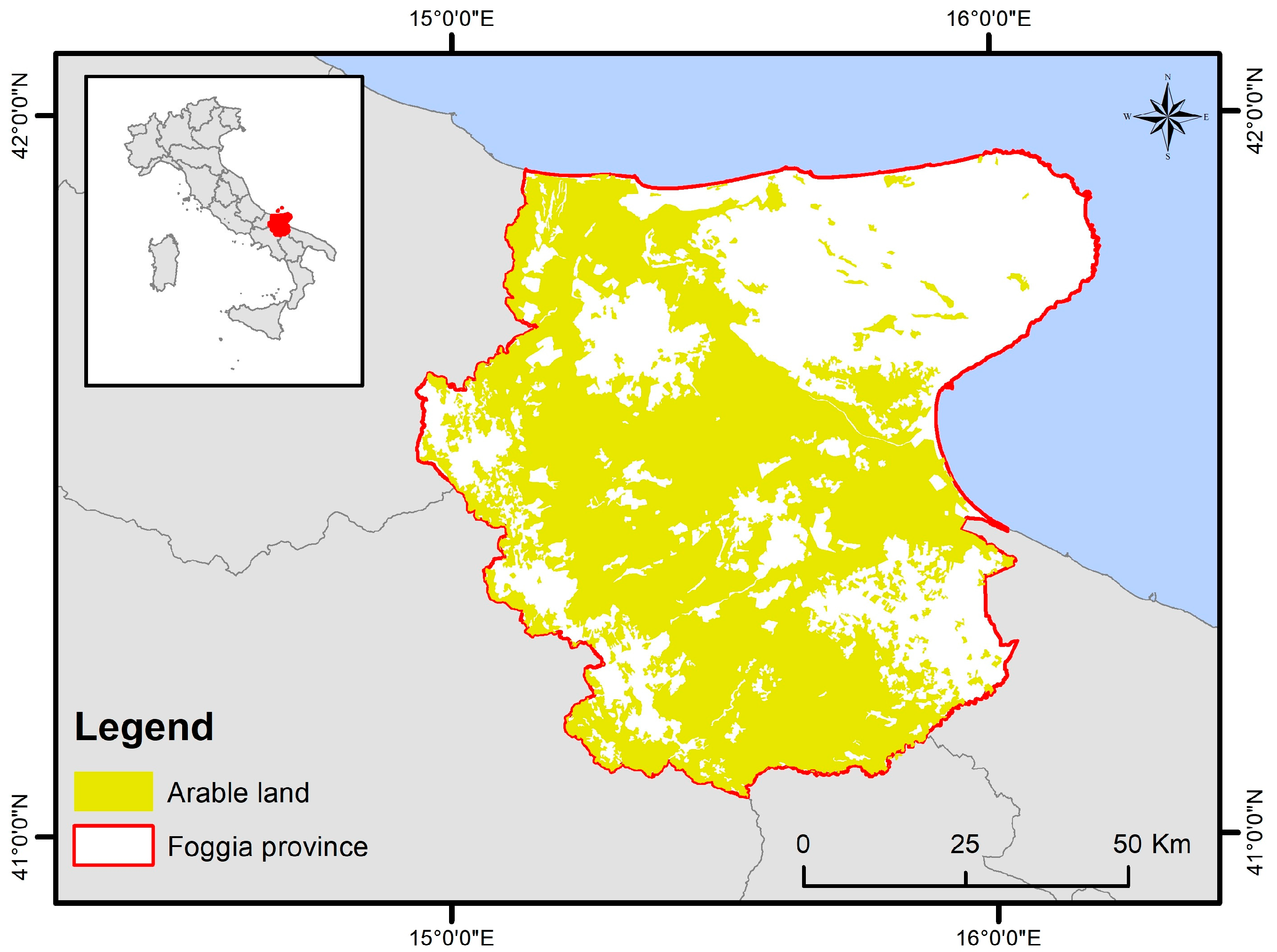
The study area is the Capitanata plain (province of Foggia, Apulia region, southern Italy; centroid approximately 41°27′ N, 15°33′ E, 76 m a.s.l.), Italy’s leading durum wheat production territory (Figure 1). The study area extends approximately 80 km north–south by 100 km east–west, covering about 7000 km² (map projection WGS 84, EPSG:4326), with agricultural land identified from the Regional Land Use Cover database of Apulia [19]. The data underlying the present multi-criteria analysis derive from a process-based modelling exercise covering 10 consecutive cropping years, from 1 January 2013 to 31 December 2023 [5]; daily climatic forcing for the same decade was obtained from the JRC Agri4Cast database [20]. All performance data used in this study were from [5], which reports mean values per agronomic scenario averaged over the 2013–2023 simulation period and across 432 combinations of soil type and climatic cell. Crop simulations used AquaCrop-GIS (v. 2.1) [16,17] with 25 soil profiles from the Harmonised World Soil database [21] and 15 climatic grid cells (25 × 25 km, daily resolution). Crop parameterisation followed the local calibration for winter durum wheat in Capitanata [22]. Environmental indicators were estimated using the CWFP tool [18], implementing a cradle-to-gate LCA boundary following the ILCD 2011 Midpoint methodology with ECOINVENT v.3 process data. No new field data were collected for the present study; the analysis is performed entirely on the simulation outputs published in [5]. The present analysis is, accordingly, complementary to [5], where [5] reports the per-scenario indicator means and the AquaCrop-GIS simulation framework that produced them, the present study layers a multi-criteria evaluation protocol (pairwise AHP ranking, switching point analysis, replicate-based rank distributions, and normalisation-sensitivity diagnostics) on top of that simulation output to address a distinct question—how absolute and ratio environmental indicators jointly shape AHP rankings across distinct decision profiles.

The simulation domain comprised 25 soil profiles and 15 climatic grid cells covering the territory of the Capitanata plain. After spatial intersection of the soil and climate databases, 72 distinct soil × climatic-cell combinations corresponded to agricultural land in the study area and yielded valid AquaCrop-GIS output for all six management scenarios. Each of the six scenarios was simulated on each of these 72 combinations over 10 cropping years (2013–2023), producing 6 × 72 = 432 simulation runs in total. Each “replicate” corresponds to one soil × climatic-cell combination, so the 72 replicates represent the 72 distinct pedo-climatic contexts in which the six scenarios were evaluated. The decadal time series was collapsed to the 10-year mean within each replicate × scenario, so that each replicate provided one 10-year mean performance value per scenario and per indicator. The mean-based AHP analysis aggregated the 72 replicates into a single representative scenario value per indicator (used as input to the pairwise matrices and to Equation (8)); the replicate-based analysis applied the same AHP procedure to each of the 72 replicates separately, generating empirical rank distributions across the full pedo-climatic variability of the territory.

2.2. Scenarios and Performance Indicators

Six agronomic scenarios are defined by the factorial combination of three sowing dates—15 October, 1 November, and 15 November—with two water regimes: rainfed (scenarios S1–S3) and supplemental irrigation at flowering, with a maximum of two events and a total volume not exceeding 60 mm per season (scenarios S4–S6). The actual seasonal irrigation volumes vary across the three irrigated scenarios (13, 28, and 41 mm for S4, S5, and S6, respectively) because AquaCrop-GIS [5,16,17] triggers supplemental water in response to the soil-water deficit accumulated at flowering, and later sowing exposes the crop to lower mid-season rainfall and to earlier soil-water depletion at this critical phenological window. The 60 mm seasonal cap is therefore never reached in this dataset. Five performance indicators are considered: grain yield (Yield, kg ha⁻¹), total CO₂-equivalent emissions per hectare (CO₂_eq, kg ha⁻¹), carbon footprint per kilogram of harvested grain (CFP, kg CO₂ eq kg⁻¹), total water consumption combining green and blue components within a cradle-to-gate LCA boundary (TotW, m³ ha⁻¹), and water footprint per kilogram of grain (WFP, m³ kg⁻¹). Yield is treated as the sole criterion to maximise; all four environmental indicators are minimised.

2.3. AHP Procedure

Performance indicators are normalised to the interval [0, 1] using min–max linear transformation. For the maximised criterion (Yield), normalisation follows Equation (1); for minimised criteria (CO₂_eq, CFP, TotW, and WFP), Equation (2). Here, n_ij is the normalised value of scenario i for criterion j, x_ij is the corresponding raw value, and x_min,j, x_max,j is the minimum and maximum of criterion j across the six scenarios. A normalised value of 1.00 indicates the best-performing scenario for that criterion, 0.00 the worst. The unweighted mean across the five normalised indicator values (Equation (3), computed separately for each of the six scenarios) provides an indicative equal-weight composite used for benchmarking the weighted AHP results.

$${\mathrm{n}}_{\mathrm{i}\mathrm{j}}={\displaystyle \frac{\left({\mathrm{x}}_{\mathrm{i}\mathrm{j}}-{\mathrm{x}}_{\mathrm{m}\mathrm{i}\mathrm{n},\mathrm{j}}\right)}{\left({\mathrm{x}}_{\mathrm{m}\mathrm{a}\mathrm{x},\mathrm{j}}-{\mathrm{x}}_{\mathrm{m}\mathrm{i}\mathrm{n},\mathrm{j}}\right)}}$$

(1)

$${\mathrm{n}}_{\mathrm{i}\mathrm{j}}={\displaystyle \frac{\left({\mathrm{x}}_{\mathrm{m}\mathrm{a}\mathrm{x},\mathrm{j}}-{\mathrm{x}}_{\mathrm{i}\mathrm{j}}\right)}{\left({\mathrm{x}}_{\mathrm{m}\mathrm{a}\mathrm{x},\mathrm{j}}-{\mathrm{x}}_{\mathrm{m}\mathrm{i}\mathrm{n},\mathrm{j}}\right)}}$$

(2)

$${\mathrm{A}\mathrm{v}\mathrm{g}}_{\mathrm{i}}={\displaystyle \frac{1}{5}}·{\displaystyle {\sum }_{\mathrm{j}=1}^5}{\mathrm{n}}_{\mathrm{i}\mathrm{j}}$$

(3)

The six profiles are theoretical weighting scenarios rather than empirically elicited stakeholder preferences. They were used as a structured frame to examine the sensitivity of rankings to priority emphasis: each profile corresponds to a hypothetical decision-maker emphasising one of the five performance indicators, with the balanced profile representing the no-priority case (

Table 1. Summary of the six theoretical decision profiles used to weight the five performance indicators in the AHP composite score (Equation (8)). The table reports the dominant criterion of each profile and a brief conceptual interpretation. Each single-criterion profile assigns weight w = 0.60 to its dominant criterion and w = 0.10 to each of the remaining four; the balanced profile assigns equal weight to all five criteria (w = 0.20).

Decision Profile	Dominant Criterion (w = 0.60)	Conceptual Interpretation
Yield-dominant	Yield	Productivity-focused decision-making
CO2_eq-dominant	CO2_eq	Per-hectare GHG emissions
CFP-dominant	CFP	GHG emissions intensity per kg yield
TotW-dominant	TotW	Per-hectare water use
WFP-dominant	WFP	Water use intensity per kg yield
Balanced	none (equal weighting)	Equal-weight reference baseline

). In all six profiles, the criterion weights satisfy the unit-sum constraint reported in Equation (4).

$${\displaystyle {\sum }_{\mathrm{j}=1}^5}{\mathrm{w}}_{\mathrm{j},\mathrm{p}}=0.60+4\times 0.10=1.00$$

(4)

The dominant weight w = 0.60 is chosen as a transparent value that gives clear dominance to the lead criterion (a weight ratio of 6:1 with respect to each non-dominant criterion) without collapsing to a single-criterion ranking, which would correspond to w = 1.00 and discard the contribution of the four remaining indicators. Alternative choices such as w = 0.50 or w = 0.70 would qualitatively preserve the asymmetric weighting structure; the sensitivity of the rankings to the exact value of the dominant weight is examined explicitly in the switching point analysis, which sweeps the dominant weight across the full range [0.10, 0.90] and so subsumes the comparison with alternative single values.

For each criterion j, a 6 × 6 pairwise comparison matrix A^(j) was constructed analytically using the ratio approach (Equation (5)), where a_ik represents the preference of scenario i over scenario k for criterion j. The matrix is constructed directly from the raw indicator values x_ij rather than from the min–max normalised values of Equations (1) and (2): for the maximised criterion (Yield), a_ik = x_ij/x_kj (Equation (5)); for the four minimised criteria (CO₂_eq, CFP, TotW, and WFP), the ratio is inverted to preserve the “preference of i over k” interpretation, so that a_ik = x_kj/x_ij. Using raw values directly avoids the singularity that arises when min–max normalisation produces a 0 for the worst-performing scenario. Either orientation yields a fully reciprocal, perfectly consistent matrix by design: since a_ij × a_jk = (x_i/x_j) × (x_j/x_k) = aik for all i, j, k (the inverted form for minimised criteria yields the same identity), the transitivity condition is exactly satisfied. The consistency index (CI, Equation (6)) and the consistency ratio (CR = CI/RI, Equation (7)) are computed from the maximum eigenvalue λ_max and the random index RI = 1.24 for n = 6 [10].

$${\mathrm{a}}_{\mathrm{i}\mathrm{k}}={\displaystyle \frac{{\mathrm{x}}_{\mathrm{i}\mathrm{j}}}{{\mathrm{x}}_{\mathrm{k}\mathrm{j}}}}$$

(5)

The construction is a ratio-based, data-derived variant of AHP, in which the pairwise comparison matrix is built analytically from the raw indicator values rather than from elicited expert judgements. For a ratio-derived matrix of the form a_ik = x_i/x_k, the principal eigenvector coincides with the proportional share of each scenario, x_i/Σx_k (with analogous inversion for minimised criteria), so that the perfect consistency CI = 0, CR = 0 is a mathematical property of the construction rather than an outcome of stakeholder agreement. The composite score (Equation (8)) was computed from the min–max normalised values defined in Equations (1) and (2), which map all five criteria to the common interval [0, 1] for scale comparability across heterogeneous units of measurement.

$$\mathrm{C}\mathrm{I}={\displaystyle \frac{\left({\mathrm{\lambda }}_{\mathrm{m}\mathrm{a}\mathrm{x}}-\mathrm{n}\right)}{\left(\mathrm{n}-1\right)}}$$

(6)

$$\mathrm{C}\mathrm{R}={\displaystyle \frac{\mathrm{C}\mathrm{I}}{\mathrm{R}\mathrm{I}}}$$

(7)

The composite AHP score for scenario i under profile p was computed as the weighted sum of normalised values across all five criteria (Equation (8)), where w_j,p is the weight of criterion j under profile p and n_ij is the normalised value from Equations (1) and (2). Scenarios are ranked in descending order of score within each profile (Rank 1 = best performing). Scores range from 0.00 (worst across all criteria) to 1.00 (best across all criteria).

$${\mathrm{S}\mathrm{c}\mathrm{o}\mathrm{r}\mathrm{e}}_{\mathrm{i},\mathrm{p}}={\displaystyle {\sum }_{\mathrm{j}=1}^5}\left({\mathrm{w}}_{\mathrm{j},\mathrm{p}}\times {\mathrm{n}}_{\mathrm{i}\mathrm{j}}\right)$$

(8)

Robustness was assessed by counting, for each scenario i, the number of profiles in which it ranked first (N₁, Equation (9)) and the number in which it appeared in the top three (N₃, Equation (10)), where I(·) denotes the indicator function that equals 1 when its argument is true and 0 otherwise. Four robustness categories are defined: Robust (N₁ ≥ 4), indicating leadership across most or all profiles; Moderate (N₁ ≥ 2), indicating leadership under multiple distinct decision profiles; Acceptable (N₃ ≥ 3), indicating consistent competitive performance without leading; and Sensitive, indicating strong profile dependence. These thresholds are operational cutoffs (with N₁ ≥ 4 representing majority leadership, N₁ ≥ 2 leadership under multiple profiles, and N₃ ≥ 3 top-three performance under at least half of the profiles); they are not externally calibrated and would have to be rescaled for evaluations with a different number of profiles or scenarios.

$${\mathrm{N}}_1={\displaystyle {\sum }_{\mathrm{p}=1}^6}\mathrm{I}\left({\mathrm{R}\mathrm{a}\mathrm{n}\mathrm{k}}_{\mathrm{i},\mathrm{p}}=1\right)$$

(9)

$${\mathrm{N}}_3={\displaystyle {\sum }_{\mathrm{p}=1}^6}\mathrm{I}\left({\mathrm{R}\mathrm{a}\mathrm{n}\mathrm{k}}_{\mathrm{i},\mathrm{p}}\le 3\right)$$

(10)

To quantify the stability of the top-ranked scenario as a continuous function of criterion weight, switching point analyses were conducted for three criteria whose rankings show the most pronounced differentiation across scenarios: Yield (dominant weight w₁), CFP (w₃), and WFP (w₅). The dominant weight w_dom was varied from 0.10 to 0.90 in steps of 0.10, with the residual weight (1 − w_dom) distributed equally among the remaining four criteria (Equation (11)). A switching point is the value of w_dom at which the scenario with the highest composite score changes; its location provides a quantitative measure of the robustness of the leading scenario’s advantage [23].

$${\mathrm{S}\mathrm{c}\mathrm{o}\mathrm{r}\mathrm{e}}_{\mathrm{i}}\left({\mathrm{w}}_{\mathrm{d}\mathrm{o}\mathrm{m}}\right)={\mathrm{w}}_{\mathrm{d}\mathrm{o}\mathrm{m}}\times {\mathrm{n}}_{\mathrm{i},\mathrm{d}\mathrm{o}\mathrm{m}}+\left[{\displaystyle \frac{\left(1-{\mathrm{w}}_{\mathrm{d}\mathrm{o}\mathrm{m}}\right)}{4}}\right]\times {\sum }_{\mathrm{j}\ne \mathrm{d}\mathrm{o}\mathrm{m}}{\mathrm{n}}_{\mathrm{i}\mathrm{j}}$$

(11)

2.4. Ranking Stability Across the Simulation Dataset

To assess the stability of the scenario rankings against the full pedo-climatic variability captured by the AquaCrop-GIS and CWFP simulations, the AHP procedure described in Section 2.3 was repeated for each of the 72 simulation replicates that constitute the dataset underlying the mean values in

Table 2. Raw performance indicators for the six agronomic scenarios. Data source: [5], Table 3. Yield: maximised; CO₂_eq, CFP, TotW, and WFP: minimised. Irr. = supplemental water at flowering (maximum two events, ≤60 mm total); CFP = carbon footprint (kg CO₂ eq per kg of harvested grain); TotW = total water consumption; WFP = water footprint (m³ per kg of harvested grain).

ID	Scenario	Yield (kg ha−1)	CO2_eq (kg ha−1)	CFP (kg CO2_eq kg−1)	TotW (m3 ha−1)	WFP (m3 kg−1)	Irr.
S1	15 Oct–Rainfed	5432	1206	0.20	5888	1.09	–
S2	01 Nov–Rainfed	5573	1209	0.20	5998	1.08	–
S3	15 Nov–Rainfed	4983	1190	0.24	5556	1.12	–
S4	15 Oct–Irrigated	5473	1208	0.20	6045	1.11	13 mm
S5	01 Nov–Irrigated	5722	1214	0.19	6387	1.12	28 mm
S6	15 Nov–Irrigated	5240	1199	0.22	6160	1.18	41 mm

. Each replicate corresponds to one soil × climatic-cell combination in the territory of the Capitanata plain, with the underlying decadal time series (2013–2023) collapsed to the 10-year mean within each replicate × scenario, as detailed in Section 2.1. For each replicate r, the five indicators were normalised across the six scenarios (Equations (1) and (2)), composite scores were computed under the six decision profiles (Equation (8)), and scenarios were ranked within each profile. The empirical distribution of ranks over the 72 replicates was then summarised as the frequency with which each scenario ranked first (freq. rank-1) and appeared in the top three (freq. top-3) under each profile.

Table 3. Normalised performance matrix computed using Equations (1) and (2). Values range from 0.00 (worst) to 1.00 (best) for each criterion; minimised criteria are inverted so that 1.00 always represents the most desirable performance. ↑ = maximised criterion; ↓ = minimised criteria. Avg Score = unweighted mean of the five normalised values per scenario (Equation (3)). Values equal to 1.00 (column best) are shown in bold. Yield, CO₂_eq, and TotW are absolute (per-hectare) indicators, whereas CFP and WFP are ratio (per-kg-grain) indicators; this distinction is central to the rank patterns reported in Section 3.3.

ID	Scenario	n (Yield) ↑	n (CO2_eq) ↓	n (CFP) ↓	n (TotW) ↓	n (WFP) ↓	Avg Score
S1	15 Oct–Rainfed	0.61	0.33	0.80	0.60	0.90	0.65
S2	01 Nov–Rainfed	0.80	0.21	0.80	0.47	1.00	0.65
S3	15 Nov–Rainfed	0.00	1.00	0.00	1.00	0.60	0.52
S4	15 Oct–Irrigated	0.66	0.25	0.80	0.41	0.70	0.56
S5	01 Nov–Irrigated	1.00	0.00	1.00	0.00	0.60	0.52
S6	15 Nov–Irrigated	0.35	0.62	0.40	0.27	0.00	0.33

Table 3. Normalised performance matrix computed using Equations (1) and (2). Values range from 0.00 (worst) to 1.00 (best) for each criterion; minimised criteria are inverted so that 1.00 always represents the most desirable performance. ↑ = maximised criterion; ↓ = minimised criteria. Avg Score = unweighted mean of the five normalised values per scenario (Equation (3)). Values equal to 1.00 (column best) are shown in bold. Yield, CO₂_eq, and TotW are absolute (per-hectare) indicators, whereas CFP and WFP are ratio (per-kg-grain) indicators; this distinction is central to the rank patterns reported in Section 3.3.

ID	Scenario	n (Yield) ↑	n (CO2_eq) ↓	n (CFP) ↓	n (TotW) ↓	n (WFP) ↓	Avg Score
S1	15 Oct–Rainfed	0.61	0.33	0.80	0.60	0.90	0.65
S2	01 Nov–Rainfed	0.80	0.21	0.80	0.47	1.00	0.65
S3	15 Nov–Rainfed	0.00	1.00	0.00	1.00	0.60	0.52
S4	15 Oct–Irrigated	0.66	0.25	0.80	0.41	0.70	0.56
S5	01 Nov–Irrigated	1.00	0.00	1.00	0.00	0.60	0.52
S6	15 Nov–Irrigated	0.35	0.62	0.40	0.27	0.00	0.33

Two diagnostic analyses were performed to support the multi-criteria framework. First, the statistical dependence among the five performance indicators was assessed by computing the Pearson correlation matrix on the pooled dataset of 432 observations (6 scenarios × 72 replicates). Second, the sensitivity of the rank-1 leader to the choice of normalisation was evaluated by recomputing the composite scores under two alternative normalisation schemes in addition to the min–max normalisation of Equations (1) and (2): vector normalisation (Equation (12)) and AHP-eigenvector normalisation (Equation (13)). For minimised criteria, the same formulas were applied to the inverse raw values 1/x_ij. The eigenvector form follows analytically from the principal eigenvector of a ratio-based pairwise matrix as constructed in Section 2.3. The rank-1 leader for each of the six decision profiles was then compared across the three normalisation schemes.

$${\mathrm{n}}_{\mathrm{i}\mathrm{j}}^{\mathrm{v}}={\displaystyle \frac{{\mathrm{x}}_{\mathrm{i}\mathrm{j}}}{\sqrt{\sum _{\mathrm{k}}{\mathrm{x}}_{\mathrm{k}\mathrm{j}}^2}}}$$

(12)

$${\mathrm{n}}_{\mathrm{i}\mathrm{j}}^{\mathrm{e}}={\displaystyle \frac{{\mathrm{x}}_{\mathrm{i}\mathrm{j}}}{\sum _{\mathrm{k}}{\mathrm{x}}_{\mathrm{k}\mathrm{j}}}}$$

(13)

3. Results

3.1. Raw Data and Normalised Performance Matrix

The six simulation scenarios span a meaningful range of performance on all five indicators (Table 2). Grain yield ranges from 4983 kg ha⁻¹ (S3: 15 Nov–Rainfed) to 5722 kg ha⁻¹ (S5: 01 Nov–Irrigated), a spread of 14.8%. CO₂_eq varies narrowly in absolute terms—from 1190 to 1214 kg ha⁻¹, a range of about 24 kg ha⁻¹ or ~2% of the mean (the methodological implications of this narrow absolute range for the normalised matrix are discussed in Section 4.4)—reflecting the dominance of fixed management inputs (tillage operations, fertiliser production, and application) over yield-dependent emission sources in the CWFP framework. CFP spans a wider relative range, from 0.19 to 0.24 kg CO₂ eq kg⁻¹ (+26%), because its yield denominator amplifies the productivity differences across scenarios. TotW ranges between 5556 and 6387 m³ ha⁻¹ (+15%), driven primarily by differences in green-water consumption—the share of seasonal rainfall transpired by the crop, which in this dataset accounts for approximately 65% of TotW [5]—with blue water (direct irrigation and indirect input-chain water) contributing a smaller but irrigation-sensitive fraction. WFP ranges from 1.08 to 1.18 m³ kg⁻¹ (+9%).

The normalised performance matrix (Table 3) reveals markedly different differentiation patterns across the five criteria. Yield spans the full normalised interval [0.00, 1.00], with S5 at the maximum and S3 at the minimum. Despite the narrow raw-data range of CO₂_eq, the normalised scores also span [0.00, 1.00], with S5 scoring 0.00 (highest absolute emissions) and S3 scoring 1.00 (lowest absolute emissions). This full normalised differentiation from a small raw range means that CO₂_eq weights exert a disproportionate influence on ranking outcomes relative to what the raw magnitude differences would suggest. CFP shows a normalised range of [0.00, 1.00] with S5 at 1.00 and S3 at 0.00—the exact structural inverse of CO₂_eq. This inversion is the mathematical signature of the absolute–ratio indicator paradox that drives the pattern of the subsequent AHP rankings. TotW shows a similarly inverted pattern between S3 (highest n, lowest absolute consumption) and S5 (lowest n, highest absolute consumption), while WFP produces a fundamentally different ordering: S2 (01 Nov–Rainfed) achieves n = 1.00, and S6 (15 Nov–Irrigated) scores 0.00. The unweighted average (Equation (3)) places S2 first (0.66) and S1 second (0.65), already suggesting the complex trade-offs that the weighted AHP profiles will differentiate.

3.2. Criterion Weights, Pairwise Comparisons, and Consistency

The criterion weights for the six decision profiles are reported in

Table 4. Criterion weights for the six decision profiles used in the AHP analysis. Profiles are identified by their dominant indicator: five single-criterion profiles assign w = 0.60 to the dominant criterion and w = 0.10 to each of the remaining four; the balanced profile distributes w = 0.20 uniformly across all five criteria. Dominant weights (0.60) are shown in bold.

Profile	w1 (Yield)	w2 (CO2_eq)	w3 (CFP)	w4 (TotW)	w5 (WFP)	Σ
Yield	0.60	0.10	0.10	0.10	0.10	1.00
CO2_eq	0.10	0.60	0.10	0.10	0.10	1.00
CFP	0.10	0.10	0.60	0.10	0.10	1.00
TotW	0.10	0.10	0.10	0.60	0.10	1.00
WFP	0.10	0.10	0.10	0.10	0.60	1.00
Balanced	0.20	0.20	0.20	0.20	0.20	1.00

. The symmetric scheme assigns w = 0.60 to the dominant criterion and w = 0.10 to each of the four non-dominant criteria in the five single-criterion profiles, while the balanced profile distributes w = 0.20 uniformly across all five criteria (five equal shares summing to 1.00). Weights sum exactly to unity for every profile. The dominant weight in each profile is highlighted in bold in the table.

Pairwise comparison matrices for the five criteria were constructed analytically using Equation (5). The Yield-criterion matrix is reported in

Table 5. Pairwise comparison matrix for the Yield criterion, constructed analytically using Equation (5). The priority vector (rightmost column) is the normalised row geometric mean and, by construction, equals the raw Yield share of each scenario. The consistency ratio is CR = 0 by analytical construction (Equation (5)), since the matrix is built directly from the raw Yield values rather than from elicited pairwise judgements.

i\k	S1	S2	S3	S4	S5	S6	Priority
S1	1.000	0.975	1.090	0.993	0.949	1.037	0.1675
S2	1.026	1.000	1.118	1.018	0.974	1.064	0.1719
S3	0.917	0.894	1.000	0.910	0.871	0.951	0.1537
S4	1.008	0.982	1.098	1.000	0.956	1.044	0.1688
S5	1.053	1.027	1.148	1.045	1.000	1.092	0.1765
S6	0.965	0.940	1.052	0.957	0.916	1.000	0.1616

as an illustrative example. The entry a_ik expresses the preference of row scenario i over column scenario k; by construction, a_ii = 1, and a_ik × a_ki = 1. For Yield (a maximised criterion), the entries are obtained as ratios of raw indicator values, a_ik = x_i/x_k; for the four minimised criteria (CO₂_eq, CFP, TotW, and WFP), the ratio is inverted, a_ik = x_k/x_i, so that smaller raw values are correctly translated into a higher preference. The priority vector (last column) is obtained by normalising the row geometric mean and represents the relative preference of each scenario on the Yield dimension. Because each matrix is derived analytically from a strictly transitive ratio rule (Equation (5)), it is perfectly consistent by construction: the maximum eigenvalue equals n = 6, so the consistency index (CI) (Equation (6)) and the consistency ratio (CR) (Equation (7)) are both exactly 0 for all five criterion matrices—the best achievable value, well below the 0.10 threshold considered acceptable by Saaty [10]. The pairwise comparison matrices for the other four criteria (CO₂_eq, CFP, TotW, and WFP) share the same analytical structure as the Yield matrix shown in Table 5 and are constructed using the inverted form of Equation (5) for the four minimised criteria; they are not reproduced in the main text for brevity but are available from the corresponding author on request.

3.3. Composite Scores, Rankings, and Robustness

Table 6. AHP composite scores (Equation (8)) and rankings for the six scenarios under the six decision profiles (identified in column headers by their dominant indicator). Scores are shown with the corresponding rank in parentheses; scenarios ranked first under each profile are shown in bold. The differences in rank-1 scenario across profiles illustrate the absolute–ratio indicator inversion: the scenarios leading under absolute-indicator profiles (CO₂_eq-dominant and TotW-dominant) differ from those leading under ratio-indicator profiles (CFP-dominant and WFP-dominant).

ID	Scenario	Yield	CO2_eq	CFP	TotW	WFP	Balanced
S1	15 Oct–Rainfed	0.627 (3)	0.490 (2)	0.712 (3)	0.624 (2)	0.784 (2)	0.647 (2)
S2	01 Nov–Rainfed	0.728 (2)	0.433 (4)	0.734 (2)	0.562 (3)	0.828 (1)	0.657 (1)
S3	15 Nov–Rainfed	0.259 (6)	0.759 (1)	0.259 (6)	0.759 (1)	0.554 (5)	0.518 (5)
S4	15 Oct–Irrigated	0.617 (4)	0.410 (5)	0.691 (4)	0.491 (4)	0.645 (3)	0.571 (3)
S5	01 Nov–Irrigated	0.761 (1)	0.261 (6)	0.761 (1)	0.261 (6)	0.566 (4)	0.522 (4)
S6	15 Nov–Irrigated	0.340 (5)	0.478 (3)	0.373 (5)	0.302 (5)	0.166 (6)	0.332 (6)

reports the composite AHP scores and rankings under all six decision profiles, computed using Equation (8). The pattern confirms the hypothesised absolute–ratio indicator paradox: under the CO₂_eq-dominant and TotW-dominant profiles, S3 (15 Nov–Rainfed) is ranked first, despite being the lowest-yielding scenario, because its reduced productivity mechanically lowers per-hectare resource consumption. Conversely, under the Yield-dominant and CFP-dominant profiles, S5 leads, reflecting the combined dominance of early-November irrigated sowing in productivity and carbon efficiency. Under the WFP-dominant and balanced profiles, S2 (01 Nov–Rainfed) ranks first because its favourable combination of yield and limited total water consumption produces the lowest water footprint per unit of grain.

Table 7. Robustness classification based on Equations (9) and (10). N₁ = number of profiles in which the scenario is first; N₃ = number of profiles in which it is in the top three. Category assignment: Robust (N₁ ≥ 4); Moderate (N₁ ≥ 2); Acceptable (N₃ ≥ 3); Sensitive otherwise. The thresholds are operational cutoffs chosen to differentiate cross-profile behaviour given the six-profile, six-scenario configuration and are not externally calibrated.

ID	Scenario	N1	N3	Robustness Category
S1	15 Oct–Rainfed	0	6	Acceptable
S2	01 Nov–Rainfed	2	5	Moderate
S3	15 Nov–Rainfed	2	2	Moderate
S4	15 Oct–Irrigated	0	2	Sensitive
S5	01 Nov–Irrigated	2	2	Moderate
S6	15 Nov–Irrigated	0	1	Sensitive

summarises the robustness classification derived from Equations (9) and (10). Among the six scenarios, three (S2, S3, and S5) are classified as Moderate (N₁ ≥ 2), each leading under exactly two distinct decision profiles. S1 is classified as Acceptable (N₃ ≥ 3), consistently competitive but never first. S4 and S6 fail to reach the top-1 position under any profile and reach the top-three only under two profiles (S4, under the WFP-dominant and balanced profiles) or one profile (S6, under the CO₂_eq-dominant profile); they are therefore classified as Sensitive (N₁ = 0; N₃ < 3 for both). No scenario reaches the Robust category (N₁ ≥ 4), which is expected given the deliberate diversity of priority structures represented by the six profiles.

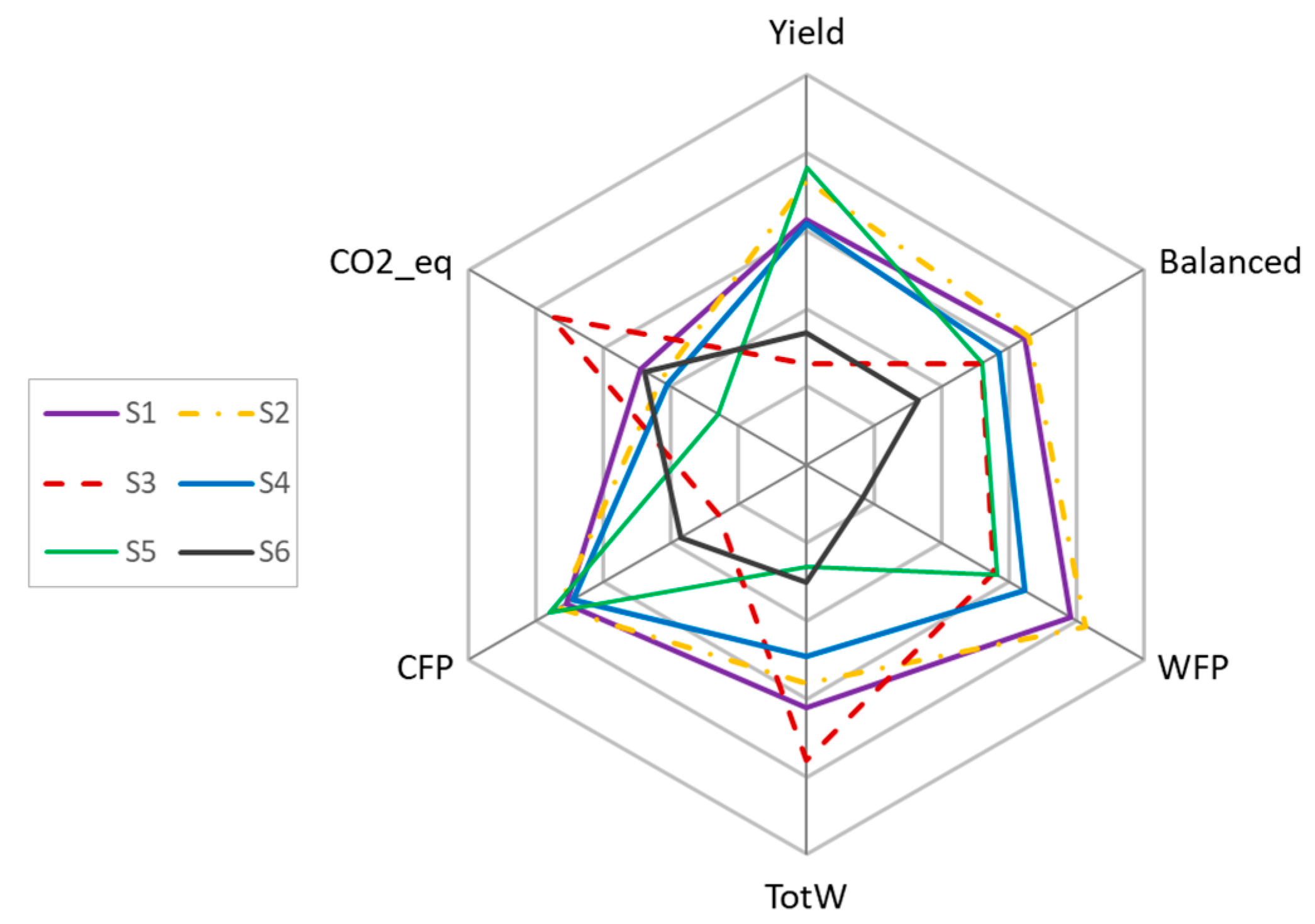
Figure 2 provides a synthetic visual representation of these results: each axis of the radar diagram corresponds to one decision profile, and the radial distance of each scenario from the centre reflects its composite AHP score under that profile. The radar makes the across-profile behaviour of each scenario immediately legible. S2 (01 Nov–Rainfed) and S5 (01 Nov–Irrigated) emerge as the two most convex polygons under ratio-metric and yield-oriented profiles, respectively, while S3 (15 Nov–Rainfed) bulges only along the CO₂_eq and TotW axes—the two absolute-metric profiles—and contracts sharply under all others. S6 (15 Nov–Irrigated) shows the smallest and most concave polygon overall, consistent with its Sensitive classification.

3.4. Switching Point Analysis and Ranking Stability

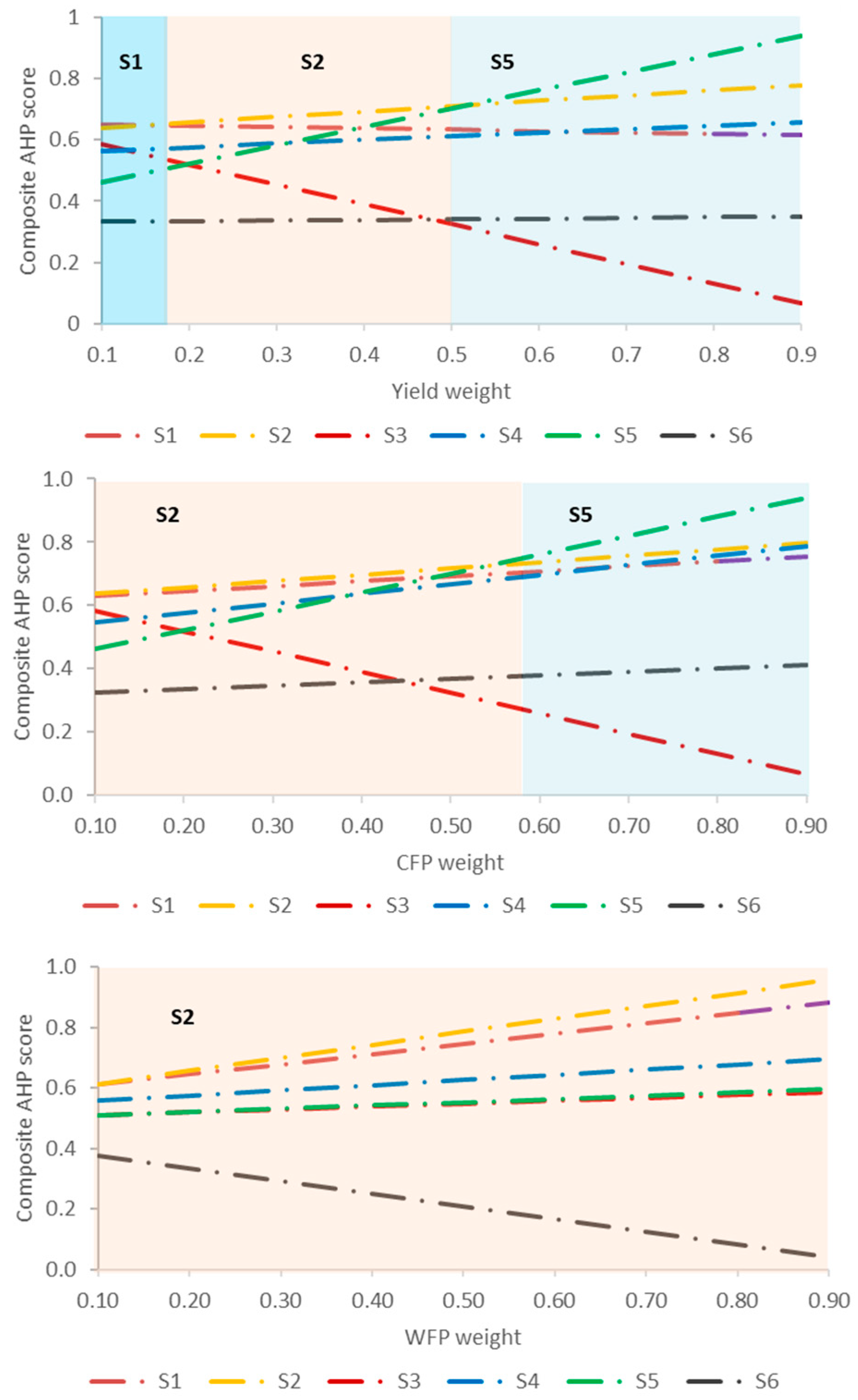
Switching point analyses (Equation (11)) quantify the robustness of the leading scenario as the dominant weight w_dom is varied from 0.10 to 0.90 in steps of 0.10 for three criteria: Yield (w₁), CFP (w₃), and WFP (w₅). Figure 3 reports the composite AHP score trajectories for all six scenarios as a function of each dominant weight. Along the Yield axis, two switching points are observed: S1 (15 Oct–Rainfed) leads at w₁ = 0.10 and is overtaken by S2 (01 Nov–Rainfed) at w1 = 0.20 (the discretisation in steps of 0.10 implies that the exact transition lies in the interval 0.10 < w₁ ≤ 0.20); S2 retains leadership up to w₁ = 0.50 and is overtaken by S5 (01 Nov–Irrigated) at w₁ = 0.60. Along the CFP axis, a single switching point is observed from S2 to S5 at w₃ = 0.60. Along the WFP axis, no switching point is observed within the investigated weight range: rainfed early-November sowing (S2) retains leadership throughout w₅ = 0.10 to 0.90, indicating exceptional robustness of this scenario under any priority given to water footprint efficiency. The numerical coincidence between the switching point on the Yield and CFP axes (w₁ = 0.60; w₃ = 0.60) and the dominant weight value used in the single-criterion profiles (w = 0.60) is incidental rather than designed: the switching point analysis sweeps the dominant weight independently across the full range [0.10, 0.90], and the location of the transition is determined entirely by the underlying indicator values; the proximity of these transitions to the profile-defining weight nevertheless usefully situates the symmetric weight scheme close to where rankings change.

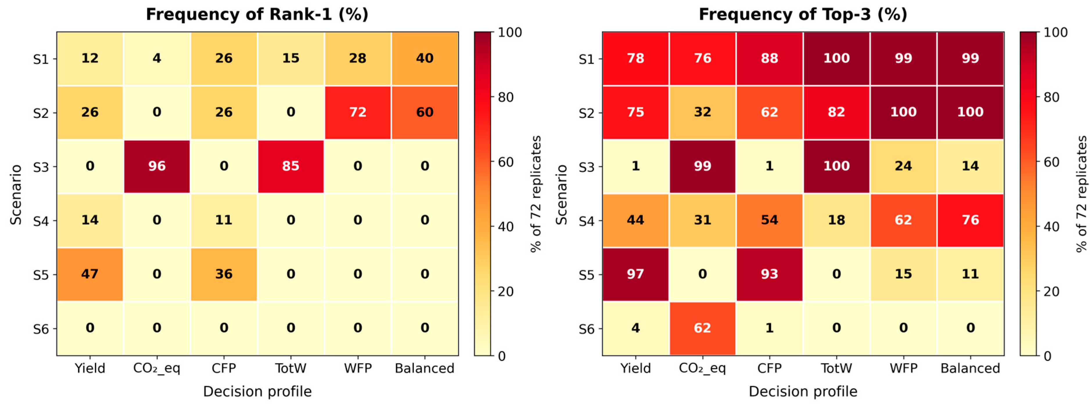
Figure 4 reports the empirical rank distributions obtained by repeating the full AHP procedure on each of the 72 simulation replicates underlying the mean values in Table 2. Three patterns emerge from the replicate analysis and qualify the mean-based rankings reported in Table 6.

First, the absolute–ratio indicator paradox is not an artefact of the average values: S3 (15 Nov–Rainfed) ranks first under the CO₂_eq-dominant profile in 96% of the replicates and under the TotW-dominant profile in 85% of them, while it never ranks first under any of the remaining four profiles. This bimodal behaviour—systematic leadership under absolute-metric profiles and systematic exclusion from the podium under yield- and ratio-metric profiles—persists across the full pedo-climatic variability of the dataset and is therefore a structural property of the indicator choice rather than a sensitivity of the mean.

Second, leadership under ratio-metric and balanced profiles is more distributed than the mean values alone would suggest. S2 (01 Nov–Rainfed) is the most frequent leader under the WFP-dominant profile at 72% of replicates and under the balanced profile at 60%, with S1 (15 Oct–Rainfed) taking the remainder in both cases (28% and 40%, respectively). Under the CFP-dominant profile, three scenarios alternate leadership across replicates (S5 at 36%, S1 and S2 at 26% each, and S4 at 11%), indicating that the mean-based first place of S5 reflects a narrow margin that is frequently reversed under specific pedo-climatic conditions. Under the Yield-dominant profile, S5 is the most frequent leader at 47%, but S2 wins in 26% of replicates and S4 in 14%.

Third, the top-three analysis reveals a different, more forgiving measure of robustness. S1 reaches the top three in 75% to 100% of the replicates under every single profile—a level of cross-profile consistency that no other scenario achieves. S2 is in the top three in at least 75% of the replicates under four of the six profiles (Yield-, TotW-, WFP-dominant, and balanced), drops to 62% under the CFP-dominant profile, and falls to 32% only under the CO₂_eq-dominant profile. Conversely, S6 (15 Nov–Irrigated) never reaches rank 1 and is in the top three in less than 5% of the replicates under five of the six profiles, confirming its classification as Sensitive across the full simulation dataset. S5 is in the top three in 93–97% of the replicates under the Yield- and CFP-dominant profiles but nearly absent from the top three under profiles driven by absolute environmental indicators, confirming its specialisation as a productivity-oriented option.

3.5. Indicator Dependence and Normalisation Sensitivity

The Pearson correlation matrix among the five performance indicators, computed on the pooled dataset of 432 observations (six scenarios × 72 replicates), is reported in

Table 8. Pearson correlation matrix among the five performance indicators, computed on the pooled dataset of 432 observations (6 scenarios × 72 replicates). Values are absolute correlation coefficients |r|; entries close to 1.00 indicate strong linear intercorrelation. The three absolute indicators (Yield, CO₂_eq, and TotW) show |r| ≥ 0.91 with each other; the two ratio indicators (CFP and WFP) show |r| from 0.31 to 0.67 with the absolute set, indicating that absolute and ratio quantities capture statistically distinguishable rather than redundant dimensions of sustainability.

Indicator	Yield	CO2_eq	CFP	TotW	WFP
Yield	1.00	0.99	−0.47	0.91	−0.66
CO2_eq	0.99	1.00	−0.50	0.91	−0.67
CFP	−0.47	−0.50	1.00	−0.42	0.35
TotW	0.91	0.91	−0.42	1.00	−0.31
WFP	−0.66	−0.67	0.35	−0.31	1.00

. The three absolute indicators (Yield, CO₂_eq, and TotW) are highly intercorrelated (|r| ≥ 0.91), reflecting the close coupling between productivity and absolute resource consumption in cereal systems with largely fixed management inputs. The two ratio indicators (CFP and WFP), by contrast, show |r| values from 0.31 to 0.67 with the absolute indicators, indicating that absolute and ratio quantities capture statistically distinguishable rather than redundant dimensions of sustainability. The dependence of CFP and WFP on Yield through their construction is the precise mathematical mechanism that produces the absolute–ratio inversion under opposite dominant profiles. The normalisation sensitivity test confirmed that the rank-1 leader is identical under min–max, vector, and AHP-eigenvector normalisation for five of the six decision profiles (Yield-, CFP-, TotW-, WFP-dominant, and balanced); the only profile sensitive to normalisation choice is the CO₂_eq-dominant profile, where the lowest-yielding scenario (15 November rainfed) leads under min–max but is overtaken by early-November rainfed under vector and eigenvector normalisations. The complete sensitivity outcome, including the composite score of the rank-1 leader and the relative gap (in %) between the rank-1 and rank-2 scenarios under each normalisation, is reported in

Table 9. Sensitivity of the rank-1 leader to the choice of normalisation. For each of the six decision profiles, the rank-1 leader scenario is reported under min–max normalisation (Equations (1) and (2)), vector normalisation (Equation (12)) and AHP-eigenvector normalisation (Equation (13)), together with the composite score of the leader and the relative gap (in %) between the rank-1 and rank-2 scenarios.

Decision Profile	Min–Max (Equations (1) and (2))	Vector (Equation (12))	AHP-Eigenvector (Equation (13))
Yield	S5 (0.761, +4.4%)	S5 (0.424, +1.2%)	S5 (0.173, +1.2%)
CO2_eq	S3 (0.759, +35.4%)	S2 (0.411, +0.1%)	S2 (0.168, +0.1%)
CFP	S5 (0.761, +3.6%)	S5 (0.432, +2.8%)	S5 (0.177, +2.8%)
TotW	S3 (0.759, +17.7%)	S3 (0.418, +0.7%)	S3 (0.171, +0.7%)
WFP	S2 (0.828, +5.4%)	S2 (0.419, +0.6%)	S2 (0.171, +0.6%)
Balanced	S2 (0.657, +1.4%)	S2 (0.416, +0.2%)	S2 (0.170, +0.2%)

. The gap analysis reveals a relevant pattern: under min–max normalization, the rank-1/rank-2 score gaps range from 1.4% (balanced) to 35.4% (CO₂_eq-dominant), whereas under vector and AHP-eigenvector normalisations, the same gaps are compressed to 0.1–2.8%. This indicates that the underlying dataset contains intrinsic near-ties between scenarios that min–max normalisation amplifies into more pronounced rank-1/rank-2 separations, while vector and proportional normalisation schemes preserve the near-tie structure. The single profile in which min–max and vector/eigenvector disagree on the rank-1 leader (CO₂_eq-dominant) is, accordingly, the profile for which the vector and eigenvector rank-1/rank-2 gap is the smallest (0.1%), meaning that the change of leader from 15 November to 1 November rainfed under those normalisations is itself marginal.

4. Discussion

4.1. The Absolute–Ratio Indicator Paradox

The systematic inversion between rankings under absolute and ratio indicators is the most substantive methodological result of the analysis. It is not an artefact of the weighting scheme or of specific weight values; it arises from the mathematical structure of the indicators themselves and operates through two parallel channels in the CWFP framework. For emissions, CO₂_eq is a per-hectare metric: in a system dominated by fixed management inputs (tillage, fertiliser manufacture and application, and seed), absolute emissions vary within a narrow band, and the lowest-yielding scenario is also the one with marginally lower absolute emissions because reduced biomass production slightly reduces N₂O emissions from residue. In contrast, CFP expresses emissions per unit of product, so it is most favourable in scenarios that achieve the highest yield for broadly comparable emission profiles.

The policy implication is direct. Rewarding low absolute per-hectare consumption, without reference to productivity, incentivises systems that consume fewer inputs per hectare mechanically, irrespective of whether this reflects genuine efficiency or merely reduced production. Under the CAP 2023–2027 eco-scheme framework [9], where reward mechanisms increasingly include climate- and GHG-related per-hectare reduction targets, this distinction has immediate operational consequences: an incentive based on absolute per-hectare GHG emissions would, in Capitanata, preferentially reward the least productive scenario, without improving either environmental performance per unit of product or total sectoral emissions once demand-driven cultivation of the displaced production is accounted for. The present analysis makes this choice operationally explicit and directly quantifies its ranking consequences across six theoretical decision profiles.

A parallel mechanism operates for water. TotW integrates green water (precipitation transpired by the crop) and blue water (direct irrigation plus indirect water embedded in input chains) within the cradle-to-gate boundary. Green water, which accounts for the dominant share of TotW in rainfed Mediterranean wheat, scales with the productive water use of the crop and is therefore lower in scenarios that fail to fully develop canopy and root system. Blue water varies less across scenarios and responds primarily to the supplemental irrigation applied (0, ≤60 mm). The lowest-yielding scenario (S3) thus attains the lowest TotW (5556 m³ ha⁻¹, Table 2) not because it achieves a better water footprint—in fact, its WFP (1.119 m³ kg⁻¹) is higher than that of the more productive S2 (1.078 m³ kg⁻¹)—but because it transpires less water cumulatively over a less developed growing season. WFP, by expressing water consumption per kilogram of grain, correctly rewards productive water use and penalises this outcome.

The present analysis operationalises a concern raised but not quantified in the LCA literature regarding the functional unit in agricultural systems [7,8], extending the discussion from LCA methodology into decision analysis. It establishes that the distinction between absolute and ratio indicators is not a technical detail but a first-order determinant of ranking outcomes, with measurable consequences for policy-relevant decisions. These findings should not be read as a general claim that ratio indicators are universally superior to absolute ones: the two indicator families answer different sustainability questions, and the choice between them depends on the policy objective. In contexts where stakeholders explicitly prioritise absolute caps on per-hectare consumption—for example, water abstraction limits in overexploited basins—absolute indicators must be used, and the analysis identifies S3 as the scenario that minimises those burdens. In contexts where the policy concern is environmental efficiency per unit of output, ratio indicators provide the more appropriate evaluation lens. More operationally, the choice between the two indicator families can be guided by the level at which the sustainability target is defined: area-based instruments (territorial GHG emission ceilings, basin-scale water withdrawal limits, and eco-scheme payments tied to per-hectare reductions) call for absolute indicators, whereas product-level instruments (carbon labelling, environmental product declarations, and supply-chain LCA benchmarks) call for ratio indicators. Where both policy levels are relevant, the two indicator families should be reported jointly rather than collapsed into a single composite score, since the present analysis shows that doing so masks a structural ranking divergence between the two.

4.2. Management Implications and Scenario-Specific Recommendations

The emergence of early-November sowing (S2 and S5) as the most consistently high-performing strategy across ratio-metric and balanced profiles confirms and quantifies the agronomic advantage of this sowing window in Capitanata, previously identified on an indicator-by-indicator basis [5,6]. The systematic analysis across six profiles shows that this advantage is not confined to single-criterion assessments but persists under most plausible weight combinations. Mid-November sowing (S3 and S6) is penalised by late-phenology exposure to heat and water stress during grain filling and scores first only under absolute-indicator profiles, where low productivity is rewarded. This dual behaviour of S3—first under the CO₂_eq- and TotW-dominant profiles, last under the Yield- and CFP-dominant profiles—is the most striking manifestation of the absolute–ratio paradox in the dataset.

The replicate analysis (Figure 4) refines this recommendation by distinguishing between leadership and consistency. S2 emerges as the most frequent leader under the WFP-dominant and balanced profiles that correspond to the stakeholder configurations most relevant for Mediterranean agronomic planning. S1 (15 Oct–Rainfed), while rarely the outright leader, is remarkably consistent: it appears in the top three under every profile in at least three quarters of the replicates and thus functions as a broadly acceptable fallback when stakeholder priorities are uncertain or likely to shift. S5 behaves as a productivity specialist—nearly always in the top three under yield- and CFP-oriented profiles and nearly always outside it under the others—and should therefore be recommended only when those priorities are clearly dominant.

The switching-point analysis adds operational value to the management recommendation. The transition from rainfed to irrigated early-November sowing (S2 to S5) along the Yield and CFP axes occurs at relatively high weight thresholds (w₁ = 0.60; w₃ = 0.60), indicating that supplemental irrigation becomes the preferred choice only under strongly productivity-oriented or carbon-efficiency-oriented priorities [24,25]. Conversely, along the WFP axis, no switching point is observed: rainfed early-November sowing (S2) retains the top-ranked position throughout the investigated range of w₅, from 0.10 to 0.90. This is a particularly robust finding, as it establishes that under any priority structure that emphasises water-footprint performance of durum wheat production, including balanced configurations, the same agronomic recommendation holds. For water-scarce Mediterranean agricultural systems, where water-footprint-oriented decision-making is increasingly common in both policy and farm-level practice, this robustness is a substantively meaningful result. The recommendations summarised above are environmental in scope only: irrigation decisions, in particular, have financial ramifications (irrigation infrastructure cost, water charges, and machinery utilisation) that are outside the present analysis but are central to actual farm-level decisions, as explicitly discussed in Section 4.3 and Section 5 the Conclusions.

4.3. Methodological Considerations and Limitations

The mean-based AHP rankings reported in Table 6 are one of two complementary views of the same dataset: the scenario-by-scenario summary of central tendencies, best suited to long-term management recommendations, and the replicate-based empirical rank distributions of Figure 4, best suited to understanding how those recommendations depend on the full pedo-climatic variability of the territory. The replicate analysis shows that the absolute–ratio indicator inversion operates at frequencies exceeding 85% across the 72 replicates—a pattern that characterises the joint structure of the indicators rather than any specific averaging operation—while also revealing that leadership margins are narrow under certain profiles (notably the CFP-dominant profile), where three scenarios alternate in the top position across different replicates. A natural further development would apply the same procedure to percentile-specific aggregates of the dataset—for example, to the 10th, 50th, and 90th percentiles of each indicator—enabling an explicit treatment of risk-aversion profiles.

A natural question raised by the present analysis is whether the AHP framework adds value beyond what could be inferred from inspection of the underlying simulation means alone (Table 2). The contribution operates on four distinct levels. First, the framework makes the otherwise implicit weighting of trade-offs explicit and reproducible: a reader inspecting Table 2 can intuit that 1 November rainfed sowing offers a favourable balance between yield and water use, but cannot translate that intuition into a quantitative ranking without committing to a specific weighting scheme—which AHP makes auditable through the pairwise matrices and the priority vectors. Second, the switching point analysis converts qualitative trade-offs into quantitative weight thresholds: it identifies the dominant-criterion weight at which leadership transitions from one scenario to another, information that is structurally absent from any tabular display of indicator means. Third, the replicate-based analysis shows that scenario means in Table 2 conceal substantial pedo-climatic variability: rank-1 leadership frequencies in Figure 4 reveal that the leadership reported in Section 3.3 holds at frequencies of 47–100% across 72 pedo-climatic contexts, a property that cannot be inferred from the raw means. Fourth, the absolute–ratio inversion documented in Section 3.3 is itself a non-obvious outcome of the framework: although the underlying indicator construction (CFP = CO₂_eq/Yield; WFP = TotW/Yield) is straightforward, the systematic reversal of rank-1 leadership across absolute-indicator and ratio-indicator profiles emerges only when the indicators are jointly weighted within a transparent MCDA scoring.

A distinctive methodological strength of the present analysis lies in the deliberate restriction of the agronomic decision space to two levers: sowing date and supplemental irrigation timing. Although this may appear a limitation relative to broader multifactor studies, it is precisely this parsimony that confers immediate operational relevance. Both variables are available to any Capitanata farmer without capital investment, machinery replacement, or changes in input procurement; they can be decided on a seasonal basis in response to evolving weather conditions, and they require no agronomic knowledge beyond what is already embedded in local farming practice. The finding that such a minimal set of decisions generates structurally stable, differentiated AHP rankings across six theoretical decision profiles and 72 pedo-climatic replicates demonstrates that the multi-criteria framework can extract actionable guidance from a deliberately simple agronomic space—a property that is rare in broader MCDA applications where wide decision spaces often produce rankings that are too stakeholder-specific to provide common guidance.

The contribution of the paper can be summarised at three complementary levels. First, at the indicator level, the analysis provides an explicit quantification of the absolute–ratio paradox in a Mediterranean wheat system, showing that the paradox not only exists but dominates AHP rankings under four of the six decision profiles and persists at frequencies above 85% across the pedo-climatic variability of the dataset. While AHP has been applied extensively in agricultural MCDA, the systematic examination of how absolute versus ratio environmental indicators affect AHP outcomes in a process-based crop simulation context appears not to have been a standard focus of previous applications. Second, at the procedural level, the paper demonstrates that perfectly consistent AHP pairwise matrices (CI = 0, CR = 0) can be constructed analytically from ratio-normalised indicator values—bypassing the subjective expert elicitation that historically dominates AHP practice and that introduces inconsistency issues. In the closely related study by Chandran et al. [26], who coupled DSSAT simulation output with TOPSIS for ranking cropping sequences under projected climate, AHP was used only as an auxiliary step for deriving criterion weights from expert judgement, yielding a consistency ratio of 0.06—acceptable under the Saaty threshold but not analytically 0. By contrast, the present framework applies AHP to scenario ranking directly with ratio-constructed matrices whose consistency is exact by design, a methodological property that we believe represents a useful refinement for AHP applications to crop simulation output. Third, at the integration level, the combination of ratio-based matrix construction, continuous switching-point analysis across the full weight range [0.10, 0.90] and replicate-based empirical rank distributions across 72 pedo-climatic realisations constitutes a self-contained, reproducible protocol for transparent multi-criteria evaluation of agronomic scenarios derived from process-based crop simulation output. Compared with expert-elicitation AHP applications—which tie the evaluation to a specific stakeholder panel—or fixed-weight MCDA applications [26], this protocol is fully deterministic once the underlying simulation and life-cycle assessment data are available, making it directly reproducible from any published dataset comparable to the one used here.

The symmetric weight scheme (0.60/0.10) is analytically transparent and makes stakeholder priorities directly interpretable, but it is a deliberate simplification relative to the full range of weight combinations that an arbitrary stakeholder might express. The switching point analysis partially addresses this limitation by tracing composite scores over the full range of dominant weights; however, a full sensitivity analysis with simultaneous variation of two or more weights would provide a more complete picture.

The analysis as currently constructed does not incorporate economic indicators (gross margin, cost of supplemental irrigation, and price volatility of inputs and outputs), which are central to farmer-level decision-making. Integrating an economic dimension would require consistent valuation of the five environmental indicators (e.g., via shadow prices for CO₂_eq and blue water) and is not trivial methodologically, but would substantially enhance the operational value of the analysis for farm-level advisory services.

Finally, while the analysis is calibrated specifically on the pedo-climatic and management context of the Capitanata plain, the methodology itself is fully transferable to other Mediterranean wheat systems, to other crops, and to other indicator sets, provided that a suitable simulation and LCA dataset is available. Applying the analytical approach to simulation datasets generated for different agro-ecological zones would allow systematic comparison of the geographical generality of the conclusions drawn here.

4.4. Sensitivity to Normalisation Choice and Indicator Dependence

Two natural questions concerning the multi-criteria framework—the statistical dependence among the five performance indicators and the sensitivity of rankings to the normalisation choice—were addressed through the dedicated diagnostic analyses. The five indicators are not statistically independent, and indeed cannot be: by construction, CFP and WFP, so that Yield enters as one of the five criteria and also as the denominator of two of the remaining four. The Pearson correlation matrix in Table 8 shows that the absolute indicators (Yield, CO₂_eq, and TotW) are highly intercorrelated, while the two ratio indicators (CFP and WFP) carry statistically distinguishable information rather than redundant yield content. The correlation pattern is consistent with the substantive interpretation of the framework: the indicator inversion documented in Section 3.3 reflects genuinely distinct dimensions of sustainability—absolute pressure per unit of land vs. efficiency per unit of product—and the inclusion of all five indicators is justified by their non-redundant statistical structure. The dependence of CFP and WFP on Yield through their construction does not invalidate the joint analysis but is the precise mathematical mechanism that produces the ranking divergence under absolute vs. ratio-dominant profiles. A restricted analysis using only the three structurally distinct indicators (Yield, CO₂_eq, and TotW) was also performed and preserved the qualitative finding that the lowest-yielding scenario leads under absolute-metric dominance, confirming that the indicator inversion is not an artefact of including ratio quantities in the criterion set.

The normalisation sensitivity test indicates that the rank-1 leader is invariant across the three normalisation schemes (min–max, vector, and AHP-eigenvector) for five of the six decision profiles: Yield-, CFP-, TotW-, WFP-dominant, and balanced. The CO₂_eq-dominant profile is the only profile that is sensitive to normalisation choice. This sensitivity is informative and consistent with the well-known property of min–max normalisation, which can amplify narrow absolute ranges (CO₂_eq varies by approximately 24 kg ha⁻¹ across the six scenarios, around 2% of the mean) into full 0–1 contrasts. Importantly, the absolute–ratio indicator inversion is not eliminated by changing normalisation: the TotW-dominant profile (the second absolute-metric profile) continues to select the lowest-yielding scenario as rank-1 leader under all three schemes. This confirms that the inversion phenomenon is a structural feature of the indicator pair (absolute vs. ratio) rather than a numerical artefact of min–max normalisation, although the magnitude of the effect on individual profiles is sensitive to this choice. A comprehensive uncertainty quantification combining alternative normalisations, alternative weight schemes, and stochastic input perturbation is left for future work.

Taken together, the indicator-dependence and normalisation-sensitivity analyses reinforce the central finding of the paper while explicitly bounding its scope. The structural inversion between absolute and ratio environmental indicators emerges robustly in the dataset, both in mean-based rankings and in the empirical rank distributions across 72 pedo-climatic replicates, and is not eliminated by alternative normalisation schemes. The magnitude of the effect on rankings under specific profiles is, however, sensitive to normalisation choice and to the inclusion or exclusion of strongly yield-dependent ratio indicators. Readers and downstream users of the framework should therefore interpret the rankings as one transparent instantiation of a structured multi-criteria evaluation, rather than as a definitive recommendation independent of these methodological choices.

5. Conclusions

The analytic hierarchy process with a symmetric weight scheme was applied to six durum wheat production scenarios in the Capitanata plain, evaluating five performance indicators across six theoretical decision profiles. Building on the long-standing recognition in the LCA literature that the choice of functional unit (per-area vs. per-product) influences environmental comparisons, the present analysis shows that this distinction translates into a substantive methodological decision within multi-criteria evaluation, with directly opposed ranking implications under absolute and ratio-dominant profiles. Under profiles that prioritise absolute per-hectare metrics, the lowest-yielding scenario paradoxically achieves first place because reduced productivity mechanically lowers per-hectare resource consumption without improving production efficiency. The choice between absolute and ratio indicators reflects different sustainability objectives; the former is appropriate when the policy concern is total local pressure per unit of land (basin-scale water depletion and area-based emission targets), the latter when the concern is environmental efficiency per unit of product. Neither is universally superior; they answer different questions, and indicator selection should follow the policy objective rather than methodological convenience.

Within the analytical setting examined here, early-November sowing emerges consistently as the most coherent agronomic option when sustainability is evaluated through ratio indicators or under balanced priorities. Rainfed early-November sowing is the most frequent leader under balanced and WFP-oriented priorities, combining a favourable water footprint with above-average yield and competitive carbon performance. Rainfed mid-October sowing, while rarely the outright leader, is the most broadly consistent option across the six profiles and may function as an acceptable fallback option when priorities are uncertain. Supplemental irrigation at flowering is environmentally justified—within the indicator set considered here—only when productivity-related objectives collectively dominate the decision, and its added value reflects yield stabilisation in dry years rather than systematic intensification. Mid-November sowing emerges as first-ranked only under absolute-metric profiles, where the ranking is driven by reduced per-hectare resource consumption associated with reduced yield rather than by intrinsic environmental superiority. These observations describe the ranking structure of the simulated dataset and are not, in themselves, prescriptive farm-level recommendations: farmer-level decisions on sowing date and supplemental irrigation are also determined by economic considerations (gross margin, input and output price volatility, irrigation cost, machinery, and infrastructure constraints) that are explicitly outside the scope of the present environmental multi-criteria analysis. The findings are therefore most directly relevant to environmental decision support and to the design of policy instruments and would benefit from coupling with an economic analysis before being translated into operational guidance for farmers.

Application of the same AHP procedure to the 72 simulation replicates underlying the scenario means extended the analysis to the full pedo-climatic variability of the 2013–2023 dataset. The resulting empirical rank distributions traced, for each scenario and each decision profile, the frequency with which leadership was achieved across distinct combinations of soil and climatic context, showing that the absolute–ratio indicator inversion and the leadership of rainfed early-November sowing under balanced and water-footprint-oriented profiles emerge consistently across the full dataset. The symmetric weight design, the analytical construction of perfectly consistent pairwise comparison matrices, the switching point analyses, and the replicate-based rank distributions, taken together, outline an operational approach to transparent multi-criteria decision analysis of agronomic scenarios derived from process-based crop simulation output. The methodology is in principle transferable to other Mediterranean crop systems, regions, and indicator sets for which comparable simulation and life-cycle assessment datasets are available, subject to the methodological caveats discussed (normalisation choice, indicator dependence, and absence of economic indicators). The specific scenario recommendations that emerge from the Capitanata dataset—the leadership of rainfed early-November sowing under ratio and balanced profiles and the appearance of mid-November sowing as first-ranked only under absolute-metric profiles—are bounded to the pedo-climatic, agronomic, and decadal (2013–2023) context examined here and should not be extrapolated as general agronomic guidance to other Mediterranean wheat-growing regions or to longer climate-change time horizons without rerunning the framework on locally appropriate simulation and life-cycle assessment data.

References

1. Martínez-Moreno, F.; Solís, I.; Noguero, D.; Blanco, A.; Özberk, İ.; Nsarellah, N.; Elias, E.; Mylonas, I.; Soriano, J.M. Durum Wheat in the Mediterranean Rim: Historical Evolution and Genetic Resources. Genet. Resour. Crop Evol. 2020, 67, 1415–1436. [Google Scholar] [CrossRef]
2. ISTAT. Censimento Agricoltura 2020. Available online: https://www.istat.it/notizia/censimento-agricoltura-2020-online-i-principali-dati/ (accessed on 1 March 2026).
3. Mäkinen, H.; Kaseva, J.; Trnka, M.; Balek, J.; Kersebaum, K.C.; Nendel, C.; Gobin, A.; Olesen, J.E.; Bindi, M.; Ferrise, R.; et al. Sensitivity of European Wheat to Extreme Weather. Field Crops Res. 2018, 222, 209–217. [Google Scholar] [CrossRef]
4. Trnka, M.; Olesen, J.E.; Kersebaum, K.C.; Skjelvåg, A.O.; Eitzinger, J.; Seguin, B.; Peltonen-Sainio, P.; Rötter, R.; Iglesias, A.; Orlandini, S.; et al. Agroclimatic Conditions in Europe under Climate Change. Glob. Change Biol. 2011, 17, 2298–2318. [Google Scholar] [CrossRef]
5. Garofalo, P.; Cammerino, A.R.B. Modeling the Performance of a Continuous Durum Wheat Cropping System in a Mediterranean Environment: Carbon and Water Footprint at Different Sowing Dates, Under Rainfed and Irrigated Water Regimes. Agriculture 2025, 15, 259. [Google Scholar] [CrossRef]
6. Padovan, G.; Martre, P.; Semenov, M.A.; Masoni, A.; Bregaglio, S.; Ventrella, D.; Lorite, I.J.; Santos, C.; Bindi, M.; Ferrise, R.; et al. Understanding Effects of Genotype × Environment × Sowing Window Interactions for Durum Wheat in the Mediterranean Basin. Field Crops Res. 2020, 259, 107969. [Google Scholar] [CrossRef]
7. Gan, Y.; Liang, C.; Wang, X.; McConkey, B. Lowering Carbon Footprint of Durum Wheat by Diversifying Cropping Systems. Field Crops Res. 2011, 122, 199–206. [Google Scholar] [CrossRef]
8. Mekonnen, M.M.; Hoekstra, A.Y. The Green, Blue and Grey Water Footprint of Crops and Derived Crop Products. Hydrol. Earth Syst. Sci. 2011, 15, 1577–1600. [Google Scholar] [CrossRef]
9. De Castro, P.; Miglietta, P.P.; Vecchio, Y. The Common Agricultural Policy 2021–2027: A New History for European Agriculture. Ital. Rev. Agric. Econ. 2020, 75, 5–12. [Google Scholar] [CrossRef]
10. Saaty, T.L. The Analytic Hierarchy Process: Planning, Priority Setting, Resource Allocation; McGraw-Hill: New York, NY, USA, 1980. [Google Scholar]
11. Donati, I.I.M.; Martelli, A.; Dalla Marta, A.; Garofalo, P.; Petrillo, A.; Altobelli, F. Using the Analytic Hierarchy Process to Prioritise Criteria to Enhance AquaCrop from the User Perspective. Italy Rev. Agric. Econ. 2026. [Google Scholar]
12. Cay, T.; Uyan, M. Evaluation of Reallocation Criteria in Land Consolidation Studies Using the Analytic Hierarchy Process (AHP). Land Use Policy 2013, 30, 541–548. [Google Scholar] [CrossRef]
13. AbdelRahman, M.A.E.; Yossif, T.M.H.; Metwaly, M.M. Enhancing Land Suitability Assessment through Integration of AHP and GIS-Based for Efficient Agricultural Planning in Arid Regions. Sci. Rep. 2025, 15, 31370. [Google Scholar] [CrossRef] [PubMed]
14. Mendas, A.; Delali, A. Integration of Multi-Criteria Decision Analysis in GIS to Develop Land Suitability for Agriculture: Application to Durum Wheat Cultivation in the Area of Mleta in Algeria. Comput. Electron. Agric. 2012, 83, 117–126. [Google Scholar] [CrossRef]
15. Todorović, M.; Mehmeti, A.; Cantore, V. Impact of Different Water and Nitrogen Inputs on the Eco-Efficiency of Durum Wheat Cultivation in Mediterranean Environments. J. Clean. Prod. 2018, 183, 1276–1288. [Google Scholar] [CrossRef]
16. Steduto, P.; Hsiao, T.C.; Raes, D.; Fereres, E. AquaCrop—The FAO Crop Model to Simulate Yield Response to Water: I. Concepts and Underlying Principles. Agron. J. 2009, 101, 426–437. [Google Scholar] [CrossRef]
17. Raes, D.; Steduto, P.; Hsiao, T.C.; Fereres, E. AquaCrop—The FAO Crop Model to Simulate Yield Response to Water: II. Main Algorithms and Software Description. Agron. J. 2009, 101, 438–447. [Google Scholar] [CrossRef]
18. Garofalo, P.; Parlavecchia, M.; Giglio, I.; Campobasso, I.; Ventrella, D. Developing a Software for Measuring Carbon and Water Footprint of Organic Durum Wheat Cultivation Systems: The Smart Future Organic Farming (SFOF) Project. In Proceedings of the XXV Convegno Nazionale di Agrometeorologia, Matera, Italy, 14–16 June 2023; AMS Acta: Amsterdam, The Netherlands, 2023; pp. 100–103. Available online: https://sfof-85d3d.web.app/#/Home (accessed on 1 March 2026).
19. FAO; IIASA. Harmonized World Soil Database, Version 2.0; FAO: Rome, Italy; IIASA: Laxenburg, Austria, 2023; ISBN 978-92-5-137499-3. [Google Scholar]
20. Regione Puglia. Regional Land Use Cover. 2011. Available online: https://pugliacon.regione.puglia.it/web/sit-puglia-sit/uso-del-suolo (accessed on 10 July 2024).
21. Agri4Cast. Joint Research Centre Data Portal. Available online: https://agri4cast.jrc.ec.europa.eu/DataPortal/ (accessed on 1 May 2024).
22. Trombetta, A.; Iacobellis, V.; Tarantino, E.; Gentile, F. Calibration of the AquaCrop Model for Winter Wheat Using MODIS LAI Images. Agric. Water Manag. 2016, 164, 304–316. [Google Scholar] [CrossRef]
23. Hyde, K.M.; Maier, H.R.; Colby, C.B. A Distance-Based Uncertainty Analysis Approach to Multi-Criteria Decision Analysis for Water Resource Decision Making. J. Environ. Manag. 2005, 77, 278–290. [Google Scholar] [CrossRef] [PubMed]
24. Oweis, T.; Zhang, H.; Pala, M. Water Use Efficiency of Rainfed and Irrigated Bread Wheat in a Mediterranean Environment. Agron. J. 2000, 92, 231–238. [Google Scholar] [CrossRef]
25. Karam, F.; Kabalan, R.; Breidi, J.; Rouphael, Y.; Oweis, T. Yield and Water-Production Functions of Two Durum Wheat Cultivars Grown under Different Irrigation and Nitrogen Regimes. Agric. Water Manag. 2009, 96, 603–615. [Google Scholar] [CrossRef]
26. Chandran, M.A.S.; Banerjee, S.; Mukherjee, A.; Nanda, M.K.; Venugopalan, V.K.; Laing, A.M.; Siddiqui, M.H.; Hossain, A. Coupling Crop Simulation Modelling and Multi-Criteria Decision Aid for Ranking the Sustainability of Cropping Sequences. Front. Sustain. Food Syst. 2023, 7, 1208283. [Google Scholar] [CrossRef]
Figure 1. Study area: the Capitanata plain (Foggia province, Apulia, southern Italy). Yellow = arable land; red outline = Foggia province boundary. Coordinates approximately 41°27′ N, 15°33′ E; the area extends over approximately 7000 km2 of the Capitanata plain, the principal durum wheat production zone in Italy.
Agriculture 16 01162 g001
Figure 2. Radar diagram of composite AHP scores (Equation (8)) across the six decision profiles, identified on each axis by its dominant indicator (Yield, CO2_eq, CFP, TotW, and WFP) or by the balanced profile. Axes represent the AHP score of each scenario under the six profiles, with the radial distance from the centre proportional to the composite score (range 0–1). Each closed polygon represents one scenario; a larger area indicates higher composite scores across the six decision profiles, while sharp inward indentations along single axes indicate poor performance under that specific profile.
Agriculture 16 01162 g002
Figure 3. Switching point analysis (Equation (11)) for the three selected dominant criteria: (above) Yield weight w1; (middle) CFP weight w3; (bottom) WFP weight w5. Each line represents the composite AHP score of one scenario as the dominant weight varies from 0.10 to 0.90 in steps of 0.10. Residual weight (1 − wdom) is distributed equally among the remaining four criteria. Coloured bands identify the top-ranked scenario at each weight level. Markers indicate the discrete weight values evaluated (step 0.10); the rank-1 transitions visible as crossings between curves therefore lie in the interval between consecutive markers rather than at the marker itself.
Agriculture 16 01162 g003
Figure 4. Ranking stability across the 72 simulation replicates. (Left panel): Frequency of Rank-1—percentage of replicates in which each scenario ranks first under each decision profile, identified on the x-axis by its dominant indicator (Yield, CO2_eq, CFP, TotW, and WFP) or by the balanced profile (equal weights). (Right panel): Frequency of Top-3—percentage of replicates in which each scenario appears within the top three ranks under each profile. Percentages are computed across the 72 replicates; each replicate corresponds to one (soil × climatic cell) combination from the 2013–2023 AquaCrop-GIS simulation dataset (10-year mean per combination). Numbers in each cell indicate the corresponding percentage.
Agriculture 16 01162 g004