Calibration of Discrete Element Parameters for Cassava Seed Stems Using the Tavares Model and GA-BP-GA Method

Abstract

Accurate discrete element method (DEM) simulations are essential for elucidating the precision seeding mechanisms and collision damage characteristics of cassava seed stem (CSS); however, such simulations are often limited by a lack of precise contact parameters. In this study, “Guire No. 7” CSS was selected as the research object to calibrate discrete element (DE) parameters by integrating physical experiments with DEM simulations. A stem model was constructed in EDEM software (Altair EDEM 2022) using three-dimensional scanning technology combined with SolidWorks 2024 modeling functions to investigate the influence of the model’s mesh face count on simulation accuracy. Physical experiments measured the average repose angle (RA) of the stems (30.28° ± 1.09°), along with parameters including the restitution coefficient for stem-stem and stem-steel plate collisions, and the coefficient of static friction between the stem and steel plate. The Plackett-Burman Design experiment was employed to screen parameters affecting the RA, and the steepest ascent experiment was conducted to determine their optimal value ranges. Using the RA as the response value, a Central Composite Design experiment combined with machine learning regression models was applied to optimize the influencing parameters and compare model performance. The results indicated that the GA-BP algorithm exhibited superior predictive capability compared to Support Vector Regression (SVR) and the BP neural network. Through optimization using a genetic algorithm (GA), the calibrated parameters were obtained: a stem-steel plate static friction coefficient (SFC) of 0.488, a stem-stem SFC of 0.489, and a stem-stem rolling friction coefficient of 0.131. The resulting simulated RA was 30.73°, yielding a relative error of 1.49% compared to the physically measured value. The GA-BP-GA method demonstrated better optimization performance than the central composite design experiment, thereby validating the accuracy of the calibrated contact parameters between stems. Furthermore, parameters for the Tavares model were calibrated through physical experiments on CSS, using collision damage force and collision damage energy (CDE) as validation indicators. The results showed that the relative errors for both collision damage force and CDE were less than 3%, which is within the acceptable error range, thereby confirming the validity of the calibrated DE parameters for the cassava seed stem.

1. Introduction

Cassava is a vital shrub-like crop characterized by woody stems typically reaching 2–5 m in height, with tuberous roots rich in starch and fiber [1,2]. The propagation of cassava is primarily achieved through stem cuttings, where in stems are cut into segments of 13–17 cm in length and planted in furrows either horizontally or vertically. Cassava cultivation offers several advantages, including low input costs and high yield potential. The tuberous roots, stems, and leaves are all utilizable. Beyond direct consumption, cassava can be processed into starch, bioethanol, and various organic chemicals, rendering it a versatile crop with extensive applications in the food and light industries [3,4]. In 2024, China’s cassava planting area exceeded 667,000 hectares, with an annual fresh tuber production surpassing 20 million tons. Through the promotion of improved varieties and the expansion of cultivated areas, the production potential of cassava continues to increase. However, the low level of mechanization in critical operations such as precision planting and efficient harvesting significantly constrains the further development of the industry. Currently, domestic production falls short of demand, making China a major importer [5]. Therefore, advancing cassava mechanization is crucial for safeguarding food security and alleviating pressure on energy supply chains. Precision planting is a critical step in cassava production. Traditional research methods encounter considerable difficulties in revealing the precision seeding mechanism of cassava and the collision damage mechanism of seed stems. Using numerical simulation technology to investigate these mechanisms at the microscopic level [6,7] can provide a theoretical basis for optimizing the key structures and operating parameters of cassava planters.

The discrete element method (DEM) is a computational simulation approach based on the assumption of discontinuity [8,9]. It is also an important tool for analyzing particle fracture phenomena, enabling the simulation of fracture processes of particles of different materials and scales within operating equipment, and has been widely applied in research on straw, fertilizer, and cottonseed [10,11,12]. For instance, Li et al. [10] simplified corn stalks into a breakable flexible fiber model composed of multi-segment sphere-cylinder units connected by nodal balls based on DEM, and calibrated parameters including the elastic ratio, plastic ratio, bending limit angle, and failure ratio using the steepest ascent experimental design. Du et al. [11] proposed a three-layer discrete element (DE) model based on the bonding enhancement method for tea stalks, and used the calibrated parameters to construct tensile and puncture models for corresponding simulation experiments. Despite the widespread application of the discrete element method (DEM) in the simulation of agricultural materials, existing calibration methods still exhibit deficiencies when applied to stem-like materials such as cassava seed stems (CSS). Hu et al. [13] pointed out that most DEM parameter calibration studies focus on spherical or near-spherical particles, whereas the non-spherical geometry of stem-like materials cannot be accurately characterized by agglomerates of spherical particles. Wang et al. [14] noted that existing alfalfa stem models simplify the stem as a rigid rod or basic flexible body, failing to simulate the plastic deformation, bending, and fracture of hollow stems, and lacking systematic calibration of contact parameters with key components such as flattening rolls. Xu et al. [15] observed that current studies ignore the differences in physical properties among different components of the whole rice plant and do not account for flexible characteristics. Furthermore, unique structures such as stem nodes or buds are often neglected in contact parameter calibration. Han et al. [16] further emphasized that simplification of stem surface morphology leads to systematic errors between simulated and measured repose angles, with relative errors reaching as high as 5%. Analysis shows that contact parameters vary significantly among different materials, and there are still few reports on the collision damage mechanism of cassava seed stem (CSS) based on DEM. Furthermore, existing research on the fracture of agricultural materials predominantly relies on bonding models, where sub-particles are typically spherical aggregates that differ considerably from actual morphologies [17]. In contrast, the Tavares model, as a particle replacement model, is widely used in the field of particle collision damage [18,19,20]. When simulating particle collision damage, this model uses polyhedral sub-particles, enabling a more accurate representation of particle damage behavior, and has been widely applied to study the motion mechanisms of multi-scale cohesive particle models. Chiaravalle et al. [21] pointed out in their comparison that the bonded particle model (BPM) suffers from high computational cost and complex parameter calibration. In contrast, the Tavares model, as a particle replacement model (PRM), not only enables efficient simulation of the breakage process for a large number of particles within a single time step but also more accurately represents the geometry of non-spherical materials through polyhedral particles, generating irregular fragments that are consistent with actual fracture morphology. More importantly, its inherent damage accumulation mechanism can track progressive damage under multiple subcritical impacts, providing support for simulating the repeated low-energy collisions experienced by cassava seed stems during precision seeding. Given the advantages of the Tavares model in characterizing the collision damage of non-spherical particles, it is also suitable for simulating the damage phenomena of non-spherical seed stems during operation, thus providing a more effective tool for analyzing the collision damage mechanism of agricultural materials.

To ensure the accuracy of DE parameter calibration, it is essential to establish a precise DE model of the material [22]. Current DE modeling of agricultural materials often simplifies real particles into simple geometric bodies. After obtaining the particle contour through three-dimensional scanning, the model is completed by filling it with particles. CSS are non-spherical and have a composite structure (composed of cortex, epidermis, xylem, and pith). In addition, the random distribution of buds and the complex shape make it difficult to simplify them into simple geometric bodies. Using a particle-filling method to construct the model would lead to excessively long simulation times. Considering the shape of the seed stem, representing it as a model with protruding buds is necessary to more accurately characterize its morphology [23,24,25]. Since non-spherical particle models differ significantly from traditional particle aggregate models in geometry, it is necessary to recalibrate the inter-stem contact parameters in DEM simulations. In the calibration of DE parameters for materials such as straw and fertilizer, response surface methodology (RSM) is commonly used to optimize significant parameters [26,27]. Furthermore, machine learning (ML), as an emerging nonlinear regression modeling method [28], has shown excellent predictive performance in data prediction and optimization. Tang et al. [29] pointed out that the traditional response surface methodology (RSM), based on low-order polynomial assumptions, struggles to accurately describe the strongly nonlinear relationship between the geometric parameters of a cyclone separator and its separation efficiency. In contrast, the GA-BP neural network, which globally optimizes the initial weights and thresholds using a genetic algorithm without requiring a pre-set model structure, reduces the average absolute deviation of predictions from 2.78% (RSM) to 1.96%, thereby improving prediction accuracy and robustness. Ma et al. [30] found that in the calibration of discrete element parameters for red clover seeds, RSM has limited capability in fitting complex interactions among parameters and is easily affected by the sample size of the experimental design. By contrast, the GA-BP model, leveraging its nonlinear mapping ability, increased the coefficient of determination R² from 0.9544 (RSM) to 0.9605, while significantly reducing both mean squared error and mean absolute error, overcoming the shortcomings of RSM in nonlinear modeling. Li et al. [31] demonstrated in the calibration of discrete element parameters for silage that the relative error after RSM optimization was 3.6%, whereas that after GA-BP-GA optimization was only 1.3%. The GA-BP method, which optimizes the neural network weights and topology via a genetic algorithm, exhibits stronger global search capability and higher parameter optimization efficiency than RSM. Diao et al. [32] compared BP, GA-BP, PSO-BP, and RSM models for the calibration of discrete element parameters of yam beans. The results showed that GA-BP outperformed RSM (R² = 0.9518) in terms of R² (0.9611), MSE (0.2112), and MAE (0.2809). The GA-BP effectively avoids the local optimum trap that RSM is prone to, while maintaining high fitting accuracy and stability under small sample data conditions. Therefore, the BP neural network optimized by a genetic algorithm (GA-BP) can avoid the drawback of RSM easily falling into local optima, and is more conducive to achieving a globally optimal parameter combination and higher fitting accuracy [33,34]. However, the application of this method in the calibration of DE simulation parameters for CSS has not been reported in the literature.

Therefore, this study focuses on the “Guire No. 7” CSS as the research object. The DE parameters were calibrated by combining physical experiments with DEM simulations. The plackett burman design and the steepest ascent experiment were employed to screen parameters affecting the RA and to determine their optimal value ranges. Using the RA as the response value, central composite design experiments and machine learning regression models (Support Vector Regression [SVR], BP neural network, and GA-BP algorithm) were applied to optimize the significant parameters, yielding the optimal combination. Based on this optimal parameter combination, physical validation experiments were conducted on the seed stems. The experimental and simulated values of the collision damage force and collision damage energy (CDE) were compared to verify the accuracy of the calibrated parameters.

2. Materials and Methods

2.1. Experimental Materials and Intrinsic Parameter Measurement

The experimental material was the “Guire No. 7” cassava seed stem, collected in early June 2025 from the planting base of the Agricultural Science Research Center of Guilin City in Ziyuan County, Guangxi, China. After harvest, the seed stems were cleaned of soil and debris. Seed stems free from pests and diseases, straight without curvature, and without damage were selected and cut into segments of 150 mm in length (each containing buds). All seed stem segments were stored in sealed boxes in a dark, well-ventilated room at 15–20 °C and 70–80% relative humidity to maintain freshness and moisture content.

The density of the seed stems was measured using the water displacement method [10,11,12]. A seed stem of mass $M_{\mathrm{ms}}$ was placed into a 250 mL graduated cylinder. To prevent the seed stem from floating after water addition, a 150 g calibration weight was fixed to the seed stem. Subsequently, 125 mL of water was added to the cylinder, and the total volume was recorded as $V_{\mathrm{zd}}$. The volume of the calibration weight alone $V_{\mathrm{fm}}$ was measured using the same method. The density of the seed stem was calculated using the following formula:

$${\rho }_{\mathrm{ms}}={\displaystyle \frac{M_{\mathrm{ms}}}{V_{\mathrm{zd}}-V_{\mathrm{fm}}-125}}$$

(1)

Based on 10 repeated measurements, the density of the seed stems was found to range from 693 to 747 kg/m³.

Compression tests were conducted using an ENS-DVU multifunctional texture analyzer to determine the Poisson’s ratio $\mu$ and shear modulus $K$ of the seed stems [10,11,12]. Poisson’s ratio was calculated as follows:

$$\mu ={\displaystyle \frac{\left|{\epsilon }_1\right|}{\left|{\epsilon }_2\right|}}={\displaystyle \frac{L_1-L_2}{H_1-H_2}}$$

(2)

where ${\epsilon }_1$ is the strain perpendicular to the loading direction; ${\epsilon }_2$ is the strain parallel to the loading direction; $L_1$ is the transverse dimension before compression, m; $L_2$ is the transverse dimension after compression, m; $H_1$ is the axial dimension before compression, m; and $H_2$ is the axial dimension after compression, m.

After obtaining Poisson’s ratio, the shear modulus $K$ was calculated:

$$K={\displaystyle \frac{F\cdot L}{2\left(1+\mu \right)\cdot S\cdot \Delta L}}$$

(3)

where $F$ is the maximum force sustained by the specimen during the elastic deformation stage, N; $L$ the initial length of the specimen, m; $S$ is the cross-sectional area of the specimen, m²; and $\Delta L$ is the difference in specimen length before and after compression, m.

Based on 10 repeated measurements, the Poisson’s ratio of the CSS was determined to range from 0.37 to 0.45, and the shear modulus ranged from 16.40 to 17.60 MPa.

2.2. Physical Experiment Methods

2.2.1. Measurement of the Angle Repose for CSS

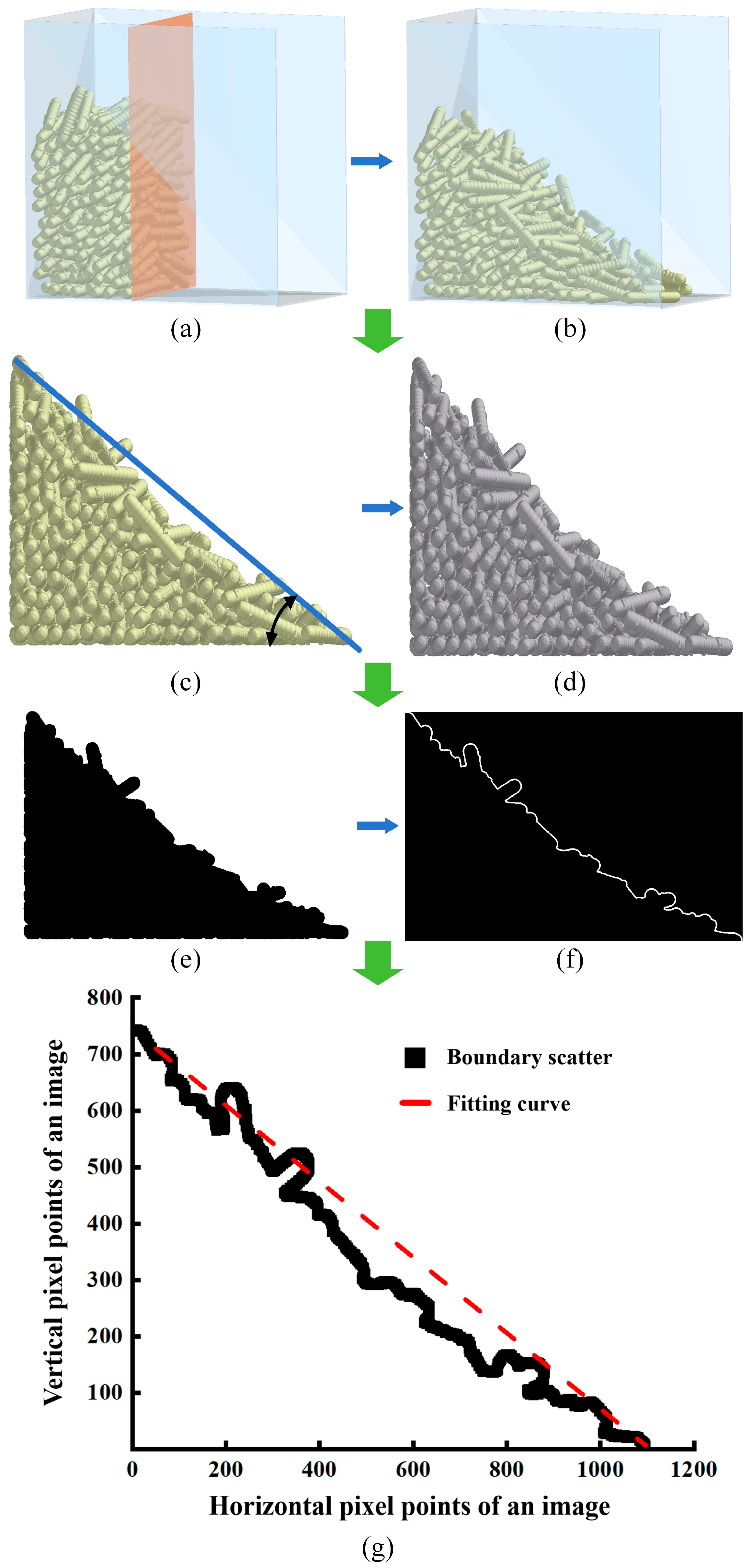
The side-wall collapse method was used to measure the repose angle (RA) of the seed stems. The side-wall and the middle baffle of the device were made of steel plates, and the baffle could move freely in the vertical direction under external force. A total of 250 seed stems were placed into the space between the side wall and the baffle. After the seed stems came to rest, the baffle was withdrawn upward, allowing the seed stems to flow toward the unobstructed side. Once the flow stopped, the angle of the slope formed by the seed stem pile was measured. Using a protractor to measure the RA introduced large errors; therefore, an image processing method was adopted [35]. The experiment was repeated ten times, and the average RA was 30.28° with a coefficient of variation of 3.61%. The measurement of the RA in the simulation followed the same method as in the physical experiment.

2.2.2. Static Friction Coefficient of CSS

The static friction coefficient (SFC) is defined as the ratio of the maximum static friction force to the normal pressure at the contact surface [36,37]. The SFC for seed stem-seed stem and seed stem-steel plate were measured using an inclined plane apparatus. To measure the seed stem-steel plate SFC, the steel plate was fixed to the measuring plane of the inclined plane apparatus with nuts. A seed stem was placed axially along the length direction of the measuring plane on the steel plate. The measuring plane was slowly rotated clockwise, and the rotation was stopped when the seed stem just began to slide on the steel plate. The inclination angle of the measuring plane at this moment was measured with a protractor. The SFC between the seed stem and the steel plate was then calculated using Equation (4). For the measurement of the seed stem-seed stem SFC, the steel plate was replaced with a uniformly arranged layer of seed stems.

$$f_s=\tan \alpha$$

(4)

where $f_s$ is the SFC; and $\alpha$ is the critical angle at which sliding commences, (°).

The SFC experiment was repeated ten times. The measured SFC between the seed stem and the steel plate ranged from 0.39 to 0.63. Similarly, the measured SFC between seed stems ranged from 0.42 to 0.66.

2.2.3. Rolling Friction Coefficient of CSS

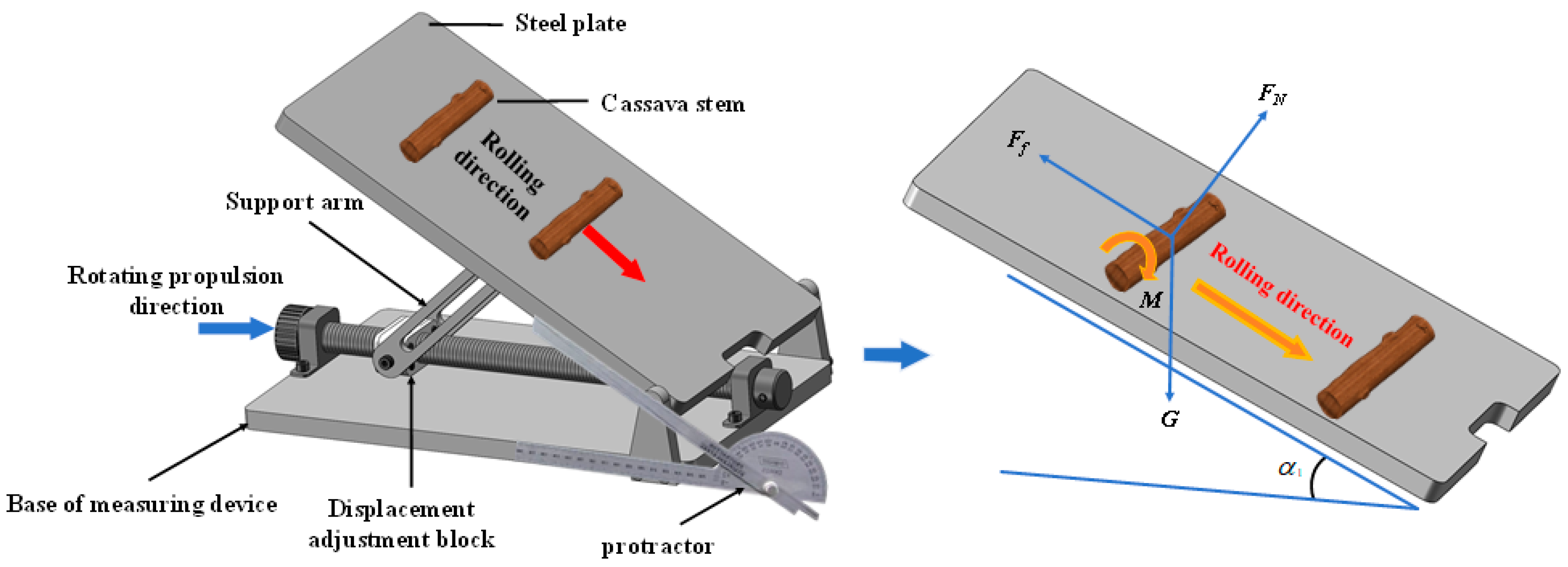
The rolling friction coefficient (RFC) refers to the resistance caused by the deformation at the contact surface when an object rolls without slipping or tends to roll on the surface of another object [36,37]. A seed stem was placed radially on the steel plate along the length direction of the measuring plane. The measuring plane was slowly rotated clockwise, and the rotation was stopped when the seed stem just began to roll purely on the steel plate. The inclination angle of the measuring plane at this moment was measured with a protractor. The forces acting on the seed stem in the measuring device are shown in Figure 1. During rolling, the rolling friction moment on the inclined plane is proportional to the normal support force from the inclined plane. When the inclined plane reaches a certain angle, the seed stem tends to roll.

$$M=f\cdot F_N$$

(5)

$$F_N-G\cos {\alpha }_1=0$$

(6)

$$Gr\sin {\alpha }_1-M=0$$

(7)

$$f={\displaystyle \frac{M}{F_N}}=r\tan {\alpha }_1$$

(8)

where $M$ is the rolling friction couple moment, N·m; f is the RFC; $F_N$ is the normal support force exerted by the inclined plane on the seed stem, N; $G$ is the gravitational force acting on the seed stem, N; ${\alpha }_1$ is the critical angle for rolling friction of the seed stem, (°); and $r$ is the radius of the seed stem, m.

The RFC experiment was repeated ten times. The measured RFC between the seed stem and the steel plate ranged from 0.13 to 0.25. Similarly, the measured RFC between seed stems ranged from 0.09 to 0.17.

2.2.4. Restitution Coefficient

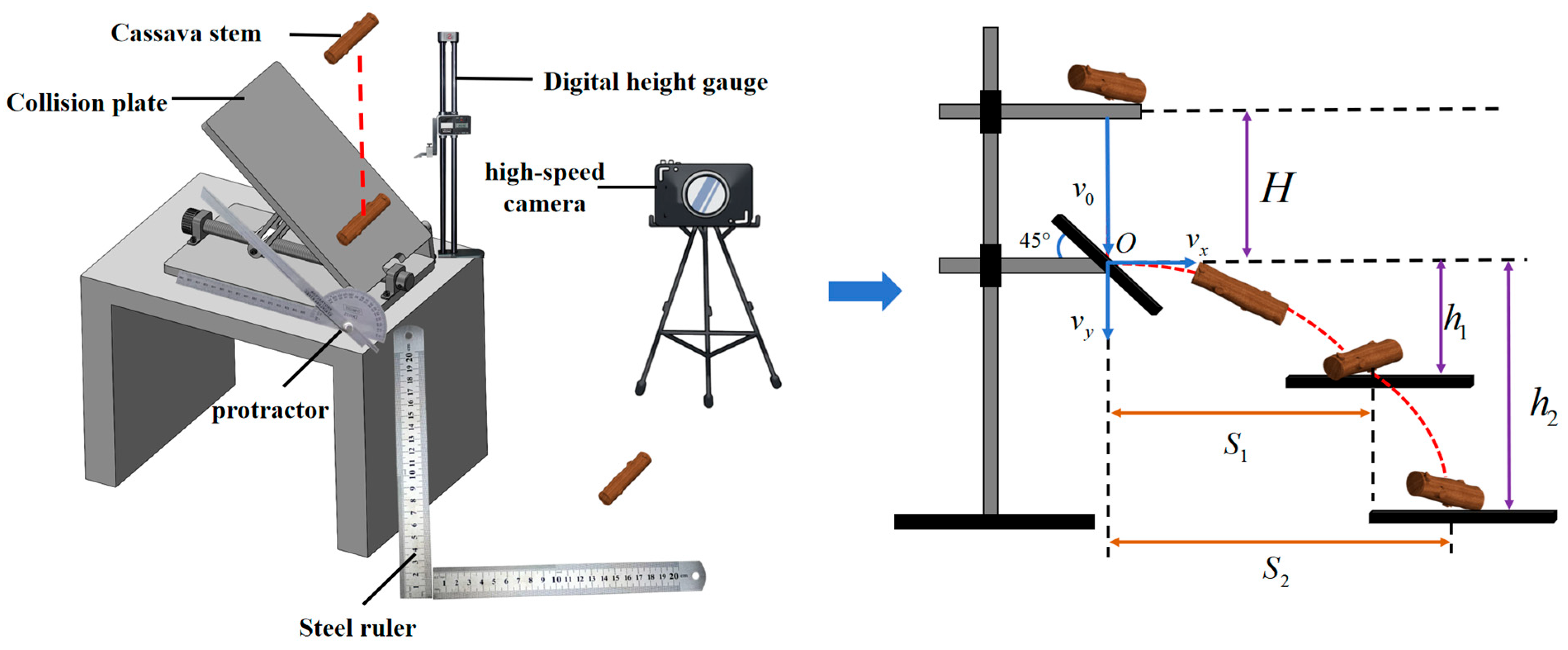
The Restitution Coefficient (RC) [36,37] is a parameter that quantifies the ability of an object to recover its original shape after deformation. It is defined as the ratio of the instantaneous normal separation velocity at the contact point at the end of collision to the normal approach velocity before collision. The measurement principle is illustrated in Figure 2. During the experiment, a seed stem was released from a discharge port positioned at a height H above the impact plate, undergoing free-fall motion before colliding with the impact plate below. The inclination angle of the impact plate was adjustable. Neglecting air resistance, the seed stem was subjected only to gravity during this process. Based on kinematic principles, the instantaneous velocity of the seed stem immediately prior to contact with the impact plate was determined.

$$\mathrm{a}\left\{\begin{array}{l}{v}_0=gt\\ H={\displaystyle \frac{1}{2}}g{t}^2\end{array}\right.$$

(9)

where $v_0$ is the velocity of seed stem immediately prior to collision, m/s; and $t$ is the free-fall time of seed stem, s.

According to Equation (9), the instantaneous velocity $v_0$ of the seed stem immediately prior to collision at point O on the impact plate is:

$$v_0=\sqrt{2gH}$$

(10)

Assuming that the trajectory of the seed stem after collision with the impact plate follows a projectile motion, i.e., a uniform linear motion in the horizontal direction with a velocity component of $v_x$ and a uniformly accelerated linear motion in the vertical direction with a velocity component of $v_y$, the post-collision trajectory of the seed stem forms a parabolic path. According to the principles of projectile motion, the following can be derived:

$$\left\{\begin{array}{l}s=v_x{t}_1\\ h=v_{y}t+{\displaystyle \frac{1}{2}}g{t}_1^2\end{array}\right.$$

(11)

where $t_1$ is the flight time of the seed stem after collision, s; $s$ is the horizontal displacement of the seed stem, m; and $h$ is the free-fall height of the seed stem after collision, m.

Since the time from the free fall of the seed stem from the discharge port to its collision with the impact plate is difficult to measure accurately, determining the horizontal velocity component $v_x$ and vertical velocity component $v_y$ after rebound becomes challenging. To overcome this difficulty, two experiments were conducted by adjusting the height of the collecting tray. A high-speed camera was used to capture the rebound trajectories of the CSS under two different collecting tray heights. The horizontal displacements $s_1$, $s_2$ and vertical displacements $h_1$, $h_2$ were measured respectively. The calculation formulas for the horizontal velocity component $v_x$ and vertical velocity component $V_y$ of the seed stem were derived as follows:

$$\left\{\begin{array}{l}{v}_x=\sqrt{{\displaystyle \frac{g{s}_1{s}_2(s_1-s_2)}{2(h_1{s}_2-h_2{s}_1)}}}\\ v_y={\displaystyle \frac{h_1{v}_x}{s_1}}-{\displaystyle \frac{g{s}_1}{2v_x}}\end{array}\right.$$

(12)

According to the definition of the RC, the following can be obtained:

$$e={\displaystyle \frac{v_n}{v_{0n}}}={\displaystyle \frac{\sqrt{v_x^2+v_y^2}\cos (\theta +\arctan \frac{v_y}{v_x})}{v_0\sin \theta }}$$

(13)

where $e$ is the RC; $v_n$ is the normal separation velocity after collision, m/s; $v_{0n}$ is the normal approach velocity before collision, m/s; and $\theta$ is the inclination angle of the impact plate, (°).

Based on ten repeated measurements, the RC for stem-stem collisions was determined to range from 0.3 to 0.5, while that for stem-steel plate collisions ranged from 0.3 to 0.6.

2.3. Establishment of the Discrete Element Model for CSS

2.3.1. Tavares Model Theory

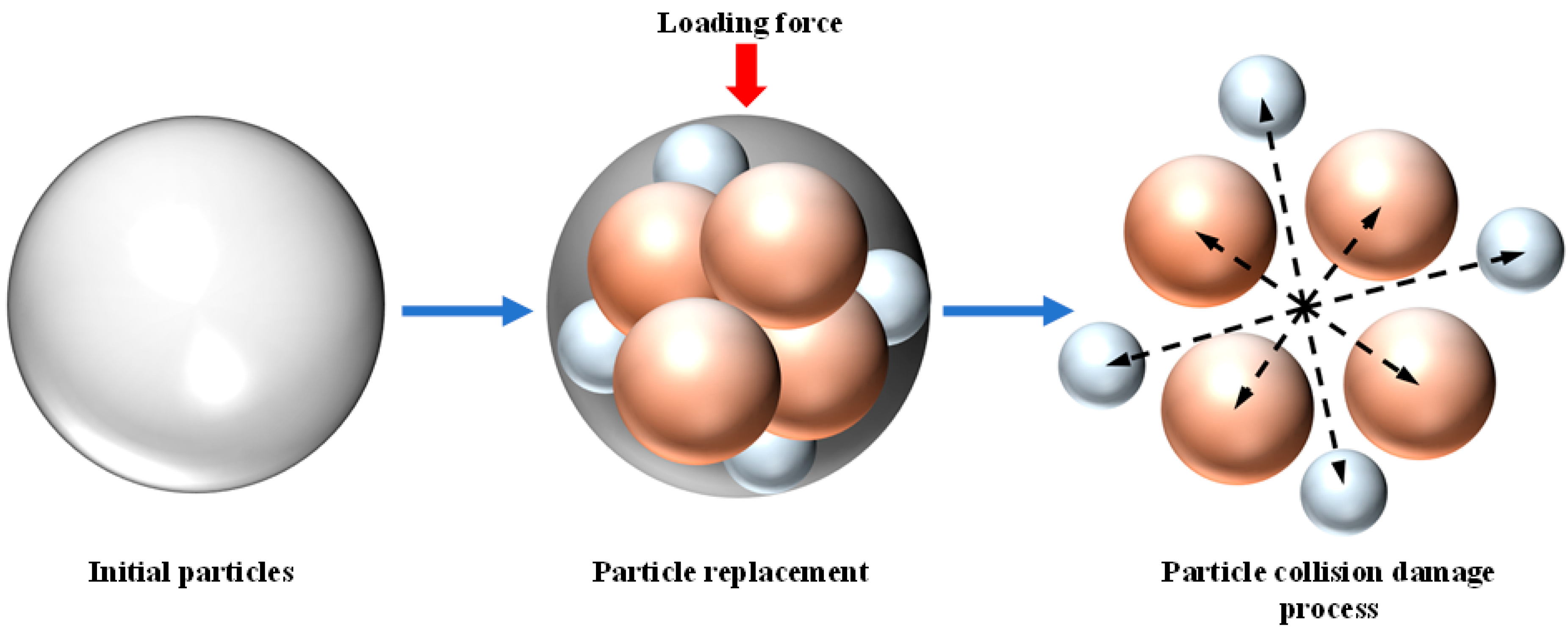
As shown in Figure 3, the Tavares model describes the principle of material damage through the particle collision process. The condition for particle collision damage depends on the intrinsic material properties as well as the forces exerted by the geometry and surrounding materials on the particle [18,19,20]. The relationship between the CDE energy and the normal and tangential energies is given by the following equations:

$$E_k=E_n+c_t{E}_t$$

(14)

where $E_n$ and $E_t$ are the normal energy and tangential energy, respectively, $\mathrm{J}$; $c_t$ is the tangential energy coefficient.

Furthermore, each particle possesses a specific CDE, which is calibrated based on the particle size. This energy, denoted as $P(E)$, is defined as:

$$P(E)={\displaystyle \frac{1}{2}}[1+\mathrm{erf}({\displaystyle \frac{\ln E^{*}-\ln E_{50}}{\sqrt{2}\sigma }})]$$

(15)

$$E^{*}={\displaystyle \frac{E_{\max }E}{E_{\max }-E}}$$

(16)

where $\mathrm{erf}$ is the error function; $E_{50}$ is the median CDE, $\mathrm{J}$; $\sigma$ is the standard deviation of the CDE; and $E_{\max }$ is the upper truncation value of the distribution, $\mathrm{J}$.

The median particle CDE $E_{50}$ is defined as follows:

$$E_{50}={\displaystyle \frac{E_{\infty }}{1+k_p/k_{st}}}[1+{({\displaystyle \frac{d_0}{d_p}})}^{\varphi }]$$

(17)

where $E_{\infty }$ is the minimum CDE at the maximum particle size, $\mathrm{J}$; $d_0$ is the median particle size, m; $\varphi$ is the fitting parameter for CDE; $d_p$ is the particle size, m; $k_p$ is the particle stiffness, GPa; and $k_{st}$ is the contact stiffness, GPa.

If a particle does not break under an impact, it will accumulate damage, which reduces its subsequent fracture energy. Once the impact energy exceeds the particle’s current fracture energy, the particle breaks and is replaced by a group of new sub-particles. Until the particle breaks, the particle’s damage fracture energy ${E’}_f$ and the previous fracture energy $E_f$ satisfy the following relationship:

$${E’}_f=E_f(1-D)$$

(18)

$$D={[{\displaystyle \frac{2r}{(2r-5D+5)}}\times {\displaystyle \frac{e{E}_k}{E_f}}]}^{{\displaystyle \frac{2\gamma }{5}}}$$

(19)

$$e={\displaystyle \frac{1}{1+k_p/k_s}}$$

(20)

where $D$ is the damage coefficient; $e{E}_k$ is the effective stress energy, $\mathrm{J}$; $\gamma$ is the damage coefficient; $e$ is the energy ratio; $k_p$ is the particle stiffness, GPa; $k_s$ is the particle contact stiffness, GPa.

The degree of breakage for small particles is expressed by $t_{10}$. This parameter represents the proportion of small particles that, after breakage, are smaller than one-tenth of the size of the material to be broken, as shown in the following equation:

$$t_{10}=A[1-\exp (-b{\displaystyle \frac{e{E}_k}{E_f}})]$$

(21)

where $A$ and $b$ are impact parameters fitted by experiments.

2.3.2. The Discrete Element Model for CSS

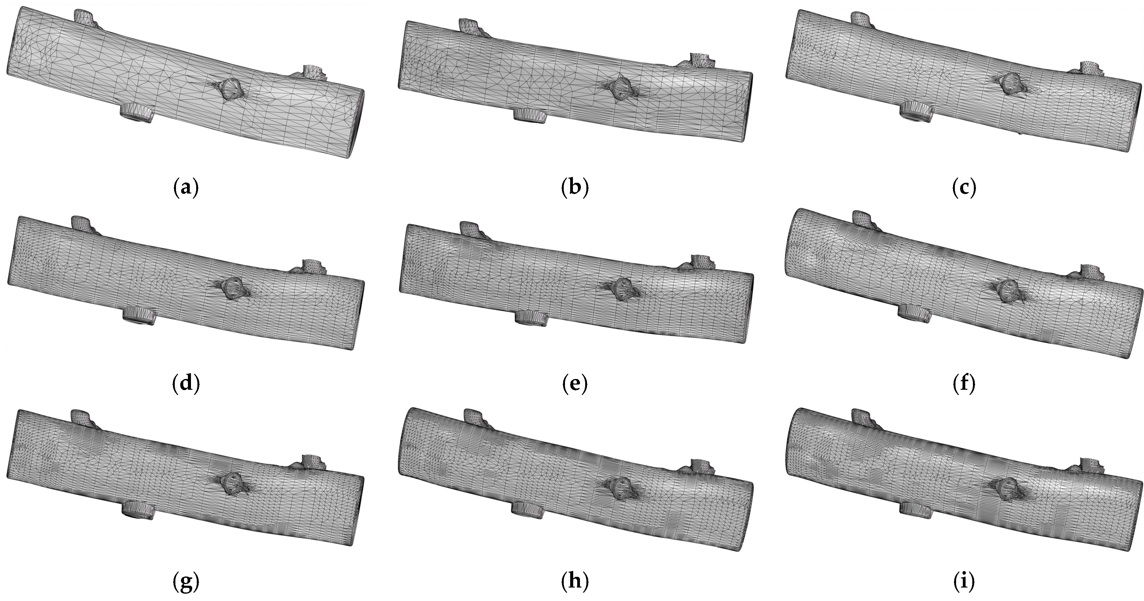
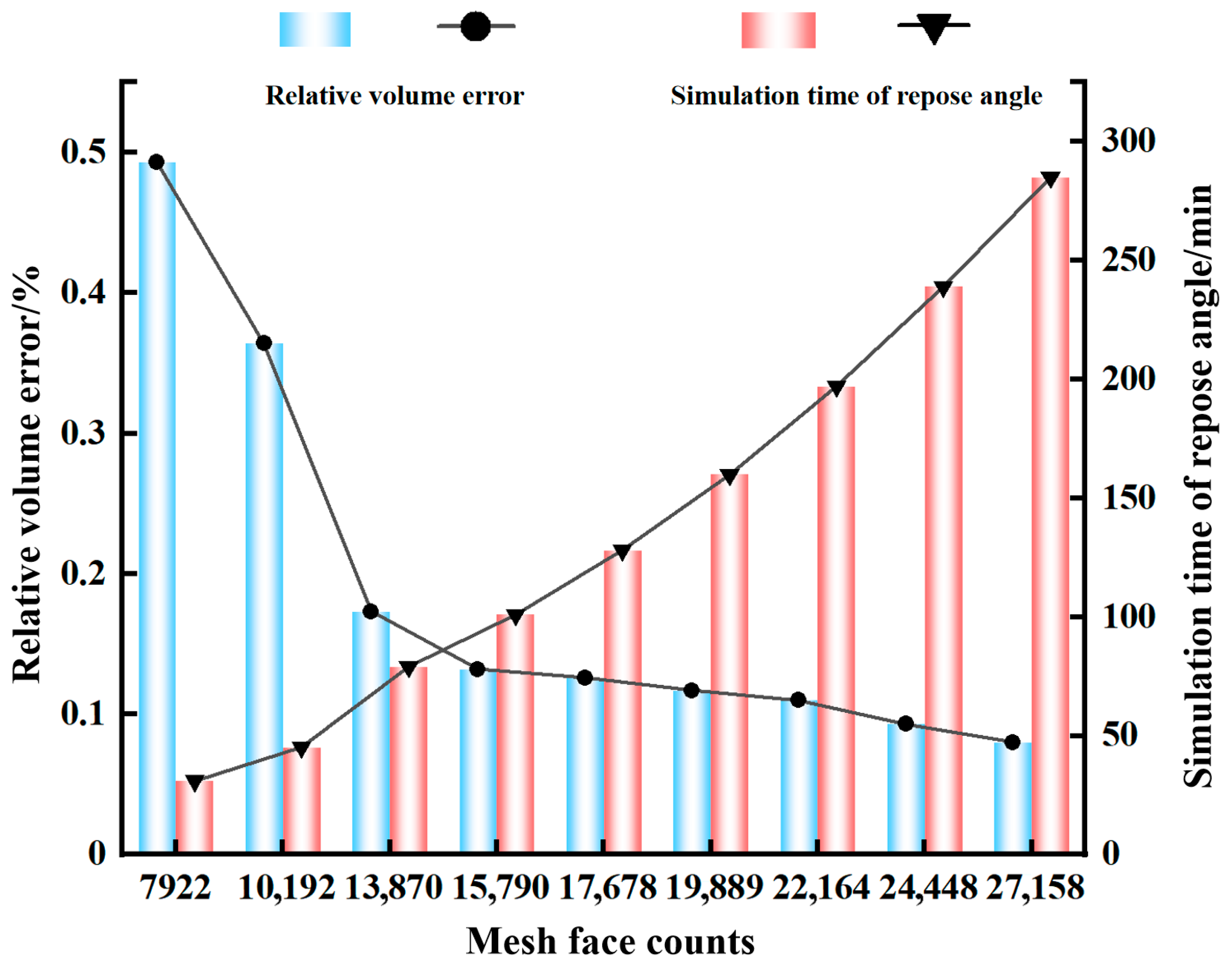
Considering that cassava seed stems exhibit an irregular cylindrical morphology with randomly distributed buds on the surface, traditional spherical particle agglomerate models cannot accurately characterize their true geometry and contact mechanical behavior. Therefore, simplifying the seed stem into a non-spherical polyhedral particle composed of multiple triangular planes can preserve the true contour and contact characteristics during motion and collision to the greatest extent, thereby improving the accuracy of discrete element simulations [23,24]. As shown in Figure 4, the contour model of the seed stem was obtained using three-dimensional scanning technology, and the number of mesh faces of the model was reduced using software to construct the DE model of the seed stem. The procedure was as follows: (1) A scanner was used to scan the contour of the seed stem to obtain point cloud data. (2) The point cloud data were processed to obtain a contour model of the seed stem. (3) The contour model was imported into SolidWorks 2024 software, where the meshing function was employed to reduce the mesh faces of the seed stem model, and the model was exported in STL format. The seed stem model was imported into EDEM, and the simulation time step was determined according to the Rayleigh time step criterion, taking 20% of the critical Rayleigh time step to ensure the stability of the discrete element simulation. Preliminary repose angle tests were conducted using parameters from the literature, and the results were imported into Origin software for plotting. As shown in Figure 5, the volume relative error of the model decreased continuously with the increasing number of mesh faces. After the mesh face count reached 15,790, the decreasing trend of the volume error slowed down significantly and gradually stabilized. The simulation time increased almost linearly with the number of mesh faces. When the mesh face count exceeded 15,790, the simulation became time-consuming, while the improvement in model accuracy was limited. Considering the variation pattern of volume error and simulation efficiency in Figure 5, a mesh face count of 15,790 represents the critical point achieving the optimal balance between simulation accuracy and computational efficiency. This choice ensures that the geometric accuracy of the model meets the simulation requirements while avoiding efficiency degradation caused by excessive mesh refinement. Therefore, the CSS model with a mesh face count of 15,790 was selected for subsequent discrete element simulations.

2.3.3. Establishment of the Simulation Model for the RA of CSS

Based on the CSS DE model, an RA measurement device with the same structure and dimensions as the experimental setup was established [10,11,12]. The device was saved as an STP file and imported into EDEM. A total of 250 CSS segments were statically generated. After the seed stem pile became stable, the baffle was moved to form the RA. The simulation device for the RA and the formed RA are shown in Figure 6.

2.4. Experimental Design and Methodology

2.4.1. RSM

(1) The Plackett–Burman design experiment was conducted using Design-Expert software (Design-Expert version 13) to screen the intrinsic parameters of the seed stems (Density X1, Poisson’s ratio X2, Shear modulus X3) and contact parameters (RC for seed stem-seed stem collisions X4, RC for seed stem-steel plate collisions X5, SFC for seed stem-steel plate X6, SFC for seed stem-seed stem X7, RFC for seed stem-steel plate X8, and RFC for seed stem-seed stem X9), with the goal of identifying the parameters that significantly affect the RA. Based on the experiments and relevant references [10,11,12,27], the values of the parameters to be calibrated were obtained, as shown in

Table 1. Coding of factors for Plackett–Burman design.

Number	Factor	Encoding
		−1	0	1
1	X1	693	720	747
2	X2	0.37	0.41	0.45
3	X3	16.42	17.14	17.86
4	X4	0.3	0.4	0.5
5	X5	0.3	0.45	0.6
6	X6	0.39	0.51	0.63
7	X7	0.42	0.54	0.66
8	X8	0.13	0.19	0.25
9	X9	0.09	0.13	0.17

.

(2) The steepest ascent experiment can quickly determine the optimal range of the factors. Using the significant factors identified by the Plackett–Burman design experiment (seed stem-steel plate SFC X6, seed stem-seed stem SFC X7, and seed stem-seed stem RFC X9), their corresponding level intervals were equally divided into 6 parts. The non-significant parameters were set at their middle levels, and the RA simulations were conducted. With the objective of minimizing the relative error, the upper and lower bounds of the central composite design response surface (RS) experiment were determined.

$$e={\displaystyle \frac{\left|y-z\right|}{y}}\times 100\%$$

(22)

where $e$ is the relative error, (%); $y$ is the experimentally measured RA of the seed stems, (°); and $z$ is the simulated RA of the seed stems, (°).

(3) Based on the results of the steepest ascent experiment, a central composite design (CCD) RS method was employed to conduct RS experiments and determine the optimal parameters. The value ranges obtained from the steepest ascent experiment were used as the upper and lower limits for the RS experiments. Non-significant parameters were set at their intermediate levels. The coding of the significant parameters and simulation factors is presented in

Table 2. Factors and coded levels for central composite design.

Encoding	Factor
	X6	X7	X9
−1.682	0.405274	0.435274	0.0950913
−1	0.438	0.468	0.106
0	0.486	0.516	0.122
1	0.534	0.564	0.138
1.682	0.566726	0.596726	0.148909

.

2.4.2. Machine Learning Regression Modeling

Using the same dataset employed in the RSM, regression modeling was performed in MATLAB 2025b using Support Vector Regression (SVR), BP neural network, and Genetic Algorithm-optimized Back Propagation (GA-BP) algorithms to identify the optimal regression fitting approach [28,29,30,31].

(1) Support Vector Regression (SVR): SVR identifies a regression hyperplane that minimizes the distance between all data points in a dataset and this hyperplane. Assuming the sample set is denoted as (x1, y1), (x2, y2), …, (xi, yi), where x ∈ Rn, y ∈ R, and R represents the set of real numbers. By replacing y with a function f(x) of x, the relationship between y and x in the sample set can be expressed by the following equation:

$$f(x)=\omega \cdot x+b$$

(23)

where $\omega$ and $b$ are the coefficients of the hyperplane.

If the original data exhibits a good fit with the Support Vector Regression model, then the following condition holds:

$$\begin{array}{c}\min \frac{1}{2}{‖\omega ‖}^2\\ \mathrm{s}\cdot \mathrm{t}.\left\{\begin{array}{c}\omega \cdot x_n+b-y_n\le \epsilon \\ y_n-\omega \cdot x_n-b\le \epsilon \end{array}\right.,n=1,2,\dots ,l\end{array}$$

(24)

where $\epsilon$ is an arbitrary positive number.

However, actual data often cannot fully satisfy the above strict constraints. To overcome this limitation, slack variables ${\xi }_n$ and ${\xi }_n^{*}$ are introduced. Meanwhile, a penalty parameter $C$ is introduced to balance model complexity and fitting error, resulting in the following optimization form:

$$\begin{array}{c}\min {\displaystyle \frac{1}{2}}{‖{\displaystyle \omega }‖}^2+C{\displaystyle \sum _n^l({\xi }_n+{\xi }_n^{*})}\\ \mathrm{s}\cdot \mathrm{t}.\left\{\begin{array}{l}\begin{array}{c}\omega \cdot x_n+b-y_n\le \epsilon +{\xi }_n\\ y_n-(\omega \cdot x_n+b)\le \epsilon +{\xi }_n^{*}\end{array}\\ {\xi }_n,{\xi }_n^{*}\ge 0\end{array}\right.,n=1,2,\dots ,l\end{array}$$

(25)

where $C$ is the penalty coefficient; and ${\xi }_n$, ${\xi }_n^{*}$ are the slack variables.

By introducing the Lagrange multiplier, Equation (21) can be transformed into:

$$f(x)=\omega \cdot x+b={\displaystyle \sum _{n=1}^l(an-a{n}^{\ast })(x_n,x)}+b$$

(26)

where $a_n$ and $a_n^{\ast }$ are the Lagrange multipliers corresponding to the samples, and most of them take the value of zero.

For nonlinear regression problems, the data can be mapped to a high-dimensional feature space using a kernel function $K(x_i,x)$. Therefore, Equation (22) can be transformed into:

$$f(x)={\displaystyle \sum _{n=1}^l(an-a{n}^{\ast })K(x_n,x)}+b$$

(27)

In summary, the SVR type was set to ε-SVR regression, with the loss function parameter set to 0.05 and the gamma function value set to 0.2.

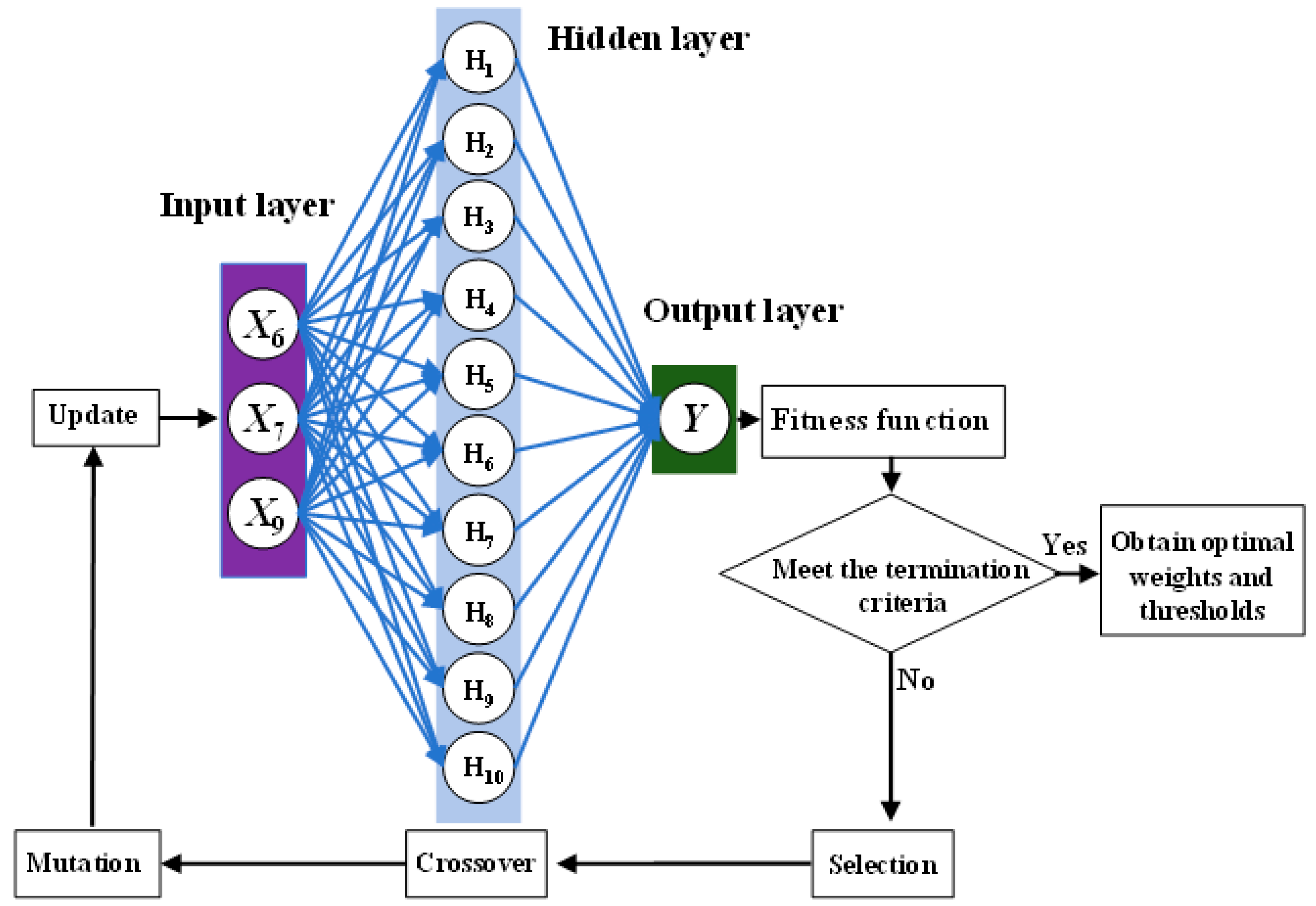
(2) BP Neural Network: For the BP neural network, an increasing number of layers enhances the function fitting capability; however, too many layers may lead to overfitting and make the model difficult to converge. Therefore, a three-layer BP neural network was constructed, comprising an input layer, a single hidden layer, and an output layer. The input layer was configured with three neurons, corresponding to the stem-steel plate SFC (X₆), the stem-stem SFC (X₇), and the stem-stem RFC (X₉), while the repose angle was set as the output layer. The transfer function of the hidden layer was the hyperbolic tangent sigmoid function (tansig), and the transfer function of the output layer was the linear function (purelin). The Levenberg–Marquardt (LM) algorithm was selected for model training, with a training target error of 0.0001, a learning rate of 0.005, and a maximum number of training steps of 100. The number of nodes in the hidden layer was determined using a trial-and-error method.

$$s_{11}={\sqrt{n_{11}+l}}_{11}+c_{11}$$

(28)

where $n_{11}$ and $l_{11}$ are the number of neurons in the input layer and output layer, respectively; $c_{11}$ is a constant ranging from 1 to 11; and $s_{11}$ ranges from 3 to 13.

(3) Genetic Algorithm-Back Propagation (GA-BP) Model: Given that the randomly initialized parameters of the BP network can lead to slow convergence and a tendency to fall into local minima, a genetic algorithm (GA) was employed to perform a global search before executing the BP neural network. The initial weights and thresholds of the hidden and output layers were optimized to provide a better evolutionary starting point for the BP network, thereby improving the fitting accuracy of the repose angle prediction model. The key parameters of the GA at this stage were set as follows: the number of evolution iterations was 200, and the population size was 150. The selection function was geometric ranking with a selection coefficient of 0.12, which enhances the selection pressure on high-fitness individuals while maintaining population diversity. The crossover rate was set to 0.9 to ensure sufficient global search, and the mutation rate was set to 0.1 to maintain a certain local perturbation capability and prevent premature convergence. Through selection, crossover, and mutation operations, the individual population was iteratively refined. The initial weights and thresholds obtained after GA optimization were then assigned to the BP neural network for updating until the termination criterion was met.

2.4.3. Genetic Algorithm Optimization

For an unknown nonlinear function, it is challenging to accurately determine the function extremum solely from input-output data. Leveraging the nonlinear optimization capability of genetic algorithms, the trained GA-BP prediction model was used as the fitness function [31], and the global search ability of GA was again employed to perform reverse optimization of the three significant contact parameters (the stem-steel plate SFC (X₆), the stem-stem SFC (X₇), and the stem-stem RFC (X₉)), with the target of the actual repose angle of the seed stems measured by physical experiments (30.28°). The GA parameters at this stage were set as follows: the number of evolution iterations was 150, and the population size was increased appropriately to 200 to enhance the coverage capability of the parameter space. The selection function was still geometric ranking, but the selection coefficient was adjusted to 0.08 to slightly reduce the selection pressure and avoid premature convergence to a local optimum. The crossover rate was maintained at 0.9, and the mutation rate at 0.1. Unlike the first-stage GA, the optimization objective at this stage was to make the simulated repose angle approach the measured target value, thereby directly obtaining the optimal combination of discrete element contact parameters, rather than optimizing the weights and thresholds of the neural network.

2.4.4. Data Analysis and Processing

Design-Expert software was employed for experimental design and data processing. The predictive performance of the RSM and machine learning models was evaluated using the coefficient of determination (R²), mean squared error (MSE), and average absolute deviation (AAD) [28,29,30,31].

3. Results and Analysis

3.1. PBD Test Results and Analysis

The Plackett-Burman Design (PBD) test scheme and results are presented in

Table 3. Experimental scheme and results of the Plackett–Burman design.

Number	Factor									Stacking Angle θ11 /(°)
	X1	X2	X3	X4	X5	X6	X7	X8	X9
1	747	0.45	16.40	0.5	0.6	0.63	0.42	0.13	0.09	29.14
2	693	0.45	17.60	0.3	0.6	0.63	0.66	0.13	0.09	38.33
3	747	0.37	17.60	0.5	0.3	0.63	0.66	0.25	0.09	45.06
4	693	0.45	16.40	0.5	0.6	0.39	0.66	0.25	0.17	33.42
5	693	0.37	17.60	0.3	0.6	0.63	0.42	0.25	0.17	34.57
6	693	0.37	16.40	0.5	0.3	0.63	0.66	0.13	0.17	47.43
7	747	0.37	16.40	0.3	0.6	0.39	0.66	0.25	0.09	25.73
8	747	0.45	16.40	0.3	0.3	0.63	0.42	0.25	0.17	39.22
9	747	0.45	17.60	0.3	0.3	0.39	0.66	0.13	0.17	40.25
10	693	0.45	17.60	0.5	0.3	0.39	0.42	0.25	0.09	21.27
11	747	0.37	17.60	0.5	0.6	0.39	0.42	0.13	0.17	30.86
12	693	0.37	16.40	0.3	0.3	0.39	0.42	0.13	0.09	20.16
13	720	0.41	17.00	0.4	0.45	0.51	0.54	0.19	0.13	31.8

, and the analysis of variance for the effects of parameters on the RA is provided in

Table 4. Analysis of variance for the Plackett–Burman design experimental results.

Source of Variance	Sum of Squares	Degree of Freedom	F	p	Contribution Rate/%	Significance Ranking
Models	837.08	9	29.74	0.0329 *	/	/
X1	18.95	1	6.06	0.1329	2.24	6
X2	0.3960	1	0.1266	0.7560	0.05	9
X3	19.35	1	6.19	0.1306	2.29	5
X4	6.63	1	2.12	0.2826	0.78	7
X5	37.95	1	12.14	0.0734	4.48	4
X6	320.95	1	102.63	0.0096 **	37.90	1
X7	252.08	1	80.61	0.0122 *	29.77	2
X8	3.97	1	1.27	0.3770	0.47	8
X9	176.79	1	56.53	0.0172 *	20.88	3
Residual	6.25	2
Sum	846.98	12

Note: * indicates significant impact (0.01 ≤ p ≤ 0.05), and ** indicates extremely significant impact (p < 0.01).

. The results indicated that the stem-steel plate SFC (X₆), the stem-stem SFC (X₇), and the stem-stem RFC (X₉) had significant effects on the RA, while the remaining parameters exhibited no significant influence. The PBD involved nine factors, with a basic experimental run count of 12 (excluding center points). The main-effect model consumed 9 degrees of freedom, leaving only 2 residual degrees of freedom. Low residual degrees of freedom elevate the critical F-value for significance tests, potentially leading to the omission of factors with minor effects. To improve statistical reliability, one center point was added to the 12 PBD runs, resulting in a total of 13 runs, and the residual degrees of freedom were calculated to be 3. The inclusion of the center point also provides an independent estimate of pure error, making the analysis of variance more reliable. Furthermore, the contribution rates of the three significant factors totalled 88.55% (Table 4), and their effect values were substantially larger than those of the non-significant factors. These three factors exhibited monotonic trends in the subsequent steepest ascent experiment and all showed extremely significant effects (p < 0.01) in the CCD response surface experiment, which is fully consistent with the screening conclusions from the PBD. Therefore, the overall results of parameter screening are reasonable and reliable.

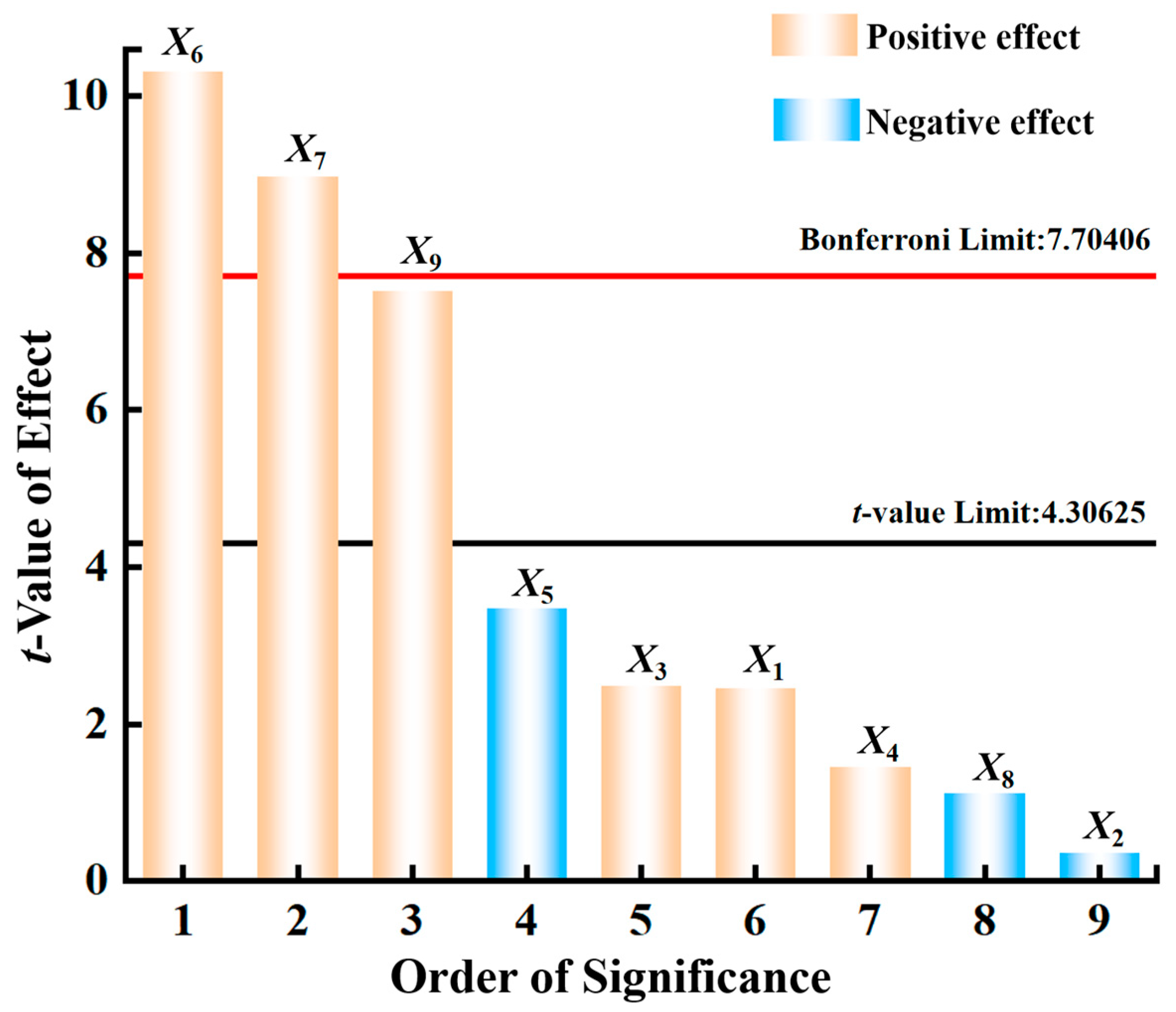
A t-test for the effects of each factor was conducted using Design-Expert software, as shown in Figure 7. Based on the confidence levels of the factors [10,11,12], the significant factors were selected for further investigation. The t-test results revealed that the order of significance of the factors on the RA was: stem-steel plate SFC (X₆) > stem-stem SFC (X₇) > stem-stem RFC (X₉). The p-values for the stem-stem SFC (X₇) and the stem-stem RFC (X₉) were less than 0.05, indicating that these factors had significant effects on the target. The p-value for the stem-steel plate SFC (X₆) was less than 0.01, indicating an extremely significant effect. This conclusion was further supported by the t-test values from the Pareto chart. Moreover, the effect values of X₆, X₇, and X₉ on the RA were positive. The first-order model fitted between the factors and the RA was expressed as follows:

$$\begin{array}{l}{\theta }_{11}=-84.74236+0.046543X_1-4.54167X_2+2.11667X_3+7.43333X_4-11.85556X_5\\ +57.46296X_6+57.29167X_7-9.58333X_8+95.95833X_9\end{array}$$

(29)

3.2. Steepest Ascent Test Results and Analysis

Based on the PBD test results, the non-significant parameters affecting the RA were set at their intermediate levels. The three significant parameters were subjected to a steepest ascent test using the factor levels derived from the PBD test. The relative error between the simulated and measured angles of repose was calculated, and the results are presented in

Table 5. Steepest climb test design and results.

Number	Factor			$\mathbf{Stacking} \mathbf{Angle} {\mathit{\theta }}_{11}$ /(°)	Relative Error e/%
	X6	X7	X9
1	0.390	0.420	0.090	20.63	31.87
2	0.438	0.468	0.106	25.79	14.83
3	0.486	0.516	0.122	31.42	3.77
4	0.534	0.564	0.138	36.79	21.50
5	0.582	0.612	0.154	41.35	36.56
6	0.630	0.660	0.170	44.26	46.17

. The results indicated that as the stem-steel plate SFC (X₆), the stem-stem SFC (X₇), and the stem-stem RFC (X₉) increased, the simulated RA increased continuously. The relative error of the RA initially decreased and then increased, with the smallest relative error observed in the third test group. Therefore, the levels near those selected in the third test group, specifically the levels used in the second, third, and fourth test groups, were chosen for subsequent RS analysis experiments, and an RS analysis regression model was established.

3.3. RS Analysis Test Results and Analysis

The central composite design (CCD) test scheme and results are presented in

Table 6. Experimental scheme and results of the central composite design.

Number	Factor			Stacking Angle /(°)
	X6	X7	X9
1	0.438	0.468	0.106	25.63
2	0.534	0.468	0.106	33.48
3	0.438	0.564	0.106	29.72
4	0.534	0.564	0.106	35.62
5	0.438	0.468	0.138	27.61
6	0.534	0.468	0.138	33.53
7	0.438	0.564	0.138	31.24
8	0.534	0.564	0.138	38.67
9	0.405274	0.516	0.122	26.17
10	0.566726	0.516	0.122	38.29
11	0.486	0.435274	0.122	27.25
12	0.486	0.596726	0.122	34.92
13	0.486	0.516	0.0950913	27.81
14	0.486	0.516	0.148909	33.28
15	0.486	0.516	0.122	32.12
16	0.486	0.516	0.122	29.65
17	0.486	0.516	0.122	30.73
18	0.486	0.516	0.122	29.85
19	0.486	0.516	0.122	31.12
20	0.486	0.516	0.122	29.36
21	0.486	0.516	0.122	29.92
22	0.486	0.516	0.122	31.43
23	0.486	0.516	0.122	30.19

. Design-Expert software was employed to analyze the results, and a quadratic regression model was established. After eliminating factors with insignificant effects on the quadratic regression model, the analysis of variance (ANOVA) for the optimized regression model is presented in

Table 7. Analysis of variance for the optimized regression model of the central composite design.

Source of Variance	Sum of Squares	Degree of Freedom	Mean Square	F	p
Models	249.03	4	62.26	73.42	<0.0001 **
X6	165.09	1	165.09	194.69	<0.0001 **
X7	57.00	1	57.00	67.21	<0.0001 **
X9	18.28	1	18.28	21.55	0.0002 **
X62	8.66	1	8.66	10.21	0.0050 **
Misfit	15.26	10	0.8462		0.5128
Residual	8.46	18	0.8480	0.9953
Error	6.80	8	0.8502
Sum	264.29	22

Note: ** indicates extremely significant impact (p < 0.01).

. The resulting regression equation is as follows:

$${\theta }_{12}=40.46441-239.04203X_6+42.56006X_7+72.30530X_9+320.44975X_6^2$$

(30)

3.4. Effects of Interaction Factors on the RA

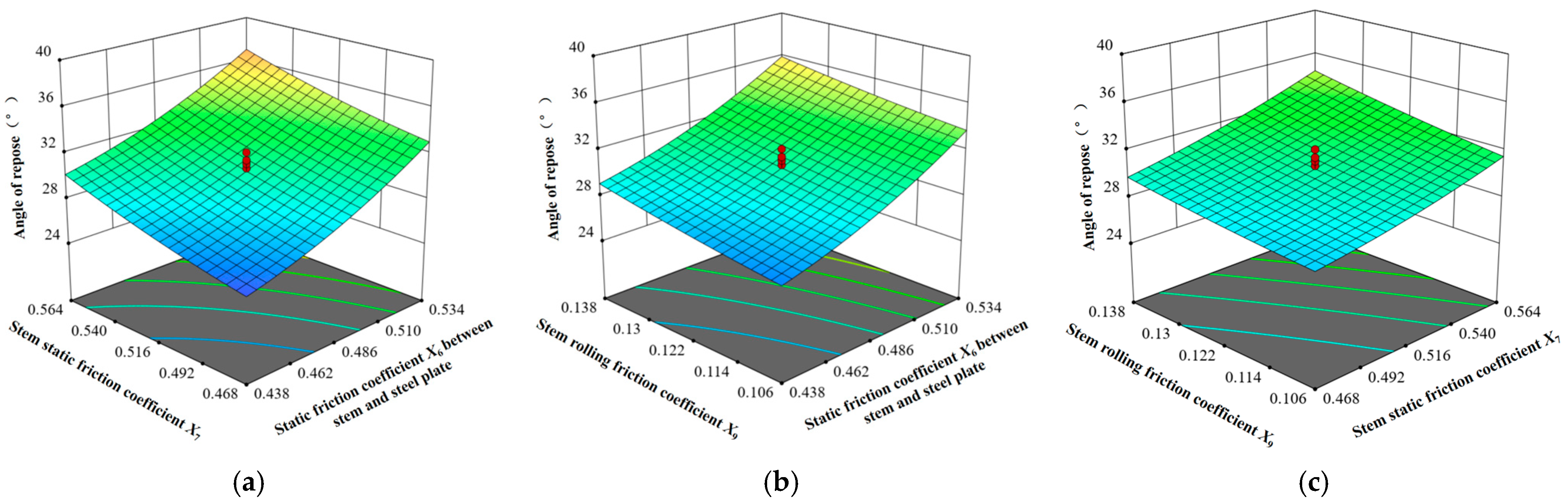
With the stem-stem RFC held constant, the RS for the stem-steel plate SFC and the stem-stem SFC is shown in Figure 8a. When the stem-steel plate SFC was held constant, the RA increased gradually with increasing stem-stem SFC. Similarly, when the stem-stem SFC was held constant, the RA increased gradually with increasing stem–steel plate SFC, indicating a significant trend in both cases.

With the stem-stem SFC held constant, the RS for the stem-steel plate SFC and the stem-stem RFC is shown in Figure 8b. When the stem-steel plate SFC was held constant, the RA increased gradually with increasing stem-stem RFC. When the stem-stem RFC was held constant, the RA increased gradually with increasing stem-steel plate SFC, and this trend was also significant.

With the stem-steel plate SFC held constant, the RS for the stem-stem SFC and the stem-stem RFC is shown in Figure 8c. When the stem-stem SFC was held constant, the RA increased gradually with increasing stem-stem RFC. When the stem-stem RFC was held constant, the RA increased gradually with increasing stem-stem SFC.

3.5. Comparative Analysis of Machine Learning Regression Models

To determine the most suitable regression model for subsequent experiments, the coefficient of determination (R²), mean squared error (MSE), and average absolute deviation (AAD) of the three regression model algorithms were compared [28,29,30,31]. For the BP neural network model, the number of neurons in the hidden layer was investigated using a trial-and-error method within the range of 3 to 13. Due to the limited number of training samples, prediction errors may occur during regression fitting. Therefore, the model was trained five times repeatedly, and the results are presented in

Table 8. Comparison of machine learning regression models.

Algorithm	Number of Hidden Layer Neurons	/	R2	AAD	MSE
SVR algorithm	/	Minimum	0.9258	0.7481	0.8986
		Maximum	0.9651	0.5867	0.4691
		Coefficient of variation	0.0209	0.1215	0.3103
BP algorithm	3	Minimum	0.8698	0.8839	1.2381
		Maximum	0.9029	0.7758	0.9874
		Coefficient of variation	0.0328	0.0657	0.1284
	4	Minimum	0.7839	1.5405	3.1076
		Maximum	0.8544	1.1156	1.8377
		Coefficient of variation	0.0609	0.2262	0.3631
	5	Minimum	0.5805	2.1752	6.1754
		Maximum	0.9057	0.8761	1.1898
		Coefficient of variation	0.1790	0.4077	0.7209
	6	Minimum	0.7395	1.6149	3.8338
		Maximum	0.9183	0.8278	0.9242
		Coefficient of variation	0.1234	0.4153	0.8227
	7	Minimum	0.5443	2.0855	6.3843
		Maximum	0.9228	0.6991	0.7341
		Coefficient of variation	0.2215	0.5144	0.9565
	8	Minimum	0.8574	1.6971	4.0968
		Maximum	0.9178	0.8383	1.1816
		Coefficient of variation	0.0236	0.2782	0.5824
	9	Minimum	0.7416	1.4307	3.6206
		Maximum	0.9444	0.7454	0.8190
		Coefficient of variation	0.3016	0.3782	0.8955
	10	Minimum	0.9052	1.1161	2.4355
		Maximum	0.9520	0.4775	0.4457
		Coefficient of variation	0.0284	0.3409	0.8013
	11	Minimum	0.8640	0.4904	0.3355
		Maximum	0.9344	0.2612	0.2629
		Coefficient of variation	0.0408	0.6038	0.9645
	12	Minimum	0.6617	1.6659	4.7395
		Maximum	0.8764	1.0214	1.7777
		Coefficient of variation	0.1391	0.2847	0.5754
	13	Minimum	0.8185	0.9785	1.7256
		Maximum	0.9262	0.9050	1.0858
		Coefficient of variation	0.0652	0.0736	0.2644
GA-BP algorithm	3	Minimum	0.8217	1.2645	2.3817
		Maximum	0.9286	0.7772	0.8829
		Coefficient of variation	0.0608	0.3125	0.7095
	4	Minimum	0.7921	1.9564	4.1014
		Maximum	0.9104	0.7690	0.3930
		Coefficient of variation	0.0779	0.8445	1.3595
	5	Minimum	0.8342	0.5952	0.8833
		Maximum	0.8833	0.5119	0.6766
		Coefficient of variation	0.0290	0.5155	1.2285
	6	Minimum	0.8458	1.5921	4.4316
		Maximum	0.9072	0.4855	0.2988
		Coefficient of variation	0.0359	0.6459	1.3419
	7	Minimum	0.8197	1.4996	2.6538
		Maximum	0.8972	0.6340	0.4508
		Coefficient of variation	0.0410	0.5817	1.0138
	8	Minimum	0.8881	2.0049	4.6842
		Maximum	0.9400	0.7177	0.7360
		Coefficient of variation	0.0469	0.7172	1.3616
	9	Minimum	0.8375	1.9693	4.6699
		Maximum	0.9419	0.3765	0.1870
		Coefficient of variation	0.2380	0.5496	0.8577
	10	Minimum	0.9020	0.5862	0.4298
		Maximum	0.9685	0.4163	0.2995
		Coefficient of variation	0.0393	0.1689	0.2662
	11	Minimum	0.7542	1.9127	4.5974
		Maximum	0.9428	0.6334	0.6202
		Coefficient of variation	0.1121	0.4850	0.7135
	12	Minimum	0.6420	1.5574	4.9892
		Maximum	0.9269	0.4274	0.2353
		Coefficient of variation	0.1834	0.5815	0.8116
	13	Minimum	0.8862	1.4761	3.2688
		Maximum	0.9511	0.7325	0.7200
		Coefficient of variation	0.0419	0.7170	0.6740

.

As shown in Table 8, a comprehensive analysis based on the three core evaluation metrics—coefficient of determination (R²), average absolute deviation (AAD), and mean squared error (MSE)—indicates that both the SVR model and the GA-BP model achieve higher prediction accuracy than the BP neural network. Among them, the SVR model exhibits the smallest coefficient of variation, indicating good fitting stability; however, its optimal metrics (R² = 0.9651, AAD = 0.5867, MSE = 0.4691) are still inferior to those of the GA-BP model with 10 hidden neurons. The GA-BP model with 10 hidden neurons simultaneously achieves the best performance among all compared algorithms, with the highest R² (0.9685), the smallest AAD (0.4163), and the smallest MSE (0.2995). Moreover, the coefficient of variation in this model remains at a low level, indicating that it not only possesses higher prediction accuracy but also exhibits good fitting stability and generalization ability.

The BP neural network suffers from random initialization of weights and thresholds, a tendency to fall into local optima, and large fluctuations in prediction results, resulting in low R² and high AAD and MSE, indicating insufficient nonlinear fitting capability. The GA-BP model integrates the global optimization capability of the genetic algorithm (GA) with the nonlinear mapping advantage of the BP neural network. By using GA to globally optimize the initial weights and thresholds of the BP network, it overcomes the drawbacks of slow convergence, premature convergence, and susceptibility to local optima, thereby improving the accuracy and reliability of the repose angle prediction model. In terms of both prediction accuracy and fitting stability, the GA-BP model with 10 hidden neurons performs best among the three algorithms.

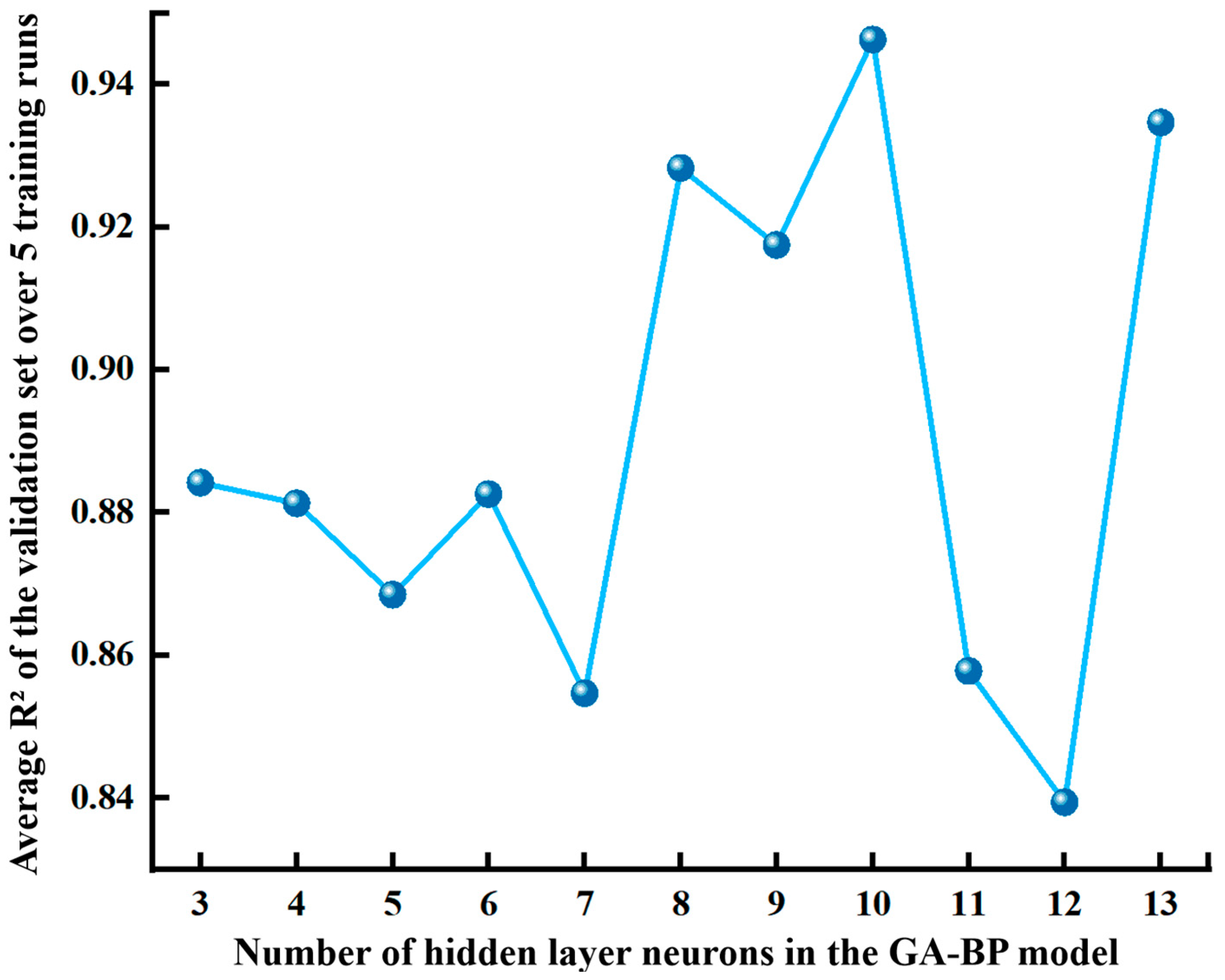
Furthermore, as shown in Figure 9, under five repeated training runs, the GA-BP model with 10 hidden neurons achieves the highest average R² on the validation set. Additionally, the variation trend of R² on the validation set for the GA-BP model is consistent with the R² results on the test set presented in Table 8, indicating that the model achieves simultaneous optimal performance on both validation and test sets, with no signs of overfitting or underfitting, and thus possesses reliable generalization ability. Based on the three aspects of fitting accuracy, stability, and generalization performance, the GA-BP model with 10 hidden neurons was ultimately selected as the optimal regression prediction model for calibrating the discrete element parameters of cassava seed stems. The topology structure of the GA-BP model was thus established, as shown in Figure 10.

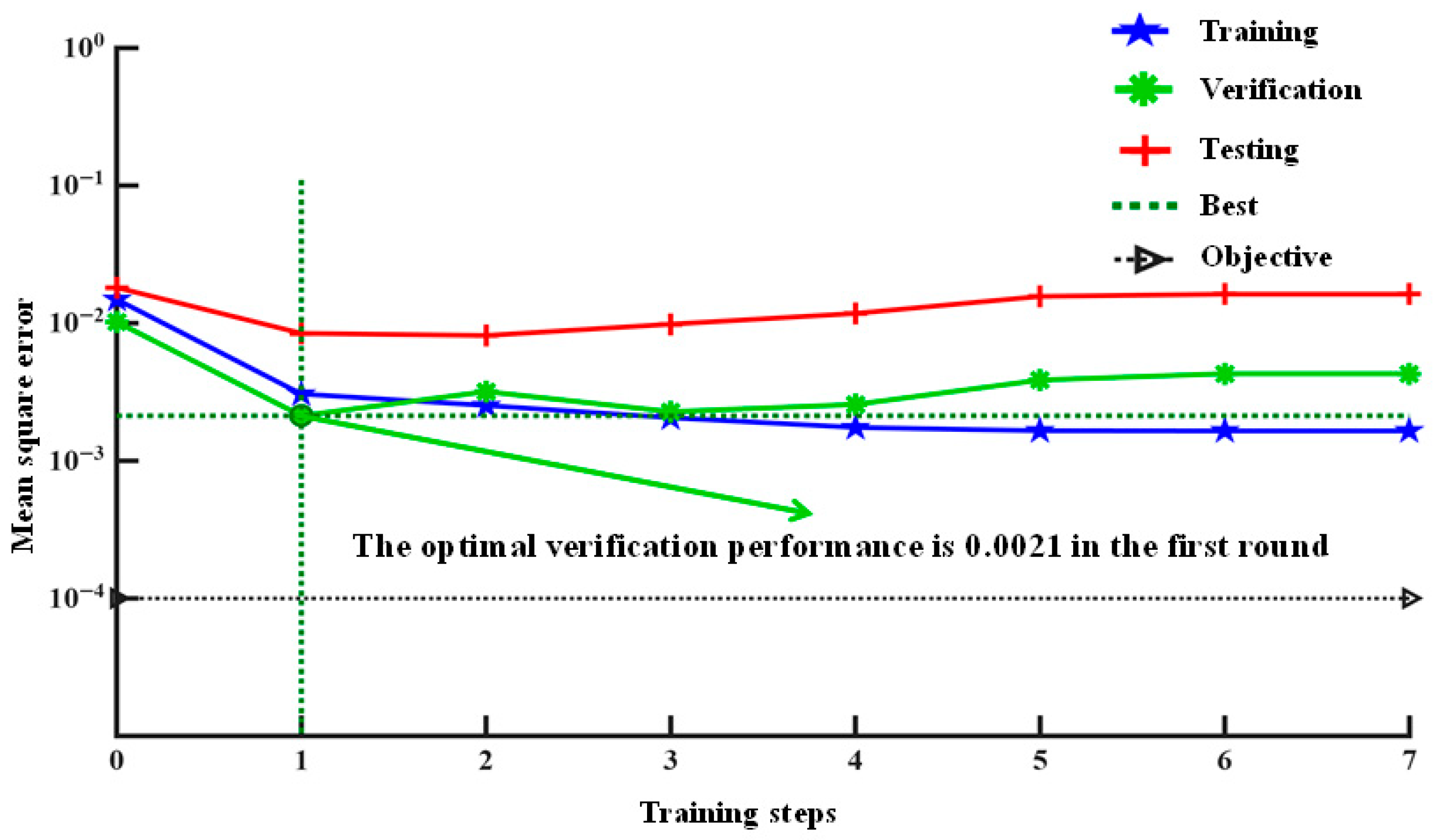
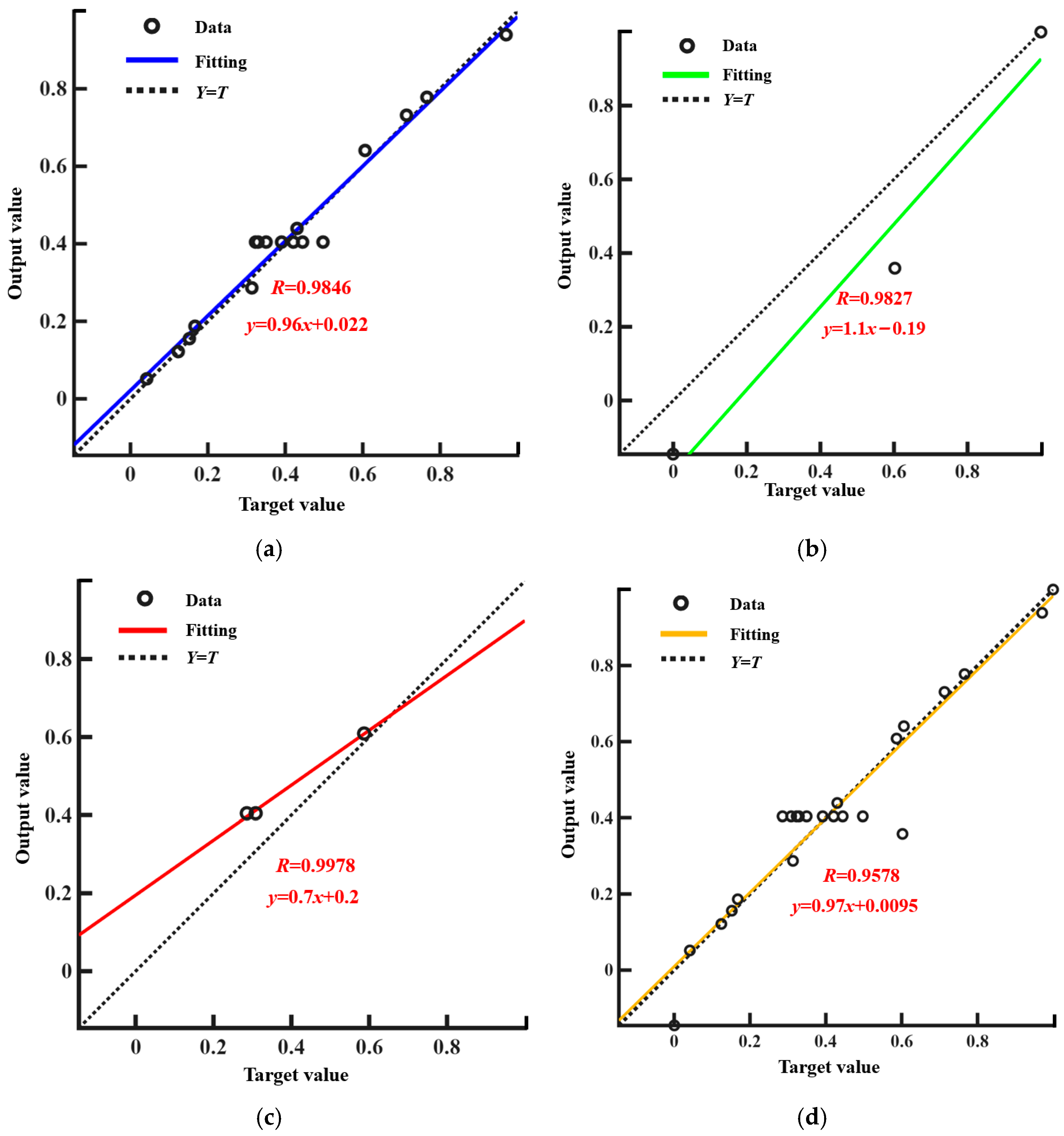
As shown in Figure 11, with increasing training epochs, the mean squared error (MSE) of the training, validation, and test sets was used for evaluation [31]; a smaller MSE indicated better accuracy of the model in describing the experimental results. The best validation performance was achieved at the first training step, with an MSE of 0.0021, indicating that the neural network training was completed. Based on this optimization, a neural network model with excellent performance was obtained. As shown in Figure 12, a good correlation was observed between the predicted and actual data.

3.6. Comparison Between RSM and GA-BP-GA Method

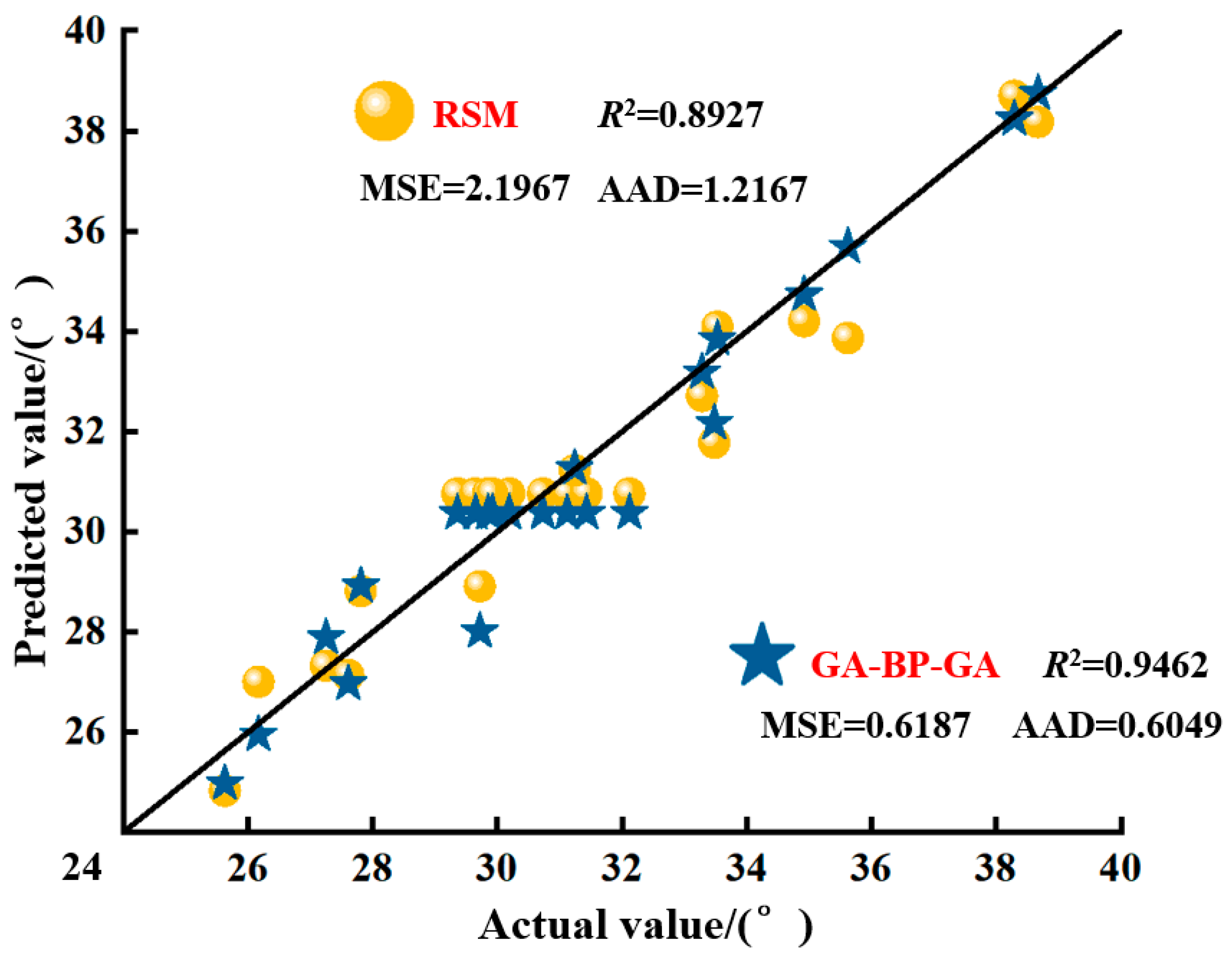
Figure 13 presents a comparison between the measured values and the predicted values of the two models, namely the RSM model and the GA-BP-GA model. From the overall trend, the predicted points of the GA-BP-GA model are more closely distributed around the diagonal, while those of the RSM model exhibit greater dispersion. In terms of prediction accuracy, the evaluation metrics of the GA-BP-GA model, AAD (0.6049) and MSE (0.6187), are significantly better than those of the RSM model (AAD = 1.2167, MSE = 2.1967), with AAD reduced by 50.28% and MSE reduced by 71.84%. This indicates that the GA-BP-GA model possesses higher prediction accuracy and lower error levels, enabling it to more accurately capture the complex nonlinear mapping relationship between the three significant contact parameters and the repose angle.

3.6.1. Parameter Optimization Using RSM

Using Design-Expert software, the average measured RA of the seed stems (30.28°) was set as the target, and the Numerical module was employed to optimize the regression model. The optimization constraints were set as follows:

$$\left\{\begin{array}{l}\theta =30.28°\\ \mathrm{s}.\mathrm{t}.\left\{\begin{array}{l}0.438\le X_6\le 0.534\\ 0.468\le X_7\le 0.564\\ 0.106\le X_9\le 0.138\end{array}\right.\end{array}\right.$$

(31)

Several sets of solutions were obtained, and the RA was validated through simulation. The optimal set of solutions, which exhibited a shape similar to that of the physical experiment, was determined as follows: the stem-steel plate SFC (X₆) was 0.492, the stem-stem SFC (X₇) was 0.469, and the stem-stem RFC (X₉) was 0.137. The simulated RA was measured to be 31.17°, with a relative error of 2.94% compared to the actual RA.

3.6.2. Parameter Optimization Based on the GA-BP-GA Method

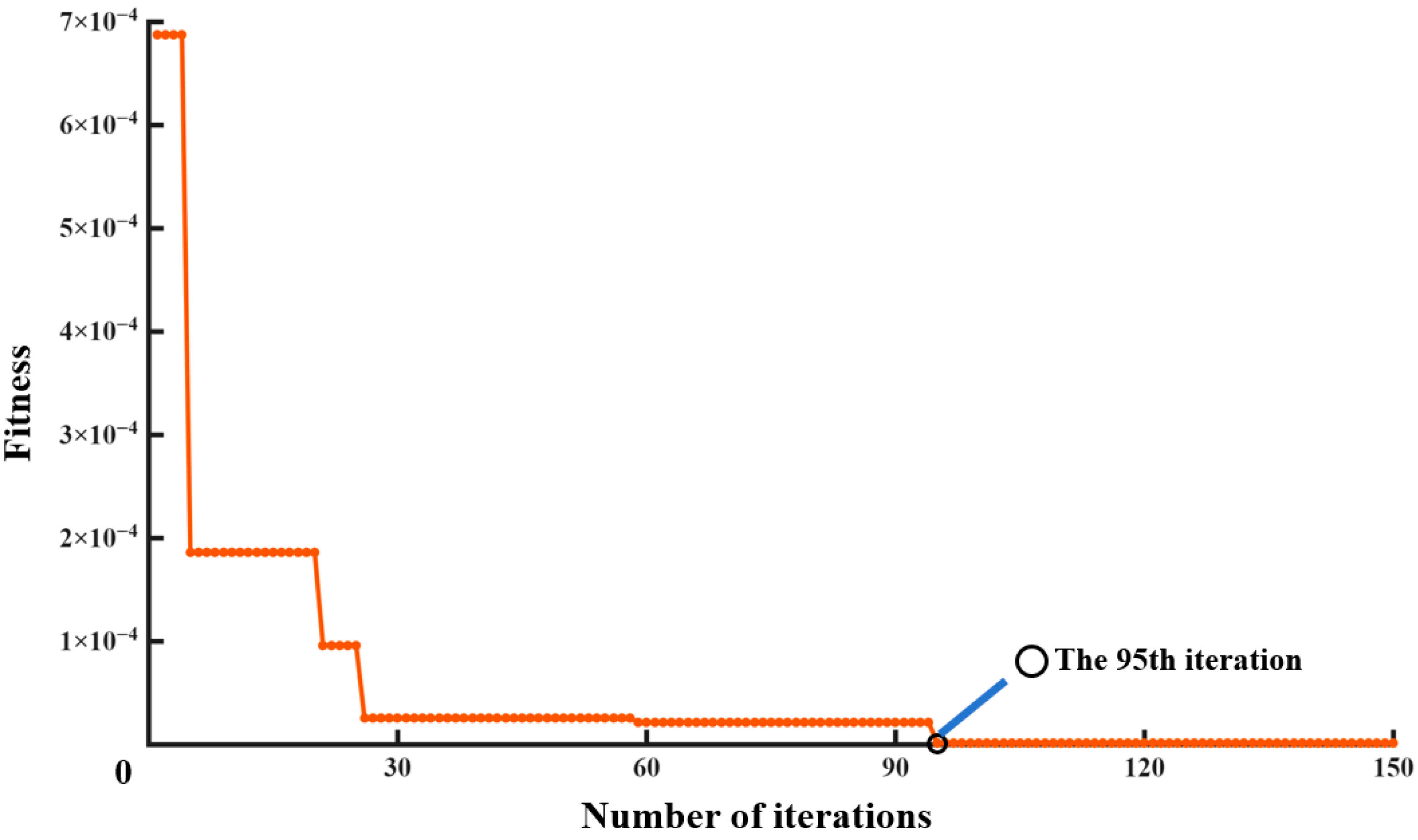
Figure 14 shows the fitness variation curve with evolutionary generation. Initially, the genetic algorithm (GA) utilized its population search characteristics, causing the fitness of selected individuals to decrease sharply. Subsequently, through multiple crossover and selection operations, the fitness of the selected individuals was fine-tuned within a small range, gradually approaching the target value [28,29,30,31]. The analysis indicated that by the 95th iteration, the fitness curve gradually converged to zero, suggesting that the difference between the predicted value and the target value was minimal. After multiple iterations, when the iteration count reached the target value of 150, the GA terminated the selection process and identified the individual with the closest fitness. Consequently, the optimal parameter combination obtained through optimization was a stem-steel plate SFC of 0.488, a stem-stem SFC of 0.489, and a stem-stem RFC of 0.131. Under this combination, the simulated RA was 30.73°, with a relative error of 1.49% compared to the actual RA. The prediction errors for the RA from both the RSM model and the GA-BP-GA model were less than 3%, indicating that the obtained optimal values for the three significant parameters were accurate, and both methods could be used for predicting the RA. The prediction accuracy of GA-BP was higher than that of the RSM, and the prediction error of the RA after GA-BP-GA optimization was smaller than that of the RSM, demonstrating that the prediction results of GA-BP-GA were closer to the actual values.

3.7. Validation Tests

3.7.1. RA Validation Test

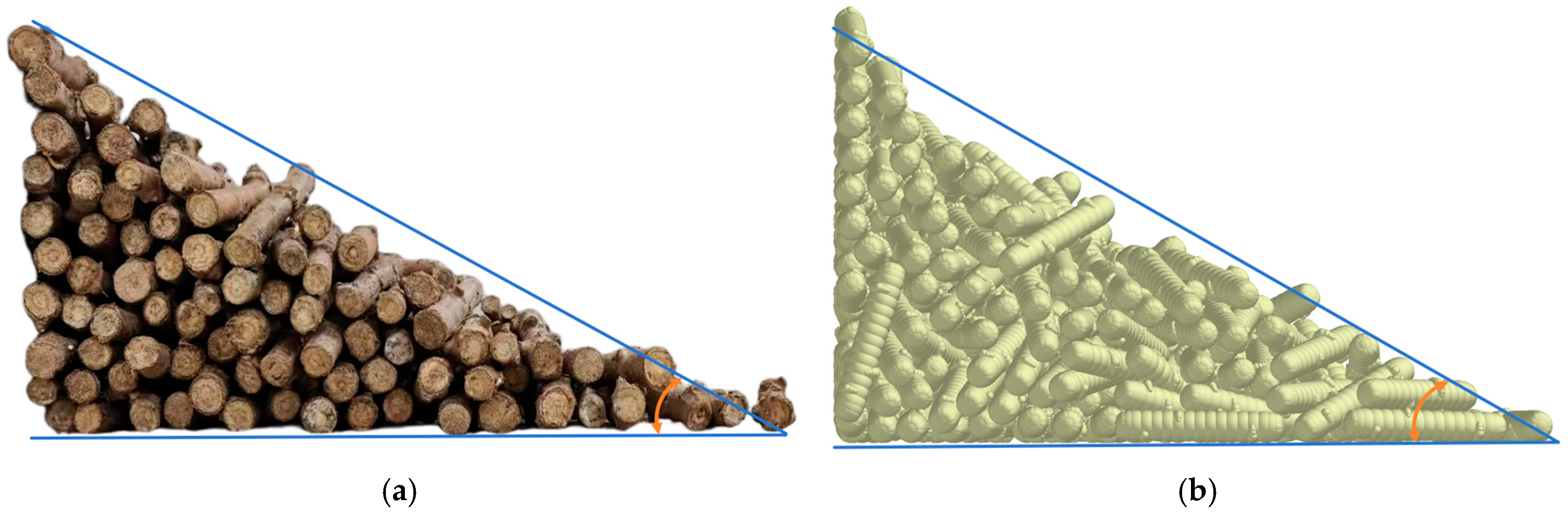
The parameter combination obtained from the optimization was validated through RA tests. As shown in Figure 15, the morphology of the seed stem pile from the simulation was close to that from the physical experiment. The simulated RA was 30.54°, while the experimental value was 29.93°. The relative error between the simulation and the experiment was 2.04%, indicating that the calibrated contact parameters were accurate and reliable, and could be used in subsequent collision damage tests of CSS using the Tavares model.

3.7.2. Collision Damage Test Using the Tavares Model

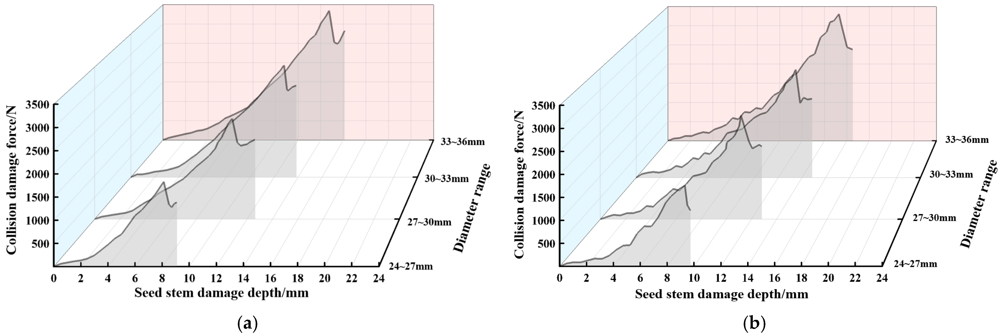
In the Tavares model, collision damage tests of seed stems can be conducted using the compression method [38,39] to obtain the pressure-displacement curves, collision damage force, and CDE of the seed stems. To ensure that the calibrated parameters are representative, four groups of seed stems with average diameters of 24–27 mm, 27–30 mm, 30–33 mm, and 33–36 mm were selected for the tests. Thirty seed stems with intact surfaces were selected from each group, and compression tests were performed on a computer-controlled electronic universal testing machine (WDW-50M) equipped with a 5 kN high-precision spoke-type load cell (accuracy ±0.5%) and a high-resolution displacement encoder, with a data acquisition frequency of 1000 Hz. During the test, the seed stem was placed horizontally at the center of the lower platen to ensure axial compression. The upper platen was loaded at a constant speed of 10 mm/min until macroscopic fracture of the seed stem occurred and the load dropped significantly, at which point the test was stopped. The system synchronously recorded the pressure-displacement data of the seed stem throughout the process for subsequent analysis. The results indicated that 81% of the seed stems were damaged in the axial direction, while 19% were damaged in the stem direction. The collision damage force and CDE varied among seed stems with different average diameters, indicating significant variability in the mechanical properties within the same material.

Based on the pressure-displacement curves of the seed stems, the CDE was obtained by integrating the section from the initial state to the peak damage force, and the specific CDE was further calculated using the following equation:

$$E_{11}={\displaystyle \frac{{\displaystyle {\int }_0^{s_b}{F}_{11}\mathrm{d}{s}_{11}}}{m_{11}}}$$

(32)

where $F_{11}$ is the collision damage force, N; $s_{11}$ is the damage depth of the seed stem, m; $s_b$ is the depth at which severe damage occurs, m; and $m_{11}$ is the mass of the seed stem, g.

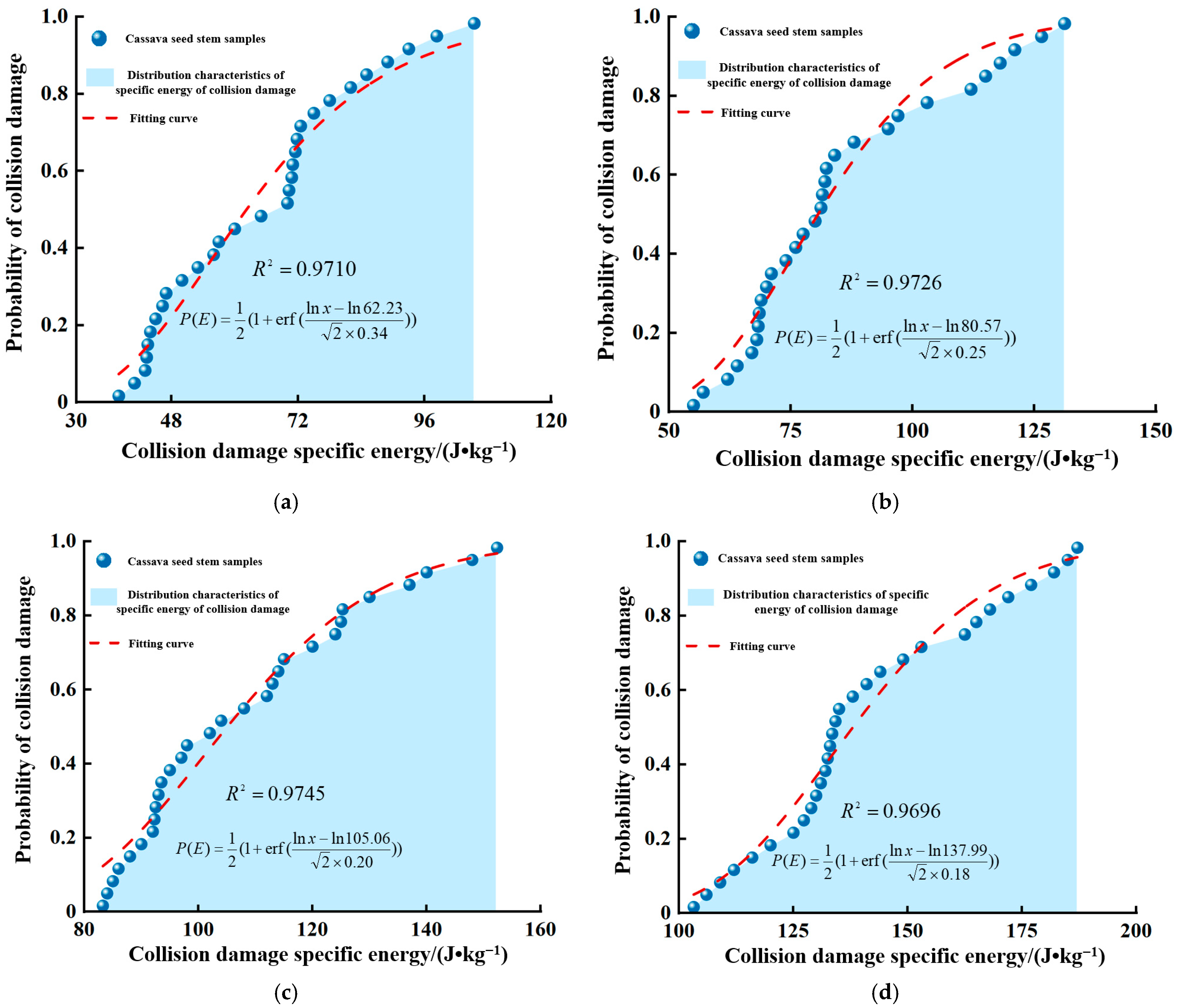
The data obtained from the system were imported into Origin software for integration to obtain the collision damage force of the seed stems in each test group. The specific CDE for each test group was calculated according to Equation (32), and the collision damage probability versus specific CDE curves [39] were plotted, as shown in Figure 16. The fitting results yielded median specific CDE values of 62.23, 80.57, 105.06, and 137.99 J/kg for the four groups of seed stems, with corresponding standard deviations of the log-normal distribution of 0.34, 0.25, 0.20, and 0.18, respectively. On this basis, the parameters of the Tavares model were further set, and the remaining parameters were obtained according to Equations (17)–(21), as presented in

Table 9. Tavares model breakage parameter settings.

γ	E∞/(J·kg−1)	d0/mm	σ	A	b	dmin/mm	Emin/(J·kg−1)
2.4	36.89	25.29	0.24	0.13	2.05	1	0.001

. Furthermore, the average values of collision damage force and CDE were statistically analyzed and compared with the experimental results to validate the Tavares collision damage model for seed stems. The variation pattern of collision damage force with damage depth for the seed stems is shown in Figure 17a, while Figure 17b presents the simulated variation pattern of collision damage force with damage depth, which exhibited good agreement with the experimental observations. Based on the variation pattern of collision damage force with damage depth, the collision damage force and CDE for the four diameter groups (24–27 mm, 27–30 mm, 30–33 mm, and 33–36 mm) were statistically analyzed, as shown in

Table 10. Results of the collision damage test for CSS.

Serial Number	Parameter
	Collision Damage Force/N	Collision Damage Energy/J
Test value for the 24–27 mm diameter group	1839.7	5.53
Simulated value for the 24–27 mm diameter group	1794.3	5.36
Relative error	2.47%	3.07%
Test value for the 27–30 mm diameter group	2339.6	8.38
Simulated value for the 27–30 mm diameter group	2385.5	8.23
Relative error	1.96%	1.79%
Test value for the 30–33 mm diameter group	2752.2	12.87
Simulated value for the 30–33 mm diameter group	2668.6	12.45
Relative error	3.04%	3.26%
Test value for the 33–36 mm diameter group	3428.9	17.06
Simulated value for the 33–36 mm diameter group	3286.2	16.68
Relative error	4.16%	2.23%
Average test value for the four diameter groups	2590.1	10.96
Average simulated for the four diameter groups	2533.6	10.68
Relative error	2.18%	2.55%

. The relative errors of collision damage force for the four groups were 2.47%, 1.96%, 3.04%, and 4.16%, respectively, and the relative errors of CDE were 3.07%, 1.79%, 3.26%, and 2.23%, respectively. All relative errors for all groups were less than 5%, and the average relative errors for the four groups were 2.18% (for collision damage force) and 2.55% (for CDE), both within 3%. These results indicate that the calibrated parameters of the Tavares model are accurate and can effectively describe the collision process of the seed stems.

4. Discussion

In this study, taking the “Guire No. 7” cassava seed stem (CSS) as the research object, the contact parameters and Tavares model breakage parameters were calibrated by combining physical experiments with discrete element (DE) simulations. The GA-BP-GA method was employed to achieve global optimization of the simulation parameters. The relative error of the calibrated simulation model for predicting the repose angle was 1.49%, and the relative errors for predicting the collision damage force and CDE were both less than 3%, thereby validating the effectiveness of the model.

4.1. Rationality Analysis of Calibrated Parameters

The contact parameters obtained by the GA-BP-GA method have clear physical meanings. The stem-steel plate SFC (0.488) and the stem-stem SFC (0.489) are both relatively high, mainly due to the rough epidermis and randomly distributed buds on the cassava seed stem, which generate mechanical interlocking upon contact and increase resistance to a certain extent. The stem-stem RFC (0.131) is also relatively high, attributed to the continuous obstruction of pure rolling by the protruding buds.

The collision damage force and CDE calibrated by the Tavares model reflect the response of cassava seed stems under axial compression. The xylem bears the majority of the load. As the load gradually increases, the pith reaches its limit and undergoes failure, eventually leading to overall damage of the seed stem. This process is consistent with the observed pattern of the experimental force-displacement curve (a linear increase, followed by a fluctuating plateau, and then a decline), thereby verifying the mechanical rationality of the calibrated parameters.

4.2. Practical Significance of the Research Findings for Precision Seeding Equipment Design

The calibrated contact parameters and the Tavares model provide quantitative simulation parameters for the design and performance optimization of cassava precision seeding equipment. The calibrated contact parameters can be used in discrete element simulations to simulate the flow and accumulation state of cassava seed stems inside the seed hopper. In the design of precision seeding equipment, blockage of the seed hopper outlet has long constrained operational efficiency and reliability. The stem-steel plate SFC (0.488) and stem-stem SFC (0.489) obtained in this study can serve as boundary conditions for discrete element simulations to evaluate the flow characteristics of cassava seed stems under different hopper inclination angles, wall materials, and surface treatment processes. When designing precision seeding equipment, simulations can predict the flow dead zones and accumulation patterns of cassava seed stems inside the hopper, thereby optimizing the hopper structural parameters, avoiding intermittent blockages during seed metering, and improving seeding continuity and uniformity.

The Tavares model provides a quantitative threshold for damage-prevention design of cassava seed stems. In the design of pre-cut seed metering devices and seed guide tubes, seed stems frequently collide with metal components and with each other during conveying. EDEM can be used to extract the collision energy distribution cloud map of seed stems during the metering process, identify high-collision-energy regions, and then optimize the material, inner wall roughness, and bending radius of the seed guide tube to ensure that the maximum collision energy along the conveying path remains below the damage threshold. This avoids latent mechanical damage to seed stems during mechanized seeding and improves bud integrity and germination rate.

4.3. Comprehensive Comparison Between RSM and GA-BP-GA Methods

In terms of computational efficiency, there are significant differences between RSM and GA-BP. RSM directly establishes a quadratic polynomial regression model based on a limited number of central composite design experiments without the need for iterative calculations, thus achieving relatively high computational efficiency. In contrast, the GA-BP method requires extensive iterative calculations. First, the BP neural network undergoes repeated training to fit the nonlinear mapping relationship, followed by multi-generational population evolution and optimization using a genetic algorithm [31]. Tang et al. [29] clearly pointed out that the GA-BP model is more time-consuming than RSM. However, this increase in computational cost is traded for higher prediction accuracy.

In terms of the practical application effectiveness of the parameter sets, the optimal parameter combinations obtained by the two methods often differ, leading to different results in subsequent secondary simulations or application-related simulations. Li et al. [31] found that the simulation error of the repose angle of silage optimized by RSM was 3.6%, whereas that optimized by GA-BP-GA was reduced to 1.3%, indicating that differences in parameter sets significantly affect simulation accuracy. Tang et al. [29] also noted that for the same geometric inputs, the deviation in separation efficiency prediction between RSM and GA-BP can exceed 2%, meaning that different methods may yield completely different optimal schemes in equipment design optimization. Ma et al. [30] further demonstrated that GA-BP reduced the average absolute error of the repose angle from 1.6678° (RSM) to 0.2677°, verifying the higher fidelity of the GA-BP parameter set in simulations. Therefore, when pursuing high-precision application simulations, the GA-BP method should be prioritized. Although its computational cost is higher, the resulting parameter set significantly improves the reliability of subsequent simulation outcomes.

4.4. Future Research Directions

In this study, moisture content was treated as a constant boundary condition (average value 62.73%). However, moisture content plays a decisive role in material adhesion, static friction coefficient, viscoelastic damping, and restitution coefficient. High moisture content increases surface adhesion and static friction coefficient, increases damping, and reduces the restitution coefficient. After moisture loss, seed stems become stiffer and more brittle. Because parameter calibration was not performed under multiple moisture content gradients, the quantitative effects of moisture on friction coefficients, restitution coefficients, stiffness, and damage energy remain unclear, limiting the applicability of the model under different moisture content conditions. Therefore, future research will investigate the influence of different moisture contents on the contact parameters and collision damage energy of seed stems to broaden the applicable operating range of the discrete element model. In addition, this study only used one variety (“Guire No. 7”), a single origin, and the same harvest period. Different varieties, planting regions, or maturity stages may all affect the discrete element parameters. The variation patterns of the calibrated parameters across different varieties, regions, or harvest stages have not been discussed, and the generalizability of the model to broader production conditions still requires validation. Therefore, future research will conduct comparative studies across multiple varieties, regions, and stages, selecting seed stems from different main production areas, representative varieties, and different harvest stages to analyze the differences in discrete element parameters caused by variety, planting region, and growth environment, thereby improving the model’s versatility and engineering applicability.

5. Conclusions

To address the limitation of discrete element method (DEM) simulations in studying the precision seeding mechanism and the damage and fracture mechanism of cassava seed stems (CSS) due to a lack of accurate parameters, this study focused on the “Guire No. 7” CSS and calibrated its discrete element (DE) parameters through a combination of physical experiments and DEM simulations. First, a non-spherical CSS model was constructed in EDEM to investigate the influence of different mesh face counts on model accuracy and simulation efficiency. The results showed that as the number of mesh faces increased, the volume relative error gradually decreased and stabilized, while the simulation time increased approximately linearly. Considering both accuracy and efficiency, the DE model with 15,790 mesh faces was selected for subsequent simulations, providing a methodological reference for the DE modeling of similar non-spherical stalk-type materials. Second, the Plackett–Burman design and the steepest ascent experiment were employed to screen the parameters that significantly affect the repose angle (RA) and to determine their optimal value ranges. Using the RA as the response value, a central composite design combined with three machine learning regression models (SVR, BP, and GA-BP) was applied to optimize the significant parameters and compare the methods. The results showed that the optimal parameters obtained through genetic algorithm optimization were a stem–steel plate static friction coefficient (SFC) of 0.488, a stem–stem SFC of 0.489, and a stem–stem rolling friction coefficient (RFC) of 0.131. The simulated RA was 30.73°, with a relative error of only 1.49% compared to the actual RA. The optimization performance of the GA-BP-GA method was superior to that of the central composite design method, demonstrating its better global optimization capability in handling strongly nonlinear parameter mappings. Third, the key parameters of the Tavares model were calibrated through physical experiments on seed stems, and the calibration was validated using collision damage force and CDE as indicators. The results showed that the relative errors between the experimental and simulated values of the average collision damage force and average CDE were both less than 3%, which is within the engineering allowable error range. This confirms the accuracy of the calibrated DE parameters for CSS and verifies the applicability of the Tavares model in simulating the energy collision damage behavior of CSS, thereby providing a reliable parameter foundation for subsequent simulation optimization of precision seeding machinery for cassava.

References

1. Yang, X.; Li, K.; Chen, S. Phenotypic Comprehensive Evaluation of Agronomic and Quality Characteristics of 30 Cassava Germplasm Resources. Mol. Plant Breed. 2022, 20, 6136–6144. [Google Scholar]
2. Chen, L.; Chen, R.; Atwa, M.E.; Li, H. Nutritional quality assessment of miscellaneous cassava tubers using principal component analysis and cluster analysis. Foods 2024, 13, 1861–1873. [Google Scholar] [CrossRef]
3. Borku, W.A.; Tora, T.T.; Masha, M. Cassava in focus: A comprehensive literature review, its production, processing landscape, and multi-dimensional benefits to society. Food Chem. Adv. 2025, 7, 100945. [Google Scholar] [CrossRef]
4. Afzia, N.; Ghosh, T. A comprehensive review on the fabrication of cassava peel-derived polysaccharides and their biocomposites for sustainable food packaging applications. Sustain. Food Technol. 2026, 4, 1394–1410. [Google Scholar] [CrossRef]
5. Hossain, M.D.; Yan, Q.; Zhou, Z.; Zhang, X.; Wittayakun, S.; Napasirth, V.; Napasirth, P.; Lukuyu, B.A.; Tan, Z. Cassava as a feedstuff for ruminant feeding system in Belt and Road countries: Innovations, benefits and challenges. J. Agric. Food Res. 2025, 21, 101874. [Google Scholar] [CrossRef]
6. Chen, L.; Xue, J.; Mou, X.; Ma, X.; Xiang, J. Design and experiments of the stepped vibration seed dispersal mechanism for pre-cut cassava planters. Trans. Chin. Soc. Agric. Eng. 2022, 38, 27–37. [Google Scholar]
7. Chen, L.; Lan, Y.; Dou, W.; Liu, Z.; Ma, X.; Chen, R. Finite element analysis of mechanical collision damage during precision seeding of cassava seed stems. J. South China Agric. Univ. 2024, 45, 427–436. [Google Scholar]
8. Yue, Y.; Zhang, Q.; Dong, B.; Li, J. Application of discrete element method to potato harvesting machinery: A review. Agriculture 2025, 15, 315. [Google Scholar] [CrossRef]
9. Zhao, H.; Huang, Y.; Liu, Z.; Liu, W.; Zheng, Z. Applications of discrete element method in the research of agricultural machinery: A review. Agriculture 2021, 11, 425–433. [Google Scholar] [CrossRef]
10. Li, Y.; Chen, Y.; Sun, X.; Lin, H.; He, J. Parameter calibration of the breakable flexible fiber model for maizestovers with different moisture contents. Trans. Chin. Soc. Agric. Eng. 2025, 41, 43–52. [Google Scholar]
11. Du, Z.; Li, D.H.; Li, X.P.; Jin, X.; Wu, Y.B.; Yu, F. Calibration and Experiment of Discrete Element Model Parameters for Tea Stem. Trans. Chin. Soc. Agric. Mach. 2025, 56, 311–320. [Google Scholar]
12. Li, Y.; Tian, X.; Zhao, Y.; Liu, X.; Zhou, M.; Dai, F.; Wang, W. Parameter calibration and experiment of polyhedral cottonseed discrete element model based on Tavares model. Trans. Chin. Soc. Agric. Mach. 2024, 55, 124–131. [Google Scholar]
13. Hu, Y.; Xiang, W.; Duan, Y.; Yan, B.; Ma, L.; Liu, J.; Lyu, J. Calibration of Ramie Stalk Contact Parameters Based on the Discrete Element Method. Agriculture 2023, 13, 1070. [Google Scholar] [CrossRef]
14. Wang, J.; Geng, B.; Yang, Z.; Yang, J.; Zhang, K.; Meng, Y. Discrete Meta-Modeling and Parameter Calibration of Harvested Alfalfa Stalks. Agronomy 2025, 15, 2390. [Google Scholar] [CrossRef]
15. Xu, C.; Xu, F.; Tang, H.; Wang, J. Determination of Characteristics and Establishment of Discrete Element Model for Whole Rice Plant. Agronomy 2023, 13, 2098. [Google Scholar] [CrossRef]
16. Han, D.; Zhang, H.; Liu, H.; Wang, C.; Wen, X.; Wang, X.; Chen, X.; Zhu, Y. Model construction and contact parameters calibration of dwarf-type plant stem based on DEM: The case of pod pepper stem. Comput. Part. Mech. 2025, 12, 3943–3964. [Google Scholar] [CrossRef]
17. Xu, T.; Gou, Y.; Huang, D.; Yu, J.; Li, C.; Wang, J. Modeling and Parameter Selection of the Corn Straw–Soil Composite Model Based on the DEM. Agriculture 2024, 14, 2075. [Google Scholar] [CrossRef]
18. Tavares, L.M.; Anderson, S.d.C. A stochastic particle replacement strategy for simulating breakage in DEM. Powder Technol. 2021, 377, 222–232. [Google Scholar] [CrossRef]
19. Shen, S.; Ji, S.; Zhao, D.; Han, Y.; Li, H.; Sun, Z.; Li, Z.; Li, A.; Feng, W.; Fei, J.; et al. Simulation of rice grain breakage process based on Tavares UFRJ model. Particuology 2024, 93, 65–74. [Google Scholar] [CrossRef]
20. Gabriel, A.C.; María, I.C.; Juliana, P. DEM breakage calibration for single particle fracture of maize kernels under a particle replacement approach. Chem. Eng. Res. Des. 2023, 195, 151–165. [Google Scholar] [CrossRef]
21. Chiaravalle, G.A.; Piña, J.; Cotabarren, M.I. DEM simulation of maize milling in a hammer mill. Powder Technol. 2025, 457, 120892. [Google Scholar] [CrossRef]
22. Bai, H.; Liu, F.; Dong, W. DEM modelling methods and trait analysis of sunflower seed. Biosyst. Eng. 2025, 250, 39–48. [Google Scholar]
23. Li, W.; Han, D.; Chen, P.; Qu, Z.; Dong, Q.; Chen, L.; Xu, L. Stratified DEM model construction and parameter optimization based on the cornstalk ontological traits. Results Eng. 2025, 27, 107081. [Google Scholar] [CrossRef]
24. Zhong, J.Q.; Tao, L.M.; Li, S.P.; Zhang, B.; Wang, J.Y.; He, Y.L. Determination and interpretation of parameters of double-bud sugarcane model based on discrete element. Comput. Electron. Agric. 2022, 203, 107428. [Google Scholar] [CrossRef]
25. Coetzee, C. Calibration of the discrete element method and the effect of particle shape. Powder Technol. 2016, 297, 50–70. [Google Scholar] [CrossRef]
26. Li, M.; Yu, Y.; Saxén, H. Computational study of the effect of friction coefficients and particle shape on the repose angle and porosity of sinter piles. Particuology 2025, 98, 231–240. [Google Scholar] [CrossRef]
27. Yu, W.; Liu, R.; Yang, W. Parameter Calibration of Pig Manure with Discrete Element Method Based on JKR Contact Model. AgriEngineering 2020, 2, 367–377. [Google Scholar] [CrossRef]
28. Niu, F.; Nie, Z.; Zhang, J.; Xing, Y.; Cao, Y.; Wang, X.; Shi, J.; Wu, J. Physically informed machine learning-enhanced DEM parameter calibration for cohesive wet coal. Powder Technol. 2026, 467, 121523. [Google Scholar] [CrossRef]
29. Tang, X.; Yue, Y.; Shen, Y. Prediction of separation efficiency in gas cyclones based on RSM and GA-BP: Effect of geometry designs. Powder Technol. 2023, 416, 118185. [Google Scholar] [CrossRef]
30. Ma, X.; Guo, M.; Tong, X.; Hou, Z.; Liu, H.; Ren, H. Calibration of Small-Grain Seed Parameters Based on a BP Neural Network: A Case Study with Red Clover Seeds. Agronomy 2023, 13, 2670. [Google Scholar] [CrossRef]
31. Li, G.; Ma, J.; Tian, X.; Zhao, C.; An, S.; Guo, R.; Feng, B.; Zhang, J. Discrete meta-simulation of silage based on RSM and GA-BP-GA optimization parameter calibration. Processes 2023, 11, 2784. [Google Scholar]
32. Diao, H.; Zeng, F.; Liu, Y.; Dou, M.; Zhang, Z.; Zhao, Z. Research on the Calibration of Discrete Elemental Parameters of Yam Bean Based on GA-BP Improved Neural Network Algorithm. Processes 2025, 13, 1537. [Google Scholar] [CrossRef]
33. Zeng, F.; Diao, H.; Liu, Y.; Ji, D.; Dou, M.; Cui, J.; Zhao, Z. Calibration and validation of simulation parameters for maize straw based on discrete element method and genetic algorithm–backpropagation. Sensors 2024, 24, 5217. [Google Scholar] [CrossRef] [PubMed]
34. Xia, H.; Deng, C.; Yang, T.; Huang, R.; Ou, J.; Dong, L.; Tao, D.; Qi, L. Development and Validation of a Discrete Element Simulation Model for Pressing Holes in Sowing Substrates. Agronomy 2025, 15, 971. [Google Scholar] [CrossRef]
35. Zhu, X.; Xu, Y.; Han, C.; Yang, B.; Luo, Y.; Qiu, S.; Huang, X.; Mao, H. Parameter calibration and experimental verification of the discrete element model of the edible sunflower seed. Agriculture 2025, 15, 292. [Google Scholar] [CrossRef]
36. Kong, L.; Du, J.; Yang, L.; Yao, X.; Hu, X.; Yin, H.; Tang, X. Rapid calibration of DEM parameters for corn straw–pig manure mixtures under variable moisture content for composting applications. Agriculture 2026, 6, 612. [Google Scholar] [CrossRef]
37. Yang, L.; Li, J.; Lai, Q.; Zhao, L.; Li, J.; Zeng, R.; Zhang, Z. Discrete element contact model and parameter calibration for clayey soil particles in the southwest hill and mountain region. J. Terramech. 2024, 111, 73–87. [Google Scholar] [CrossRef]
38. Zhou, Y.; Ji, Y. Simulation and experimental study of coarse coal breakage based on Tavares UFRJ model in pneumatic conveying. Powder Technol. 2025, 464, 121216–121222. [Google Scholar] [CrossRef]
39. Tino, A.A.; Barrios, K.G.; Tavares, M.L. Modeling iron ore breakage with the Tavares model and DEM simulation of a laboratory jaw crusher. Chem. Eng. Technol. 2025, 48, 139–152. [Google Scholar] [CrossRef]
Figure 1. Force analysis of CSS on a RFC measuring device.
Agriculture 16 01101 g001
Figure 2. Schematic diagram of measuring the collision recovery coefficient of CSS.
Agriculture 16 01101 g002
Figure 3. Schematic diagram of Tavares model.
Agriculture 16 01101 g003
Figure 4. Modeling of CSS with different number of fractal surfaces: (a) Mesh face count: 7922; (b) Mesh face count: 10,192; (c) Mesh face count: 13,870; (d) Mesh face count: 15,790; (e) Mesh face count: 17,678; (f) Mesh face count: 19,889; (g) Mesh face count: 22,164; (h) Mesh face count: 24,448; (i) Mesh face count: 27,158.
Agriculture 16 01101 g004
Figure 5. Volume relative error and simulation time of repose angle for CSS models with different numbers of mesh faces.
Agriculture 16 01101 g005
Figure 6. Extraction process of the simulated RA for CSS: (a) Seed stem pile formation process; (b) Original image of the seed stem RA; (c) Grayscale conversion of the image; (d) Image binarization; (e) Extraction of the RA contour; (f) Fitting of the seed stem RA; (g) Fitting of the seed stem RA.
Agriculture 16 01101 g006
Figure 7. Pareto Chart.
Agriculture 16 01101 g007
Figure 8. Laws of interaction factors on stacking angle: (a) RS for the stem-steel plate SFC and the stem-stem SFC with stem–stem RFC held constant; (b) RS for the stem-steel plate SFC and the stem-stem RFC with the stem-stem SFC held constant; (c) RS of the stem-stem SFC and the stem—stem RFC with the stem-steel plate SFC held constant.
Agriculture 16 01101 g008
Figure 9. Average R2 of validation set for GA-BP model with different hidden layer neurons over 5 training runs.
Agriculture 16 01101 g009
Figure 10. Topology structure of GA-BP model.
Agriculture 16 01101 g010
Figure 11. Performance curve.
Agriculture 16 01101 g011
Figure 12. Regression analysis results: (a) Training; (b) Verification; (c) Testing; (d) All.
Agriculture 16 01101 g012
Figure 13. Prediction and measured values of RSM and GA-BP-GA optimization method.
Agriculture 16 01101 g013
Figure 14. Fitness change curve.
Agriculture 16 01101 g014
Figure 15. Comparison of experimental and simulated stacking angles for cassava stem: (a) Test RA; (b) Simulated RA.
Agriculture 16 01101 g015
Figure 16. Probability of collision damage—specific energy curve of seed stem collision damage: (a) The average diameter of the CSS ranges from 24 to 27 mm; (b) The average diameter of the CSS ranges from 27 to 30 mm; (c) The average diameter of the CSS ranges from 30 to 33 mm; (d) The average diameter of the CSS ranges from 33 to 36 mm.
Agriculture 16 01101 g016
Figure 17. The variation pattern of cassava stem collision damage force with varying stem damage depth: (a) Test value; (b) Simulated value.
Agriculture 16 01101 g017