Agricultural Green Development as a Buffer Against Growing-Season Climate Extremes: Evidence from China’s Yellow River Basin

Abstract

Agricultural green development (AGD) is usually evaluated by its average productivity and environmental effects, but its value may be more visible when crop production is exposed to severe growing-season climate stress. This study examines whether AGD acts as a state-dependent buffer against climate-related output losses. Using a balanced panel of 56 prefecture-level cities in China’s Yellow River Basin from 2011 to 2024, we construct a Crop Extreme Stress Index (CESI) from daily meteorological records and estimate a two-stage least squares model with a crop-group shift-share instrument and crop-group price controls. The results show that AGD has a positive average association with crop output, but its marginal payoff is substantially larger in high-exposure years. In the preferred interaction specification, a one-standard-deviation increase in AGD is associated with approximately 2.8% higher crop output under high exposure. Quantile regressions further suggest that this protective effect is more visible in weaker output states. Channel consistency tests indicate that resilience capacity and crop diversification are more relevant under high exposure, although these results should not be interpreted as causal mediation. The findings suggest that AGD should be assessed not only by average productivity gains, but also by its capacity to reduce losses and stabilize output under growing-season climate extremes.

1. Introduction

Agricultural climate risk studies have often relied on annual mean temperature or precipitation to measure climate exposure [1]. These indicators are useful for capturing long-term climate trends, but they can miss short-duration extreme events that affect crop growth during sensitive phenological stages. For crop production, growing-season heatwaves, prolonged dry spells, and heavy precipitation can affect yields through heat stress, soil moisture deficits, waterlogging, erosion, and harvest disruption [2,3]. These shocks can cause substantial yield losses and increase output volatility [4,5]. Therefore, analyses of agricultural climate risk and adaptation should move beyond annual mean indicators and pay greater attention to the frequency, duration, and intensity of growing-season extremes [6,7]. This risk structure has important implications for how agricultural green development (AGD) should be evaluated. AGD refers to a production-oriented transition that seeks to improve agricultural performance while reducing resource consumption and environmental pressure [8,9]. Existing studies commonly measure AGD through green total factor productivity, eco-efficiency, carbon productivity, or composite evaluation systems that incorporate inputs, desirable outputs, and undesirable environmental outcomes [10,11]. However, this literature mainly evaluates whether AGD improves average productivity or environmental performance, and it provides less evidence on whether AGD reduces output losses under severe growing-season exposure [12]. If AGD has such a loss-reducing role, its value should be assessed not only through average efficiency gains but also through output stabilization under climate stress [13].

The first gap lies in the measurement of agricultural climate exposure. Annual temperature or precipitation anomalies are useful for studying long-term climate change, but they are often too coarse to capture event-based risks during the growing season. Prior research shows that crop responses to heat and water stress are strongly nonlinear. Even when annual averages change only slightly, daily-scale exposure can cause substantial losses once critical thresholds are exceeded. Moreover, extreme events often occur jointly rather than in isolation [7,14]. For example, high temperatures and drought may coincide within the same growing season and further amplify agricultural losses [15,16]. This suggests that climate exposure should be measured at the daily scale and should reflect both persistence and compounding across extreme-event dimensions. Existing studies have developed indicators for warm-period duration, consecutive dry days, and heavy precipitation intensity. The Expert Team on Climate Change Detection and Indices (ETCCDI) framework has become a widely used basis for monitoring climate extremes and supporting cross-regional comparison [17]. However, these daily-scale indicators have not been sufficiently incorporated into empirical research on AGD and agricultural resilience.

A second gap concerns how the value of AGD is evaluated. The AGD and sustainable agriculture literature has examined green productivity growth, eco-efficiency, carbon reduction, and the roles of environmental regulation, financial support, infrastructure, and technology adoption [18,19,20,21,22]. In measurement, data envelopment analysis (DEA)-based approaches are widely used to incorporate multiple inputs, desirable outputs, and undesirable environmental outputs. However, existing research provides limited evidence on whether AGD has a state-dependent return under extreme weather exposure [23]. Prior evidence suggests that some adaptation-related practices may have modest average effects but become more valuable in adverse years. This implies that a focus on mean outcomes may obscure the loss-mitigating role of AGD.

A third gap lies in empirical identification. AGD may evolve together with local policy support, infrastructure improvement, financial investment, and governance capacity, making simple correlations insufficient for causal interpretation [24]. Another source of bias arises when agricultural output is measured by output value. In disaster years, supply reductions may raise prices, so changes in reported output value may not accurately reflect actual production losses. As a result, apparent resilience may partly reflect valuation effects rather than genuine loss reduction. Therefore, the empirical design needs to address both AGD endogeneity and the price channel.

The Yellow River Basin provides a suitable setting for examining these issues [25]. It is an important agricultural region in China, but it also faces water scarcity, ecological fragility, and frequent compound weather shocks [26]. These conditions provide a relevant empirical setting for testing whether the return to AGD becomes larger when agricultural production faces high meteorological exposure [27,28].

Taken together, these limitations leave one central question unresolved: does AGD merely improve average agricultural performance, or does its marginal payoff become larger when crop production is exposed to severe growing-season climate extremes?

This study addresses these gaps in three ways. First, it constructs a Crop Extreme Stress Index (CESI) using daily meteorological data to capture growing-season exposure to heat, dry spells, and heavy precipitation. Second, it measures AGD using a slacks-based measure—global Malmquist–Luenberger (SBM–GML)—for the crop production system. Desirable output is defined by physical crop quantity rather than monetary value, which reduces mechanical overlap with value-based outcome variables. Third, it combines a crop-group shift-share instrumental-variable strategy with crop-group price controls to address both AGD endogeneity and the price channel. The analysis then tests whether the return to AGD is greater under high meteorological exposure, whether this pattern is more visible in weaker output states, and whether resilience capacity and crop diversification provide channel-consistent evidence.

The main contribution of this paper is to shift the evaluation of AGD from average productivity to state-dependent output stabilization [29]. By combining daily-scale exposure measurement, price-aware identification, quantile evidence, and channel consistency tests, the paper examines whether AGD is associated with downside protection under growing-season climate extremes. The channel evidence is interpreted as consistency evidence rather than as proof of a closed causal mediation mechanism.

2. Materials and Methods

This section presents the conceptual framework, study area, data sources, variable construction, empirical strategy, and implementation details. It explains how agricultural green development (AGD) is measured, how growing-season extreme exposure is constructed, how the high-exposure state is defined, and how the empirical models test whether the association between AGD and agricultural output varies across exposure states.

2.1. Conceptual Framework

This subsection formalizes the empirical prediction that the AGD–output association may vary across growing-season exposure states.

For crop production, severe exposure during the growing season may generate disproportionate output losses once heat, drought, or heavy precipitation exceeds agronomic tolerance thresholds. If AGD is associated with better production performance and lower sensitivity to such exposure, its marginal return should be larger in high-exposure years than in low-to-normal exposure years. This expectation does not imply a closed causal mechanism. It provides a testable empirical prediction: the association between AGD and output should vary across exposure states.

Observed agricultural output can be written as normal production performance net of climate-related losses:

$$Y_{it}^m = F^m(I_{it},{\mathrm{AGD}}_{it})-D^m({\mathrm{CESI}}_{it},{\mathrm{AGD}}_{it}) + {\mathit{\epsilon }}_{it}^m,m\in \left\{\mathrm{plant},\mathrm{total}\right\}$$

(1)

In Equation (1), $Y_{it}^m$ denotes outcome $m$ for city $i$ in year $t$. The superscript $\mathrm{p}\mathrm{l}\mathrm{a}\mathrm{n}\mathrm{t}$ refers to crop-planting output, and $\mathrm{t}\mathrm{o}\mathrm{t}\mathrm{a}\mathrm{l}$ refers to the broader agricultural output covering agriculture, forestry, animal husbandry, and fishery. $F^m(I_{it},\mathrm{A}\mathrm{G}{\mathrm{D}}_{it})$ denotes normal production performance, which depends on the input vector $I_{it}$ and $\mathrm{A}\mathrm{G}{\mathrm{D}}_{it}$. $D^m(E_{it},\mathrm{A}\mathrm{G}{\mathrm{D}}_{it})$ denotes output losses associated with growing-season extreme exposure. $E_{it}$ denotes the exposure state and is measured empirically by the Crop Extreme Stress Index (CESI). ${\epsilon }_{it}^m$ is the error term.

The loss function is assumed to increase with exposure and to be convex in exposure:

$${\displaystyle \frac{\mathsf{\partial }{D}^m(E_{it},\mathrm{A}\mathrm{G}{\mathrm{D}}_{it})}{\mathsf{\partial }{E}_{it}}}>0,{\displaystyle \frac{{\mathsf{\partial }}^2{D}^m(E_{it},\mathrm{A}\mathrm{G}{\mathrm{D}}_{it})}{\mathsf{\partial }{E}_{it}^2}}>0$$

(2)

Equation (2) means that climate-related losses increase as exposure rises and that marginal losses become larger under more severe exposure. If AGD reduces the sensitivity of losses to exposure, the cross-derivative of the loss function with respect to exposure and AGD should be negative:

$${\displaystyle \frac{{\mathsf{\partial }}^2{D}^m(E_{it},\mathrm{A}\mathrm{G}{\mathrm{D}}_{it})}{\mathsf{\partial }{E}_{it}\mathsf{\partial }\mathrm{A}\mathrm{G}{\mathrm{D}}_{it}}}<0$$

(3)

Because the loss term enters Equation (1) with a negative sign, Equation (3) implies that the marginal return to AGD should be larger when exposure is higher:

$${\displaystyle \frac{{\partial }^2{Y}_{it}^m}{\partial {\mathrm{AGD}}_{it}\partial {\mathrm{CESI}}_{it}}}> 0$$

(4)

Equation (4) provides the basis for the interaction specification. It implies that the marginal return to AGD should be larger when extreme exposure, measured by $\mathrm{C}\mathrm{E}\mathrm{S}{\mathrm{I}}_{it}$, is higher. In empirical terms, the coefficient on the interaction between AGD and the high-exposure indicator is expected to be positive.

The net marginal return can be written as:

$${∆}_{it}^m = {\displaystyle \frac{\partial Y_{it}^m}{\partial {\mathrm{AGD}}_{it}}}-\delta = {\displaystyle \frac{\mathsf{\partial }{F}^m(I_{it},\mathrm{A}\mathrm{G}{\mathrm{D}}_{it})}{\mathsf{\partial }\mathrm{A}\mathrm{G}{\mathrm{D}}_{it}}}-{\displaystyle \frac{\mathsf{\partial }{D}^m(E_{it},\mathrm{A}\mathrm{G}{\mathrm{D}}_{it})}{\mathsf{\partial }\mathrm{A}\mathrm{G}{\mathrm{D}}_{it}}}-\delta$$

(5)

In Equation (5), ${∆}_{it}^m$ denotes the net marginal return to AGD for outcome $m$, and $\mathit{\delta }\ge 0$ denotes adjustment costs associated with green production practices. The first derivative term captures the production performance component of AGD, whereas the second derivative term captures the loss reduction component. Under low exposure, adjustment costs may weaken the short-term net return. Under high exposure, the loss reduction component may become more visible.

A simplified empirical counterpart is the following interaction specification:

$$Y_{it}^m = {\mathit{\alpha }}_i +{ \mathit{\lambda }}_t + {\mathit{\beta }}_1^m{\mathrm{AGD}}_{it} + {\mathit{\beta }}_2^m({\mathrm{AGD}}_{it} \times {\mathrm{HighShock}}_{it})+X_{it}^{\prime }\theta +{\epsilon }_{it}^m$$

(6)

In Equation (6), ${\alpha }_i$ denotes city fixed effects, ${\lambda }_t$ denotes year fixed effects, $X_{it}$ is a vector of control variables, and $\mathrm{H}\mathrm{i}\mathrm{g}\mathrm{h}\mathrm{S}\mathrm{h}\mathrm{o}\mathrm{c}{\mathrm{k}}_{it}$ equals one when city $i$ in year $t$ belongs to the high-exposure state. The coefficient ${\beta }_1^m$ captures the marginal association between AGD and output in low-to-normal exposure years. The coefficient ${\beta }_2^m$ captures the additional marginal association under high exposure. A positive ${\beta }_2^{\mathrm{p}\mathrm{l}\mathrm{a}\mathrm{n}\mathrm{t}}$ would indicate that the AGD–output association is larger when crop production faces severe growing-season exposure.

This framework leads to three empirical expectations.

H1. 

State-dependent protection. The marginal payoff to AGD is larger under high growing-season exposure than under low-to-normal exposure.

H2. 

Downside protection. The protective effect of AGD under high exposure is more visible in lower-output states than in higher-output states.

H3. 

Greater channel relevance under high exposure. Resilience capacity and crop diversification are more strongly associated with output protection under high exposure than under low-to-normal exposure.

2.2. Study Area and Data Sources

This study uses a balanced panel of 56 prefecture-level cities in China’s Yellow River Basin from 2011 to 2024, yielding 784 city-year observations. The Yellow River Basin is selected because it is an important agricultural region and is simultaneously exposed to water scarcity, ecological fragility, and frequent growing-season climate extremes. These conditions provide a relevant empirical setting for testing whether the return to AGD becomes larger under high meteorological exposure.

The dataset combines meteorological, agricultural, environmental, and socioeconomic information. Daily meteorological data are obtained from the China Meteorological Data Service Center and the National Tibetan Plateau Scientific Data Center. These data are used to construct growing-season extreme exposure indicators from April to October. Agricultural, rural, and environmental statistics are collected from the China Agricultural Statistical Yearbook, China Rural Statistical Yearbook, and China Environment Statistical Yearbook. These yearbooks are used to construct agricultural output, input variables, AGD-related variables, environmental variables, control variables, and channel consistency variables.

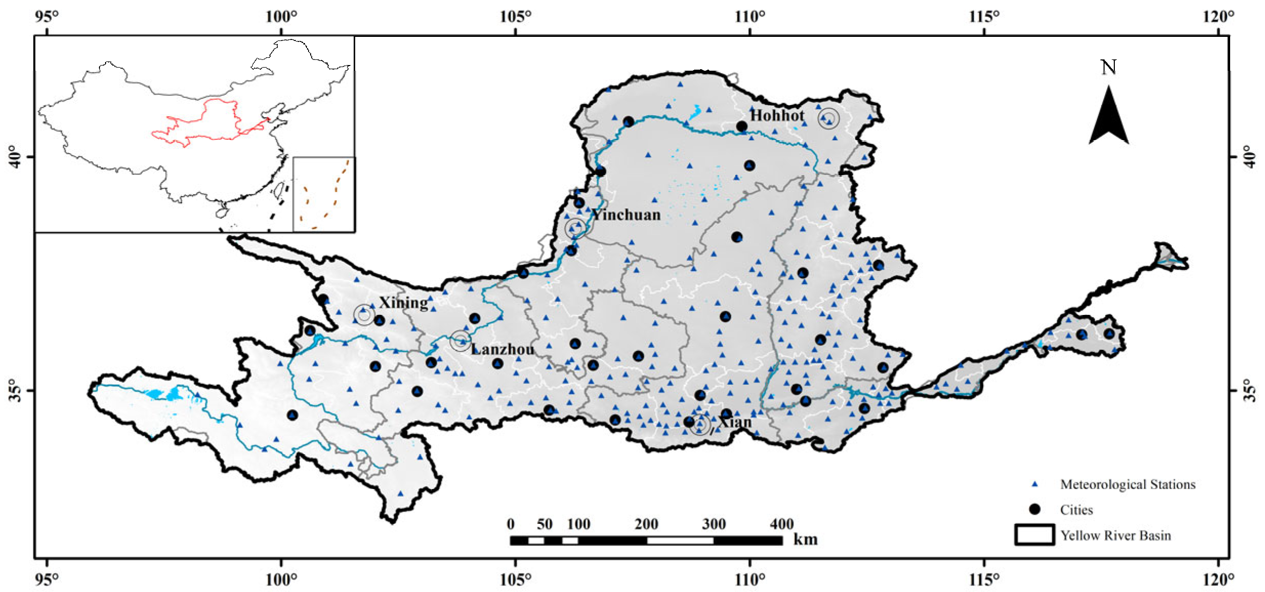
Several steps are taken to improve data consistency. Administrative boundary changes are harmonized to maintain comparable geographic units over time. Monetary variables are converted to constant 2011 prices using relevant price deflators. Continuous variables are winsorized at the 1st and 99th percentiles to reduce the influence of extreme outliers. Figure 1 presents the study area and the meteorological stations used to construct the daily-scale exposure indicators.

2.3. Variable Construction

2.3.1. Outcome Variables

The baseline outcome is planting-sector output, defined as the logarithm of the real gross output value of the crop-planting sector:

$$Y_{it}^{\mathrm{p}\mathrm{l}\mathrm{a}\mathrm{n}\mathrm{t}}=\ln ({\mathrm{Real} \mathrm{GOVA}}_{it}^{\mathrm{p}\mathrm{l}\mathrm{a}\mathrm{n}\mathrm{t}})$$

(7)

The extended outcome is total agricultural output:

$$Y_{it}^{\mathrm{t}\mathrm{o}\mathrm{t}\mathrm{a}\mathrm{l}}=\ln ({\mathrm{Real} \mathrm{GOVA}}_{it}^{\mathrm{t}\mathrm{o}\mathrm{t}\mathrm{a}\mathrm{l}})$$

(8)

In Equations (7) and (8), $\mathrm{R}\mathrm{e}\mathrm{a}\mathrm{l}\mathrm{G}\mathrm{O}\mathrm{V}{\mathrm{A}}_{it}^{\mathrm{p}\mathrm{l}\mathrm{a}\mathrm{n}\mathrm{t}}$ denotes the real gross output value of the crop-planting sector for city $i$ in year $t$, and $\mathrm{R}\mathrm{e}\mathrm{a}\mathrm{l}\mathrm{G}\mathrm{O}\mathrm{V}{\mathrm{A}}_{it}^{\mathrm{t}\mathrm{o}\mathrm{t}\mathrm{a}\mathrm{l}}$ denotes the real gross output value of agriculture, forestry, animal husbandry, and fishery. Both variables are measured at constant 2011 prices. Because the AGD index is constructed for the crop production system, $Y_{it}^{\mathrm{p}\mathrm{l}\mathrm{a}\mathrm{n}\mathrm{t}}$ is the main outcome. $Y_{it}^{\mathrm{t}\mathrm{o}\mathrm{t}\mathrm{a}\mathrm{l}}$ is used as supplementary evidence and should not be interpreted as a full-system AGD effect.

Value-based outcomes may be affected by price movements, especially in disaster years when supply reductions may raise crop prices [30,31]. To reduce this concern, the empirical models include crop-group price controls, and robustness checks use alternative outcomes, including agricultural value added and physical output.

2.3.2. Agricultural Green Development Index

The core explanatory variable is $\mathrm{A}\mathrm{G}{\mathrm{D}}_{it}$. In this study, AGD is understood as a production-system adjustment that improves agricultural performance while reducing resource use and environmental pressure. The empirical index mainly captures two dimensions: technical efficiency improvement and ecological pressure reduction [32]. Institutional and management conditions may support AGD, but they are not separately identified as independent components of the AGD index.

AGD is measured using a slacks-based measure—the global Malmquist–Luenberger (SBM–GML) index for the crop production system [33,34]. The index incorporates inputs, desirable outputs, and undesirable outputs. Inputs include land, labor, machinery, fertilizers, pesticides, plastic film, and irrigation. Desirable outputs are measured by physical crop quantities rather than monetary values. Crops are grouped into four categories: grain crops, oilseeds and cotton, vegetables and melons, and other cash crops [35].

Undesirable outputs include agricultural carbon emissions and agricultural non-point source pollution [36,37]. The desirable output vector is defined as:

$$Y_{it}^{+}=(Q_{1it},Q_{2it},Q_{3it},Q_{4it})$$

(9)

In Equation (9), $Q_{git}$ denotes the physical output of crop group $g$ in city $i$ and year $t$, where $g=1,\dots ,4$. Using physical crop quantities as desirable outputs helps reduce the mechanical link between the AGD index and value-based outcome variables. The same four crop groups are used in the AGD desirable output vector, crop diversification index, shift-share instrument, crop-group price controls, and alternative physical output aggregation. This keeps the variable construction internally consistent. The mathematical formulation of the SBM–GML index, including the directional distance function, global reference technology, undesirable output treatment, and variable units, is reported in Appendix B [38].

2.3.3. Growing-Season Extreme Exposure and Station-to-City Aggregation

Growing-season extreme exposure is constructed from daily meteorological records from April to October. This study focuses on three dimensions of exposure: persistent heat, prolonged dry spells, and heavy precipitation. These dimensions are measured using indicators from the Expert Team on Climate Change Detection and Indices (ETCCDI) framework: the warm spell duration index (WSDI), consecutive dry days (CDD), and total precipitation from very wet days (R95pTOT) [39,40]. The WSDI captures persistent heat exposure, CDD captures prolonged dry spells, and R95pTOT captures heavy precipitation. The threshold for each indicator is defined using the 1981–2010 reference period.

The indicators are first calculated at the station-year level and then aggregated to the city-year level. Because a single station may not fully represent city-level exposure, this study uses inverse distance weighting (IDW) to combine information from nearby stations [41]. Let $E_{st}$ denote a station-level extreme indicator for station $s$ in year $t$, and let $d_{is}$ denote the distance between city $i$ and station $s$. City-level exposure is calculated as:

$$E_{it}=\sum _{s\in S_i}{w}_{is}{E}_{st},w_{is}={\displaystyle \frac{d_{is}^{-2}}{\sum _{k\in S_i}{d}_{ik}^{-2}}}$$

(10)

In Equation (10), $S_i$ denotes the set of stations used for city $i$, and $w_{is}$ is the distance-based weight assigned to station $s$ for city $i$. IDW uses information from multiple nearby stations, preserves cross-city variation in exposure, and reduces measurement error caused by relying on a single station.

2.3.4. Construction of the Crop Extreme Stress Index and High-Exposure Indicator

The Crop Extreme Stress Index (CESI) summarizes multidimensional growing-season exposure. For each city-year observation, WSDI, CDD, and R95pTOT are standardized and then aggregated using principal component analysis (PCA). The CESI is defined as:

$${\mathrm{CESI}}_{it} = \mathrm{PC}1(z(\mathrm{W}\mathrm{S}\mathrm{D}{\mathrm{I}}_{it}),z(\mathrm{C}\mathrm{D}{\mathrm{D}}_{it}),z(\mathrm{R}95\mathrm{p}\mathrm{T}\mathrm{O}{\mathrm{T}}_{it}))$$

(11)

In Equation (11), $z(\mathrm{W}\mathrm{S}\mathrm{D}{\mathrm{I}}_{it})$, $z(\mathrm{C}\mathrm{D}{\mathrm{D}}_{it})$, and $z(\mathrm{R}95\mathrm{p}\mathrm{T}\mathrm{O}{\mathrm{T}}_{it})$ denote standardized city-level indicators, and $\mathrm{P}\mathrm{C}1(\cdot )$ denotes the first principal component. PCA is used because heat, dry spells, and heavy precipitation may occur jointly within the same growing season [14,15]. Entering the three indicators separately may increase multicollinearity and make exposure classification less stable. The purpose is to obtain a common growing-season exposure factor rather than to estimate the separate agronomic effect of each extreme-weather indicator. The direction of the index is normalized so that a higher CESI value indicates more severe exposure.

The CESI should be distinguished from the Agricultural Stress Index System (ASIS) developed by the Food and Agriculture Organization [42]. The ASIS is an operational monitoring and early-warning system mainly designed to identify agricultural areas exposed to drought or vegetation stress. The CESI serves a different purpose in this study. It is a city-year exposure index constructed for econometric analysis and combines daily weather-based indicators of persistent heat, dry spells, and heavy precipitation. Therefore, the ASIS and the CESI differ in data structure, hazard coverage, spatial-temporal unit, and research function.

The threshold $\widehat{\gamma }$ is estimated using a panel threshold model in which the AGD–output association is allowed to differ across CESI regimes [43]:

$$Y_{it}^{\mathrm{p}\mathrm{l}\mathrm{a}\mathrm{n}\mathrm{t}}={\mu }_i+{\lambda }_t+{\beta }_L\mathrm{A}\mathrm{G}{\mathrm{D}}_{it}\times 1(\mathrm{C}\mathrm{E}\mathrm{S}{\mathrm{I}}_{it}\le \gamma )+{\beta }_H\mathrm{A}\mathrm{G}{\mathrm{D}}_{it}\times 1(\mathrm{C}\mathrm{E}\mathrm{S}{\mathrm{I}}_{it}>\gamma )+X_{it}^{\prime }\theta +{\epsilon }_{it}$$

(12)

The threshold $\widehat{\gamma }$ is obtained by grid search and evaluated using bootstrap inference. This step is used only to define the exposure regime. The main state-dependent estimates are then obtained from the instrumental-variable specifications described in Section 2.4.

The high-exposure state is defined as:

$${\mathrm{HighShock}}_{it} = 1\left({\mathrm{CESI}}_{it} > \hat{\gamma }\right)$$

(13)

In Equation (13), $\widehat{\gamma }$ is the estimated threshold, and $1(\cdot )$ is an indicator function. A city-year observation is classified as high exposure when its CESI exceeds $\widehat{\gamma }$. This classification is based on meteorological exposure rather than realized crop losses, which helps avoid circularity between the exposure definition and the outcome variable.

2.3.5. Channel Consistency Variables and Controls

The channel examines whether the main result is consistent with observable buffering-related variables. It does not estimate a complete causal mediation mechanism. Two channel consistency variables are used: resilience capacity and crop diversification.

Resilience capacity, $\mathrm{A}\mathrm{C}\mathrm{R}\mathrm{c}\mathrm{a}{\mathrm{p}}_{it}$, captures local resources related to resistance, recovery, and adaptation. The baseline index is constructed from components related to water and irrigation capacity, drainage and flood-control capacity, insurance protection, fiscal buffer, human capital, information access, ecological buffering, and crop-system sensitivity [44]. To avoid mechanical overlap with the outcome variable, the index does not include actual crop output. A PCA-based index is used as a robustness check.

Crop diversification, $\mathrm{D}\mathrm{I}{\mathrm{V}}_{it}$, is measured using a Herfindahl-type index based on crop-area shares [45]:

$$\mathrm{D}\mathrm{I}{\mathrm{V}}_{it}=1-{\displaystyle \sum _{g=1}^4}{s}_{g,it}^2$$

(14)

In Equation (14), $s_{g,it}$ denotes the sown-area share of crop group $g$ in city $i$ and year $t$. A larger value indicates a more diversified crop structure. These two variables capture different dimensions of buffering capacity. Resilience capacity reflects local preparedness and response resources, whereas crop diversification reflects the production structure and its potential to spread risk [46]. Both are expected to be more strongly associated with output protection under high exposure.

The control variables include the logarithm of sown area, irrigation rate, road density, per capita GDP, urbanization rate, and non-agricultural employment. These variables control for production scale, agricultural infrastructure, economic development, urbanization, and labor allocation. Lagged controls are used in robustness checks to reduce simultaneity concerns.

2.4. Empirical Strategy

The empirical analysis proceeds in five steps. First, a two-way fixed-effects model describes the average association between AGD and agricultural output. Second, a two-stage least squares (2SLS) model estimates the average relationship using a crop-group shift-share instrument. Third, the preferred specification introduces the interaction between AGD and the high-exposure state to test whether the AGD–output association is larger under severe exposure. Fourth, panel quantile regressions examine whether the relationship is more visible in weaker output states. Fifth, channel consistency tests examine whether resilience capacity and crop diversification are more relevant under high exposure.

2.4.1. Baseline Two-Way Fixed-Effects Model

The baseline two-way fixed-effects model is specified as:

$$Y_{it}^{m }= {\mathit{\mu }}_i +{ \mathit{\lambda }}_t + {\beta }^m\mathrm{A}\mathrm{G}{\mathrm{D}}_{it}+X_{it}^{\prime }\theta +P_{it}^{\prime }\pi + {\epsilon }_{it}^m$$

(15)

In Equation (15), $Y_{it}^m$ denotes the outcome variable, $\mathrm{A}\mathrm{G}{\mathrm{D}}_{it}$ is the agricultural green development index, $X_{it}$ is a vector of control variables, and $P_{it}$ denotes crop-group price controls. City fixed effects ${\mu }_i$ absorb time-invariant city characteristics, while year fixed effects ${\lambda }_t$ absorb common shocks. ${\beta }^m$ captures the average association between AGD and outcome $m$.

2.4.2. Shift-Share Instrumental-Variable Strategy and Price Controls

AGD may be endogenous because it can co-evolve with local infrastructure, fiscal support, governance capacity, and development trends. To address this concern, this study uses a crop-group shift-share instrumental variable [47]:

$$Z_{it}={\displaystyle \sum _{g=1}^4}{s}_{i,g,2011}\cdot ∆\mathrm{A}\mathrm{G}{\mathrm{D}}_{-i,g,t}$$

(16)

In Equation (16), $s_{i,g,2011}$ is the baseline share of crop group $g$ in city $i$ in 2011, and $∆\mathrm{A}\mathrm{G}{\mathrm{D}}_{-i,g,t}$ denotes the national change in crop-group AGD in year $t$, constructed using a leave-one-out design that excludes city $i$. The identifying variation arises because cities with different initial crop structures are differently exposed to national crop-group AGD movements [48].

Because value-based output may be affected by crop prices, this study also includes crop-group price controls [31]:

$${\mathrm{PriceShock}}_{it}^{(g)} ={ \mathrm{s}}_{i,g,2011}·∆\ln P_{g,t},\hspace{1em}\hspace{1em}g =1,\dots ,4.$$

(17)

In Equation (17), $∆\ln P_{g,t}$ denotes the national log price change for crop group $g$. These price terms are included by crop group in both stages of the regression [30]. In the state-dependent specification, their interactions with $\mathrm{H}\mathrm{i}\mathrm{g}\mathrm{h}\mathrm{S}\mathrm{h}\mathrm{o}\mathrm{c}{\mathrm{k}}_{it}$ are also included to account for the possibility that price transmission differs in the high-exposure state.

The first-stage equation is:

$${\mathrm{AGD}}_{it} = {\mathit{\mu }}_i + {\mathit{\lambda }}_t + \pi Z_{it}+X_{it}^{\prime }\kappa +P_{it}^{\prime }\eta +{\nu }_{it}$$

(18)

The second-stage equation is:

$$Y_{it}^{m }= {\mathit{\mu }}_i + {\mathit{\lambda }}_t + {\beta }^m{\widehat{\mathrm{AGD}}}_{it} + X_{it}^{\prime }\theta +P_{it}^{\prime }\pi +{\epsilon }_{it}^m$$

(19)

The identifying assumption is that, conditional on city fixed effects, year fixed effects, controls, and crop-group price controls, the shift-share instrument affects local agricultural output only through local AGD. This assumption may be threatened if baseline crop structures are correlated with unobserved regional trends, or if national crop-group AGD shifts affect value-based output through crop prices rather than through local green production performance [49]. This study addresses these concerns in several ways. The national shifts are constructed using a leave-one-out design. Crop-group price controls are included in both stages [50]. Additional robustness checks add share-specific time trends and province-by-year fixed effects, use a purged-shifts instrument, and conduct off-season placebo and leave-one-crop-group-out tests [51]. These checks cannot directly prove the exclusion restriction, but they reduce the plausibility of the main alternative explanations.

2.4.3. State-Dependent 2SLS Specification

The preferred specification tests whether the AGD–output association is larger under high exposure:

$$Y_{it}^m={\mu }_i+{\lambda }_t+{\beta }_1^m\mathrm{A}\mathrm{G}{\mathrm{D}}_{it}+{\beta }_2^m(\mathrm{A}\mathrm{G}{\mathrm{D}}_{it}\times \mathrm{H}\mathrm{i}\mathrm{g}\mathrm{h}\mathrm{S}\mathrm{h}\mathrm{o}\mathrm{c}{\mathrm{k}}_{it})+\rho \mathrm{H}\mathrm{i}\mathrm{g}\mathrm{h}\mathrm{S}\mathrm{h}\mathrm{o}\mathrm{c}{\mathrm{k}}_{it}+X_{it}^{\prime }\theta +P_{it}^{\prime }\pi +(P_{it}\times \mathrm{H}\mathrm{i}\mathrm{g}\mathrm{h}\mathrm{S}\mathrm{h}\mathrm{o}\mathrm{c}{\mathrm{k}}_{it}{)}^{\prime }\omega +{\epsilon }_{it}^m$$

(20)

Equation (20) is the core state-dependent specification of this paper. It tests whether the marginal payoff to AGD increases in the high-exposure state. In the two-stage least squares implementation, both $\mathrm{A}\mathrm{G}{\mathrm{D}}_{it}$ and $\mathrm{A}\mathrm{G}{\mathrm{D}}_{it}\times \mathrm{H}\mathrm{i}\mathrm{g}\mathrm{h}\mathrm{S}\mathrm{h}\mathrm{o}\mathrm{c}{\mathrm{k}}_{it}$ are treated as endogenous. The instruments are $Z_{it}$ and $Z_{it}\times \mathrm{H}\mathrm{i}\mathrm{g}\mathrm{h}\mathrm{S}\mathrm{h}\mathrm{o}\mathrm{c}{\mathrm{k}}_{it}$. In practice, the first-stage system is estimated for both endogenous regressors using the same controls, fixed effects, and price terms as in the second-stage equation. The coefficient ${\beta }_1^m$ captures the marginal association between AGD and output in low-to-normal exposure years, while ${\beta }_2^m$ captures the additional marginal association under high exposure. The total marginal association under high exposure is ${\beta }_1^m+{\beta }_2^m$. The main expectation is ${\beta }_2^{\mathrm{p}\mathrm{l}\mathrm{a}\mathrm{n}\mathrm{t}}>0$. First-stage relevance and instrument strength are evaluated using Kleibergen–Paap and Sanderson–Windmeijer diagnostics, with detailed results reported in Appendix E.

2.4.4. Panel Quantile Regressions

To examine whether the AGD association is more visible in weaker output states, this study estimates panel quantile regressions [52]:

$${\mathrm{Q}}_{\mathit{\tau }}(Y_{it}^{\mathrm{plant}}\mid \cdot ) = {\mathit{\alpha }}_i(\mathit{\tau }) + {\mathit{\lambda }}_t(\mathit{\tau }) + {\mathit{\beta }}_1(\mathit{\tau }){\mathrm{AGD}}_{it} +{ \mathit{\beta }}_2(\mathit{\tau })({\mathrm{AGD}}_{it} \times {\mathrm{HighShock}}_{it}) +{ X}_{it}^{\prime }\theta (\mathit{\tau })+P_{it}^{\prime }\pi (\tau )$$

(21)

In Equation (21), $Q_{\tau }(Y_{it}^{\mathrm{p}\mathrm{l}\mathrm{a}\mathrm{n}\mathrm{t}}\mid \cdot )$ denotes the conditional quantile of crop-planting output at quantile $\tau$. The analysis is conducted for τ = 0.10, 0.25, 0.50, 0.75, and 0.90 [53]. If AGD is associated with downside protection, the interaction coefficient should be more visible at lower quantiles than at the upper tail of the output distribution.

2.4.5. Channel Consistency Tests

The channel consistency tests examine whether resilience capacity and crop diversification are more strongly associated with output under high exposure. They do not decompose the AGD effect into formal causal pathways. For each channel variable $M_{it}$, where $M_{it}\in \{\mathrm{A}\mathrm{C}\mathrm{R}\mathrm{c}\mathrm{a}{\mathrm{p}}_{it},\mathrm{D}\mathrm{I}{\mathrm{V}}_{it}\}$, the specification is [54]:

$$\begin{gathered} Y_{it}^{\mathrm{p}\mathrm{l}\mathrm{a}\mathrm{n}\mathrm{t}}={\mu }_i+{\lambda }_t+{\beta }_1\mathrm{A}\mathrm{G}{\mathrm{D}}_{it}+{\beta }_2(\mathrm{A}\mathrm{G}{\mathrm{D}}_{it}\times \mathrm{H}\mathrm{i}\mathrm{g}\mathrm{h}\mathrm{S}\mathrm{h}\mathrm{o}\mathrm{c}{\mathrm{k}}_{it})+\eta M_{it}+ \\ \varphi (M_{it}\times \mathrm{H}\mathrm{i}\mathrm{g}\mathrm{h}\mathrm{S}\mathrm{h}\mathrm{o}\mathrm{c}{\mathrm{k}}_{it})+X_{it}^{\prime }\theta +{\epsilon }_{it} \end{gathered}$$

(22)

In Equation (22), $\varphi$ indicates whether the channel variable is more strongly associated with output under high exposure. A positive $\varphi$ is interpreted as channel consistency evidence. If the coefficient on $\mathrm{A}\mathrm{G}{\mathrm{D}}_{it}\times \mathrm{H}\mathrm{i}\mathrm{g}\mathrm{h}\mathrm{S}\mathrm{h}\mathrm{o}\mathrm{c}{\mathrm{k}}_{it}$ decreases after adding the channel variable, the attenuation is treated as supplementary consistency evidence rather than as causal mediation [55].

2.5. Implementation and Inference

All baseline regressions include city and year fixed effects. Standard errors are clustered at the city level to allow arbitrary serial correlation within cities. The state-dependent specifications use nested bootstrap inference to incorporate the additional uncertainty introduced by threshold estimation and regime classification [43]. Continuous variables are transformed or standardized where appropriate, and monetary variables are measured at constant 2011 prices. The appendix reports technical details on the SBM–GML index, CESI diagnostics, threshold inference, IV construction, first-stage diagnostics, and robustness checks.

3. Results

This section reports the empirical results. The analysis first describes the main variables and then estimates the average relationship between AGD and crop output. It next defines the high-exposure state using the CESI threshold and tests whether the marginal payoff to AGD is larger under severe growing-season exposure. The section then examines whether the estimated payoff is more visible in weaker output states, whether the channel evidence is consistent with resilience capacity and crop diversification, and whether the results are robust to alternative identification and measurement choices.

3.1. Descriptive Statistics

Table 1. Descriptive statistics of main variables.

Variable	Mean	Std. Dev.	Min	Max
$Y^{\mathrm{p}\mathrm{l}\mathrm{a}\mathrm{n}\mathrm{t}}$	14.542	0.834	12.053	16.524
$Y^{\mathrm{t}\mathrm{o}\mathrm{t}\mathrm{a}\mathrm{l}}$	14.852	0.974	12.539	16.943
$\mathrm{A}\mathrm{G}\mathrm{D}$	1.019	0.083	0.851	1.249
$\mathrm{C}\mathrm{E}\mathrm{S}\mathrm{I}$	0.000	1.000	−2.534	3.585
$\mathrm{W}\mathrm{S}\mathrm{D}\mathrm{I}$ (days)	8.395	4.482	0.000	25.000
$\mathrm{C}\mathrm{D}\mathrm{D}$ (days)	28.000	12.000	10.000	65.000
$\mathrm{R}95\mathrm{p}\mathrm{T}\mathrm{O}\mathrm{T}$ (mm)	310.237	135.499	145.512	571.000
$\mathrm{H}\mathrm{i}\mathrm{g}\mathrm{h}\mathrm{S}\mathrm{h}\mathrm{o}\mathrm{c}\mathrm{k}$	0.277	0.447	0.000	1.000
$\mathrm{A}\mathrm{C}{\mathrm{R}}_{\mathrm{c}\mathrm{a}\mathrm{p}}$	0.434	0.121	0.134	0.701
$\mathrm{D}\mathrm{I}\mathrm{V}$	0.651	0.132	0.354	0.871
ln_sown_area	6.435	0.802	4.248	7.240
irrig_rate	0.596	0.184	0.274	0.891
road_density	1.375	0.525	0.425	3.660
ln_gdppc	11.051	0.573	9.524	12.25
urban_rate	0.563	0.132	0.370	0.860
nonfarm_share	0.815	0.069	0.684	0.904

Notes: The sample is a balanced panel of 56 prefecture-level cities in the Yellow River Basin from 2011 to 2024. Y^plant and Y^total are logarithms of real gross output values at constant 2011 prices. AGD = agricultural green development; CESI = Crop Extreme Stress Index; WSDI = warm spell duration index; CDD = consecutive dry days; R95pTOT = total precipitation from very wet days; HighShock = high-exposure indicator defined by 1(CESI_it > $\hat{\gamma }$); ACR_cap = Resilience Capacity Index; DIV = Crop Diversification Index. ln_sown_area, irrig_rate, road_density, ln_gdppc, urban_rate, and nonfarm_share denote the logarithm of sown area, effective irrigation rate, road density, logarithm of GDP per capita, urbanization rate, and non-agricultural employment share, respectively.

reports the descriptive statistics for the main variables. The sample is a balanced panel of 56 prefecture-level cities in China’s Yellow River Basin from 2011 to 2024, yielding 784 city-year observations.

The mean of $Y_{it}^{\mathrm{p}\mathrm{l}\mathrm{a}\mathrm{n}\mathrm{t}}$ is 14.542, with a standard deviation of 0.834. This indicates substantial variation in crop-planting output across cities and years. The mean of $Y_{it}^{\mathrm{t}\mathrm{o}\mathrm{t}\mathrm{a}\mathrm{l}}$ is 14.852, with a larger standard deviation of 0.974, reflecting the broader sectoral coverage of agriculture, forestry, animal husbandry, and fishery.

The AGD index has a mean of 1.019 and a standard deviation of 0.083, indicating variation in green production-system performance across the sample. CESI is standardized, with a mean of zero and a standard deviation of one. Its values range from −2.534 to 3.585, showing considerable heterogeneity in growing-season extreme exposure. The three CESI components also show meaningful variation. WSDI averages 8.395 days and reaches a maximum of 25 days. CDD averages 28.000 days and reaches a maximum of 65 days. R95pTOT averages 310.237 mm and reaches a maximum of 571.000 mm. These values indicate that the basin contains meaningful differences in persistent heat, prolonged dry spells, and heavy-precipitation exposure.

The regime indicator $\mathrm{H}\mathrm{i}\mathrm{g}\mathrm{h}\mathrm{S}\mathrm{h}\mathrm{o}\mathrm{c}{\mathrm{k}}_{it}$ has a mean of 0.277, indicating that 27.7% of city-year observations are classified as high exposure. This share suggests that high exposure is not limited to a small number of outlying observations. The channel variables also show variation. $\mathrm{A}\mathrm{C}\mathrm{R}\mathrm{c}\mathrm{a}{\mathrm{p}}_{it}$ has a mean of 0.434 and a standard deviation of 0.121, while $\mathrm{D}\mathrm{I}{\mathrm{V}}_{it}$ has a mean of 0.651 and a standard deviation of 0.132. Overall, the descriptive statistics provide sufficient variation in AGD, growing-season exposure, exposure states, and channel variables for the subsequent analysis.

3.2. Average Effects and Instrumental-Variable Benchmark

Table 2. Average effect of agricultural green development on crop output.

Variables	(1) TWFE	(2) 2SLS Baseline	(3) 2SLS + Price Shock Controls	(4) +Share × Time Trends	(5) + Prov × Year FE
Panel A: Second Stage (Dep var: $Y_{it}^{\mathrm{p}\mathrm{l}\mathrm{a}\mathrm{n}\mathrm{t}}$)
AGDit	0.211 *** (0.035)	0.239 *** (0.047)	0.249 *** (0.052)	0.326 *** (0.068)	0.268 *** (0.058)
Weather control (CESI)	Yes	Yes	Yes	Yes	Yes
price shock controls: 4 components	No	No	Both Stages	Both Stages	Both Stages
Share × time trends	No	No	No	Yes	No
Province × Year FE	No	No	No	No	Yes
Panel B: First Stage (Dep var: AGDit)
Zit (Shift-share IV)	—	0.436 *** (0.063)	0.412 *** (0.071)	0.385 *** (0.075)	0.395 *** (0.069)
Panel C: Diagnostics
Kleibergen–Paap rk Wald F	—	37.52	31.25	28.42	26.54
Anderson–Rubin p-value	—	0.047	0.032	0.018	0.025
Observations	784	784	784	784	784
City and Year FE	Yes	Yes	Yes	Yes	Prov × Year

Notes: The dependent variable is $Y_{it}^{\mathrm{p}\mathrm{l}\mathrm{a}\mathrm{n}\mathrm{t}}$. TWFE = two-way fixed effects; 2SLS = two-stage least squares; IV = instrumental variable; FE = fixed effects; KP = Kleibergen–Paap; AR = Anderson–Rubin. Columns (1)–(4) include city and year fixed effects; column (5) replaces year fixed effects with province-by-year fixed effects. The shift-share instrument is $Z_{it}$. Price shock controls are included in both stages in columns (3)–(5). Standard errors are clustered at the city level. *** denote significance at the 1% levels, respectively.

reports the average relationship between AGD and crop output across all years. This benchmark does not test state-dependent protection directly, but it shows whether AGD is associated with a positive average payoff.

The estimates show a positive and statistically significant relationship between AGD and crop output. The coefficients on AGD are positive and statistically significant across all five specifications. In economic terms, a one-standard-deviation increase in AGD is associated with an approximately 2–3% increase in average crop output. This magnitude indicates a moderate positive average payoff.

The estimate remains positive as additional identification and price channel controls are introduced. Column (1) reports the baseline two-way fixed-effects model. Column (2) introduces the shift-share instrumental variable. Column (3) adds price shock controls, and the AGD coefficient remains positive and similar in magnitude. Columns (4) and (5) add share-specific trends and province-by-year fixed effects, respectively, and the coefficient remains positive and statistically significant.

The first-stage results support instrument relevance in the average-effect specification. The shift-share instrument is positively associated with AGD across the IV specifications. The Kleibergen–Paap rk Wald F statistics support first-stage relevance, while the Anderson–Rubin tests provide weak-instrument-robust evidence that the estimated AGD effect is not driven by weak identification alone. Overall, Table 2 provides a positive average-effect benchmark for the state-dependent analysis. The next step is to test whether this payoff becomes larger under severe growing-season exposure.

3.3. CESI Threshold Estimation and High-Exposure Regime Definition

To test whether the payoff to AGD differs under severe exposure, the analysis first defines a regime based on meteorological exposure rather than on realized crop losses. The threshold model provides this definition by estimating a cutoff value for the CESI. Observations above that cutoff are classified as high exposure, whereas observations below it are classified as low-to-normal exposure.

Table 3. Threshold estimation for the Crop Extreme Stress Index and High-Exposure Regime Composition. (A) Threshold estimate and regime composition; (B) threshold existence test.

(A)
Item	Value
Threshold estimate $\hat{\gamma }$ (CESI)	0.849
Percentile of $\hat{\gamma }$ in CESI distribution	72.4th
High-exposure observations N (H = 1)	217
Low-to-normal exposure observations N (H = 0)	567
High-exposure share N (H = 1)/N	27.6%
Grid range for $\gamma$ search	15th–85th percentiles
Trimming rule (minimum regime share)	15%
Bootstrap replications	2000
95% bootstrap CI for $\gamma$	[0.715, 0.982]
(B)
Item	Value
Sup-LR statistic	45.32
Bootstrap p-value	0.005
Grid points/Trim/Bootstrap reps	400/0.15/2000

Notes: The threshold variable is CESI_it. The threshold $\widehat{\gamma }$ is estimated using a panel threshold model with city and year fixed effects. Sup-LR = supremum likelihood ratio statistic; CI = confidence interval. Bootstrap inference is used to test threshold existence and construct the confidence interval. $\mathrm{H}\mathrm{i}\mathrm{g}\mathrm{h}\mathrm{S}\mathrm{h}\mathrm{o}\mathrm{c}{\mathrm{k}}_{it}=1(\mathrm{C}\mathrm{E}\mathrm{S}{\mathrm{I}}_{it}>\widehat{\gamma })$. 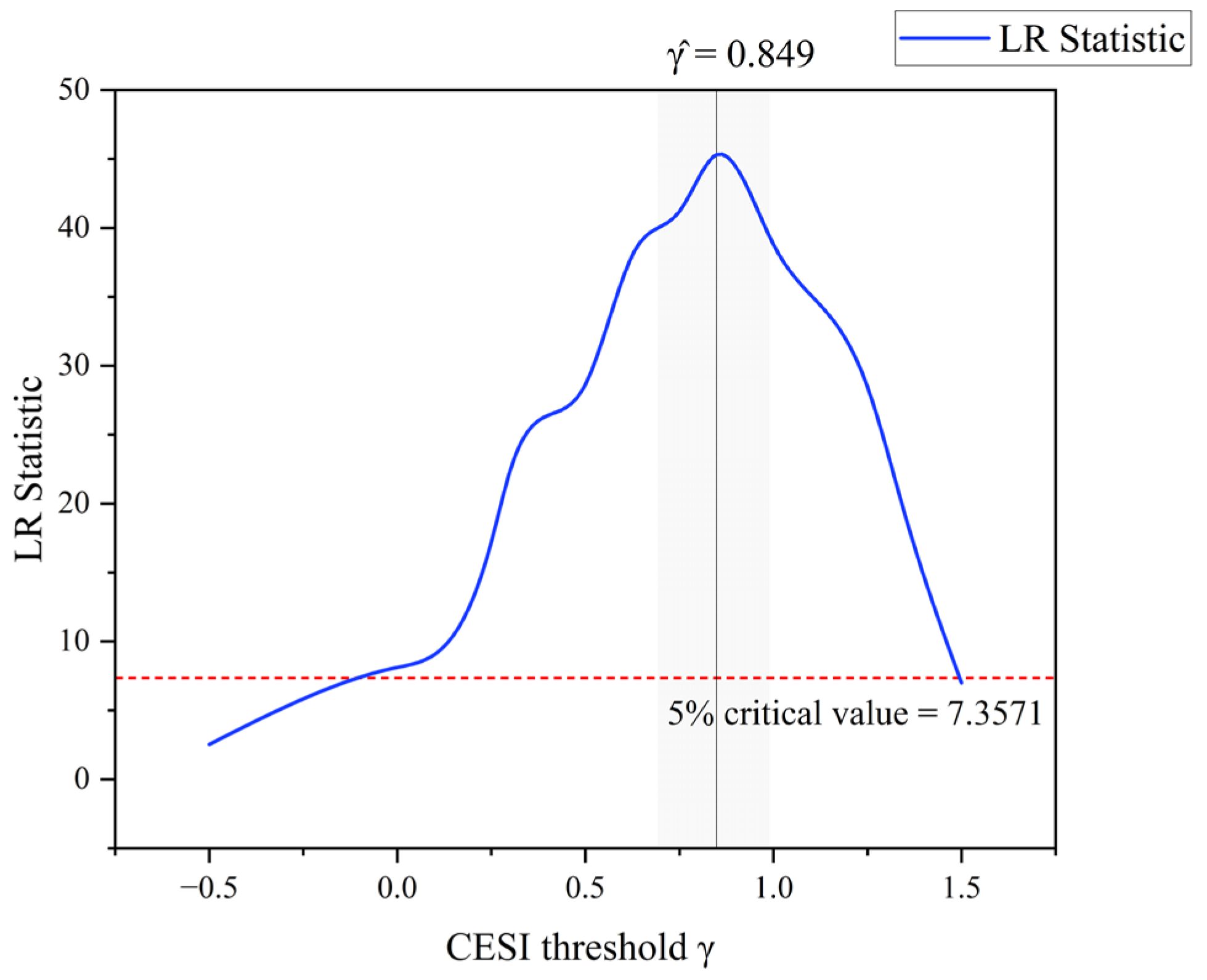Implementation details are reported in Appendix D.

reports an estimated CESI threshold of 0.849. This value lies at the 72.4th percentile of the CESI distribution, so the upper 27.6% of city-year observations are classified as high exposure. Among 784 city-year observations, 217 are classified as high exposure. This share indicates that high exposure represents a meaningful part of the sample rather than a small set of outliers.

The threshold is statistically supported. The sup-LR statistic rejects the null of no threshold, with a bootstrap p-value of 0.005. The estimated cutoff has a 95% bootstrap confidence interval ranging from 0.715 to 0.982. These results support the use of a data-driven high-exposure threshold.

Figure 2 visualizes the threshold estimation. The likelihood ratio statistic reaches its minimum around the estimated threshold of 0.849, with the confidence interval shown around the threshold estimate. This pattern supports the interpretation that the high-exposure states are data-driven rather than imposed mechanically [56].

This step provides an exposure-based way to classify observations before estimating the state-dependent AGD payoff. Because the regime is defined using the CESI rather than realized output losses, the subsequent comparison of AGD payoffs across exposure states avoids outcome-based classification.

3.4. State-Dependent Payoffs

Table 4. State-dependent effect of agricultural green development under high-exposure conditions.

Variables	(1) Interaction 2SLS	(2) + Price Shock Controls	(3) + Price × HighShock	(4) + Share × Time Trends
Panel A: Second Stage	Dep var: $Y_{it}^{\mathrm{p}\mathrm{l}\mathrm{a}\mathrm{n}\mathrm{t}}$
AGD (IV)	0.049	0.052	0.058	0.062
	[−0.052, 0.150]	[−0.045, 0.162]	[−0.038, 0.175]	[−0.032, 0.188]
AGD × HighShock (IV)	0.277	0.285	0.298	0.315
	[0.106, 0.524]	[0.115, 0.538]	[0.128, 0.552]	[0.145, 0.585]
High-exposure marginal effect	0.326	0.337	0.356	0.372
(β1 + β2)	[0.185, 0.513]	[0.198, 0.525]	[0.212, 0.548]	[0.235, 0.592]
Weather control (CESI)	Yes	Yes	Yes	Yes
Price controls: 4 components	No	Both Stages	Both Stages	Both Stages
Price × HighShock	No	No	Both Stages	Both Stages
Panel B: First-stage diagnostics (Sanderson–Windmeijer F; KP rk Wald F)
SW F for AGD	28.45	26.12	24.85	22.56
SW F for AGD × HighShock	22.18	20.45	19.32	18.15
KP rk Wald F	18.45	16.58	15.12	13.85

Notes: The dependent variable is $Y_{it}^{\mathrm{p}\mathrm{l}\mathrm{a}\mathrm{n}\mathrm{t}}$. AGD = agricultural green development; 2SLS = two-stage least squares; SW = Sanderson–Windmeijer; KP = Kleibergen–Paap. Both $\mathrm{A}\mathrm{G}{\mathrm{D}}_{it}$ and $\mathrm{A}\mathrm{G}{\mathrm{D}}_{it}\times \mathrm{H}\mathrm{i}\mathrm{g}\mathrm{h}\mathrm{S}\mathrm{h}\mathrm{o}\mathrm{c}{\mathrm{k}}_{it}$ are treated as endogenous and instrumented by $Z_{it}$ and $Z_{it}\times \mathrm{H}\mathrm{i}\mathrm{g}\mathrm{h}\mathrm{S}\mathrm{h}\mathrm{o}\mathrm{c}{\mathrm{k}}_{it}$, respectively. Weather controls include continuous $\mathrm{C}\mathrm{E}\mathrm{S}{\mathrm{I}}_{it}$. Price shock controls enter both stages in columns (2)–(4), and price-by-regime interactions enter both stages in columns (3)–(4). Brackets report 95% percentile confidence intervals from a city-clustered nested bootstrap. Each replication re-estimates the threshold, reconstructs $\mathrm{H}\mathrm{i}\mathrm{g}\mathrm{h}\mathrm{S}\mathrm{h}\mathrm{o}\mathrm{c}{\mathrm{k}}_{it}$, and re-estimates the 2SLS model.

tests whether the marginal payoff to AGD increases under severe growing-season exposure, which corresponds to H1. The model is a two-stage least squares specification in which both AGD_it and $\mathrm{A}\mathrm{G}{\mathrm{D}}_{it}\times \mathrm{H}\mathrm{i}\mathrm{g}\mathrm{h}\mathrm{S}\mathrm{h}\mathrm{o}\mathrm{c}{\mathrm{k}}_{it}$ are treated as endogenous and instrumented. The key quantities are ${\beta }_1$, which captures the marginal effect of AGD in the low-to-normal exposure years, ${\beta }_2$, which captures the additional effect in the high-exposure state, and ${\beta }_1+{\beta }_2$, which captures the total effect of AGD under high exposure.

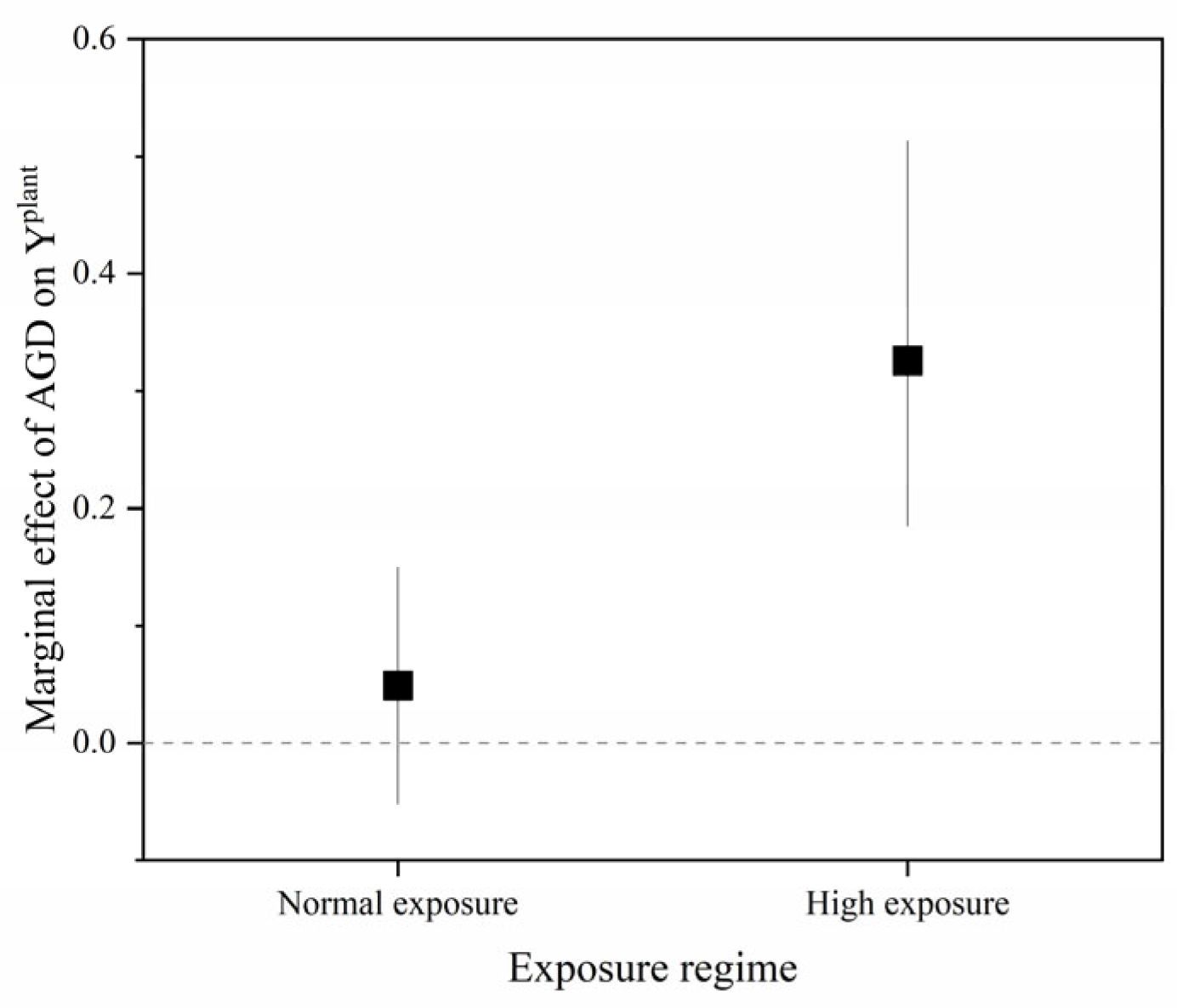
The estimate of ${\beta }_1$ is small and imprecisely estimated across specifications. In all four specifications, the coefficient on AGD alone is close to zero, and its confidence interval crosses zero. This indicates that the data do not provide strong evidence of a positive AGD payoff in the low-to-normal exposure state.

The interaction coefficient ${\beta }_2$ is positive across all specifications, and its bootstrap confidence interval does not include zero. This indicates that the marginal payoff to AGD is larger in the high-exposure state than in the low-to-normal exposure state. The estimate remains positive after adding price controls, price-by-regime interactions, and share-specific time trends.

The total marginal effect of AGD under high exposure is economically meaningful. Adding ${\beta }_1$ and ${\beta }_2$ yields a high exposure marginal effect ranging from 0.326 to 0.372 across the four specifications. Using column (2), a one-standard-deviation increase in AGD is associated with approximately 2.8% higher crop output under high exposure. This should not be interpreted as a uniform output premium in all years. Rather, it indicates that the payoff to AGD is concentrated in years when growing-season exposure is severe.

The Sanderson–Windmeijer and Kleibergen–Paap diagnostics indicate sufficient first-stage relevance for the endogenous regressors. These diagnostics reduce concerns about weak instrumentation in the state-dependent specifications.

Figure 3 presents the estimated marginal effects by exposure states. The marginal effect under low-to-normal exposure is close to zero, whereas the marginal effect under high exposure is positive and statistically distinguishable from zero. Taken together, Table 4 and Figure 3 support the state-dependent interpretation: the payoff to AGD is larger when growing-season exposure is severe.

3.5. Downside Protection: Distributional Evidence

Table 5. Quantile regression evidence on downside protection.

Variables	τ = 0.10	τ = 0.25	τ = 0.50	τ = 0.75	τ = 0.90
$\mathrm{A}\mathrm{G}\mathrm{D}$ (${\beta }_1$)	0.125 ** (0.063)	0.103 ** (0.042)	0.043 ** (0.017)	0.028 (0.018)	0.015 ** (0.006)
$\mathrm{A}\mathrm{G}\mathrm{D}\times \mathrm{H}\mathrm{i}\mathrm{g}\mathrm{h}\mathrm{S}\mathrm{h}\mathrm{o}\mathrm{c}\mathrm{k}$ (${\beta }_2$)	0.405 * (0.225)	0.230 ** (0.109)	0.182 *** (0.069)	0.342 ** (0.137)	0.052 ** (0.021)
High- exposure marginal effect	0.550 ** (0.213)	0.328 ** (0.159)	0.224 ** (0.104)	0.458 * (0.257)	0.067 * (0.039)
Controls	Yes	Yes	Yes	Yes	Yes
Observations	784	784	784	784	784

Notes: The dependent variable is $Y_{it}^{\mathrm{p}\mathrm{l}\mathrm{a}\mathrm{n}\mathrm{t}}$. Estimates are obtained using the Canay two-step fixed-effects quantile estimator. The specification includes $\mathrm{A}\mathrm{G}{\mathrm{D}}_{it}$, $\mathrm{A}\mathrm{G}{\mathrm{D}}_{it}\times \mathrm{H}\mathrm{i}\mathrm{g}\mathrm{h}\mathrm{S}\mathrm{h}\mathrm{o}\mathrm{c}{\mathrm{k}}_{it}$, controls, and fixed effects as described in the text. Standard errors in parentheses are obtained using a city-clustered bootstrap. The high-exposure marginal effect equals ${\beta }_1(\tau )+{\beta }_2(\tau )$. AGD = agricultural green development; HighShock = high-exposure indicator defined by the CESI threshold; CESI = Crop Extreme Stress Index. ***, **, and * denote significance at the 1%, 5%, and 10% levels, respectively.

examines whether the state-dependent AGD payoff differs across the crop output distribution. Rather than focusing only on the conditional mean, it tests whether the high-exposure payoff is more visible when output performance is weak. This is the downside-protection implication of the empirical framework.

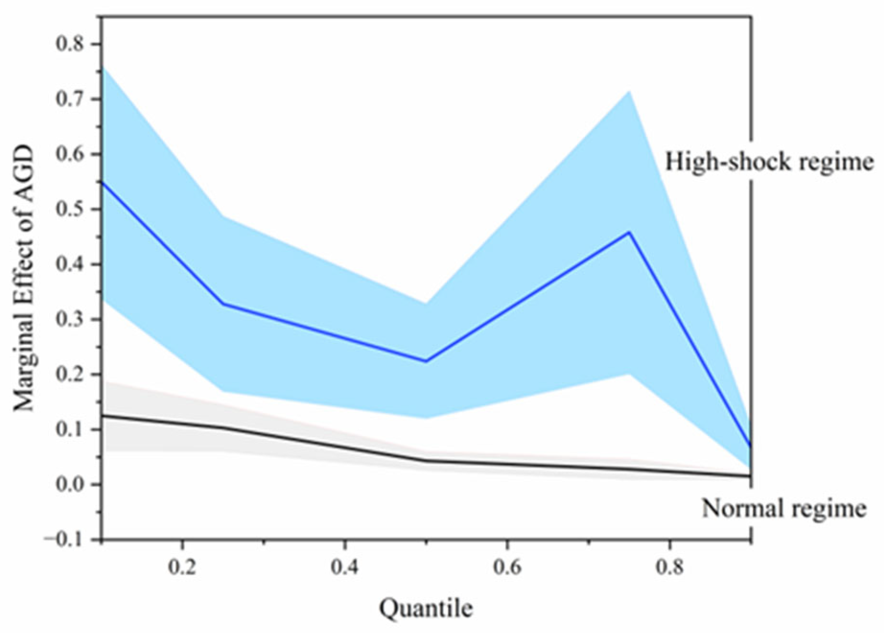
The estimates provide supportive, rather than perfectly monotonic, evidence of downside protection. The high-exposure marginal effect is largest at the 0.10 and 0.25 quantiles, indicating that AGD is particularly relevant when output performance is weak. The estimate at the 0.75 quantile is also relatively large, suggesting that the protective payoff is not confined exclusively to the lowest-output observations. However, the effect becomes much smaller at the 0.90 quantile.

The overall pattern is therefore best interpreted as evidence that AGD is more relevant in unfavorable or vulnerable output states, not as a strictly monotonic decline across the entire distribution. This interpretation is consistent with the loss reduction argument. If AGD is associated with reducing exposure-related losses, its return should be more visible when output is under pressure than when production conditions are already favorable.

Table 4 showed that the average high-exposure payoff is positive. Table 5 adds distributional evidence that this payoff is more closely related to weaker output states than to upper-tail output expansion. Figure 4 presents this distributional pattern.

3.6. Channel-Consistent Evidence

Table 6. Channel-consistent evidence for resilience capacity and crop diversification.

Panel A: Link with Channel Variables	(1) ACRcap (Capacity)	(2) DIV (Diversification)
AGD (IV)	0.245 *** (0.060)	0.193 ** (0.098)
Price-Channel Controls	Yes	Yes
Controls & Fixed Effects	Yes	Yes
Panel B: Outcome Relevance under High Exposure	(1) M = ACRcap	(2) M = DIV
AGD (IV)	0.044(0.036)	0.043 * (0.024)
AGD × HighShock (IV)	0.212 ** (0.098)	0.235 ** (0.113)
M (Channel Variable)	0.081 (0.053)	0.045 * (0.023)
M × HighShock (ϕ)	0.157 *** (0.048)	0.124 *** (0.035)
Panel C: Attenuation Diagnostic	(1) M = ACRcap	(2) M = DIV
$∆{\beta }_2$ (Attenuation %)	22.53%	15.79%
95% Bootstrap CI	[0.054, 0.391]	[0.033, 0.284]

Notes: Panel A reports 2SLS estimates linking instrumented AGD to the channel variables. Panel B reports output regressions including instrumented AGD, AGD × HighShock, the channel variable M, and M × HighShock. Panel C reports attenuation diagnostics as consistency checks, not as causal mediation. The attenuation share is calculated as (β2, baseline − β2, adjusted)/β2, baseline. Standard errors are reported in parentheses. AGD = Agricultural Green Development; ACRcap = Resilience Capacity Index; DIV = Crop Diversification Index; 2SLS = two-stage least squares; IV = instrumental variable. ***, **, and * denote significance at the 1%, 5%, and 10% levels, respectively.

reports channel consistency evidence for resilience capacity and crop diversification. Panel A examines whether instrumented AGD is associated with the two channel variables. Panel B examines whether these variables are more strongly associated with crop output under high exposure. Panel C reports attenuation diagnostics as supplementary consistency checks.

Panel A shows that AGD is positively associated with both channel variables. The coefficient on AGD is 0.245 in the resilience-capacity equation and 0.193 in the diversification equation. Panel B shows that the interaction terms between the channel variables and HighShock are positive and statistically significant. The interaction coefficient is 0.157 for resilience capacity and 0.124 for crop diversification, indicating that both variables are more strongly associated with crop output under high exposure.

Panel C shows that the coefficient on AGD × HighShock declines after adding the channel variables and their interactions. Relative to the baseline interaction coefficient of 0.298, the coefficient declines to 0.231 after adding resilience capacity and to 0.251 after adding crop diversification. These changes correspond to attenuation shares of 22.53% and 15.79%, respectively. This pattern is consistent with the channel interpretation, but it should not be read as a causal mediation decomposition.

3.7. Robustness Checks

Table 7. Robustness checks for the state-dependent payoff.

Panel A: Price-Channel Control Variants	(1) 4-Component PriceShock	(2) 4-Component × HighShock
AGD × HighShock (β2)	0.285	0.298
Bootstrap 95% CI	[0.115, 0.538]	[0.128, 0.552]
Panel B: Trend & FE Robustness	(1) Share× Linear Trend	(2) Province × Year FE
AGD × HighShock (β2)	0.315	0.302
Bootstrap 95% CI	[0.145, 0.585]	[0.132, 0.565]
Panel C: Purged Shifts Instrument	(1) Instrumented with Zit (Residual-based)
AGD × HighShock (β2)	0.279
Bootstrap 95% CI	[0.110, 0.525]
Panel D: Quantity-Based Outcomes	(1) Y = ln(GEO) (Physical)	(2) Y = ln(GrainOutput)
AGD × HighShock (β2)	0.192	0.175
Bootstrap 95% CI	[0.045, 0.371]	[0.038, 0.355]
Panel E: Methodological Sensitivity	(1) Alternative CESI	(2) Drop 2021 (Floods)
AGD × HighShock (β2)	0.264	0.275
Bootstrap 95% CI	[0.105, 0.422]	[0.120, 0.429]

Notes: Each panel reports the coefficient on $\mathrm{A}\mathrm{G}{\mathrm{D}}_{it}\times \mathrm{H}\mathrm{i}\mathrm{g}\mathrm{h}\mathrm{S}\mathrm{h}\mathrm{o}\mathrm{c}{\mathrm{k}}_{it}$ from the interaction 2SLS specification, with 95% confidence intervals. Panel A varies the price-channel control design. Panel B adds share-specific time trends and province-by-year fixed effects. Panel C uses a purged-shifts instrument constructed from national crop-group AGD shifts residualized on crop-group price changes. Panel D uses quantity-based outcomes. Panel E reports sensitivity checks using an alternative CESI construction and excluding the 2021 flood year. CESI = Crop Extreme Stress Index; 2SLS = two-stage least squares; CI = confidence interval.

examines whether the positive coefficient on AGD_it × HighShock_it is sensitive to alternative specifications. Each panel focuses on the interaction coefficient ${\beta }_2$.

Panel A varies the design of the price controls. In both variants, ${\beta }_2$ remains positive and its confidence interval does not cross zero. This suggests that the main result is not sensitive to the price-control specification.

Panel B varies the time and geographic controls. After adding share-specific time trends and province-by-year fixed effects, ${\beta }_2$ remains positive and statistically significant. This reduces concerns that the result is not being driven by unobserved common trends or province-specific shocks.

Panel C uses a purged-shifts instrument by residualizing national AGD shifts with respect to price changes. The interaction coefficient remains positive and statistically significant. This provides additional evidence that the result is not solely driven by the relationship between AGD and prices.

Panel D replaces value-based outcomes with quantity-based outcomes. This check addresses the concern that the benchmark result may reflect price movements rather than real output protection. The coefficient ${\beta }_2$ remains positive for both quantity-based measures. This supports the interpretation that the state-dependent payoff is not only a valuation effect.

Panel E examines methodological sensitivity by altering the CESI construction and excluding the 2021 flood year. In both cases, ${\beta }_2$ remains positive and statistically significant. This reduces concerns that the main result is driven by a single unusual year or by one specific way of measuring extreme exposure.

Overall, Table 7 shows that the state-dependent protection result is robust across several alternative specifications. The result remains stable across changes in price controls, fixed effects, instrument construction, outcome measurement, and exposure measurement.

3.8. Additional Identification Diagnostics

The final checks address two additional identification concerns.

Table 8. Off-season placebo test using a threshold-based regime.

Variables	(1) Growing Season (Main)	(2) Off-Season (Placebo)
Panel A: Second Stage
Dep var	$Y_{it}^{\mathrm{p}\mathrm{l}\mathrm{a}\mathrm{n}\mathrm{t}}$	$Y_{it}^{\mathrm{p}\mathrm{l}\mathrm{a}\mathrm{n}\mathrm{t}}$
$\widehat{\mathrm{A}\mathrm{G}\mathrm{D}}$ (β1)	0.056 [−0.038, 0.175]	0.051 [−0.041, 0.165]
$\widehat{\mathrm{A}\mathrm{G}\mathrm{D}}$ × Regime (β2)	0.297 [0.128, 0.552]	0.012 [−0.085, 0.110]
High-exposure marginal effect (β1 + β2)	0.352 [0.212, 0.548]	0.064 [−0.035, 0.182]
Weather control: CESI (Apr–Oct)	Yes	-
Weather control: CESI_off (Nov–Mar)	-	Yes
price shock controls (4 components)	Both stages	Both stages
Price × regime	Both stages	Both stages
Panel B: First-stage diagnostics
SW F for $\widehat{\mathrm{A}\mathrm{G}\mathrm{D}}$	24.85	23.15
SW F for $\widehat{\mathrm{A}\mathrm{G}\mathrm{D}}$ × Regime	19.32	17.48
Kleibergen-Paap rk Wald F	15.12	14.22

Notes: The dependent variable is $Y_{it}^{\mathrm{p}\mathrm{l}\mathrm{a}\mathrm{n}\mathrm{t}}$. Column (1) uses the growing-season CESI (April–October) and defines $\mathrm{H}\mathrm{i}\mathrm{g}\mathrm{h}\mathrm{S}\mathrm{h}\mathrm{o}\mathrm{c}{\mathrm{k}}_{it}=1(\mathrm{C}\mathrm{E}\mathrm{S}{\mathrm{I}}_{\mathrm{i}t}>\widehat{\gamma })$. Column (2) constructs an off-season exposure index $\mathrm{C}\mathrm{E}\mathrm{S}{\mathrm{I}}_{off}$ using November–March data and defines the placebo regime accordingly. AGD and its interaction with the regime indicator are treated as endogenous and instrumented by $Z_{it}$ and the corresponding interaction instrument. Brackets report 95% percentile confidence intervals from a city-clustered nested bootstrap. CESI = Crop Extreme Stress Index.

examines whether the result is specific to the growing season, while

Table 9. Leave-one-crop-group-out shift-share instrument checks.

Excluded Group	(1) Drop Grain	(2) Drop Oil/Cotton	(3) Drop Veg/Melon	(4) Drop Other Cash
Panel A: Second Stage
Dep var	$Y_{it}^{\mathrm{p}\mathrm{l}\mathrm{a}\mathrm{n}\mathrm{t}}$	$Y_{it}^{\mathrm{p}\mathrm{l}\mathrm{a}\mathrm{n}\mathrm{t}}$	$Y_{it}^{\mathrm{p}\mathrm{l}\mathrm{a}\mathrm{n}\mathrm{t}}$	$Y_{it}^{\mathrm{p}\mathrm{l}\mathrm{a}\mathrm{n}\mathrm{t}}$
$\widehat{\mathrm{A}\mathrm{G}\mathrm{D}}$ (β1)	0.065 [−0.035, 0.192]	0.054 [−0.040, 0.170]	0.059 [−0.036, 0.178]	0.061 [−0.034, 0.185]
$\widehat{\mathrm{A}\mathrm{G}\mathrm{D}}$ × HighShock (β2)	0.265 [0.095, 0.495]	0.291 [0.120, 0.540]	0.302 [0.135, 0.565]	0.288 [0.118, 0.535]
High-exposure marginal effect (β1 +β2)	0.330 [0.079, 0.532]	0.345 [0.096, 0.494]	0.361 [0.098, 0.624]	0.349 [0.104, 0.594]
price shock controls (4 components)	Both stages	Both stages	Both stages	Both stages
Panel B: First-stage diagnostics
SW F for $\widehat{\mathrm{A}\mathrm{G}\mathrm{D}}$	18.25	22.45	21.56	22.12
SW F for $\widehat{\mathrm{A}\mathrm{G}\mathrm{D}}$ × HighShock	15.42	18.12	17.85	18.05
Kleibergen-Paap rk Wald F	12.15	14.58	13.92	14.08

Notes: Each column rebuilds the shift-share instrument by excluding one crop group from the national shift component to test for single-shock dominance. HighShock_it is based on the baseline growing-season threshold $\widehat{\gamma }$ = 0.849. Price-shock controls remain based on all four crop groups to keep the price-channel controls comparable across columns and preserve comparability in the exclusion-restriction checks. Inference follows the clustered nested bootstrap procedure described in Section 3. The confidence interval for β₁ + β₂ is obtained by computing β_1,b + β_2,b in each bootstrap replication and taking percentile bounds.

examines whether it is driven by any single crop group in the shift-share instrument.

Table 8 presents the off-season placebo test. If the estimated AGD payoff is specific to growing-season exposure, then off-season exposure should not generate the same interaction effect. To test this, this study constructs an off-season index, $\mathrm{C}\mathrm{E}\mathrm{S}{\mathrm{I}}_{off}$, using data from November to March, defines a placebo regime, and re-estimates the main model.

In column (1), which uses the growing-season exposure index, the interaction coefficient remains positive and statistically significant. In column (2), which uses the off-season placebo regime, the interaction coefficient is close to zero and statistically insignificant. The total marginal effect in the placebo high-regime state is also close to zero. This pattern supports the interpretation that the main result is tied to growing-season exposure rather than to a generic seasonal correlation.

Table 9 presents the leave-one-crop-group-out test. Because the instrument is built from four crop groups, one concern is that the result may be driven by a single group. To address this concern, this study reconstructs the instrument four times, each time excluding one crop group from the national shift component.

The results are stable across the four variants. Regardless of which crop group is excluded, the interaction coefficient remains positive and significant, and the high-exposure marginal effect remains similar in magnitude. The diagnostic statistics are weaker when the grain group is excluded, but they remain within acceptable ranges. This reduces concerns that the state-dependent estimate is driven by a single crop group.

Taken together, Table 8 and Table 9 address two additional identification concerns. Table 8 shows that the interaction effect is specific to the growing-season exposure measure. Table 9 shows that it is not dependent on a single crop group. Together, they provide additional support for the state-dependent protection interpretation.

4. Discussion

4.1. Main Findings in Relation to Previous Studies

This study contributes to the literature on AGD and climate-related agricultural risk by showing that the value of AGD depends on exposure conditions. Existing studies often evaluate AGD through average productivity, eco-efficiency, carbon reduction, or environmental performance [32]. This perspective is useful, but it can understate the value of AGD when its main contribution lies in reducing losses under adverse climatic conditions [23,24]. The interaction estimates support this state-dependent interpretation: the AGD–output association is small and statistically imprecise under low-to-normal exposure but becomes positive and economically meaningful under high exposure.

The results also show the value of daily-scale exposure measurement [3]. Many empirical studies measure agricultural climate risk using annual mean temperature or precipitation. Such measures can capture long-term climate trends, but they may miss short-duration extremes during the growing season. By constructing the Crop Extreme Stress Index (CESI) from daily meteorological indicators, this study captures persistent heat, prolonged dry spells, and heavy precipitation during the crop-growing period [2]. The results suggest that daily-scale exposure measures can reveal state-dependent agricultural responses that are less visible when climate risk is measured only by annual averages.

The quantile and channel consistency results further clarify the interpretation. The high-exposure payoff of AGD is more visible in weaker output states than in the upper tail of the output distribution, although the quantile pattern is not strictly monotonic. This supports a downside-protection interpretation rather than a simple yield-expansion interpretation. In addition, AGD is associated with resilience capacity and crop diversification, and both variables are more strongly associated with crop output under high exposure. These findings are consistent with the view that infrastructure, risk-management capacity, information access, ecological buffering, and diversified crop structures are relevant to output stability under climate stress [57]. However, the evidence should be interpreted as channel-consistent rather than as proof of a closed causal mediation mechanism.

4.2. Policy Implications

Several policy implications follow from the empirical results.

First, AGD evaluation should include performance under adverse climatic conditions. The results suggest that the estimated AGD payoff is larger under severe exposure than under low-to-normal exposure. Evaluation systems should therefore consider not only average output or green productivity, but also avoided losses, lower-tail output performance, and production stability under climate stress.

Second, resource allocation should account for regional exposure heterogeneity. Areas with frequent heat stress, prolonged dry spells, or heavy precipitation may benefit more from AGD-related investment, especially where implementation conditions are feasible. Exposure information should be combined with local production conditions, infrastructure constraints, and fiscal capacity to identify where AGD can generate greater stabilizing value.

Third, policy support should strengthen the supporting conditions under which AGD can generate stabilizing value. The channel consistency evidence suggests that resilience capacity and crop diversification are more relevant under high exposure. Investments in irrigation and drainage systems, soil and water conservation, agricultural infrastructure, information services, risk-finance instruments, and diversified production structures should therefore be treated as supporting conditions for AGD, rather than as components of the AGD index itself. These conditions may help green production improvements translate into more stable output under climate stress.

Fourth, financial and fiscal support should incorporate dynamic risk management. Uniform subsidy schemes may be insufficient when the value of AGD varies across exposure states. Support instruments could be adjusted according to expected growing-season exposure, local vulnerability, and crop system sensitivity. Ex-post evaluation should also consider avoided losses and output stability, not only observed output growth in normal years.

4.3. Limitations and Future Research

Several limitations should be acknowledged. First, the shift-share instrumental-variable strategy relies on the assumption that national crop-group AGD shifts affect local crop output only through local AGD, conditional on fixed effects, controls, and price channel adjustments. The leave-one-out construction, price controls, purged-shift specification, off-season placebo test, and leave-one-crop-group-out checks reduce several alternative explanations. However, the exclusion restriction cannot be directly tested, and residual endogeneity cannot be fully ruled out.

Second, the benchmark specifications rely primarily on value-based agricultural output measures. This study uses constant-price adjustment, crop-group price controls, and quantity-based robustness checks to reduce valuation concerns. Even so, part of the estimated association may still reflect quality changes, composition effects, or remaining price-related adjustments rather than purely physical output changes.

Third, the channel analysis remains suggestive. The results show that AGD is associated with resilience capacity and crop diversification and that these variables are more strongly related to output under high exposure. However, the analysis does not identify the exact causal contribution of each channel. Farm-level panel data, information on technology adoption, and detailed production-practice records would allow future research to examine more directly how green production practices translate into loss reduction.

Finally, the analysis focuses on prefecture-level cities in the Yellow River Basin. This region is suitable for examining the interaction between agricultural green transformation and growing-season climate stress, but it does not represent all agricultural systems. Future studies could apply comparable daily-weather exposure measures and identification strategies to other basins, dryland regions, and major grain-producing areas to test whether the state-dependent AGD payoff is a broader empirical pattern.

5. Conclusions

This study examines whether the payoff to agricultural green development varies across growing-season exposure states. Using panel data for 56 prefecture-level cities in the Yellow River Basin from 2011 to 2024, together with daily meteorological observations, this study constructs a Crop Extreme Stress Index (CESI) and evaluates whether the marginal association between AGD and crop output changes under severe exposure conditions.

Three main conclusions emerge. First, the payoff to AGD is state-dependent. The average association between AGD and crop output is positive, although the interaction estimates show that the marginal payoff is substantially larger under severe growing-season exposure. This suggests that evaluating AGD only by average productivity may understate its value under climate stress.

Second, the AGD payoff under high exposure is more visible in weaker output states. The quantile results indicate that AGD is more closely associated with lower-tail output protection than with upper-tail output expansion. This supports the interpretation that AGD may contribute to output stabilization by reducing downside losses.

Third, the channel consistency evidence indicates that AGD is associated with resilience capacity and crop diversification, and that these variables are more strongly related to output under high exposure. These findings are consistent with the view that observable buffering-related capacities are relevant to the stronger AGD–output association under severe growing-season exposure.

Overall, the evidence indicates that the value of AGD is conditional on climatic exposure. In the Yellow River Basin, AGD is more closely associated with output stabilization when growing-season stress is severe and crop output is weak. This does not imply that AGD is a substitute for climate adaptation policy. Rather, it suggests that green agricultural transformation and climate risk management should be evaluated jointly when assessing agricultural performance under increasingly volatile weather conditions.