Article

Assessment of Integrated BMPs for Subbasin-Scale Soil Erosion Reduction Considering Spatially Distributed Farmland Characteristics

1
Water Environmental Research Department, National Institute of Environment Research (NIER), Hwangyong-ro 42, Seogu, Incheon 22689, Republic of Korea
2
Department of Regional Infrastructure Engineering, Kangwon National University, Chuncheon-si 24341, Republic of Korea
3
Agriculture and Life Sciences Research Institute, Kangwon National University, Chuncheon-si 24341, Republic of Korea
4
EM Research Institute, Chuncheon-si 24408, Republic of Korea
*
Author to whom correspondence should be addressed.
Agriculture 2025, 15(8), 893; https://doi.org/10.3390/agriculture15080893
Submission received: 18 March 2025 / Revised: 17 April 2025 / Accepted: 17 April 2025 / Published: 20 April 2025

Abstract

:
Recent climate change has intensified extreme rainfall events, exacerbating soil erosion and agricultural nonpoint source pollution in South Korea’s steeply sloped farmlands. This study assessed soil erosion reduction measures by applying individual Best Management Practices (BMPs) in cropland and expanding upon existing management efforts through the implementation of additional BMPs aimed at further reducing soil erosion. Furthermore, priority management areas were identified based on soil erosion reduction efficiency within subbasins. For this evaluation, the Soil and Water Assessment Tool (SWAT) was employed, with a spatially distributed Hydrological Response Unit (SD-HRU) module and calibrated Modified Universal Soil Loss Equation (MUSLE) parameters tailored to Korean watershed conditions. Scenarios 1 and 2 were implemented in the study area to evaluate BMP effectiveness in controlling soil erosion and suspended sediment (SS) loads. Scenario 1 applied a set of BMPs already in place, while Scenario 2 involved the addition of supplementary BMPs to enhance soil erosion control. Scenario 1 resulted in a 34.6% reduction in annual soil erosion and a 35.0% decrease in SS concentration, whereas Scenario 2 achieved a 59.3% reduction in soil erosion and a 57.3% decrease in SS concentration. Subbasin-scale evaluations revealed considerable spatial variability in erosion control efficiency, ranging from 1.3% to 70.5%, highlighting the necessity for spatially targeted management strategies. These results underscore the importance of employing spatially adaptive BMP approaches and offer practical guidance for enhancing watershed sustainability, particularly in regions vulnerable to extreme hydrometeorological events.

1. Introduction

Recent climate change has increased the frequency of intense rainfall, which has exacerbated water quality degradation and nonpoint source pollution worldwide [1,2,3,4,5]. In South Korea, these impacts are particularly pronounced due to the combination of a monsoon climate, which results in intense summer rainfall, and inherently steep watershed topography. Nonpoint source pollution refers to pollutants that enter rivers and streams diffusely during rainfall events, and it is heavily influenced by rainfall variability and watershed topography [6,7]. Agricultural nonpoint source pollution and water quality degradation due to harmful substances are becoming more severe, especially with the increased use of fertilizers and pesticides and the worsening problem of soil erosion [8,9,10,11,12]. Increased soil erosion leads to various environmental issues, including on-site effects such as the loss of soil fertility and reduced agricultural productivity, as well as off-site impacts like the degradation of aquatic ecosystems, decreased functionality of hydraulic structures, and the diminished value of water resources [13,14,15,16,17]. These consequences highlight the urgent need for tailored management practices in this region [18]. To address this, various Best Management Practices (BMPs), such as sedimentation basins, riparian vegetative buffer zones, and slope protection structures, have been proposed. However, evaluating the effectiveness of BMPs requires considering various site-specific conditions such as farmland size, slope, and slope length, making the assessment process time-consuming and costly [19,20,21,22]. To overcome these challenges, several watershed models have been used to evaluate nonpoint source pollution reduction and watershed management efficiently [23], with notable ones such as the Soil and Water Assessment Tool (SWAT) [24], the Hydrological Simulation Program—Fortran (HSPF) [25], and the Agricultural Policy/Environmental eXtender Model (APEX) [26]. Among these, SWAT is a widely applied physically based model for simulating hydrology and sediment transport in agricultural watersheds. Its ability to incorporate spatially distributed input data, such as land use, soil type, and management practices, makes it well-suited for assessing the effectiveness of BMPs at the subbasin. Furthermore, SWAT is open-source and supported by extensive documentation and widespread usage, making it both accessible and extensible. These characteristics align well with the objectives of this study, which require evaluating BMPs performance under complex topographic and land management conditions.
In particular, various studies have used SWAT to apply BMPs in agricultural regions [27,28,29]. For instance, Briak et al. [30] used SWAT to assess the effects of contour farming, strip cropping, and terracing on erosion reduction in a watershed in Morocco. Moreover, Nepal and Parajuli [31] simulated individual and combined BMPs, such as grass waterways, vegetative filter strips, and slope stabilization structures, in the Mississippi region of the United States to analyze their environmental and economic impacts. Himanshu et al. [32] evaluated and recommended BMPs such as fertilization levels, tillage treatments, and conservation operations (contour farming and filter strips) in the agriculture-based Marol watershed of India, using SWAT to control the watershed degradation by reducing the suspended sediment (SS) load and nutrient losses.
However, the structural limitations of the SWAT model pose significant challenges in steep slope conditions. The conventional SWAT framework applies a uniform slope to all Hydrological Response Units (HRUs) based on the average slope of the sub-watershed, which oversimplifies terrain characteristics and introduces substantial errors in SS load estimation. This assumption often leads to the underestimation of soil erosion in steep regions and overestimation in flatter areas, reducing the reliability of model predictions. Furthermore, SWAT does not inherently differentiate between agricultural and non-agricultural land within HRUs, making it difficult to assess the localized effects of land management practices on soil erosion. This limitation is particularly critical in South Korea’s mountainous agricultural regions, where small-scale, high-altitude farmlands contribute disproportionately to soil erosion, necessitating precise land-use differentiation for effective soil conservation strategies. To address these limitations, Jang et al. [33] developed an SD-HRU module that incorporates spatially explicit slope angle and slope length information, improving SS load transport predictions. While this module enhances SWAT’s representation of terrain variability, it does not fully account for precise farmland boundaries, limiting its applicability for evaluating BMPs at smaller scales. Furthermore, the Modified Universal Soil Loss Equation (MUSLE) model, which is used in SWAT for simulating soil erosion, was originally developed using empirical data from the United States and may, therefore, have reduced predictive reliability when applied to South Korea’s steep and variable landscapes. Recognizing this issue, Lee et al. [34] emphasized the need for calibrating MUSLE parameters to reflect local watershed characteristics, particularly in regions with high-intensity monsoon rainfall and rugged topography. Lee et al. [35] applied SD-HRU and a modified MUSLE equation to assess the efficiency of nonpoint source pollution reduction facilities (NPRFs) in reducing soil erosion. Their study demonstrated that modifying HRU structures to reflect actual farmland boundaries improves soil erosion transport estimations and that calibrating MUSLE parameters enhances model reliability in complex terrains. However, the primary focus was NPRFs rather than BMPs, and a detailed assessment of BMP effectiveness in reducing soil erosion was not conducted. Additionally, while they showed that MUSLE calibration is essential for improving soil erosion estimates, they did not evaluate how BMPs perform under varying hydrological and topographic conditions.
Although this study focuses on steep-slope agricultural regions in South Korea, the limitations identified in SWAT and MUSLE—such as the oversimplification of terrain and the use of non-region-specific parameters—are also prevalent in other regions worldwide that share similar environmental and topographic characteristics. Recognizing this broader relevance, this study expands the application of SD-HRU and MUSLE calibration to directly assess BMP effectiveness in reducing soil erosion. By refining SWAT’s representation of terrain variability and SS load transport processes, this research aims to improve BMP evaluation and optimize soil erosion management strategies in high-risk watersheds.
Accordingly, this study addresses the following research objectives: (1) to simulate the long-term streamflow and SS load using a SWAT model enhanced with spatially distributed farmland characteristics and calibrated MUSLE parameters; (2) to evaluate the effectiveness of individual and combined BMP scenarios in controlling soil erosion; and (3) to identify priority subbasins for management based on the spatial distribution of soil erosion reduction efficiency.

2. Methods

Figure 1 presents the framework for evaluating the effectiveness of BMPs in reducing soil erosion. This study adopts a systematic modeling approach to assess soil erosion dynamics within the watershed using SWAT enhanced with the SD-HRU module. Field-measured slope length and slope angle values were incorporated into the HRU configuration to improve the accuracy of terrain representation. Soil erosion was simulated and calibrated using a modified MUSLE equation to enhance the accuracy of erosion estimation. The calibrated and validated model was then used to identify subbasins with high erosion potential. These priority areas were selected for scenario-based simulations to assess the effectiveness of BMPs. This approach facilitates the identification of high-risk erosion areas and enables the evaluation of BMP applicability in topographically similar steep-slope regions.

2.1. Description of the Study Watershed

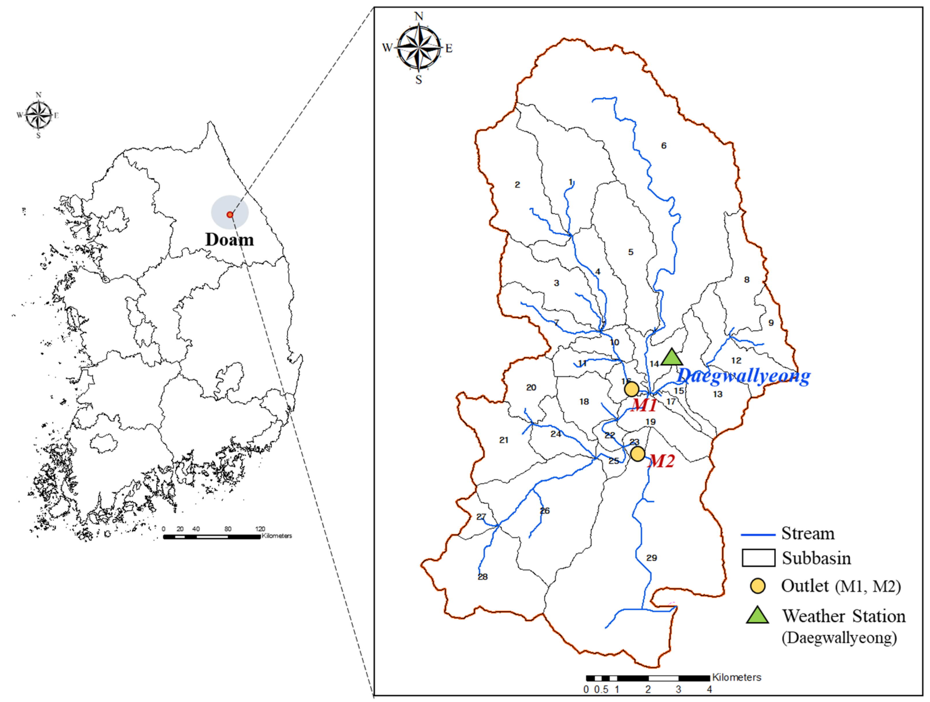
The Doam watershed, designated by the Ministry of Environment as a nonpoint source pollution management area (Figure 2), experiences recurring summer issues, including turbid water and water quality deterioration [36]. The slopes in the region vary widely, ranging from 14% to 53%, with an average slope of 30%, indicating the watershed’s steep topography. Moreover, the Doam watershed covers an area of 149 km2, with an average elevation of 913 m. Land use distribution in the Doam watershed is predominantly forest, covering 78.0% (116.0 km2) of the area. The agricultural area, including cultivated land, accounts for 8.4% (12.5 km2), urban areas make up 3.2% (4.7 km2), and other land uses comprise 10.5% (15.5 km2). Despite the relatively small proportion of agricultural land, agricultural activities occur on steep mountainous slopes, contributing significantly to sediment runoff and nonpoint source pollution. Due to this, along with the high SS concentrations, the watershed has been prioritized for continued national management efforts targeting nonpoint source pollution control. In this study, the Doam watershed was selected as the research site due to its designation and the need for a quantitative assessment of nonpoint source pollutant impacts on SS load, especially considering the interplay between land use, topography, and streamflow dynamics.

2.2. Model Description of SWAT and MUSLE

The SWAT model, developed by the Agricultural Research Service of the United States Department of Agriculture, is designed to simulate water quality over extended periods in large and complex watersheds. It enables spatiotemporal simulations of streamflow, baseflow, and soil erosion, making it particularly useful for assessing the effectiveness of various BMPs at the watershed scale. The SWAT model evaluates water resource management by analyzing streamflow and water quality under different management scenarios [37,38,39,40]. Moreover, soil erosion is estimated using the Modified Universal Soil Loss Equation (MUSLE), which improves upon the USLE by replacing rainfall energy with runoff energy to better simulate sediment transport under storm events [41,42,43,44,45,46]. The SWAT model operates as a process-based tool that delineates HRUs based on unique combinations of land use, slope, and soil type [24,47]. Despite its wide application, concerns have been raised regarding the model’s ability to accurately represent runoff and soil erosion in steep, agricultural terrains [33,35,48]. These limitations stem from the fact that SWAT’s core modules were developed using data collected in the gently sloped regions of the United States. The model may introduce streamflow and soil erosion prediction uncertainties when applied to steeper landscapes, such as the Doam watershed in South Korea. Jang et al. [33] indicated that the relationship between slope angle and slope length calculated by the default SWAT resulted in a spatial pattern that differed significantly from observed topographic characteristics in their study area, located in Haean-myeon, Yanggu-gun, South Korea. To address these limitations, this study integrated field-measured slope angles and slope lengths into each HRU to improve the estimation of topographic characteristics. In addition, regionally calibrated MUSLE parameters were applied, which enhanced the accuracy of streamflow and sediment simulations and improved the model’s reliability in evaluating BMP effectiveness in steep agricultural environments.

2.3. Application of SD-HRU and Modified MUSLE for Soil Erosion Management in SWAT

As previously mentioned, the distributions of slope lengths obtained from observations and those generated by SWAT differ considerably for HRU slope angles. When applied to steep watersheds, SWAT tends to underestimate slope length, which leads to errors in streamflow simulations that subsequently propagate to SS load estimations. To address this issue, this study applied observed slope angles and lengths from agricultural fields in the Doam watershed to individual HRUs. This approach was intended to minimize errors in streamflow and sediment simulations caused by topographic distortion. Accordingly, the slope angle and length calculated from actual measurements for each agricultural field and existing installed NPRFs were applied to the HRU, reflecting the actual agricultural field boundary.
Although SWAT calculates soil erosion for each HRU using the MUSLE equation, the coefficients and exponents of the MUSLE runoff factor were derived from rainfall–runoff data collected in the gently sloping Great Plains region of the United States. This limits its accuracy in simulating soil erosion in steeply sloped forested watersheds, such as those in South Korea [49,50]. The original MUSLE equation used a runoff factor coefficient of 11.8 and an exponent of 0.56. Unlike the USLE, which relies on rainfall energy to estimate erosion, the MUSLE replaces it with runoff energy by using total runoff volume ( Q surf ) and peak runoff rate ( q p e a k ) multiplied by HRU area ( A h r u ) as runoff energy factors. This change allows MUSLE to be more event-responsive; however, its parameters still require regional adaptation when applied to mountainous terrains.
In response, several studies have been conducted to estimate appropriate coefficients and exponents of the MUSLE runoff factor tailored to Korean watershed characteristics [51]. Lee et al. [34] modified SWAT to enable the application of land use-specific MUSLE parameters that reflect domestic conditions in South Korea (Equation (1)). This study applied the modified MUSLE to simulate soil erosion in the Doam watershed, providing a regionally accurate estimation of sediment yield in forested and agricultural areas. Based on the study by Lee et al. [34], the MUSLE coefficients (α) and exponents (β) were modified for each land use type to improve the accuracy of soil loss estimation in steeply sloped agricultural areas. To implement this approach, the SWAT source code was revised to allow land use-specific α and β values to be applied at the HRU. The values of α and β were determined so that the estimated soil loss per unit area for each land use type deviated by no more than 5% from reference values derived from national monitoring data and governmental reports. Specifically, the target values for rice paddies and forests were set to 0.168 ton/ha/yr and 0.055 ton/ha/yr, respectively, based on the updated base unit data provided by the National Institute of Environmental Research. For highland agricultural fields, the target soil loss was set to 55 tons/ha/yr, as recommended in the Ministry of Environment’s report on nonpoint source pollution reduction in upland areas. The coefficients and exponents were adjusted using pollutant loadings derived from the Korean Ministry of Environment’s unit load database, ensuring consistency with domestic hydrologic and land use characteristics.
S e d = α × ( A h r u × Q s u r f × q p e a k ) β × P U S L E × C U S L E × L S U S L E × K U S L E
where Sed is the soil erosion, Ahru is the area of HRU (ha), Qsurf is the surface runoff volume (mm/ha), Qpeak is the peak runoff (m3/sec), PUSLE is the support practice factor, CUSLE is the cover and management factor, LSUSLE is the topographic factor, and KUSLE is the soil erodibility factor.

2.4. SWAT Input Data Collection

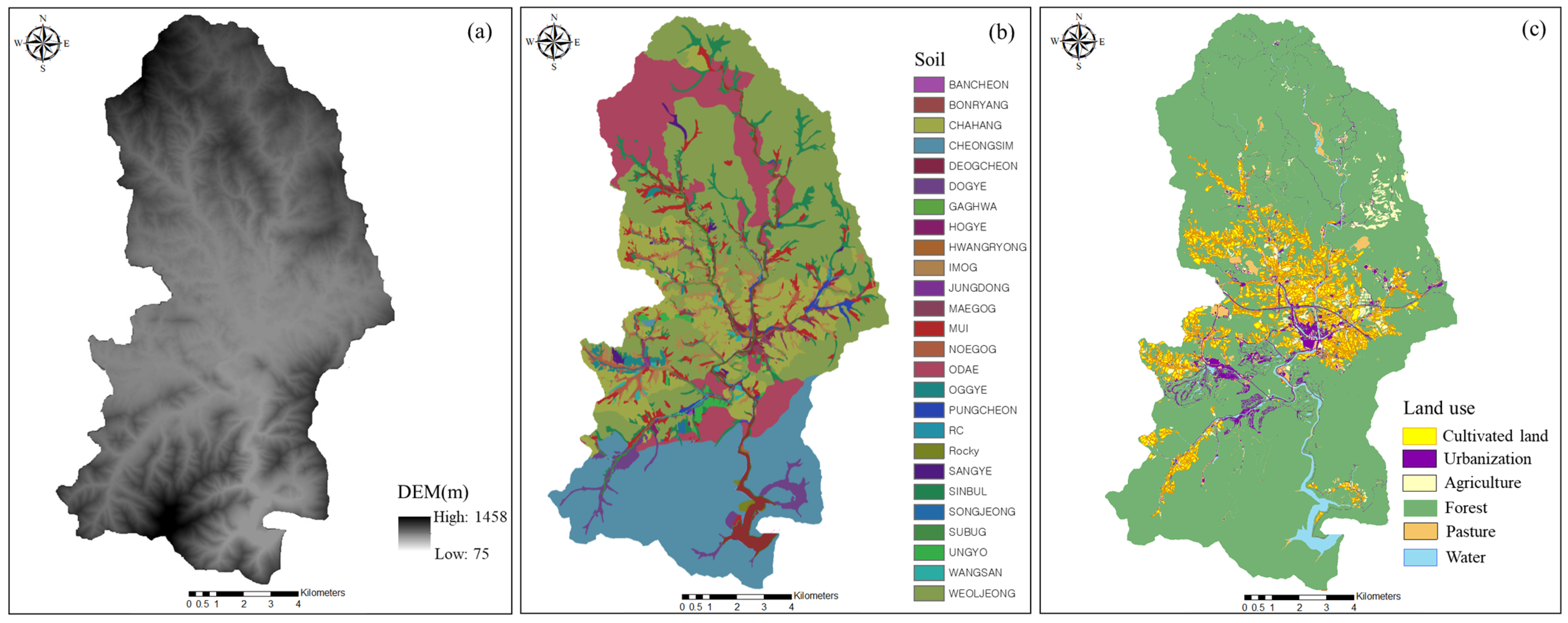
For this study, the necessary data for the SWAT modeling of the Doam watershed were collected, including topographic, land use, soil, and meteorological data. The National Geographic Information Institute (https://www.ngii.go.kr/eng/main.do) (accessed on 16 April 2025) provided a 30 m Digital Elevation Model (DEM). Land use data, with a spatial resolution of 30 m, was obtained from the Korea Ministry of Environment (https://egis.me.go.kr/req/intro.do) (accessed on 16 April 2025). Soil data were sourced from the Rural Development Administration’s detailed soil map (https://www.rda.go.kr) (accessed on 16 April 2025), which classifies soils into named mapping units based on local series characteristics. These soil units (e.g., BANCHEON, IMOG) were directly applied in the SWAT model classification to maintain region-specific hydrologic behavior (Figure 3). Moreover, meteorological data used for SWAT model inputs were obtained from three Korea Meteorological Administration (KMA) weather stations (https://data.kma.go.kr/) (accessed on 16 April 2025), including one station (Daegwallyeong) located in the Doam watershed and two stations located outside the watershed boundary and not in its immediate vicinity, which were additionally considered to account for the spatial variability of meteorological inputs. The dataset includes daily records from 2010 to 2019, covering maximum and minimum temperatures, precipitation, average wind speed, and relative humidity. Table 1 presents the annual and seasonal precipitation over the past 10 years based on data from the weather station located in the Doam watershed. The 10-year average annual precipitation (2010–2019) recorded at this station was 1275 mm, with the year 2012 recording 1289 mm, which is the closest to the 10-year average.

2.5. Evaluation of SWAT Performance Through Calibration and Validation

The SWAT-CUP, which stands for Calibration and Uncertainty Programs, was developed at the Swiss Federal Institute of Aquatic Science and Technology in Switzerland to facilitate the calibration and validation process in hydrologic modeling using SWAT [52]. The SWAT-CUP is an independent program that provides several model calibration and validation algorithms, such as Sequential Uncertainty Fitting ver.2 (SUFI2), Generalized Likelihood Uncertainty Estimation (GLUE), Parameter Solutions (ParaSol), Markov Chain Monte Carlo (MCMC), and Particle Swarm Optimization (PSO) [52]. The optimization algorithm for calibration and validation is SUFI2, which is the easiest to use among the five algorithms provided by the SWAT-CUP and has been validated for its usefulness in various previous studies [53,54,55,56,57,58,59].
Observed daily streamflow and SS data collected from the Doam watershed during 2012–2019 for nonpoint source pollution management were used to calibrate and validate the SWAT model. The SWAT model was used to simulate daily streamflow and SS load from 2008 to 2019, with model calibration and validation conducted using the SUFI2 algorithm of SWAT-CUP. All statistical analyses were also performed using SWAT-CUP. A warming-up period was established from 2008 to 2012 to stabilize the model parameters, followed by calibration (2012–2014) and validation (2015–2019) periods. In this study, soil erosion for forest and highland cropland was estimated using the coefficients and exponents of the MUSLE runoff factor. Therefore, the calibration and validation of the SS load were conducted using only the parameters affecting the SS load, excluding parameters like USLE_K and USLE_P, which could directly influence soil erosion results. To evaluate the model’s performance, streamflow and SS data were collected from two monitoring stations (M1: upstream, M2: downstream) located in the upstream and downstream parts of the watershed, respectively. These stations were selected based on their hydrological representativeness and suitability for field monitoring. M1, located in the upper part of the watershed, consistently exhibited high SS concentrations throughout the observation period, making it suitable for analyzing sediment dynamics in steep and erosion-prone areas. M2, situated at the downstream outlet where tributaries converge with the main stream, was chosen to capture the integrated hydrological response of the entire watershed, allowing for a comprehensive assessment of streamflow and sediment export. The calibration period was set from 2012 to 2014, and validation was conducted using data from 2015 to 2019. At both stations, streamflow and SS measurements were obtained across a range of hydrological conditions to capture temporal variability. For streamflow, 46 observations were used for calibration, and 36 and 42 observations were used for validation at M1 and M2, respectively. For SS, 46 calibration samples were collected at both sites, with 30 and 36 validation samples at M1 and M2, respectively. The number of observations differed slightly between the stations due to variations in field accessibility and weather conditions during the monitoring. These observational datasets formed the basis for model calibration and validation, enabling reliable simulation of hydrological and sediment transport processes within the watershed.
The performance of the SWAT model was evaluated using various statistical indices, including the coefficient of determination (R2), Nash–Sutcliffe Model Efficiency (NSE), index of agreement (IOA), and Kling–Gupta Efficiency (KGE) [60,61]. These indices are widely used as model evaluation metrics to assess model performance. Most of them range from 0 to 1, with 1 indicating a perfect match between observed and simulated values. However, the NSE can range from −∞ to 1, where values closer to 1 indicate better model performance, and values below 0 indicate that the model predictions are worse than the mean of the observed data. R2 measures the strength of the linear relationship between measured data and simulated results, indicating how well the model explains variance in the observed data. NSE, commonly used in hydrologic modeling, compares the variance of residuals with the variance of observed data, making it useful for evaluating prediction accuracy. Unlike NSE, which can yield negative values indicating poor model performance, IOA always remains between 0 and 1. By accounting for both the magnitude and trend of variations, IOA provides a more comprehensive measure of model agreement. In addition, the KGE was employed to provide a more integrated evaluation by simultaneously considering correlation, bias, and variability between observed and simulated values. This metric helps compensate for the limitations of individual indices like NSE and R2 when used alone. The formulas for these indices are presented in Equations (2)–(5).
R 2 = ( i = 1 n ( O o b s , i O ¯ o b s ) S s i m , i S ¯ s i m i = 1 n ( O o b s , i O ¯ o b s ) 2 i = 1 n ( S s i m , i S ¯ s i m ) 2 ) 2
N S E = 1 i = 1 n ( O o b s , i S s i m , i ) 2 i = 1 n ( O o b s , i O ¯ o b s ) 2
I O A = 1 i = 1 n ( O o b s , i S s i m , i ) 2 i = 1 n ( S s i m , i O ¯ o b s + O o b s , i O ¯ o b s ) 2
K G E = 1 ( r 1 ) 2 + ( β 1 ) 2 + ( γ 1 ) 2
where O o b s , i is the observation, S s i m , i is the simulation, O ¯ o b s is the mean of the observations, S ¯ s i m is the mean of the simulations, and n is the total number of observations.
In addition, in the equation for KGE, r is the Pearson correlation coefficient between the observed and simulated values, β = S ¯ s i m O ¯ o b s is the bias ratio, and γ = σ s i m / S ¯ s i m σ o b s / O ¯ o b s is the variability ratio, where σ o b s and σ s i m are the standard deviations of the observed and simulated values, respectively.

2.6. Integrated BMP Strategies for Soil Erosion Control and SS Load Reduction

This study applied the SWAT model to estimate soil erosion rates (tons/ha/year) in each subbasin and identify priority areas for intervention based on key watershed characteristics, including high-altitude farmland, elevation, and slope gradient, which significantly influence erosion and deposition patterns. Subbasins with the highest soil erosion were prioritized for targeted management.
To mitigate soil erosion, BMP strategies were designed to align with the specific environmental conditions of the study area (Table 2). Two management scenarios were evaluated: Scenario 1, representing ongoing BMP projects in the Doam watershed, and Scenario 2, which incorporated additional BMPs to further reduce erosion through supplementary measures. This comparative approach assessed the effectiveness of existing and enhanced BMP interventions in controlling soil erosion and SS load at the watershed scale.
The implemented BMPs included riparian vegetative buffer zones, which converted farmland near streams into vegetation-dominated areas to filter sediment and pollutants. Slope reduction in this study refers to the construction of terraces in steep croplands, a common practice in high-altitude farmland. While this approach effectively reduces slope length and surface runoff, it also creates risers that may be prone to localized erosion. Additional measures included slope protection structures (e.g., terraces, retention walls) to control soil displacement, water channel systems to enhance drainage and regulate flow velocity, and soil surface cover practices (e.g., straw mulching) to protect exposed soils from rainfall-induced erosion. Onion mesh bags were distributed to stabilize bare soils, particularly during the rainy season. Unauthorized cultivated lands were restored to their natural state, while rehabilitated dug channels improved water flow and SS transport efficiency.
Scenario 1 focused on the selective implementation of BMPs, targeting critical erosion-prone areas with slope protection structures, water channel systems, soil surface cover, onion mesh bag distribution, dug channel restoration, and restoration of unauthorized cultivated lands. In contrast, Scenario 2 adopted a more comprehensive BMP strategy, integrating all BMPs into a single, holistic management plan. This scenario expanded upon Scenario 1 by incorporating fallowing marginal farmland, slope reduction in high-altitude fields, and the establishment of vegetative buffer zones in both agricultural and riparian areas. These additional measures enhanced soil stabilization and erosion control by reducing surface runoff velocity, improving infiltration capacity, and intercepting sediment transport before it reached water bodies. By implementing a broader range of BMPs at a larger spatial scale, Scenario 2 aimed to maximize soil erosion reduction efficiency by addressing multiple erosion sources and stabilizing vulnerable landscapes. In both scenarios, BMPs were applied exclusively to cropland areas, which were identified as the main contributors to soil erosion within the watershed. Reduction efficiencies for each BMP were quantified by comparing simulation results from each scenario to a baseline condition without any BMP implementation, focusing on soil loss reduction per unit area at the subbasin.
To assess the relative effectiveness of individual BMPs in controlling soil erosion, this study analyzed the soil erosion reduction efficiency of each BMP across subbasins. Furthermore, subbasin soil erosion reduction efficiency was evaluated under each scenario, enabling the prioritization of high-risk management areas.

3. Results and Discussion

3.1. Calibration and Validation Results of MUSLE and SWAT for SS Load Simulation

Table 3 presents the coefficients and exponents of the MUSLE runoff factor estimated for forests and steep-slope cultivated lands in the Doam watershed. The runoff factor exponents for forests and highland cultivated lands were found to be similar to the value of 0.55 proposed by Williams [41]. However, the coefficients were estimated at 2.80 and 0.33, which are 76% and 97% lower than the values suggested by Williams [41], respectively.
Similarly, in a study by Lee et al. [34], the coefficients and exponents of the runoff factor for forests in the Gaa watershed, designated as a nonpoint pollution management area, were estimated at 0.14 and 0.60, respectively. These findings highlight that the coefficients and exponents of the MUSLE runoff factor can vary significantly depending on the watershed’s climatic and topographical characteristics. The results suggest that the unique conditions of the Doam watershed strongly influence the runoff factor, underscoring the need for region-specific adjustments.
Therefore, appropriately calibrating the MUSLE runoff factor coefficients and exponents is essential for accurate simulation in South Korean watersheds. This approach will enhance soil conservation planning and improve the effectiveness of BMP applications for soil erosion reduction.
The optimized parameters derived using SWAT-CUP are presented in Table 4. Sensitivity analysis identified key parameters for streamflow and SS load calibration. For streamflow, the most sensitive parameters were the SCS runoff curve number (CN2) and the baseflow alpha factor (ALPHA_BF), which play a critical role in simulating surface runoff and baseflow processes that shape the watershed’s hydrological response.
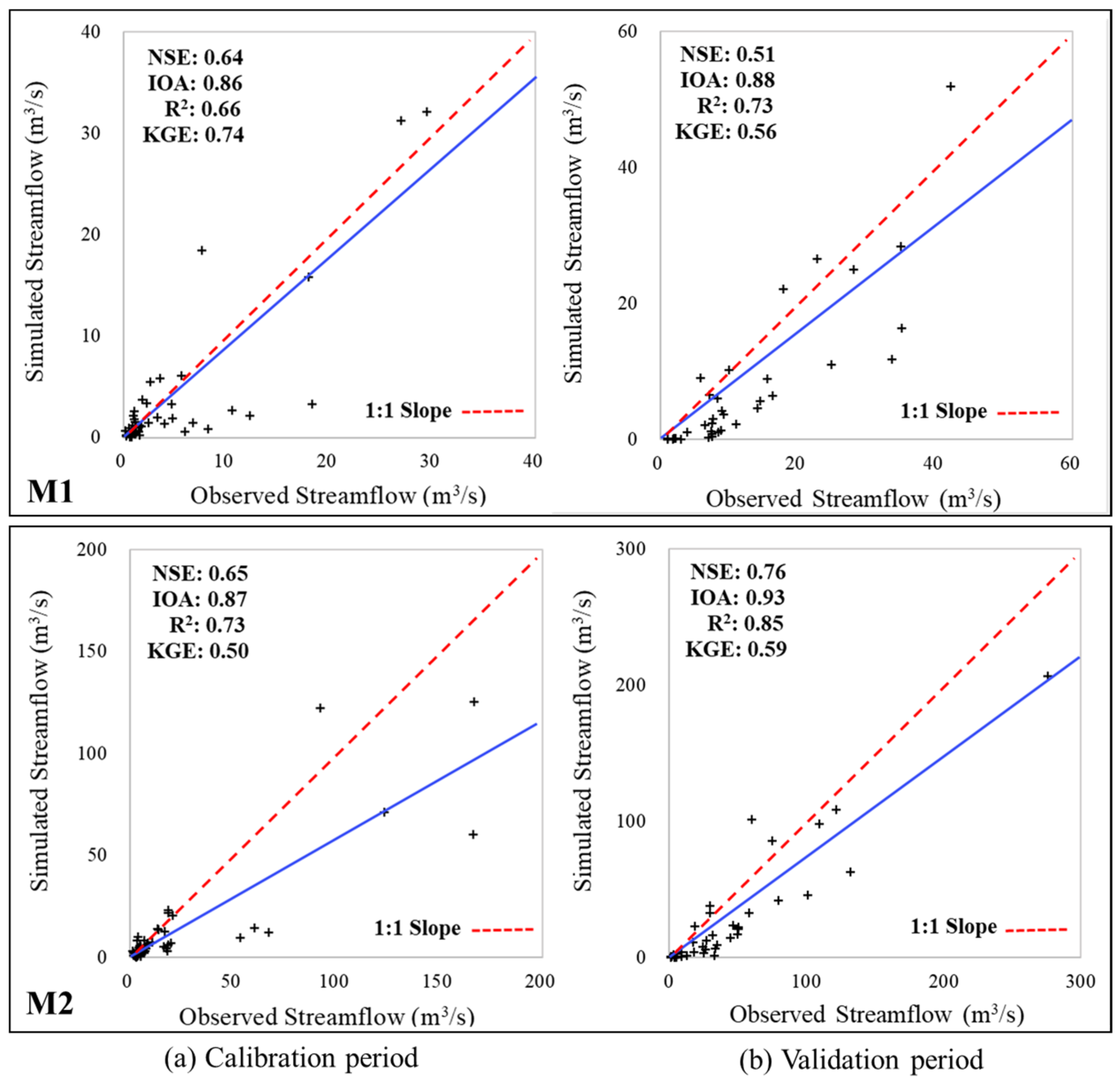
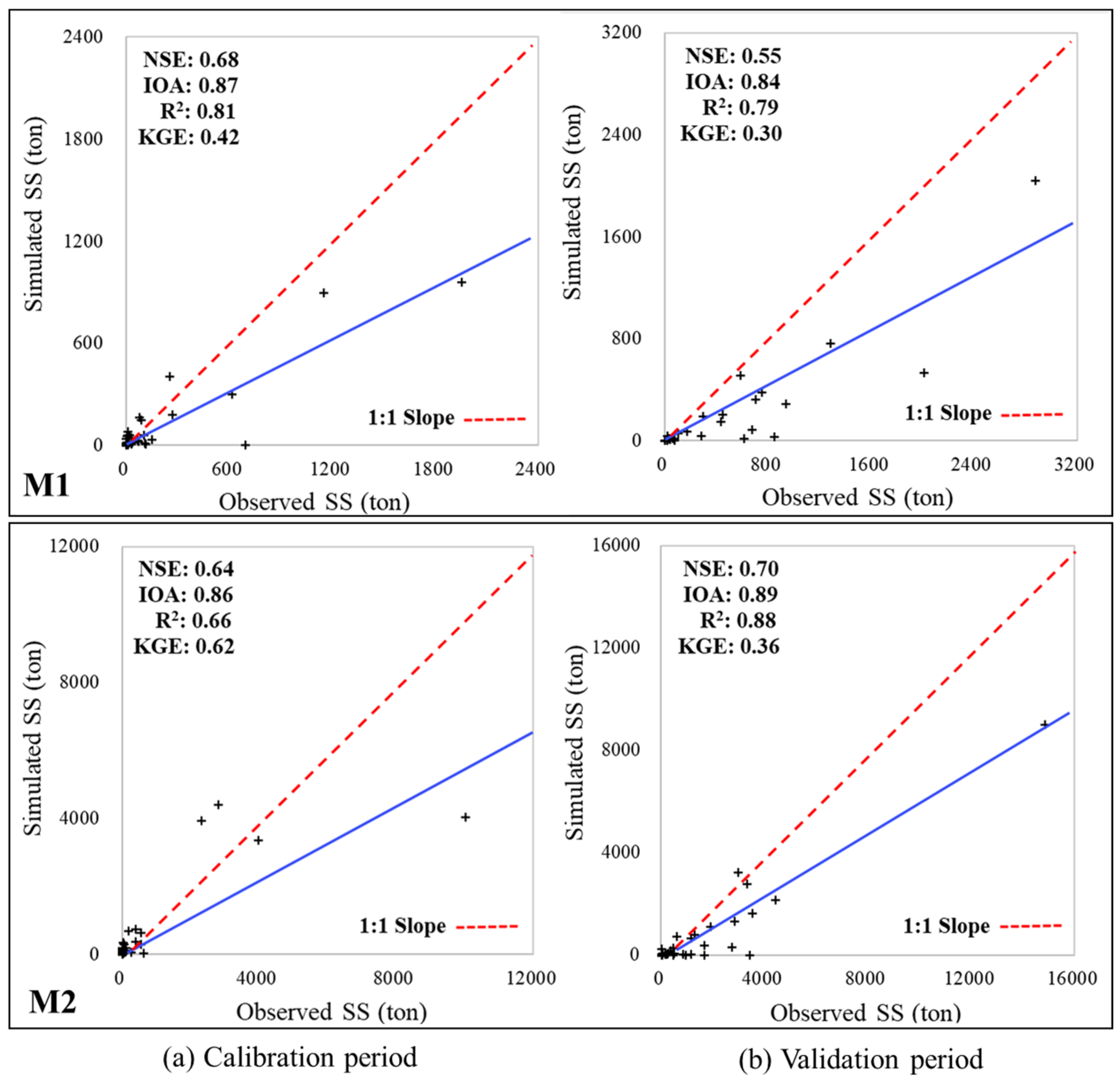
For SS load calibration, the sediment entrainment exponent (SPEXP) and the peak rate adjustment factor for sediment routing (ADJ_PKR) were highly sensitive. These parameters significantly influence sediment transport dynamics and channel processes, emphasizing their importance in accurately simulating SS load. The calibration and validation of the SWAT model for streamflow during 2012–2019 demonstrated robust performance, as shown in Figure 4. During the calibration period, the model achieved NSE values of 0.64–0.65, R2 values of 0.66–0.73, and IOA values of 0.86–0.87, indicating satisfactory to very good performance. Validation results showed slightly wider ranges, with NSE values of 0.51–0.76, R2 values of 0.73–0.85, and IOA values of 0.88–0.93, confirming the model’s reliability under varying hydrological conditions. For the SS simulation (Figure 5), the calibration period yielded NSE values of 0.64–0.68, R2 values of 0.66–0.81, and IOA values of 0.86–0.87, reflecting very good model performance. The validation period produced NSE values of 0.55–0.70, R2 values of 0.79–0.88, and IOA values of 0.84–0.89, indicating good agreement between observed and simulated SS loads. While some peak values, especially in upstream locations, were underpredicted, this tendency is a limitation in hydrologic models due to difficulties in accurately predicting extreme streamflow events and the resulting high sediment concentrations. However, the overall period trends and statistical indicators (NSE, R2, IOA) suggest that the model still provides reliable estimates. This is further supported by higher KGE values at the downstream site (M2), which reflect better agreement under integrated watershed responses. Although the KGE values at the upstream site (M1) were relatively low during both the calibration (0.42) and validation (0.30) periods, which reflects limitations in simulating SS load under certain hydrological conditions, the downstream site (M2) showed considerably better performance, achieving KGE values of 0.62 and 0.36, respectively. Moreover, this underperformance at M1 is partially attributed to greater variability in streamflow and SS load at the headwater site, where localized peaks are more difficult to capture accurately. Nevertheless, other statistical indicators (NSE, R2, IOA) demonstrated strong agreement at both monitoring locations, especially M2, where simulated and observed values showed consistent trends. According to Moriasi et al. [61], these combined performance statistics classify the model as “Satisfactory” across two monitoring stations. Despite slight reductions in NSE and KGE values during the validation phase, the overall model reliability remained satisfactory. The SWAT model, calibrated and validated using SWAT-CUP, exhibited reasonable capability in simulating both streamflow and SS load dynamics in the Doam watershed, making it suitable for scenario-based evaluations of BMPs for soil erosion reduction in watershed management.

3.2. Effectiveness of BMPs in Soil Erosion Reduction

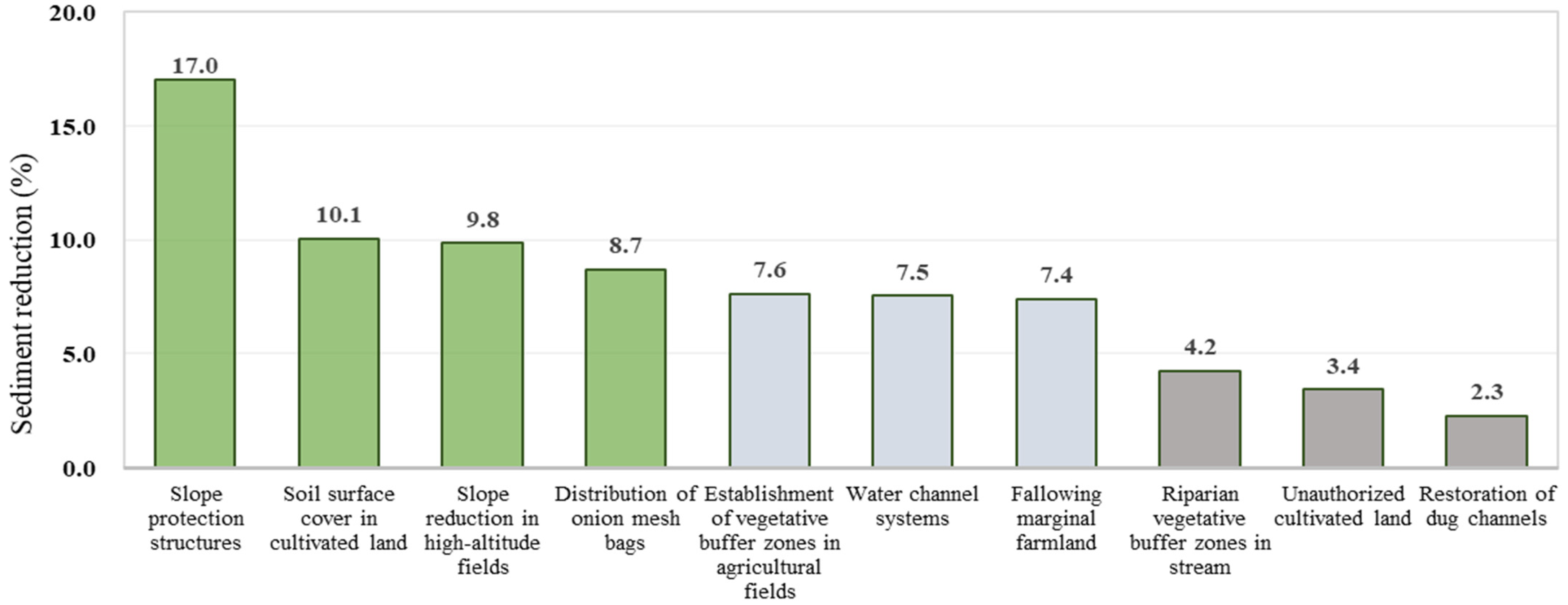
Figure 6 presents the ranking of BMPs based on their relative effectiveness in soil erosion reduction. Among the analyzed BMPs, slope protection structures exhibited the highest effectiveness, achieving a 17.0% reduction in soil erosion, the greatest among all measures. This high efficiency is attributed to their ability to stabilize steep slopes and minimize soil displacement by mitigating surface runoff. Unlike other BMPs that primarily focus on filtering or slowing sediment transport, slope protection structures address soil erosion at its source by reinforcing vulnerable slopes. Furthermore, these reduction efficiencies were calculated by comparing each individual BMP scenario with the baseline condition (without BMP), focusing on soil erosion reduction per unit area at the subbasin scale. The values represent the relative effectiveness of each BMP in reducing soil loss per unit area from agricultural land. Within the SWAT model, these structures were implemented through the Operations file using terrain modification and stabilization parameters, ensuring a substantial reduction in soil erosion.
Soil surface cover in cultivated land ranked second, demonstrating a 10.1% reduction in soil erosion, followed by slope reduction in high-altitude fields (9.8%), onion mesh bag distribution (8.7%), and vegetative buffer zones in agricultural fields (7.6%). In contrast, unauthorized cultivated land restoration (3.4%) and dug channel restoration (2.3%) exhibited the lowest effectiveness, indicating their limited contribution to reducing soil erosion within agricultural subbasins. Although BMPs were applied only to cropland areas, which represent a relatively small portion of the watershed, their implementation significantly reduced overall soil erosion due to the high erosion potential of agricultural lands. However, it is essential to clarify that this study focused on evaluating the relative effectiveness of individual BMPs in reducing soil erosion at the subbasin scale, based on upland sediment generation. Therefore, in-stream interventions such as riverbank stabilization or in-channel sediment retention measures were not examined. Although riparian buffer zones were included among the BMPs, their role was limited to reducing sediment inflow from adjacent land areas rather than directly altering sediment transport processes within the stream channel. Nevertheless, in certain cases, reductions in sediment input can alter channel dynamics, potentially leading to increased channel erosion due to sediment transport imbalances. Although this aspect was beyond the scope of this study, it may be considered for further investigation in future research. The primary objective of this study was to reduce soil loss predominantly generated from steep agricultural areas by applying BMPs specifically to cropland. Accordingly, BMPs were applied only to agricultural land use—specifically croplands—where actual land use, topography, and field-scale applicability justified their implementation. Moreover, BMPs were not simulated for forested or urban land uses due to their naturally low erosion rates and practical management constraints. Although various land use types exist within the watershed, BMPs in both scenarios were applied exclusively to agricultural areas where practical feasibility and applicability were deemed high.

3.3. Scenario-Based Assessment of SS Load and Soil Erosion Reduction

A comparative summary of the annual soil erosion and SS concentrations, along with their respective reduction efficiencies for each scenario, is presented in Table 5. The results clearly demonstrate that Scenario 2 achieved the highest reduction efficiency, underscoring the benefits of an integrated BMP approach. Under baseline conditions, the total soil erosion in the watershed was estimated at 2913 tons/ha/year. Implementation of Scenario 1 reduced soil erosion to 1904 tons/ha/year, achieving a 34.6% reduction. The broader BMP application in Scenario 2 further reduced soil erosion to 1185 tons per year, corresponding to a 59.3% reduction compared to baseline conditions. These results indicate that the comprehensive BMP strategy in Scenario 2 was substantially more effective in minimizing soil erosion than the more selective approach in Scenario 1.
In addition to soil erosion reduction, the impact of BMPs on in-stream SS concentrations was analyzed. The baseline SS concentration in the river system was estimated at 32.3 mg/L. Under Scenario 1, BMP implementation led to a reduction in SS concentration to 21.0 mg/L, corresponding to a 35.0% improvement. The enhanced BMP application in Scenario 2 further reduced SS concentration to 13.8 mg/L, achieving a 57.3% improvement over baseline conditions. These findings demonstrate that BMP implementation not only reduced soil erosion at the watershed scale but also significantly improved in-stream sediment conditions. This improvement in water quality was primarily driven by a decrease in sediment input and associated reductions in suspended sediment concentration rather than changes in discharge. As a result, aquatic ecosystem health was enhanced through lower sediment loads in streamflow. The greater effectiveness of Scenario 2 in reducing in-stream SS concentrations can be attributed to its expanded BMP application, particularly the integration of riparian buffer zones and additional soil erosion control measures. These practices played a crucial role in intercepting sediment before it entered the stream network, thereby mitigating sediment transport and improving downstream water quality. The substantial improvement in SS concentrations under Scenario 2 underscores the importance of comprehensive BMP strategies in achieving effective soil erosion and sediment control at the watershed scale.

3.4. Soil Erosion Reduction and Subbasin Prioritization for Sustainable Watershed Management

This study evaluated soil erosion reduction efficiency across 29 subbasins (Figure 2) under two BMP implementation scenarios, revealing significant spatial variations in erosion control effectiveness (Table 6). Scenario 1, representing the BMPs currently implemented in the Doam watershed, resulted in reduction efficiencies ranging from 0.4% (Subbasin 29) to 64.7% (Subbasin 27). These values represent the relative reduction in soil erosion simulated within each subbasin, calculated by comparing erosion amounts under baseline and BMP scenarios. Each subbasin’s efficiency reflects internal erosion changes due to BMP implementation.
The highest efficiencies were observed in Subbasins 27 (64.7%), 5 (55.9%), and 21 (51.7%), while the lowest reductions were recorded in Subbasins 25 (1.3%), 17 (1.2%), and 29 (0.4%). The notable soil erosion stabilization in Subbasins 27, 5, and 21 was primarily attributed to the implementation of slope protection structures, soil surface cover in cultivated land, and onion mesh bag distribution, which effectively reduced surface runoff velocity, enhanced soil infiltration capacity, and intercepted soil erosion transport along slopes.
Scenario 2, which incorporated an expanded BMP strategy applied on a broader scale, significantly improved soil erosion reduction efficiency across all subbasins, with reductions ranging from 1.3% (Subbasin 25) to 70.5% (Subbasin 27). The highest reductions were observed in Subbasins 27 (70.5%), 5 (69.1%), and 26 (68.2%), while the lowest efficiency improvements, despite enhanced BMP applications, were recorded in Subbasins 29 (8.1%), 23 (1.4%), and 25 (1.3%). Scenario 2 consistently outperformed Scenario 1 across all subbasins, with the most pronounced efficiency gains observed in Subbasins 10, 14, and 26, where the enhanced BMP strategies achieved significantly greater reductions in soil erosion.
Unlike Scenario 1, which implemented a limited set of BMPs, Scenario 2 incorporated vegetative buffer zones, dug channel restoration, and unauthorized cultivated land management, enabling more effective targeting of high-erosion risk areas. The variations in soil erosion reduction efficiency among subbasins were largely influenced by land use and hydrological characteristics. Subbasins with extensive agricultural land, such as Subbasins 5, 11, and 27, exhibited higher reduction efficiencies due to the strong influence of BMPs, particularly slope reduction in high-altitude fields, establishment of vegetative buffer zones in agricultural fields, and restoration of dug channels, which effectively reduced surface runoff velocity, improved soil infiltration, and intercepted soil erosion transport along slopes.
In contrast, Subbasins 23, 25, and 29, which are predominantly forested or water-dominated areas with minimal agricultural land, exhibited relatively lower efficiency improvements. The naturally low soil erosion rates in these subbasins, due to dense vegetation cover, high organic matter content, and stable soil conditions, reduced the overall impact of BMP implementation. Consequently, BMPs had a more pronounced effect in agricultural subbasins, where erosion control measures directly influenced hydrological processes. In contrast, their effectiveness was limited in forested and water-dominated areas, not only due to naturally low erosion rates but also because BMPs were not simulated for these land-use types in this study. These findings underscore the importance of subbasin-specific BMP applications, particularly in high-risk agricultural areas. While it may appear intuitive that BMPs would have more impact where agricultural land is concentrated, the model provided valuable spatial quantification of erosion risk and BMP effectiveness, enabling prioritization of subbasins based not only on land use proportion but also on terrain, slope, and erosion response. These findings are consistent with previous studies that demonstrated higher BMP effectiveness in steep agricultural regions due to concentrated runoff and erosion-prone conditions [35]. Unlike studies that applied uniform BMP strategies, this study highlights the benefits of tailoring BMP applications based on spatial characteristics within a watershed [62].
The spatial variability in soil erosion reduction efficiency suggests that a targeted BMP implementation strategy, tailored to subbasin-specific characteristics, can maximize soil erosion reduction and improve watershed sustainability. This variability has important management implications, as it indicates that allocating BMPs uniformly across a watershed may not be cost-effective. Subbasins with high erosion potential and responsive land use conditions should be prioritized for intervention to achieve maximum sediment control with limited resources.
It should be noted that since BMPs were applied exclusively to cropland subbasins in this study, the reduction efficiencies are inherently influenced by the distribution and extent of agricultural land across subbasins. Future research will supplement this approach by incorporating forest and channel dynamics to evaluate integrated sediment control under diverse watershed conditions more comprehensively. While the findings provide valuable insights for erosion control in steep, agriculture-dominated watersheds under temperate monsoon conditions, their direct applicability to regions with markedly different topographic or climatic conditions may be limited. However, the proposed approach can be reasonably extended to watersheds with similar erosion-prone characteristics, particularly those sharing comparable land use, slope, and rainfall patterns.

4. Conclusions

This study aimed to evaluate long-term streamflow and SS load using SWAT, which incorporates spatially distributed farmland characteristics and adjusted MUSLE parameters, and to propose soil erosion reduction measures by applying individual BMPs and comprehensive management scenarios. Additionally, priority management areas for cropland were identified based on the soil erosion reduction efficiency between subbasins, providing a framework for optimizing BMP selection and placement.
The results highlight the importance of spatially adaptive BMP implementation, demonstrating substantial soil erosion and SS concentration reduction efficiencies across different management scenarios. The effectiveness of BMPs varied depending on subbasin characteristics, such as land use, topography, and hydrological conditions. Agricultural areas with steep slopes and intensive cultivation exhibited greater reductions in soil erosion. Scenario-based BMP applications further revealed spatial differences in soil erosion reduction efficiency, emphasizing the need for site-specific management approaches to achieve optimal results.
A targeted BMP implementation strategy, tailored to subbasin-specific conditions, is essential for maximizing soil erosion reduction and improving watershed sustainability. Identifying priority management areas based on soil erosion reduction efficiency can enhance the effectiveness of erosion control efforts, ensuring that high-risk areas receive appropriate interventions. These findings provide practical insights for policymakers and watershed managers in developing cost-effective and scientifically grounded erosion control strategies. Based on these findings, future research should further refine integrated modeling approaches that combine spatial prioritization and scenario-based BMP evaluation. In particular, optimizing BMP selection and placement strategies across varying watershed conditions, including nonagricultural areas, will be essential to improve model applicability and guide more comprehensive watershed management. These findings can support policymakers in developing spatially targeted erosion control programs by identifying high-priority subbasins where BMP investment would yield the greatest benefit. Future research should also explore the integration of these modeling results with cost-effectiveness analysis to inform funding allocation and policy prioritization at the watershed. The findings of this study can be applied to identify high-risk subbasins, guide BMP selection, and support the development of efficient soil erosion management strategies in vulnerable watersheds. These insights contribute to the establishment of evidence-based soil conservation plans, promoting more effective and sustainable erosion control practices across various watershed environments.

Author Contributions

Conceptualization, J.L.; methodology, J.L.; formal analysis, J.L. and M.S.; data curation, J.L. and S.L.; writing—original draft preparation, J.L.; writing—review and editing, J.L. and S.L.; visualization, J.L. and W.J.P.; supervision, K.J.L. All authors have read and agreed to the published version of the manuscript.

Funding

This research was supported by Environmental Fundamental Data Examination project of Hangang River Basin Management Committee.

Institutional Review Board Statement

Not applicable.

Data Availability Statement

The datasets that support the findings of this study are available from the first author upon reasonable request.

Conflicts of Interest

The authors declare no conflicts of interest.

References

  1. Jin, G.; Li, Z.; Deng, X.; Yang, J.; Chen, D.; Li, W. An analysis of spatiotemporal patterns in Chinese agricultural productivity between 2004 and 2014. Ecol. Indic. 2019, 105, 591–600. [Google Scholar] [CrossRef]
  2. Wang, Y.; Bian, J.; Zhao, Y.; Tang, J.; Jia, Z. Assessment of future climate change impacts on nonpoint source pollution in snowmelt period for a cold area using SWAT. Sci. Rep. 2018, 8, 2402. [Google Scholar] [CrossRef] [PubMed]
  3. Zeiger, S.J.; Owen, M.R.; Pavlowsky, R.T. Simulating nonpoint source pollutant loading in a karst basin: A SWAT modeling application. Sci. Total Environ. 2021, 785, 147295. [Google Scholar] [CrossRef]
  4. Wang, Y.; Wu, C.; Zhao, Z.; Yu, B.; Liu, G. Assessing spatiotemporal heterogeneity of coastal organic nonpoint source pollution via soil erosion in Yellow River Delta, China. Ecol. Indic. 2024, 166, 112519. [Google Scholar] [CrossRef]
  5. Harano, F.K.F.; Galvanin, E.A.S. Spatio-temporal assessment of potential nonpoint pollution risk sources in the Chavantes reservoir basin, Brazil. J. S. Am. Earth Sci. 2025, 152, 105310. [Google Scholar] [CrossRef]
  6. Zheng, Y.; Han, F.; Tian, Y.; Wu, B.; Lin, Z. Chapter 5—Addressing the uncertainty in modeling watershed nonpoint source pollution. In Ecological Modeling and Engineering of Lakes and Wetlands; Elsevier: Amsterdam, The Netherlands, 2014; Volume 26, pp. 113–159. [Google Scholar]
  7. Zuo, D.; Bi, Y.; Song, Y.; Xu, Z.; Wang, G.; Ma, G.; Abbaspour, K.C.; Yang, H. The response of nonpoint source pollution to land use change and risk assessment based on model simulation and grey water footprint theory in an agricultural river basin of Yangtze river, China. Ecol. Indic. 2023, 154, 110581. [Google Scholar] [CrossRef]
  8. Zhang, T.; Yang, Y.; Ni, J.; Xie, D. Adoption behavior of cleaner production techniques to control agricultural nonpoint source pollution: A case study in the Three Gorges Reservoir Area. J. Clean. Prod. 2019, 223, 897–906. [Google Scholar] [CrossRef]
  9. Zou, L.L.; Liu, Y.S.; Wang, Y.S.; Hu, X.D. Assessment and analysis of agricultural nonpoint source pollution loads in China: 1978–2017. J. Environ. Manag. 2020, 263, 110400. [Google Scholar] [CrossRef]
  10. Hussain, F.; Ahmed, S.; Naqvi, S.M.Z.A.; Awais, M.; Zhang, Y.; Zhang, H.; Raghavan, V.; Zhang, Y.; Zhao, G.; Hu, J. Agricultural Non-Point Source Pollution: Comprehensive Analysis of Sources and Assessment Methods. Agriculture 2025, 15, 531. [Google Scholar] [CrossRef]
  11. Nuruzzaman, M.; Bahar, M.M.; Naidu, R. Diffuse soil pollution from agriculture: Impacts and remediation. Sci. Total Environ. 2025, 962, 178398. [Google Scholar] [CrossRef]
  12. Xue, B.; Zhang, H.; Wang, G.; Sun, W. Evaluating the risks of spatial and temporal changes in nonpont source pollution in a Chinese river basin. Sci. Total Environ. 2022, 807, 151726. [Google Scholar] [CrossRef] [PubMed]
  13. Badrzadeh, N.; Samani, J.M.V.; Mazaheri, M.; Kuriqi, A. Evaluation of management practices on agricultural nonpoint source pollution discharges into the rivers under climate change effects. Sci. Total Environ. 2022, 838, 156643. [Google Scholar] [CrossRef] [PubMed]
  14. Firoozi, A.A.; Firoozi, A.A. Water erosion processes: Mechanisms, impact, and management strategies. Results Eng. 2024, 24, 103237. [Google Scholar] [CrossRef]
  15. He, X.; Miao, Z.; Wang, Y.; Yang, L.; Zhang, Z. Response of soil erosion to climate change and vegetation restoration in the Ganjiang River Basin, China. Ecol. Indic. 2024, 158, 111429. [Google Scholar] [CrossRef]
  16. Issaka, S.; Ashraf, M.A. Impact of soil erosion and degradation on water quality: A review. Geol. Ecol. Landsc. 2017, 1, 1–11. [Google Scholar] [CrossRef]
  17. Eekhout, J.P.C.; Vente, J.D. Global impact of climate change on soil erosion and potential for adaptation through soil conservation. Earth-Sci. Rev. 2022, 226, 103921. [Google Scholar] [CrossRef]
  18. Xie, H.; Chen, L.; Shen, Z. Assessment of agricultural best management practices using models: Current issues and future perspectives. Water 2015, 7, 1088–1108. [Google Scholar] [CrossRef]
  19. Liu, Y.; Wang, R.; Guo, T.; Engel, B.A.; Flanagan, D.C.; Lee, J.G.; Li, S.; Pijanowski, B.C.; Collingsworth, P.D.; Wallace, C.W. Evaluating efficiencies and cost-effectiveness of best management practices in improving agricultural water quality using integrated SWAT and cost evaluation tool. J. Hydrol. 2019, 577, 123965. [Google Scholar] [CrossRef]
  20. Liu, Y.; Yang, W.; Bass, B.; Rao, Y.R. Effectiveness of agricultural BMPs on phosphorus load reduction for the Canadian Lake Erie Basin: A literature review. Environ. Rev. 2025, 33, 1–24. [Google Scholar] [CrossRef]
  21. Wang, D.; Gao, X.; Wu, S.; Zhao, M.; Zheng, X.; Wang, Z.; Zhang, Y.; Fan, C. A Comprehensive review on ecological buffer zone for pollutants removal. Water 2024, 16, 2172. [Google Scholar] [CrossRef]
  22. Xu, L.; Liu, X.; Chen, J.; Li, J.; Yu, Y.; Ma, X. Efficiency assessment of best management practices in sediment reduction by investigating cost-effective tradeoffs. Agric. Water Manag. 2022, 265, 107546. [Google Scholar]
  23. Fakouri, B.; Mazaheri, M.; Samani, J.M. Management scenarios methodology for salinity control in rivers (case study: Karoon River, Iran). J. Water Supply Res. Technol. AQUA 2019, 68, 74–86. [Google Scholar] [CrossRef]
  24. Arnold, J.G.; Srinivasan, R.; Muttiah, R.S.; Williams, J.R. Large area hydrologic modeling and assessment part I: Model development 1. J. Am. Water Resour. Assoc. 1998, 34, 73–89. [Google Scholar] [CrossRef]
  25. Johanson, R.C.; Imhoff, J.C.; Davis, H.H. User’s Manual for the Hydrologic Simulation Program—FORTRAN (HSPF); EPA-600/9–80-105; United States Environmental Protection Agency (USEPA) Environmental Research Laboratory: Athens, GA, USA, 1980. [Google Scholar]
  26. Williams, J.R. The EPIC model. In Computer Models of Watershed Hydrology; Water Resources Publications: Highlands Ranch, CO, USA, 1995; Chapter 25; pp. 909–1000. [Google Scholar]
  27. Sheshukov, A.Y.; Douglas-Mankin, K.R.; Sinnathamby, S.; Daggupati, P. Pasture BMP effectiveness using an HRU-based subarea approach in SWAT. J. Environ. Manag. 2016, 166, 276–284. [Google Scholar] [CrossRef]
  28. Liu, W.; Zhang, L.; Wu, H.; Wang, Y.; Zhang, Y.; Xu, J.; Wei, D.; Zhang, R.; Yu, Y.; Wu, D.; et al. Strategy for cost-effective BMPs of nonpoint source pollution in the small agricultural watershed of Poyang Lake: A case study of the Zhuxi River. Chemosphere 2023, 333, 138949. [Google Scholar] [CrossRef]
  29. Ding, W.; Xia, J.; She, D.; Zhang, X.; Chen, T.; Huang, S.; Zheng, H. Assessing multivariate effect of best management practices on nonpoint source pollution management using the coupled Copula-SWAT model. Ecol. Indic. 2023, 153, 110393. [Google Scholar] [CrossRef]
  30. Briak, H.; Mrabet, R.; Moussadek, R.; Aboumaria, K. Use of a calibrated SWAT model to evaluate the effects of agricultural BMPs on sediments of the Kalaya river basin (North of Morocco). Int. Soil Water Conserv. Res. 2019, 7, 176–183. [Google Scholar] [CrossRef]
  31. Nepal, D.; Parajuli, P. Assessment of Best Management Practices on Hydrology and Sediment Yield at Watershed Scale in Mississippi Using SWAT. Agriculture 2022, 12, 518. [Google Scholar] [CrossRef]
  32. Himanshu, S.K.; Pandey, A.; Yadav, B.; Gupta, A. Evaluation of best management practices for sediment and nutrient loss control using SWAT model. Soil Tillage Res. 2019, 192, 42–58. [Google Scholar] [CrossRef]
  33. Jang, W.; Yoo, D.; Chung, I.; Kim, N.; Jun, M.; Park, Y.S.; Kim, J.; Lim, K.J. Development of SWAT SD-HRU pre-processor Module for accurate estimation of slope and slope length of each HRU considering spatial topographic characteristics in SWAT. J. Korean Soc. Water Qual. 2009, 25, 351–362. [Google Scholar]
  34. Lee, S.; Lee, G.; Yang, D.; Choi, Y.; Lim, K.J.; Jang, W.S. Occurrence and behavior analysis of soil erosion by applying coefficient and exponent of MUSLE runoff factor depending on land use. J. Wetl. Res. 2019, 21, 98–106. [Google Scholar]
  35. Lee, G.; Lee, S.; Hong, J.; Choi, Y.; Kim, J.; Lim, K.J.; Yang, J.E.; Jang, W.S. Applicability evaluation of agricultural best management practices to estimate reduction efficiency of suspended solids. Catena 2023, 225, 107028. [Google Scholar] [CrossRef]
  36. Jang, S.S.; Kim, S.J. Assessment of climate change impact on best management practices of highland agricultural watershed under RCP scenarios using SWAT. J. Korean Soc. Agric. Eng. 2018, 60, 123–132. [Google Scholar]
  37. Arabi, M.; Govindaraju, R.S.; Hantush, M.M.; Engel, B.A. Role of watershed subdivision on modeling the effectiveness of best management practices with SWAT 1. J. Am. Water Resour. Assoc. 2006, 42, 513–528. [Google Scholar] [CrossRef]
  38. Sirabahenda, Z.; St-Hilaire, A.; Courtenay, S.C.; van den Heuvel, M.R. Assessment of the effective width of riparian buffer strips to reduce suspended sediment in an agricultural landscape using ANFIS and SWAT models. Catena 2020, 195, 104762. [Google Scholar] [CrossRef]
  39. Wang, X.; Liu, S.; Ruan, B.; Luo, Y.; Wu, L. A spatial optimal allocation method considering multi-attribute decision making and multiple BMPs random combination in sub-watersheds. J. Environ. Manag. 2024, 350, 119655. [Google Scholar] [CrossRef]
  40. Liu, Y.; Dong, F.; Niu, J. A process-guided hybrid Bayesian belief network to bridge watershed modeling and BMP planning. J. Hydrol. 2022, 614, 128620. [Google Scholar] [CrossRef]
  41. Williams, J.R. Sediment routing for agricultural watersheds 1. J. Am. Water Resour. Assoc. 1975, 11, 965–974. [Google Scholar] [CrossRef]
  42. Zhang, Y.; Degroote, J.; Wolter, C.; Sugumaran, R. Integration of modified universal soil loss equation (MUSLE) into a GIS framework to assess soil erosion risk. Land Degrad. Dev. 2009, 20, 84–91. [Google Scholar] [CrossRef]
  43. Alewell, C.; Borrelli, P.; Meusburger, K.; Panagos, P. Using the USLE: Chances, challenges and limitations of soil erosion modelling. Int. Soil Water Conserv. Res. 2019, 7, 203–225. [Google Scholar] [CrossRef]
  44. Lin, B.; Chen, X.; Yao, H. Threshold of sub-watersheds for SWAT to simulate hillslope sediment generation and its spatial variations. Ecol. Indic. 2020, 111, 106040. [Google Scholar] [CrossRef]
  45. Gwapedza, D.; Nyamela, N.; Hughes, D.A.; Slaughter, A.R.; Mantel, S.K.; Waal, B.V.D. Prediction of sediment yield of the Inxu River catchment (South Africa) using the MUSLE. Int. Soil Water Conserv. Res. 2021, 9, 37–48. [Google Scholar] [CrossRef]
  46. Gunay, C.J.C.; Iwama, T.; Sakai, H.; Yokoyama, K. Influence of different management systems on surface protection and erodibility of a temperate mixed forest. Ecol. Eng. 2023, 193, 106993. [Google Scholar] [CrossRef]
  47. Lee, J.M.; Shin, Y.; Park, Y.S.; Kum, D.; Lim, K.J.; Lee, S.O.; Kim, H.; Jung, Y. Estimation and assessment of baseflow at an ungauged watershed according to landuse change. J. Wetl. Res. 2014, 16, 303–318. [Google Scholar]
  48. Abbas, T.; Nabi, G.; Boota, M.W.; Hussain, F.; Azam, M.I.; Jin, H.; Faisal, M. Uncertainty analysis of runoff and sedimentation in a forested watershed using sequential uncertainty fitting method. Sci. Cold Arid. Reg. 2016, 8, 297–310. [Google Scholar]
  49. Oybitet, M.Z.; Bibi, T.S.; Adem, E.A. Evaluation of best management practices to reduce sediment yield in the upper Gilo watershed, Baro akobo basin, Ethiopia using SWAT. Heliyon 2023, 9, e20326. [Google Scholar] [CrossRef]
  50. Kim, J.H.; Choi, H.T.; Lim, H.G. Evaluation on MUSLE runoff energy coefficient in small forest watershed. J. Korean Soc. Environ. Restor. Technol. 2015, 18, 191–200. [Google Scholar] [CrossRef]
  51. Won, J.Y.; Lee, J.S. An improvement on estimation of runoff factor equation for mountain area in MUSLE. J. Korean Soc. Hazard Mitig. 2012, 12, 207–214. [Google Scholar] [CrossRef]
  52. Abbaspour, K.C. SWAT-CUP: SWAT Calibration and Uncertainty Programs—A User Manual; Swiss Federal Institute of Aquatic Science and Technology: Duebendorf, Switzerland, 2015; pp. 1–100. [Google Scholar]
  53. Lee, J.; Park, M.; Min, J.H.; Na, E.H. Integrated assessment of the land use change and climate change impact on baseflow by using hydrologic model. Sustainability 2023, 15, 12465. [Google Scholar] [CrossRef]
  54. Mehan, S.; Neupane, R.P.; Kumar, S. Coupling of SUFI 2 and SWAT for improving the simulation of streamflow in an agricultural watershed of South Dakota. Hydrol. Curr. Res. 2017, 8, 10. [Google Scholar] [CrossRef]
  55. Khalida, K.; Mohd Fozi, A.; Nor Faiza, A.R.; Muhamad Radzali, M.; Haron, S.H.; Othman, Z.; Bachok, M.F. Sensitivity analysis in watershed model using SUFI-2 algorithm. Procedia Eng. 2016, 162, 441–447. [Google Scholar] [CrossRef]
  56. Arumugam, T.; Kinattinkara, S.; Velusamy, S.; Shanmugamoorthy, M.; Veerasamy, S. Assessment of hydrological behavioural changes of Noyyal watershed in Coimbatore district, India by using SWAT model. Urban Clim. 2025, 59, 102285. [Google Scholar] [CrossRef]
  57. Fang, X.; He, W.; Wen, F.; An, M.; Wang, B.; Cheng, B. SWAT model application for calculating ecological flow in sub-basins of the Huangshui river basin. J. Environ. Manag. 2025, 380, 124837. [Google Scholar] [CrossRef]
  58. Javed, A.; Neumann, A.; Cai, H.; Arnillas, C.A.; Arhonditsis, G.B. A reservoir-based approach of the SWAT hydrological model in the Napanee River and Wilton Creek agricultural watersheds, Bay of Quinte. J. Great Lakes Res. 2024, 50, 102404. [Google Scholar] [CrossRef]
  59. An, S.; Wu, Y.; Liang, W.; Zhang, G.; Chen, J.; Liu, S.; Zhao, F.; Qiu, L.; Yin, X. Enhancing ecohydrological simulation with improved dynamic vegetation growth module in SWAT. J. Hydrol. 2024, 644, 132042. [Google Scholar] [CrossRef]
  60. Krause, P.; Boyle, D.; Bäse, F. Comparison of different efficiency criteria for hydrological model assessment. Adv. Geosci. 2005, 5, 89–97. [Google Scholar] [CrossRef]
  61. Moriasi, D.N.; Gitau, M.W.; Pai, N.; Daggupati, P. Hydrologic and Water Quality Models: Performance Measures and Evaluation Criteria. American society of agricultural and biological engineers. Trans. ASABE 2015, 58, 1763–1785. [Google Scholar]
  62. Kim, Y.; Yu, J.; Lee, S.; Jeon, S. Efficiency analysis of best management practices under climate change conditions in the So-okcheon watershed, South Korea. Front. Environ. Sci. 2024, 12, 1297289. [Google Scholar] [CrossRef]
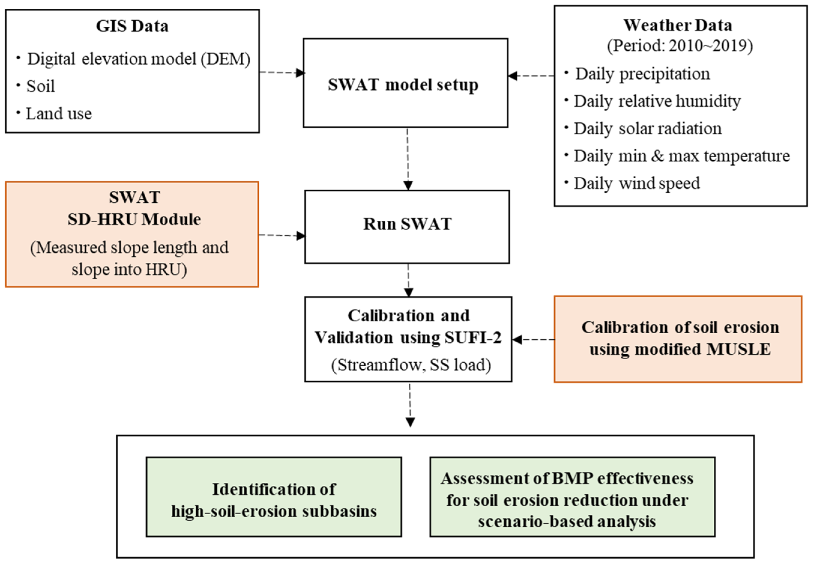
Figure 1. The procedure for evaluating BMP reduction efficiency consists of (1) applying the SD-HRU method in SWAT and adjusting it using MUSLE and (2) selecting priority management areas based on soil erosion reduction efficiency.
Agriculture 15 00893 g001
Figure 2. Locations of observation stations (M1, M2) in the Doam watershed: streamflow and SS load were monitored and used for model calibration and validation.
Agriculture 15 00893 g002
Figure 3. Input data for SWAT analysis: (a) digital elevation model (DEM), (b) soil map, (c) land use map. The soil map (b) was for soil distribution in the Doam watershed based on the detailed soil map from the Rural Development Administration (RDA) of Korea. Each color represents a distinct soil mapping unit (e.g., BANCHEON, IMOG) used in the SWAT model.
Agriculture 15 00893 g003
Figure 4. Comparison between observed and simulated streamflow at monitoring stations M1 and M2: (a) calibration period (2012–2014), (b) validation period (2015–2019).
Agriculture 15 00893 g004
Figure 5. Comparison between observed and simulated SS load at monitoring stations M1 and M2: (a) calibration period (2012–2014), (b) validation period (2015–2019).
Agriculture 15 00893 g005
Figure 6. Effectiveness of various BMPs in reducing soil erosion in subbasins of the study area.
Agriculture 15 00893 g006
Table 1. Long-term trends in annual and seasonal precipitation in the study area.
YearsAverage
Precipitation
(mm)
Seasonal (mm)
SpringSummerFallWinter
20101217.5307.2385.6397.1127.6
20111762.1304.5982.5330.0145.1
20121289.2271.7699.5223.494.6
20131052.8185.2527.4221.7118.5
20141309.6216.0586.1362.7144.8
2015982.297.2532.0296.256.8
20161183.9149.7746.0193.694.6
20171025.3110.5721.7155.038.1
20181731.0404.6854.1403.868.5
20191199.0114.0558.1507.319.6
Average1275.3216.1659.3309.190.8
Table 2. The description and the scenario settings of each BMP.
NO.DescriptionScenario 1Scenario 2
1Following marginal farmland O
2Slope reduction in high-altitude fields O
3Establishment of vegetative buffer zones in agricultural fields O
4Riparian vegetative buffer zones in stream O
5Slope protection structures (installation of NPRFs)OO
6Water channel systems (installation of NPRFs)OO
7Soil surface cover in cultivated landOO
8Distribution of onion mesh bagsOO
9Restoration of dug channelsOO
10Unauthorized cultivated landOO
Table 3. Coefficients and exponents of modified MUSLE as applied in this study.
Land UseMUSLE Runoff Factor
Existing MUSLEModified MUSLE
CoefficientExponentCoefficientExponent
Agricultural11.800.562.800.54
Forest11.800.560.380.55
Table 4. Range and optimal values of parameters used for streamflow and SS load calibration in the SWAT model.
ParametersDefinitionRangesOptimal Value
CN2SCS runoff curve number0.8–1.21.2
GWQMNThreshold depth of water in the shallow aquifer required for return flow to occur0–5000100
SOL_AWCAvailable water capacity of the soil layer0.8–1.21.2
ALPHA_BFBaseflow alpha factor0.0–1.00.183
REVAPMNThreshold depth of water in the shallow aquifer for “revap” to occur0–500200
SOL_KSaturated hydraulic conductivity (mm/h)0.8–1.21.2
SPEXPExponent parameter for calculating sediment entrained in channel sediment routing1.0–2.01.5
CH_COV2Channel cover factor−0.001–1.01.0
ADJ_PKRPeak rate adjustment factor for sediment routing in the subbasin (tributary channels)0.5–2.01.4
Table 5. Comparison of annual soil erosion and SS concentrations and their reduction efficiencies under each scenario relative to the baseline.
SectionBaselineScenario 1Scenario 2
Soil erosion2913 (tons/ha/year)1904 (34.6%)1185 (59.3%)
SS concentration 32.3 (mg/L)21.0 (35.0%)13.8 (57.3%)
Table 6. Prioritization of management areas based on soil erosion reduction efficiency through BMP implementation.
SubbasinBaselineScenario 1Scenario 2
Soil
Erosion (ton/yr)
Reduction
Efficiency (%)
Prioritization RankSoil
Erosion (ton/yr)
Reduction
Efficiency (%)
Prioritization Rank
150440819.1%1437326.0%18
298174124.5%1357641.3%14
368342537.8%836047.3%11
42052118242.4%765668.0%4
53166139655.9%297869.1%2
66038503416.6%15485219.6%22
736324033.9%919745.7%12
817714915.8%1610242.4%13
92692458.9%2121619.7%21
1089378711.9%1942652.3%9
1122511648.4%49060.0%6
1218412532.1%1112333.2%17
134624414.6%2437019.9%20
145695189.0%2025754.8%8
15211814.3%181814.3%24
16584915.5%174915.5%23
1782811.2%285335.4%16
1862642032.9%1038139.1%15
192332243.9%2517923.2%19
201906104545.2%674960.7%5
21201597351.7%387756.5%7
2240385.0%233512.5%25
2314141.4%26141.4%28
242362206.8%2221210.2%26
2515151.3%27151.3%29
26122190925.6%1238868.2%3
2763822564.7%118870.5%1
28754046.7%53652.0%10
292362350.4%292178.1%27
Disclaimer/Publisher’s Note: The statements, opinions and data contained in all publications are solely those of the individual author(s) and contributor(s) and not of MDPI and/or the editor(s). MDPI and/or the editor(s) disclaim responsibility for any injury to people or property resulting from any ideas, methods, instructions or products referred to in the content.