Smart Irrigation Scheduling for Crop Production Using a Crop Model and Improved Deep Reinforcement Learning

Abstract

In arid regions characterized by extreme water scarcity, it is important to synergistically optimize both crop yield and water use. Irrigation strategies based on empirical knowledge overlook crops’ dynamic water needs and may cause water waste and yield loss. To address this issue, this paper proposes an intelligent irrigation scheduling method based on a crop growth model and an improved deep reinforcement learning (DRL) agent. We construct a high-fidelity cotton growth environment using the Decision Support System for Agrotechnology Transfer (DSSAT) model. The model was calibrated with local data from the Shihezi region, Xinjiang, to provide a reliable simulation platform for DRL agent training. We developed a temporal state representation module based on a Bidirectional Long Short-Term Memory (BiLSTM) network and an attention mechanism. This module captures dynamic trends in historical environmental information to focus on critical decision factors. The Soft Actor–Critic (SAC) algorithm was improved by integrating a feature attention mechanism to enhance decision-making precision. A dynamic reward function was designed based on the critical growth stages of cotton to incorporate agronomic prior knowledge into the optimization objective. Simulation results demonstrate that our proposed method can improve water use efficiency (WUE) by 39.0% (with an 8.4% increase in yield and a 22.1% reduction in water consumption) compared to fixed-schedule irrigation strategies. An ablation study further confirms that each of our proposed modules—BiLSTM, the attention mechanism, and the dynamic reward—makes a significant contribution to the final performance.

1. Introduction

Water scarcity has become a core bottleneck constraining the sustainable development of global agriculture. As the world’s largest water consumer, the agricultural sector accounts for approximately 70% of all freshwater withdrawals, the majority of which is used for crop irrigation [1]. Against the backdrop of a rising global population driving continuously increasing food demand, the challenge of producing more food with limited water resources has become a pressing global issue [2]. Therefore, maximizing water use efficiency (WUE) while ensuring or even enhancing crop yields is an intrinsic requirement for modern agricultural development and a critical strategic pathway to address future water crises.

In general, crop irrigation strategies primarily encompass experience-based fixed-schedule irrigation [3] and threshold-based methods that rely on single indicators like soil moisture [4]. The core principle of these approaches is to trigger an irrigation event based on one or more easily measurable environmental indicators. The most widely applied method is the soil moisture threshold control. This technique involves deploying soil moisture sensors in the field to continuously monitor the root-zone soil water content [5,6]. When the water content falls below a preset threshold, the system initiates irrigation until it is restored to exceed the threshold [7]. This method is intuitive, easy to implement, and can, to some extent, prevent crops from suffering severe water stress. However, this is a reactive strategy that only remedies water deficits after they occur. It also overlooks future weather forecasts and the coupled effects of multiple factors like water, fertilizer, and heat [8]. Consequently, it is hard to achieve a globally optimal water allocation. Another common method is to estimate evapotranspiration from meteorological data [9,10]. This approach utilizes data from weather stations to calculate the reference evapotranspiration (ET₀) using models like the Penman–Monteith (FAO-56) equation. The actual crop evapotranspiration (ETc) is estimated by incorporating the crop coefficient (Kc), which serves as the basis for irrigation scheduling [11]. This method considers the impact of meteorological factors on crop water consumption and is generally more effective than the simple soil moisture method [12]. However, the crop coefficient (Kc) varies stagewise throughout the growing season, and its precise determination needs extensive field calibration experiments. Furthermore, this method is highly sensitive to the accuracy of meteorological data and struggles to accurately reflect local moisture variations caused by soil heterogeneity, etc.

Researchers have developed process-based crop growth models to simulate the complex processes within the soil–plant–atmosphere continuum (SPAC) [13]. These models form the core of modern irrigation decision support systems (DSSs). Most widely used systems include the Decision Support System for Agrotechnology Transfer (DSSAT) and the Agricultural Production Systems Simulator (APSIM) [14,15]. On a daily time step, they can quantitatively simulate crop growth and development, biomass accumulation, and water and nutrient balances by comprehensively analyzing meteorological conditions, soil properties, crop cultivar genetics, and management practices [16]. Researchers can conduct extensive “what-if” scenario analyses using these models: Zhao Y et al. [17] evaluated the impact of different irrigation regimes on final yield to identify a relatively optimal irrigation schedule offline. This simulation approach can search for optimal solutions across many scenarios. However, this process leads to a combinatorial explosion problem, making it too difficult for manual optimization or conventional optimization algorithms [18]. Some studies have attempted to couple crop models with optimization algorithms. Lyu et al. [19] combined the AquaCrop model with a genetic algorithm to optimize irrigation strategies under water-deficient conditions, and generated a set of optimal trade-off solutions between yield and water savings. These methods rely on offline planning before the season begins, which limits their ability to adapt to changing field conditions during the growing season.

With the advancement of sensing technologies and data science, machine learning (ML) methods have been widely applied to agricultural water resource management [20]. Researchers have utilized ML to establish predictive relationships between environmental factors and crop water requirements/soil moisture dynamics [21,22]. Goap et al. [23] employed Internet of Things (IoT) data with ML models to forecast soil moisture for irrigation purposes. These data-driven models are capable of learning nonlinear relationships from multidimensional data without in-depth knowledge of the underlying biophysical mechanisms. However, their performance highly depends on the quantity and quality of the training data, with limited generalization ability. These models are rarely used for direct sequential decision-making. Long Short-Term Memory (LSTM) networks [24] and their variants (e.g., gated recurrent unit (GRU) [25], BiLSTM [26]) have been applied to handle time-series data. Abioye et al. [27] indicate that deep learning models, especially LSTM, demonstrate excellent performance in predicting temporal variables like soil moisture. These studies primarily focus on prediction rather than decision-making.

Deep reinforcement learning (DRL) is generally designed to solve sequential decision-making problems and is a powerful theoretical framework to achieve closed-loop intelligent control [28]. Recent studies have systematically summarized the advantages, opportunities, and challenges of applying DRL to irrigation optimization [29]. DRL combines the perceptual capabilities of deep learning with the decision-making power of reinforcement learning (RL), which enables an agent to autonomously learn an optimal policy through trial-and-error interaction with its environment [30,31]. DRL has achieved significant success in industrial process control [32,33]. In agricultural irrigation, it also involves adjusting continuous control variables within a dynamic, changing environment to achieve long-term optimal system performance. Ajagekar et al. [34] utilized DRL to optimize climate control within a greenhouse, which reduced 57% energy consumption and improved control precision by over 26.8%. Chen et al. [35] applied deep Q-learning for irrigation scheduling in a simplified, hydrodynamics-based model environment, and successfully reduced irrigation water (23 mm) and optimized irrigation frequency. Saikai et al. [36] built a general framework using the APSIM model, integrating high-dimensional data to optimize irrigation rules. When such physically based models are unavailable, Alibabaei et al. [37] introduced a data-driven alternative, in which LSTM is used to build a virtual environment for DRL to increase yield by 11% and cut water use by 20–30%. Among these efforts, Liu et al. [38] developed a smart DRL-based irrigation system integrated with DSSAT and LSTM. This system increased cotton productivity by 5% and cut irrigation amounts by nearly 39%. DRL is not always efficient for irrigation management. A direct comparison by de Queiroz Pereira et al. [39] showed that when DRL maximized lettuce yield (2.5× higher than a rule-based system), the RBS was more water-efficient under scarcity. Kelly et al. [40] confirmed that DRL’s performance may not exceed other methods in normal years. Its true advantage emerges under severe physical or regulatory water scarcity, where it consistently delivers high profits. DRL is not a universal replacement, but a valuable strategic tool to manage irrigation under high-stress, constrained conditions.

Generally, the crop growth process involves interactions between uncontrolled weather factors and different crops and soils [41]. The coupled dynamics of these interactions are complex and difficult to model. To solve this problem, Gautron et al. [42] leveraged the crop simulator DSSAT to establish a modular RL environment, in which the DRL algorithm interacted with the dynamic environment to generate irrigation policies to optimize both maize yield and water use. Addressing this, Turchetta et al. [43] proposed CyclesGym, a framework based on the Cycles crop simulator that can learn multi-year policies for complex action spaces and multiple crops. It incorporates rewards and costs, and defines weather and soil generation modules to create a long-term farming RL environment. The deterministic simulation environment may cause unstable training strategies.

In this work, we develop and validate a DRL-based irrigation agent that learns within a calibrated DSSAT environment, which includes the following objectives:

(1)

Establish a high-fidelity virtual environment for DRL training by leveraging the DSSAT model, which is rigorously calibrated with local data. This environment encapsulates the intrinsic mechanisms of crop physiology and soil physics provided by the DSSAT simulator.

(2)

Develop a novel temporal state representation module. We integrate a Bidirectional Long Short-Term Memory (BiLSTM) network into the state representation module to extract hidden states for the actor’s decision-making. Furthermore, we incorporate a novel dual-attention mechanism to capture temporal dependencies and identify salient information in agricultural decision-making.

(3)

Introduce an innovative dynamic reward function contingent on the critical phenological stages of cotton in Shihezi, Xinjiang. The efficacy and superiority of the proposed framework are then systematically validated through exhaustive simulation experiments and a thorough ablation study.

2. Materials and Methods

2.1. Data Collection and Analysis

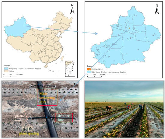
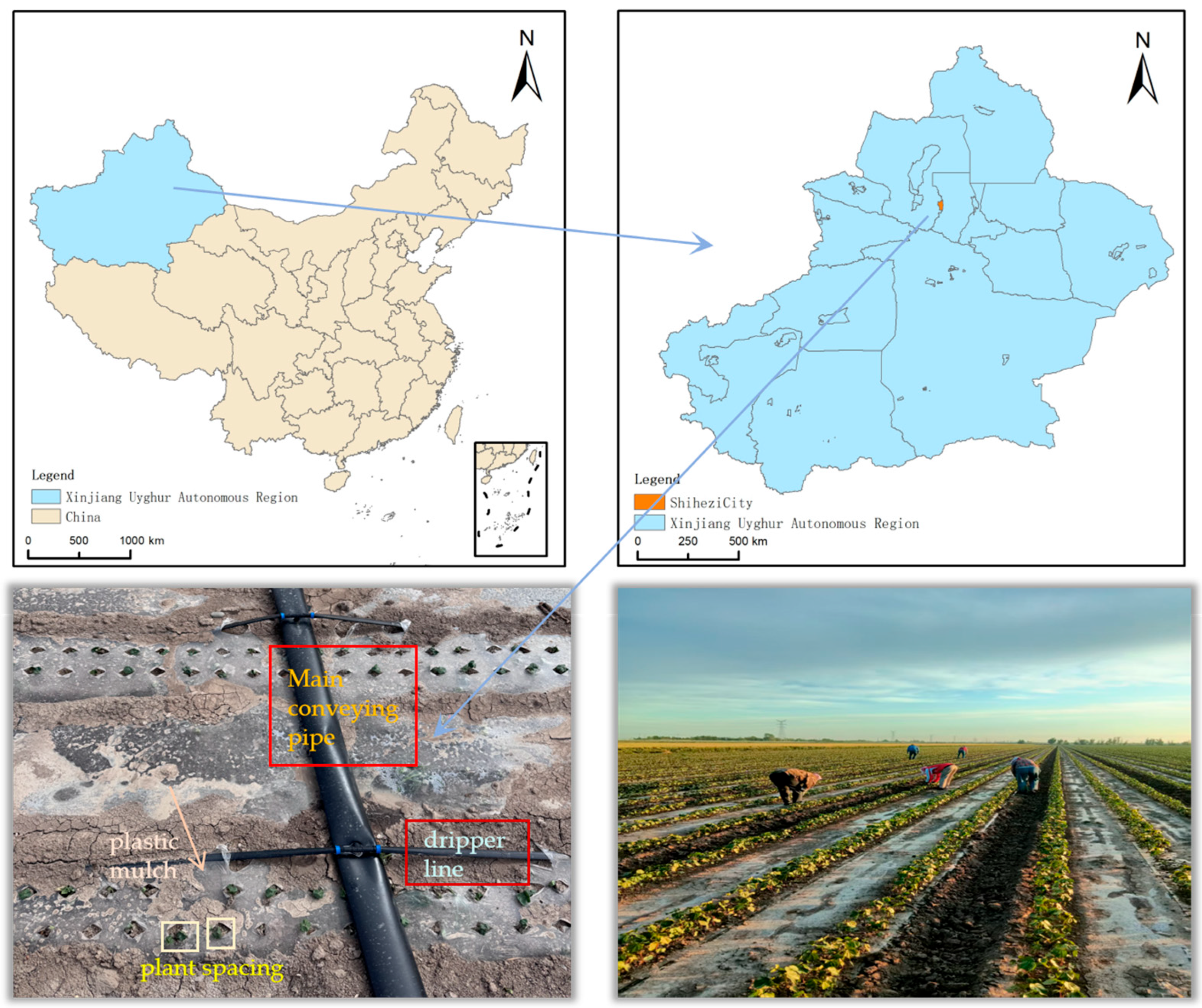
This study utilized the CSM-CROPGRO-Cotton module within DSSAT (v4.8) to simulate the cotton production process. The case study area is located in Shihezi City (44°18′ N, 85°59′ E), situated at the northern foot of the Tianshan Mountains in Xinjiang, China, with a typical continental arid climate. Cotton cultivation widely adopts a high-density and dwarf-dense-early planting pattern in the area and predominantly features drip irrigation under plastic film mulch, as illustrated in Figure 1. This technique effectively reduces surface evaporation and precisely delivers water and nutrients to the crop root zone.

Figure 1. General geographical features of the study area at Shihezi City, Xinjiang, China.

2.1.1. Meteorological Data

Daily meteorological records for the study area spanning a 10-year period from 2014 to 2024 were collected and formatted into the standard DSSAT. These records include maximum and minimum air temperature (TMAX, TMIN), precipitation (RAIN), and mean wind speed (WIND) collected from the China Meteorological Data Service Centre (http://data.cma.cn/, accessed on 18 April 2025). Solar radiation (SRAD) data were estimated using the Angstrom–Prescott model recommended by the Food and Agriculture Organization of the United Nations (FAO) [44]. This model estimates total SRAD (${\mathrm{R}}_{\mathrm{s}}$) based on the actual duration of sunshine ($\mathrm{n}$). The required inputs for the model, namely the extraterrestrial radiation (${\mathrm{R}}_{{\mathrm{s}}_0}$) and the maximum possible duration of sunshine ($\mathrm{N}$), were calculated based on the geographical latitude of the study area and the day of the year. The specific calculation formulas are as follows:

$${\mathrm{R}}_{\mathrm{s}}={\mathrm{R}}_{{\mathrm{s}}_0}\left(\mathrm{a}+\mathrm{b}{\displaystyle \frac{\mathrm{n}}{\mathrm{N}}}\right)$$

(1)

$$\mathrm{N}={\displaystyle \frac{24}{\mathsf{\pi }}}{\mathrm{w}}_{\mathrm{s}}$$

(2)

$${\mathrm{w}}_{\mathrm{s}}=\arccos \left(-\tan \left(\mathsf{\varphi }\right)\tan \left(\mathsf{\delta }\right)\right)$$

(3)

$$\mathsf{\delta }=0.409\sin \left({\displaystyle \frac{2\mathsf{\pi }}{365}}\mathrm{J}-1.39\right)$$

(4)

$${\mathrm{R}}_{{\mathrm{s}}_0}={\displaystyle \frac{24·60}{\mathsf{\pi }}}{\mathrm{G}}_{\mathrm{s}\mathrm{c}}{\mathrm{d}}_{\mathrm{r}}\left[{\mathrm{w}}_{\mathrm{s}}\sin \left(\mathsf{\varphi }\right)\sin \left(\mathsf{\delta }\right)+\cos \left(\mathsf{\varphi }\right)\cos \left(\mathsf{\delta }\right)\sin \left({\mathrm{w}}_{\mathrm{s}}\right)\right]$$

(5)

$${\mathrm{d}}_{\mathrm{r}}=1+0.033\cos \left({\displaystyle \frac{2\mathsf{\pi }}{365}}\mathrm{J}\right)$$

(6)

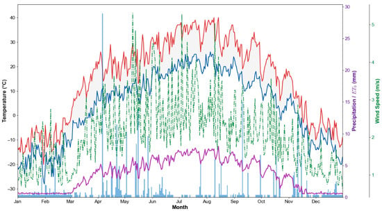
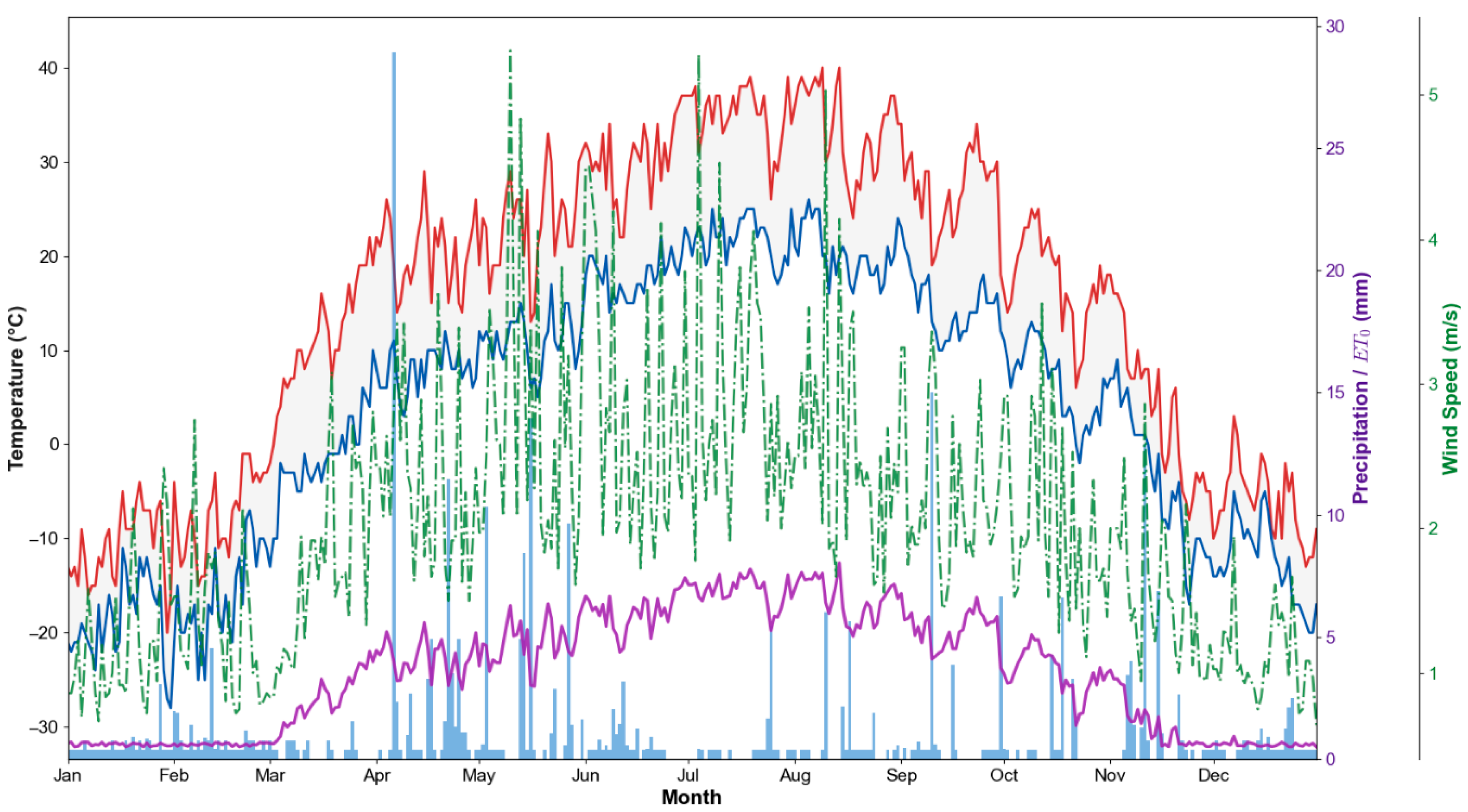
where $\mathrm{a}$ and $\mathrm{b}$ are the empirical coefficients that were set to the recommended values of 0.25 and 0.50, respectively; $\mathsf{\pi }$ equals 3.14; ${\mathrm{w}}_{\mathrm{s}}$ is the sunset hour angle; $\mathsf{\varphi }$ is the latitude, which was set to 0.773 rad corresponding to 44.3° N for Shihezi City; $\mathsf{\delta }$ is the solar declination; $\mathrm{J}$ is the day number of the year; ${\mathrm{R}}_{{\mathrm{s}}_0}$ is extraterrestrial radiation; ${\mathrm{G}}_{\mathrm{s}\mathrm{c}}$ is the solar constant, valued at 0.0820; and ${\mathrm{d}}_{\mathrm{r}}$ is the inverse relative Earth–Sun distance. Daily SRAD values were estimated and used as the output. WTH weather files required by DSSAT. The results of the time-series analysis of the key meteorological data are illustrated in Figure 2.

Figure 2. Multi-year average daily meteorological data analysis (2014–2024), in which the red line represents the average daily maximum temperature (°C), the blue line depicts the average daily minimum temperature (°C), the faint blue vertical bars indicate the average daily rainfall (mm), the purple line represents the average daily reference evapotranspiration (ETo, mm), the green dashed-dotted line shows the average daily wind speed (m/s), and the area surrounding both the red and blue temperature lines denotes the ±1 standard deviation range for the average daily temperature.

2.1.2. Soil Data

Soil samples were collected using a stratified sampling protocol and analyzed at the agricultural experimental station for cotton research of Shihezi University. The predominant soil type in this region is a Calcic Cambisol (WRB). Average parameter values of soil were calculated for each of the five-layer soil profiles extending to a depth of 120 cm and encoded into a standard DSSAT soil file (.SOL) (Table 1).

Table 1. Physicochemical properties and parameters of the soil in the study area.

Depth	Texture	Sand (%)	Silt (%)	Clay (%)	Bulk Capacity $({\mathbf{c}\mathbf{m}}^3/{\mathbf{c}\mathbf{m}}^3$)	Field Capacity $({\mathbf{c}\mathbf{m}}^3/{\mathbf{c}\mathbf{m}}^3$)	Wilting Point $({\mathbf{c}\mathbf{m}}^3/{\mathbf{c}\mathbf{m}}^3$)	Saturation $({\mathbf{c}\mathbf{m}}^3/{\mathbf{c}\mathbf{m}}^3$)	Organic Carbon (%)
SLB $(\mathrm{c}\mathrm{m}$)	-	SLSA	SLSI	SLSC	SBDM	SDUL	SLLL	SSAT	SLOC
0–20	Clay Loam	12.4	30.6	57.0	1.42	0.330	0.150	0.460	1.25
20–40	Clay Loam	14.4	26.7	58.9	1.58	0.310	0.140	0.430	1.11
40–60	Clay Loam	15.0	31.2	53.8	1.51	0.340	0.160	0.440	1.04
60–90	Clay Loam	13.7	29.8	56.5	1.50	0.350	0.175	0.435	1.05
90–120	Clay Loam	13.7	29.8	56.5	1.48	0.380	0.200	0.450	1.06

Note: The bold abbreviations in the second header row correspond to the standard variable names in the DSSAT soil file (.SOL). Field capacity (SDUL) corresponds to the water content at −33 kPa matric potential, and wilting point (SLLL) corresponds to the water content at −1500 kPa matric potential. The organic carbon content data are used for the initialization of the soil carbon module.

2.1.3. Crop Management Data

The simulated planting pattern followed a wide–narrow row configuration, with a wide row spacing of 66 cm and a narrow row spacing of 10 cm. The in-row plant spacing was set to 11 cm. The planting date was set to 15 April for each simulation year. Based on this configuration, the resulting plant density was approximately 225,000 plants per hectare. A fertilization scheme representing a medium fertility level was simulated. The total application rate of nitrogen was 240 kg/ha, and the total phosphorus application rate was 120 kg/ha. Fertilizers were applied in split applications according to a predefined nutrient demand schedule, with the specific dates and proportions detailed in Table 2.

Table 2. Field management settings for cotton in the DSSAT model.

Parameter Name	Symbol	Set Value	Description
Planting Date	PDATE	-	April 15
Row Configuration	-	cm	Wide: 66, Narrow: 10
In-row Spacing	-	cm	11
Plant Density	PLANTS	plants/ha	225,000
Total Nitrogen	-	kg/ha	240
Total Phosphorus	-	kg/ha	120
N Application 1	FDATE, FAMN	-	40 DAP, 30% of total N
N Application 2	FDATE, FAMN	-	70 DAP, 50% of total N
N Application 3	FDATE, FAMN	-	90 DAP, 20% of total N

Note: DAP refers to the number of days after sowing.

The DSSAT model was calibrated using field trial observation data from 2022 to 2024 to minimize the deviation between the model’s simulated outputs and the field-observed values. Three standard statistical metrics, root mean square error (RMSE), the coefficient of determination (${\mathrm{R}}^2$), and the normalized root mean square error ($\mathrm{n}\mathrm{R}\mathrm{M}\mathrm{S}\mathrm{E}$), were employed to quantitatively evaluate the model’s performance.

$$\mathrm{R}\mathrm{M}\mathrm{S}\mathrm{E}=\sqrt{{\displaystyle \frac{1}{\mathrm{n}}}{\sum }_{\mathrm{i}=1}^{\mathrm{n}}{\left({\mathrm{S}}_{\mathrm{i}}-{\mathrm{O}}_{\mathrm{i}}\right)}^2}$$

(7)

$${\mathrm{R}}^2=1-{\displaystyle \frac{\sum _{\mathrm{i}=1}^{\mathrm{n}}{\left({\mathrm{O}}_{\mathrm{i}}-{\mathrm{S}}_{\mathrm{i}}\right)}^2}{\sum _{\mathrm{i}=1}^{\mathrm{n}}{\left({\mathrm{O}}_{\mathrm{i}}-{\overline{\mathrm{O}}}_{\mathrm{i}}\right)}^2}}$$

(8)

$$\mathrm{n}\mathrm{R}\mathrm{M}\mathrm{S}\mathrm{E}=\sqrt{{\displaystyle \frac{{\sum _{\mathrm{i}=1}^{\mathrm{n}}\left({\mathrm{S}}_{\mathrm{i}}-{\mathrm{O}}_{\mathrm{i}}\right)}^2}{\mathrm{n}}}}/{\overline{\mathrm{O}}}_{\mathrm{i}}\times 100$$

(9)

where $\mathrm{n}$ is the number of samples; ${\mathrm{O}}_{\mathrm{i}}$ is the observed value; ${\mathrm{S}}_{\mathrm{i}}$ is the simulated value; and ${\overline{\mathrm{O}}}_{\mathrm{i}}$ is the mean of all observed values.

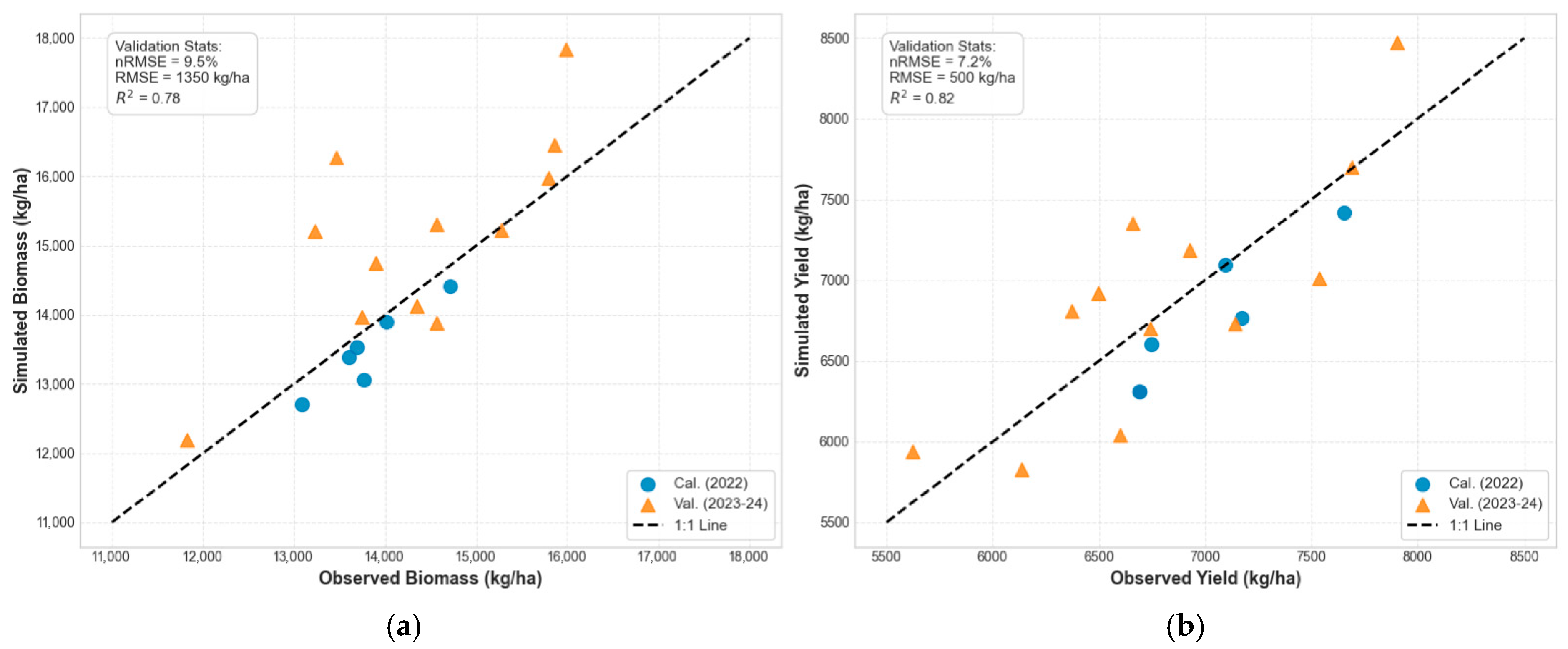
The genetic coefficients of the cotton cultivar were calibrated using field data from 2022 and validated against independent datasets from 2023 and 2024. The calibrated parameters, optimized for the local planting pattern, are listed in Table A1. Model performance was evaluated using RMSE and nRMSE. As presented in Table A2 and visualized in Figure A1, the simulation results showed good agreement with observed data. The nRMSE ranged from 3.3% to 9.5% for aboveground biomass and 3.7% to 7.2% for seed cotton yield across calibration and validation phases. These error metrics fall within the acceptable range.

2.2. Gym Environment Encapsulation

The calibrated DSSAT model was encapsulated into a Python environment, DSSAT-Gym-Env, which adheres to the OpenAI Gym interface standard. This environment facilitates interaction between the DRL agent and the DSSAT.exe engine through scripted file I/O and command-line calls. It implements core functions, including reset() and step(action). The reset() function is responsible for initializing/randomizing the simulation conditions for a growing season and returns the initial state. The step(action) function puts the irrigation action output by the agent into the appropriate DSSAT management input file to invoke the DSSAT engine to simulate a single day forward. Then, the function would parse the output files to obtain the next state and the immediate reward. The major components of the Markov decision process (MDP) can be defined as follows:

(a)

State Space ($\mathrm{S}$)

The state space is defined as ${\mathrm{s}}_{\mathrm{t}}$ = [LAI, CWAD, RTDP, GSTD, SWAD, SWFAC, TMAX, TMIN, SRAD, RAIN, WIND]. The rationale for selecting these specific variables is to capture the complete dynamics of the soil–plant–atmosphere system, which governs crop water balance. Meteorological variables (TMAX, TMIN, SRAD, WIND, and RAIN) are included to capture the atmospheric evaporative demand. Leaf area index (LAI) and aboveground dry matter (CWAD, kg/ha) quantify the transpiration surface and biomass accumulation; Root depth (RTDP, cm) defines the effective soil water extraction zone; and growth stage code (GSTD) indicates phenological phases with varying water sensitivity. Soil water in the available depth (SWAD, mm) reflects the root-zone water supply capability. The water stress factor (SWFAC) is an index ranging from 0 to 1, where 0 represents sufficient water and 1 represents a complete cessation of photosynthesis due to water deficit. Furthermore, the relevance of these features is dynamically evaluated by the attention mechanism, analyzed in Section 3.3.

(b)

Action Space ($\mathrm{A}$)

The action (${\mathrm{a}}_{\mathrm{t}}$) is defined as the amount of irrigation water applied on a given decision day ($\mathrm{t}$). It is a bounded, one-dimensional continuous space, designed to match the capabilities of modern precision irrigation systems:

$${\mathrm{a}}_{\mathrm{t}}\in \left[0,{\mathrm{I}}_{\mathrm{m}\mathrm{a}\mathrm{x}}\right]$$

(10)

where ${\mathrm{I}}_{\mathrm{m}\mathrm{a}\mathrm{x}}$ is set to 60 mm, representing the daily maximum water delivery capacity of the irrigation system. To ensure physical feasibility, the raw output of the actor network is constrained using a tanh activation function, mapping values to [−1, 1], which are then linearly scaled to the valid range [0, ${\mathrm{I}}_{\mathrm{m}\mathrm{a}\mathrm{x}}$]. This mechanism prevents the selection of negative or excessive irrigation amounts. Furthermore, while the algorithm operates in a continuous space, the execution resolution is physically limited to 0.1 mm to match the precision of the drip irrigation system. It is important to emphasize that the output of the agent action represents the total irrigation quota for the decision day. In this work, a drip irrigation system under plastic film mulch was applied to irrigate the crop root zone.

(c)

Dynamic Reward Function ($\mathrm{R}$)

The reward function ($\mathrm{R}$) provides the learning signal to optimize the agent’s policy. A composite reward function with dynamically adjusted weights was developed to enable the agent to learn complex trade-offs that vary with the crop’s phenological stage. At each time step ($\mathrm{t}+1$), the immediate reward (${\mathrm{R}}_{\mathrm{t}}$) is calculated based on the new state (${\mathrm{s}}_{\mathrm{t}+1}$) and the action (${\mathrm{a}}_{\mathrm{t}}$) taken at the previous step:

$${\mathrm{R}}_{\mathrm{t}}={\mathrm{w}}_{\mathrm{y}}\left({\mathrm{G}}_{\mathrm{t}+1}\right){\mathrm{r}}_{\mathrm{y}}-{\mathrm{w}}_{\mathrm{w}}\left({\mathrm{G}}_{\mathrm{t}+1}\right){\mathrm{r}}_{\mathrm{w}}-{\mathrm{w}}_{\mathrm{s}}\left({\mathrm{G}}_{\mathrm{t}+1}\right){\mathrm{r}}_{\mathrm{s}}$$

(11)

$${\mathrm{r}}_{\mathrm{y}}=∆{\mathrm{C}\mathrm{W}\mathrm{A}\mathrm{D}}_{\mathrm{t}}={\mathrm{C}\mathrm{W}\mathrm{A}\mathrm{D}}_{\mathrm{t}+1}-{\mathrm{C}\mathrm{W}\mathrm{A}\mathrm{D}}_{\mathrm{t}}$$

(12)

where ${\mathrm{r}}_{\mathrm{y}}$ is the yield gain term that rewards effective crop growth; ${\mathrm{r}}_{\mathrm{w}}$ is the water consumption cost term, which equals the daily irrigation amount (${\mathrm{a}}_{\mathrm{t}}$); and ${\mathrm{r}}_{\mathrm{s}}$ is the water stress penalty term, calculated as the square of the water stress factor to severely penalize any action that leads to crop water stress; ${\mathrm{G}}_{\mathrm{t}+1}$ is the current crop growth stage, which is determined by the GSTD within the state vector ${\mathrm{S}}_{\mathrm{t}+1}$; and ${\mathrm{w}}_{\mathrm{y}}$, ${\mathrm{w}}_{\mathrm{w}}$, and ${\mathrm{w}}_{\mathrm{s}}$ are the dynamic weights, which are functions of ${\mathrm{G}}_{\mathrm{t}+1}$. By using the square of the SWFAC, we apply a nonlinear, amplified penalty for deviations from the ideal stress-free state (SWFAC = 0). $∆{\mathrm{C}\mathrm{W}\mathrm{A}\mathrm{D}}_{\mathrm{t}}$ directly quantifies the daily increase in biomass.

We divided the entire cotton growing season into five critical stages and predefined an optimized set of weights for each stage. The specific weight function W(G) is defined in Table 3. When the seedlings emerge from the soil, the stress weight ${\mathrm{w}}_{\mathrm{s}}$ is set to 1.5 to ensure seedling survival. In the squaring stage, ${\mathrm{w}}_{\mathrm{y}}$ and ${\mathrm{w}}_{\mathrm{s}}$ are increased to prevent bud shedding caused by water stress. In the flowering and boll-setting stage, ${\mathrm{w}}_{\mathrm{s}}$ is set high to prevent substantial flower and boll shedding. In the boll-opening stage, the crop’s water demand decreases, so ${\mathrm{w}}_{\mathrm{w}}$ is increased, and both ${\mathrm{w}}_{\mathrm{y}}$ and ${\mathrm{w}}_{\mathrm{s}}$ are reduced for water control. In the maturity period, irrigation is ceased by setting the ${\mathrm{w}}_{\mathrm{w}}$ to a very high value of 1.5.

Table 3. Dynamic weight configuration for the reward function across different critical growth stages of cotton.

Growth Stage	Yield Gain Weight (${\mathbf{w}}_{\mathbf{y}}$)	Irrigation Cost Weight (${\mathit{w}}_{\mathit{w}}$)	Water Stress Weight (${\mathit{w}}_{\mathit{s}}$)
Seedling Emergence	0.8	0.5	1.5
Squaring	1.0	0.3	2.0
Flowering and Boll-setting	1.2	0.1	3.5
Boll Opening	0.5	1.0	1.0
Maturity	0.1	1.5	0.5

2.3. Improved Design of Deep Reinforcement Learning Agents

2.3.1. State Representation Preprocessing

The evapotranspiration (ET₀) provides a comprehensive representation of the atmospheric evaporative demand for the day. It can be used to replace the multiple original meteorological variables. The reference ET₀ was calculated using the Penman–Monteith method:

$${\mathrm{E}\mathrm{T}}_0={\displaystyle \frac{0.408∆({\mathrm{R}}_{\mathrm{n}}-\mathrm{G})+\mathsf{\gamma }\frac{900}{\mathrm{T}+273}{\mathrm{u}}_2({\mathrm{e}}_{\mathrm{s}}-{\mathrm{e}}_{\mathrm{a}})}{∆+\mathsf{\gamma }(1+0.34{\mathrm{u}}_2)}}$$

(13)

where $∆$ is the slope of the saturation vapor pressure curve; ${\mathrm{R}}_{\mathrm{n}}$ is the net radiation at the crop surface; $\mathrm{G}$ is the soil heat flux density; $\mathsf{\gamma }$ is the psychrometric constant; $\mathrm{T}$ is the mean daily air temperature; ${\mathrm{e}}_{\mathrm{s}}$ and ${\mathrm{e}}_{\mathrm{a}}$ are the saturation and actual vapor pressures, respectively; ${\mathrm{u}}_2$ is the wind speed at 2 m above the ground surface. All intermediate variables were calculated following the standardized procedures outlined in FAO-56. One-Hot Encoding was applied for the categorical feature GSTD. All continuous numerical features in the state vector were normalized within [0, 1] after completing the feature engineering ${\mathrm{s}}^{\prime }$ (Equation (14)).

$${\mathrm{s}}^{\prime }={\displaystyle \frac{\mathrm{s}-{\mathrm{s}}_{\mathrm{m}\mathrm{i}\mathrm{n}}}{{\mathrm{s}}_{\mathrm{m}\mathrm{a}\mathrm{x}}-{\mathrm{s}}_{\mathrm{m}\mathrm{i}\mathrm{n}}}}$$

(14)

where $\mathrm{s}$ is the original feature value; ${\mathrm{s}}_{\mathrm{m}\mathrm{i}\mathrm{n}}$ and ${\mathrm{s}}_{\mathrm{m}\mathrm{a}\mathrm{x}}$ are the global minimum and maximum values for that feature across the entire dataset. Through this process, the original 11-dimensional state vector was transformed into a 12-dimensional preprocessed state vector ${\mathrm{s}}_{\mathrm{t}}^{\prime }$. Specifically, the 12 dimensions result from replacing 4 meteorological variables (TMAX, TMIN, SRAD, WIND) with ET₀, retaining RAIN, and expanding GSTD into 5 One-Hot features.

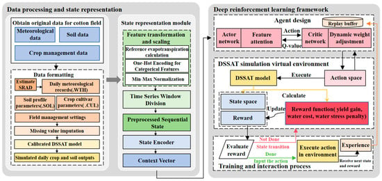
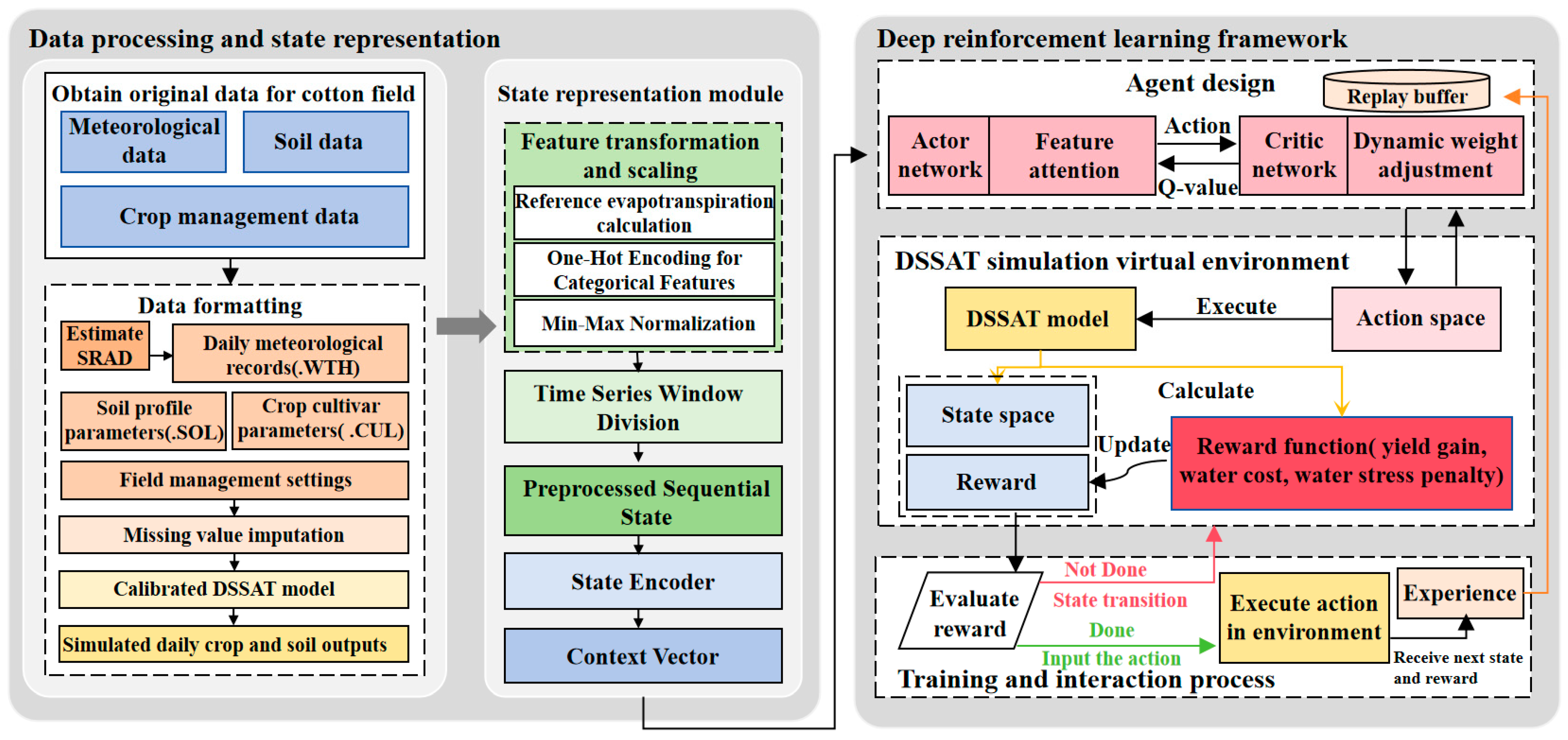
An improved Soft Actor–Critic agent featuring temporal awareness and a dual-attention mechanism (Temporal–Spatial Attention Soft Actor–Critic, TSA-SAC) was developed to learn the optimal irrigation policy within the DSSAT virtual environment. The architecture of TSA-SAC consists of an improved agent, a DSSAT-driven environment, and a replay buffer (Figure 3). The agent continuously learns and generates superior irrigation scheduling policies by interacting persistently with the environment. The environment updates the crop and soil states based on the agent’s irrigation decisions and returns a corresponding reward. The series of experiences generated during this interaction is stored in the replay buffer, structured as sequential states. An experience replay mechanism is used to train and update the actor and critic networks by randomly sampling mini-batches of these experiences. The TSA-SAC agent is composed of a perception module and a decision-making module.

Figure 3. Framework design of TSA-SAC.

2.3.2. Perception Module

Irrigation scheduling inherently exhibits a partially observable Markov property (POMDP). An optimal irrigation decision depends not only on the current soil moisture but also on the historical context. A state representation module was developed to transform a sequence of instantaneous states into a context vector that contains dynamic trends and critical historical information. This module is primarily composed of two cascaded components: (1) a temporal feature extraction network based on a Bidirectional Long Short-Term Memory (BiLSTM) network, which is used to capture long-term dependencies within the state sequence, and (2) a context aggregation network based on an attention mechanism, which is used to dynamically weigh the importance of different historical time steps.

At each decision step ($\mathrm{t}$), we constructed a sequential state matrix (${\mathrm{S}}_{\mathrm{t}}$) by storing the preprocessed state vectors in a time window of length $\mathrm{L}$. To determine the optimal time window length for the BiLSTM module, we conducted a sensitivity analysis testing values of 3, 5, 7, 10, and 14 days. The experimental results demonstrated that the model achieved its optimal performance when the time window was set to 7 days. Shorter windows failed to capture sufficient temporal context, while longer windows introduced noise and increased training difficulty without improving yield. Consequently, L = 7 was selected as the default setting for all subsequent experiments.

$${\mathrm{S}}_{\mathrm{t}}=\left[\begin{array}{c}\begin{array}{c}{\mathrm{s}}_1^{\prime }\\ {\mathrm{s}}_2^{\prime }\end{array}\\ ⋮\\ {\mathrm{s}}_{\mathrm{L}}^{\prime }\end{array}\right]\in {\mathbb{R}}^{\mathrm{L}\times \mathrm{d}}$$

(15)

where the sequence length $\mathrm{L}$ is set to 7, and $\mathrm{d}$ is the state vector dimension. ${\mathrm{s}}_1^{\prime }$, ${\mathrm{s}}_2^{\prime }$, …, ${\mathrm{s}}_{\mathrm{L}}^{\prime }$ represent individual preprocessed state vectors at different time steps within a time window of length L. We designed a stacked BiLSTM architecture with two layers, and a dropout layer (rate = 0.2) was inserted between the LSTM layers to prevent overfitting. The BiLSTM processes the input sequence ${\mathrm{S}}_{\mathrm{t}}$ to generate a sequence of hidden states ${\mathrm{H}}_{\mathrm{t}}={\left({\mathrm{h}}_1,\dots ,{\mathrm{h}}_{\mathrm{L}}\right)}^{\mathrm{T}}$, where each ${\mathrm{h}}_{\mathrm{k}}$ is a concatenation of forward and backward LSTM hidden states.

$${\mathrm{h}}_{\mathrm{k}}=\left[{\mathrm{L}\mathrm{S}\mathrm{T}\mathrm{M}}_{\mathrm{f}}({\mathrm{s}}_{\mathrm{k}},{\mathrm{h}}_{\mathrm{f}}(\mathrm{k}-1\left)\right);{\mathrm{L}\mathrm{S}\mathrm{T}\mathrm{M}}_{\mathrm{b}}({\mathrm{s}}_{\mathrm{k}},{\mathrm{h}}_{\mathrm{b}}(\mathrm{k}-1\left)\right)\right]$$

(16)

$${\mathrm{e}}_{\mathrm{k}}={\mathrm{u}}_{\mathrm{w}}^{\mathrm{T}}\mathrm{t}\mathrm{a}\mathrm{n}\mathrm{h}({\mathrm{W}}_{\mathrm{h}}·{\mathrm{h}}_{\mathrm{k}}+{\mathrm{b}}_{\mathrm{h}})$$

(17)

where ${\mathrm{e}}_{\mathrm{k}}$ is a scalar attention score; ${\mathrm{W}}_{\mathrm{h}}$, ${\mathrm{b}}_{\mathrm{h}}$, and ${\mathrm{u}}_{\mathrm{w}}$ are the learnable parameters of a fully connected attention network. These scores are then normalized via a $\mathrm{s}\mathrm{o}\mathrm{f}\mathrm{t}\mathrm{m}\mathrm{a}\mathrm{x}$ function to produce attention weights. The final context vector ${\mathrm{c}}_{\mathrm{t}}$ is computed as the attention-weighted sum of the hidden states.

$${\mathrm{c}}_{\mathrm{t}}={\sum }_{\mathrm{k}=1}^{\mathrm{L}}\mathrm{s}\mathrm{o}\mathrm{f}\mathrm{t}\mathrm{m}\mathrm{a}\mathrm{x}{\left(\mathrm{e}\right)}_{\mathrm{k}}·{\mathrm{h}}_{\mathrm{k}}$$

(18)

where $\mathrm{s}\mathrm{o}\mathrm{f}\mathrm{t}\mathrm{m}\mathrm{a}\mathrm{x}{\left(\mathrm{e}\right)}_{\mathrm{k}}$ represents the element of the weight vector, which is obtained by applying the $\mathrm{s}\mathrm{o}\mathrm{f}\mathrm{t}\mathrm{m}\mathrm{a}\mathrm{x}$ function to the entire score vector $\mathrm{e}$. The parameters of the state encoder are updated driven by the SAC decision-making task.

2.3.3. Decision-Making Module

Soft Actor–Critic (SAC) [45] is an off-policy deep reinforcement learning algorithm for continuous action spaces, which includes one Actor network and two Critic networks. The Actor network is the policy network, which calculates the current action based on the current state. The Critic network is the evaluation network, which measures the quality of a state–action pair ${(\mathrm{s}}_{\mathrm{t}},{\mathrm{a}}_{\mathrm{t}})$. The optimization objective of the SAC agent is to seek a target policy that maximizes both the return and the entropy.

$$\mathrm{J}\left(\mathsf{\theta }\right)={\mathbb{E}}_{\mathsf{\tau }~{\mathsf{\pi }}_{\mathsf{\theta }}}\left[{\sum }_{\mathrm{t}=0}^{\mathrm{T}}{\mathsf{\gamma }}^{\mathrm{t}}\left(\mathrm{r}\left({\mathrm{s}}_{\mathrm{t}},{\mathrm{a}}_{\mathrm{t}}\right)+\mathsf{\alpha }\mathrm{H}\left({\mathsf{\pi }}_{\mathsf{\theta }}(·\left|{\mathrm{s}}_{\mathrm{t}}\right.\right)\right)\right]$$

(19)

where ${\mathsf{\pi }}_{\mathsf{\theta }}$ is the policy network; $\mathsf{\theta }$ is the parameter of the policy network; $\mathsf{\tau }$ is the trajectory generated by the interaction between the policy ${\mathsf{\pi }}_{\mathsf{\theta }}$ and the environment; ${\mathbb{E}}_{\mathsf{\tau }~{\mathsf{\pi }}_{\mathsf{\theta }}}$ represents taking the expectation over trajectories generated by the policy ${\mathsf{\pi }}_{\mathsf{\theta }}$; $\mathrm{T}$ represents the maximum time step of a complete episode; $\mathsf{\gamma }$ is the discount factor, and $\mathsf{\gamma }$ $\in \left[\mathrm{0,1}\right]$ balances the relative importance of immediate and future rewards, with its value determined through hyperparameter search; $\mathrm{r}\left({\mathrm{s}}_{\mathrm{t}},{\mathrm{a}}_{\mathrm{t}}\right)$ is the immediate reward obtained by executing action ${\mathrm{a}}_{\mathrm{t}}$ in state ${\mathrm{s}}_{\mathrm{t}}$; $\mathrm{H}\left({\mathsf{\pi }}_{\mathsf{\theta }}(·\left|{\mathrm{s}}_{\mathrm{t}}\right.\right)$ is the entropy of the policy in state ${\mathrm{s}}_{\mathrm{t}}$; and $\mathsf{\alpha }$ is the temperature parameter, which balances the relative importance of the reward return and the policy entropy.

On this basis, we embed a Feature Attention Module inside the Actor network.

$${\mathrm{c}}_{\mathrm{t}}^{\prime }={\mathsf{\beta }}_{\mathrm{t}}\odot {\mathrm{c}}_{\mathrm{t}}$$

(20)

$${\mathsf{\beta }}_{\mathrm{t}}=\mathrm{s}\mathrm{o}\mathrm{f}\mathrm{t}\mathrm{m}\mathrm{a}\mathrm{x}\left({\mathrm{W}}_{{\mathrm{f}}_2}·\mathrm{R}\mathrm{e}\mathrm{L}\mathrm{U}({\mathrm{W}}_{{\mathrm{f}}_1}·{\mathrm{c}}_{\mathrm{t}}+{\mathrm{b}}_{{\mathrm{f}}_1}\right)+{\mathrm{b}}_{{\mathrm{f}}_2})$$

(21)

where ${\mathrm{c}}_{\mathrm{t}}^{\prime }$ is the state representation after feature attention weighting; ${\mathsf{\beta }}_{\mathrm{t}}$ is the feature attention weight; $\odot$ is the Hadamard product; and ${\mathrm{W}}_{{\mathrm{f}}_1}$, ${\mathrm{b}}_{{\mathrm{f}}_1}$, ${\mathrm{W}}_{{\mathrm{f}}_2}$ and ${\mathrm{b}}_{{\mathrm{f}}_2}$ are learnable parameters.

The construction and execution process of the TSA-SAC agent includes the following steps:

Step 1:

The state representation ${\mathrm{c}}_{\mathrm{t}}^{\prime }$ weighted by feature attention is mapped to an optimal irrigation action in the Actor network. The network’s output layer is divided into two separate heads, which predict the mean ${\mathsf{\mu }}_{\mathsf{\theta }}\left({\mathrm{c}}_{\mathrm{t}}^{\prime }\right)$ and the log standard deviation ${\mathrm{l}\mathrm{o}\mathrm{g}\mathsf{\sigma }}_{\mathsf{\theta }}\left({\mathrm{c}}_{\mathrm{t}}^{\prime }\right)$ of a Gaussian distribution, respectively. The action is then sampled from this distribution using the reparameterization trick.

$${\mathrm{a}}_{\mathrm{t}}=\mathrm{t}\mathrm{a}\mathrm{n}\mathrm{h}\left({\mathsf{\mu }}_{\mathsf{\theta }}\right({\mathrm{c}}_{\mathrm{t}}^{\prime })+{\mathsf{\sigma }}_{\mathsf{\theta }}({\mathrm{c}}_{\mathrm{t}}^{\prime })\odot \mathsf{\epsilon })$$

(22)

where $\mathsf{\epsilon }$ is random noise sampled from a standard normal distribution. The $\mathrm{t}\mathrm{a}\mathrm{n}\mathrm{h}$ function is used to squash the action into the [−1, 1] interval, ensuring the action is bounded.

Step 2:

The corresponding Q-value for taking action ${\mathrm{a}}_{\mathrm{t}}$ in the context state ${\mathrm{c}}_{\mathrm{t}}$ is evaluated in two independent Critic evaluation networks ${\mathrm{Q}}_{{\mathsf{\varphi }}_1}$ and ${\mathrm{Q}}_{{\mathsf{\varphi }}_2}$, with parameters ${\mathsf{\varphi }}_1$ and ${\mathsf{\varphi }}_2$ respectively. Since both the state ${\mathrm{s}}_{\mathrm{t}}$ and the context ${\mathrm{c}}_{\mathrm{t}}$ are temporally dependent, the computed Q-value also reflects the long-term value of this sequential state-action pair.

Step 3:

The target Critic networks ${\mathrm{Q}}_{{\mathsf{\varphi }}_1^{\prime }}^{\prime }$ and ${\mathrm{Q}}_{{\mathsf{\varphi }}_2^{\prime }}^{\prime }$, with parameters ${\mathsf{\varphi }}_1^{\prime }$ and ${\mathsf{\varphi }}_2^{\prime }$, are delayed copies of the evaluation network parameters. They are used to compute the Temporal-Difference (TD) Target ${\mathrm{y}}_{\mathrm{t}}$. The smaller of the two target Q-network outputs is used in the calculation to mitigate value overestimation resulting from function approximation errors.

$${\mathrm{y}}_{\mathrm{t}}={\mathrm{r}}_{\mathrm{t}}+\mathsf{\gamma }\mathrm{\ast } (1-\mathrm{d})(\underset{\mathrm{j}=\mathrm{1,2}}{\min } {\mathrm{Q}}_{{\mathsf{\varphi }}_{\mathrm{j}}}^{\prime }({\mathrm{c}}_{\mathrm{t}+1}^{\prime },{\mathrm{a}}_{\mathrm{t}+1}^{\prime })-\mathsf{\alpha }{\log }_{{\mathsf{\pi }}_{\mathsf{\theta }}}({\mathrm{a}}_{\mathrm{t}+1}^{\prime }\left|{\mathrm{c}}_{\mathrm{t}+1}))\right.$$

(23)

where d is a flag indicating the end of an episode, and ${\mathrm{a}}_{\mathrm{t}+1}^{\prime }$ is a new action sampled from the current policy for the next state ${\mathrm{c}}_{\mathrm{t}+1}$.

Step 4:

A mini-batch of data is sampled from the experience replay buffer D. The parameters of the Critic networks ${\mathsf{\varphi }}_{\mathrm{i}}$ are updated by minimizing the MSE of the soft Bellman residual.

$$\mathrm{L}\left({\mathsf{\varphi }}_{\mathrm{i}}\right)={\mathbb{E}}_{({\mathrm{c}}_{\mathrm{t}},{\mathrm{a}}_{\mathrm{t}},{\mathrm{r}}_{\mathrm{t}},{\mathrm{c}}_{\mathrm{t}+1})~\mathrm{D}}\left[{{(\mathrm{Q}}_{{\mathsf{\varphi }}_{\mathrm{i}}}({\mathrm{c}}_{\mathrm{t}},{\mathrm{a}}_{\mathrm{t}})-{\mathrm{y}}_{\mathrm{t}})}^2\right],\mathrm{f}\mathrm{o}\mathrm{r} \mathrm{i}=\mathrm{1,2}$$

(24)

The goal of the Actor network is to maximize the weighted sum of the policy’s expected return and its entropy. Its parameters $\mathsf{\theta }$ and the parameters of the perception module ${\mathsf{\Theta }}_{\mathrm{E}}$ are jointly updated using the Policy Gradient.

$$\mathrm{L}\left(\mathsf{\theta },{\mathsf{\Theta }}_{\mathrm{E}}\right)={\mathbb{E}}_{{\mathrm{S}}_{\mathrm{t}}~\mathrm{D},{\mathrm{a}}_{\mathrm{t}}~{\mathsf{\pi }}_{\mathsf{\theta }}}\left[\mathsf{\alpha }{\log }_{{\mathsf{\pi }}_{\mathsf{\theta }}}\left({\mathrm{a}}_{\mathrm{t}}\left|{\mathrm{f}}_{\mathrm{E}}({\mathrm{S}}_{\mathrm{t}};{\mathsf{\Theta }}_{\mathrm{E}})\right.\right)-\underset{\mathrm{j}=\mathrm{1,2}}{\min } {\mathrm{Q}}_{{\mathsf{\varphi }}_{\mathrm{j}}}\left({\mathrm{f}}_{\mathrm{E}}\right({\mathrm{S}}_{\mathrm{t}};{\mathsf{\Theta }}_{\mathrm{E}}),{\mathrm{a}}_{\mathrm{t}})\right]$$

(25)

where ${\mathsf{\Theta }}_{\mathrm{E}}$ is the set of learnable parameters for the state encoder. When computing the gradient, the parameters of ${\mathrm{Q}}_{{\mathsf{\varphi }}_{\mathrm{j}}}$ are treated as constants. The entropy temperature coefficient $\mathsf{\alpha }$ is automatically updated by minimizing its loss function $\mathrm{L}\left(\mathsf{\alpha }\right)$:

$$\mathrm{L}\left(\mathsf{\alpha }\right)={\mathbb{E}}_{{\mathrm{a}}_{\mathrm{t}}~{\mathsf{\pi }}_{\mathsf{\theta }}}\left[-\mathsf{\alpha }({\log }_{{\mathsf{\pi }}_{\mathsf{\theta }}}\left({\mathrm{a}}_{\mathrm{t}}\left|{\mathrm{c}}_{\mathrm{t}}\right.\right)+\overline{\mathrm{H}}\right]$$

(26)

where $\overline{\mathrm{H}}$ is the target entropy, typically set to the negative of the action space dimension. As the irrigation decision task in this study is a one-dimensional continuous action space, we set $\overline{\mathrm{H}}$ to −1. Adam optimizer is used for gradient descent to update ${\mathsf{\varphi }}_1$, ${\mathsf{\varphi }}_2$, $\mathsf{\theta }$, ${\mathsf{\Theta }}_{\mathrm{E}}$, and $\mathsf{\alpha }$.

Step 5:

Parameters are slowly copied from the evaluation networks to the target networks periodically via a soft update. The target network parameters are updated online using an update coefficient $\mathsf{\tau }$.

$${\mathsf{\varphi }}_{\mathrm{i}}^{\prime }\leftarrow \mathsf{\tau }\mathrm{\ast } \mathsf{\varphi }+\left(1-\mathsf{\tau }\right) \mathrm{\ast } {\mathsf{\varphi }}_{\mathrm{i}}^{\prime },\mathrm{f}\mathrm{o}\mathrm{r} \mathrm{i}=\mathrm{1,2}$$

(27)

where $\mathsf{\tau }$ is a small update coefficient, set to 0.005.

Step 6:

The process returns to Step 1 using the new sequential state as input for the next decision to create an iterative loop. The agent continuously repeats the perception–decision–execution–learning cycle until the entire growing season is complete. The optimized irrigation policy network ${\mathsf{\pi }}^{\mathrm{*}}$ is the output when finishing all training episodes (Algorithm 1).

Algorithm 1: TSA-SAC Algorithm

Input: The capacity of the replay buffer $\mathrm{B}$, mini-batch size $\mathrm{N}$, sequence length $\mathrm{L}$, discount factor $\mathsf{\gamma }$, the learning rate of encoder network ${\mathsf{\vartheta }}^{\mathrm{E}}$, the learning rate of actor network ${\mathsf{\vartheta }}^{\mathrm{A}}$, the learning rate of critic network ${\mathsf{\vartheta }}^{\mathrm{C}}$, soft update parameter $\mathsf{\tau }$. I Initialization: Replay buffer $\mathrm{D}$; The training environment env = DSSAT_Gym_Env( ); The state encoder network, the actor evaluation network, the critic evaluation network and parameters of them ${\mathsf{\Theta }}_{\mathrm{E}}$, $\mathsf{\theta }$, ${\mathsf{\varphi }}_1$, ${\mathsf{\varphi }}_2$; The critic target network and parameters of them ${\mathsf{\varphi }}_1^{\prime }$, ${\mathsf{\varphi }}_2^{\prime }$; The entropy temperature parameter $\mathsf{\alpha }$. II Training model:  for episode $=1$, N do   randomly initialize the initial sequential state ${\mathrm{S}}_1$   for steps $=1$, T do    Input state into encode sequential network, and calculate action ${\mathrm{a}}_{\mathrm{t}}$ according to current context vector    Execute action ${\mathrm{a}}_{\mathrm{t}}$ in virtual environment, getting the reward ${\mathrm{r}}_{\mathrm{t}}$ and next sequential state ${\mathrm{S}}_{\mathrm{t}+1}$    Store experiences $\left({\mathrm{S}}_{\mathrm{t}}, {\mathrm{a}}_{\mathrm{t}}, {\mathrm{r}}_{\mathrm{t}}, {\mathrm{S}}_{\mathrm{t}+1}\right)$ in the replay buffer $\mathrm{D}$    If len(D) > $\mathrm{N}$     Sample a random batch of experiences (${\mathrm{S}}_{\mathrm{j}}$, ${\mathrm{a}}_{\mathrm{j}}$, ${\mathrm{r}}_{\mathrm{j}}$, ${\mathrm{S}}_{\mathrm{j}+1}$)     Calculate target Q value ${\mathrm{y}}_{\mathrm{j}}$     Update the critic evaluation network parameter ${\mathsf{\varphi }}_{\mathrm{i}}$ from Equation (24)     Update the actor evaluation network parameter and the state encoder network parameter ${\mathsf{\Theta }}_{\mathrm{E}}$ from Equation (25)     Update the entropy temperature parameter $\mathsf{\alpha }$ from Equation (26)     Soft-update the target critic network: ${\mathsf{\varphi }}_{\mathrm{i}}^{\prime }\leftarrow \mathsf{\tau } \ast \mathsf{\varphi } + \left(1 - \mathsf{\tau }\right) \ast {\mathsf{\varphi }}_{\mathrm{i}}^{\prime }, \mathrm{for} \mathrm{i} = 1,2$    end if   end for  end for

2.4. Experimental Design and Evaluation Indicators

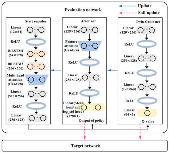
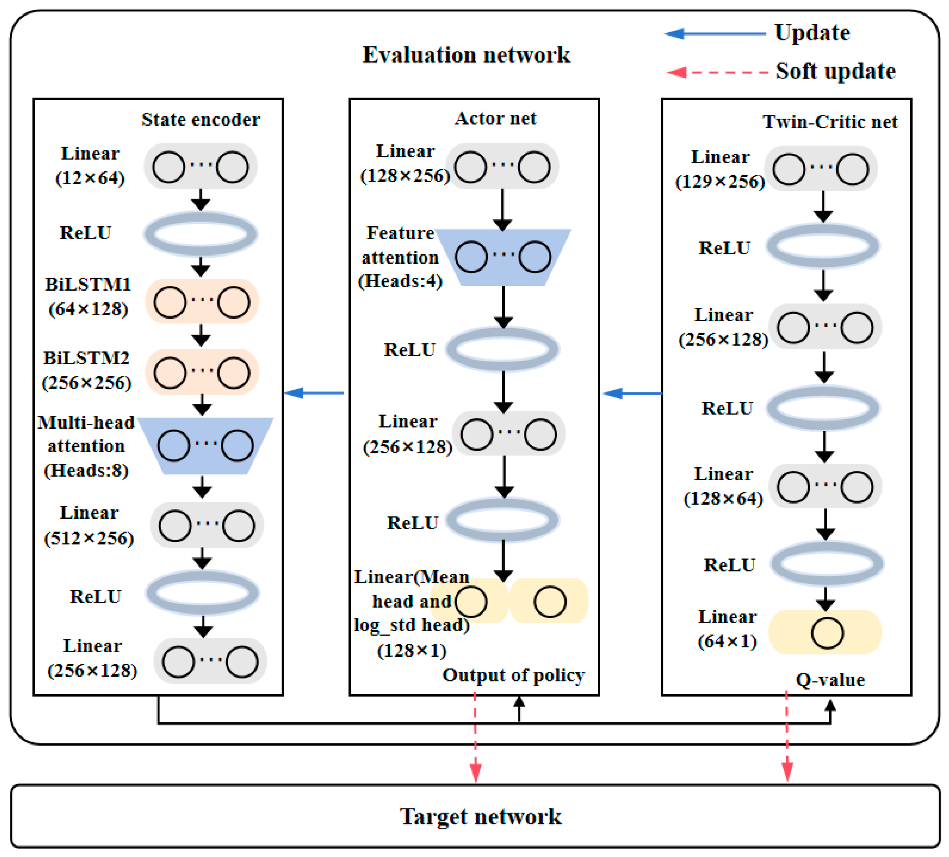
The TSA-SAC agent and all the benchmark models were implemented based on the PyTorch framework (Figure 4). Bayesian optimization [46] was used to conduct an initial exploration of the parameters to quickly locate the parameter regions with better performance. In the vicinity of the optimal region found by Bayesian optimization, we adopted the traditional grid search [47] to conduct exhaustive tuning of the key parameters such as batch size N and time window length L (Table 4).

Figure 4. Detailed neural network architecture of the TSA-SAC agent.

Table 4. Core hyperparameter configuration for the TSA-SAC agent.

Parameter Name	Symbol	Value
Learning rate (Actor)	${\mathsf{\vartheta }}^{\mathrm{A}}$	3 × 10−4
Learning rate (Critic)	${\mathsf{\vartheta }}^{\mathrm{C}}$	3 × 10−4
Learning rate (Encoder)	${\mathsf{\vartheta }}^{\mathrm{E}}$	1 × 10−4
Batch size	$\mathrm{N}$	256
Experience replay buffer capacity	$\mathrm{B}$	1 × 106
Discount factor	$\mathsf{\gamma }$	0.99
Soft Update coefficient	$\mathsf{\tau }$	0.005
Sequence length	$\mathrm{L}$	7

To ensure the robustness of the irrigation policy against climate uncertainty, a total of 11 cropping seasons (2014–2024) were simulated using historical meteorological records. The data from 2014 to 2020 (7 years) were used as the training set. The data from 2021 were used as a dedicated validation set to facilitate hyperparameter optimization and prevent overfitting. The final reported performance was then evaluated on the completely unseen test set spanning from 2022 to 2024 (3 years), ensuring an unbiased assessment of the model’s generalization capability. Five representative benchmark methods were applied to evaluate TSA-SAC’s performance, namely Farmer Experience Irrigation (FE), Standard SAC [48], DDPG [49], PPO [50], and LSTM-SAC. In the FE method, it was set to irrigate every 10 days according to local farmers’ practices, with a single irrigation volume of 40–50 mm. All these DRL agents were trained for 1000 episodes, where each episode represented a full cotton growing season. A warm-up phase of 10,000 steps with a random policy was used to populate the replay buffer before training. During training, the agent’s performance was evaluated on the validation set every 50 episodes. The model checkpoint that achieved the highest average return on the validation set was selected for the final testing.

Bayesian optimization was employed using the Tree-Structured Parzen Estimator (TPE) as the acquisition function. The search ranges were set as follows: Learning Rate $\in \left[{10}^{-5},{10}^{-3}\right]$, Batch Size $\in \left[64,128,256,512\right]$, and Discount Factor $\mathsf{\gamma }\in \left[0.90,0.999\right]$. The optimization ran for 50 trials to identify the best configuration. To ensure consistent results, each experiment was repeated ten times using explicit random seeds (0, 42, 123, 2021, 2022, and five others). All experiments were conducted on a workstation equipped with an Intel Core i9-10900K CPU, 64 GB RAM, and an NVIDIA GeForce RTX 3090 GPU. The software environment included Python 3.8, PyTorch 1.10, and DSSAT v4.8.

3. Results and Analysis

3.1. Performance Comparison of Baseline Algorithms

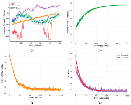
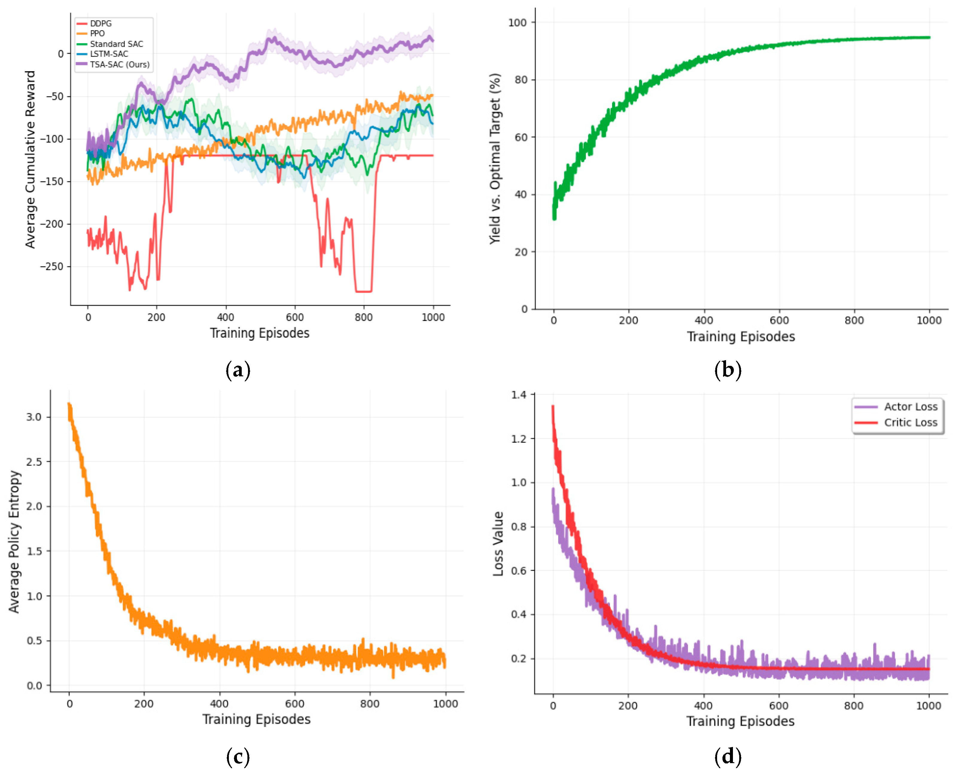
The learning efficiency, stability, and final convergence level were analyzed to evaluate DRL algorithms’ performance (Figure 5). In Figure 5a, all DRL algorithms start from a negative reward because of the inherent defect of an untrained random strategy in an environment with costs and penalties. TSA-SAC (ours) surpasses all other algorithms at approximately 300 rounds and first becomes positive with a stable training process. The final average cumulative return of our approach is significantly higher than all the comparison algorithms with the highest asymptotic performance.

Figure 5. Analysis of the DRL agents’ training dynamics and the internal learning process of the proposed TSA-SAC agent, including (a) a comparative plot of the average cumulative reward for all DRL agents over 1000 training episodes, in which the solid lines represent the average values of multiple independent experiments, and the shaded areas represent the standard deviations; (b) the yield performance evolution of the TSA-SAC agent; (c) the average policy entropy evolution for the TSA-SAC agent; (d) the convergence of the Actor and Critic loss functions for the TSA-SAC agent.

Figure 5b presents the learning progress of TSA-SAC in terms of output. The curve exhibits a classic S-shaped growth pattern. It increases rapidly in the middle of the training process and gradually approaches an optimal target level of over 95% in the later stages. This indicates that the goal of maximizing cumulative rewards can effectively guide the model to achieve high production. Figure 5c reveals the “exploration–exploitation” behavior of TSA-SAC during the training process. The entropy of the policy rapidly decreases from a relatively high initial value and stabilizes at a relatively small positive value after approximately 400 rounds. This suggests that after sufficient exploration, the policy becomes stable, but always maintains a slight randomness to adapt to environmental changes. Figure 5d shows that the loss functions of the Actor and Critic both rapidly decrease from a high level and eventually converge to a lower, stable fluctuating range.

The reward values were compared during the operation of each reinforcement learning algorithm under the same environmental conditions, including the convergence speed, asymptotic performance, and training stability. After completing the performance evaluation of the algorithms, we combined all the trained optimal policy models with traditional methods to conduct the final performance evaluation on an independent test year. The evaluation was carried out based on the multidimensional indicator system we established (Table 5). Compared with FE, TSA-SAC achieved an 8.4% increase in output while saving 22.1% of irrigation water. TSA-SAC was able to significantly reduce the cumulative stress days (CWSD) from the standard SAC’s 8.1 days to 2.3 days. This validates the effectiveness of our dynamic penalty function in heavily penalizing the stress term. In terms of irrigation water use efficiency (IWUE) indicators, TSA-SAC reached a level of 19.6 kg/ha/mm, overcoming all other benchmark methods.

Table 5. Comprehensive performance comparison of different irrigation strategies under climate test years (2022–2024).

Strategy	Yield (kg/ha)	Irrigation (mm)	IWUE (kg/ha/mm)	CWSD (Days)
FE	$6845\pm 156$	485 ± 23	14.1 ± 0.8	25.3 ± 4.1
DDPG	$7156\pm 198$	428 ± 31	16.7 ± 1.2	9.8 ± 2.8
PPO	$7089\pm 167$	435 ± 28	16.3 ± 1.1	10.5 ± 3.0
SAC	7203 ± 143	418 ± 22	17.2 ± 0.8	8.1 ± 2.1
LSTM-SAC	7298 ± 128	395 ± 18	18.5 ± 0.9	4.2 ± 1.5
TSA-SAC (Ours)	7421 ± 112	378 ± 16	19.6 ± 0.8	2.3 ± 0.9

Note: The values represent the mean ± standard deviation of 10 independent repeated experiments. Independent two-sample t-tests confirm statistically significant improvements of TSA-SAC over the FE strategy for yield, irrigation, and IWUE (p < 0.05). CWSD refers to the number of days when the water stress factor SWFAC is greater than 0.5.

We introduced 10% Gaussian noise to the observation variables during the inference phase. Under these noisy conditions, the agent maintained a high performance level, with the average yield remaining at 7315 ± 150 kg/ha (a decrease of only 1.4%) and IWUE at 19.1 kg/ha/mm. This confirms that the learned policy captures robust environmental features rather than overfitting to precise noise-free simulation states.

3.2. Analysis of the Ablation Experiment Results

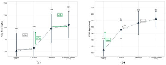
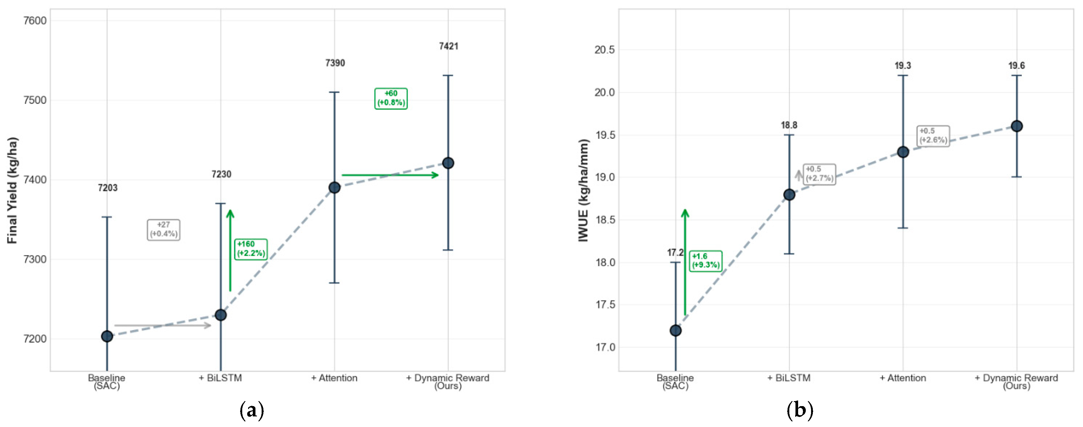
In the ablation study, improvement modules were successively added to the standard SAC (Baseline), including temporal modeling (+BiLSTM), dual-attention mechanism (+Attention), and dynamic reward function (+Dynamic Reward). All models were trained and evaluated under the same conditions, and the performance evolution of all models was analyzed using final yield and IWUE (Figure 6).

Figure 6. Results of the ablation study of the TSA-SAC agent, which illustrates the incremental performance improvement on (a) final yield and (b) irrigation water use efficiency (IWUE).

Adding BiLSTM, the final yield increased 27 kg/ha (+0.4%), and the IWUE increased from 17.2 to 18.8 kg/ha/mm (+9.3%). Independent t-tests (N = 10) confirmed that this improvement in IWUE is statistically significant (p < 0.05), demonstrating that temporal modeling can significantly reduce ineffective and redundant irrigation. Then, adding the dual-attention mechanism (+Attention), the final yield increased 160 kg/ha (+2.2%), and the IWUE increased 0.5 kg/ha/mm (+2.7%). This yield increase showed a significant improvement trend over the baseline (p < 0.05). It indicates the model can better avoid yield losses caused by stress by focusing on water stress during the water demand peak. At last, adding the dynamic reward function (+Dynamic Reward), the yield reached the highest value of 7421 kg/ha (+0.8%), and IWUE also reached the peak value of 19.6 kg/ha/mm (+2.6%).

3.3. Model Interpretability Analysis

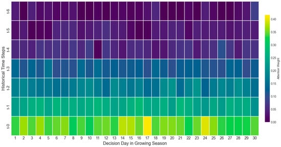
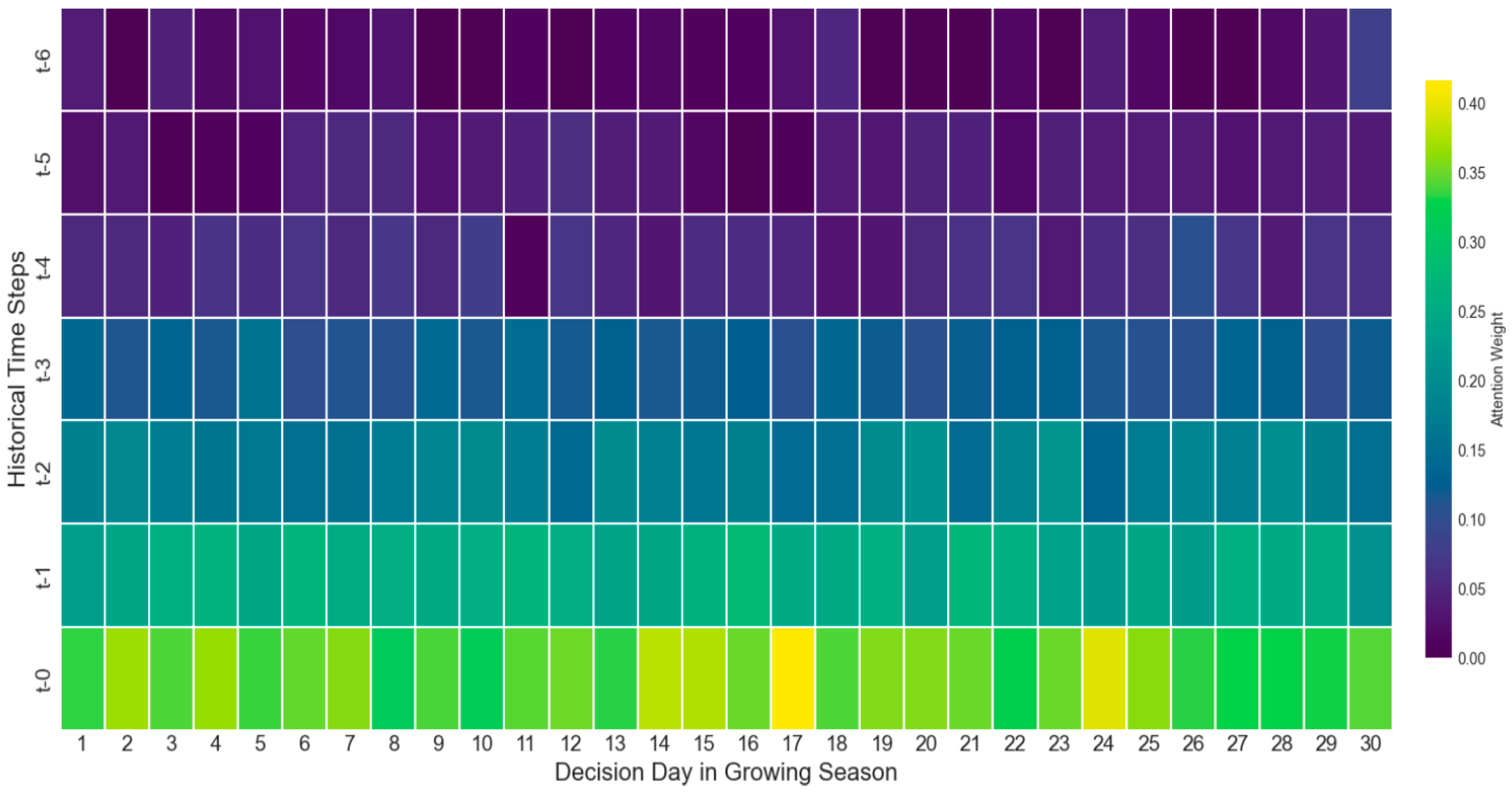
Although deep reinforcement learning models have demonstrated remarkable performance in complex decision-making tasks, their “black box” nature often limits their practical application and trustworthiness in critical fields. A visual analysis of TSA-SAC’s internal attention mechanism and decision-making behavior was conducted over a complete growing season. Figure 7 shows the distribution of the agent’s time attention weights during daily decisions within 30 days. The model’s attention weights always concentrated on the most recent 0–2 days (t-0 to t-2). On the 17th and 24th days, the model’s attention to the current state (t-0) reached a peak due to sudden rainfall and strong winds. This confirms the model can immediately identify and respond to this high-information input.

Figure 7. Heatmap of the temporal attention weights, in which the x-axis represents the growing days, and the y-axis represents the historical time steps (t-0 is the current day, t-6 is six days ago).

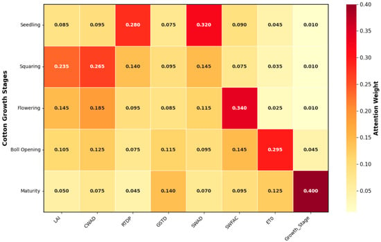
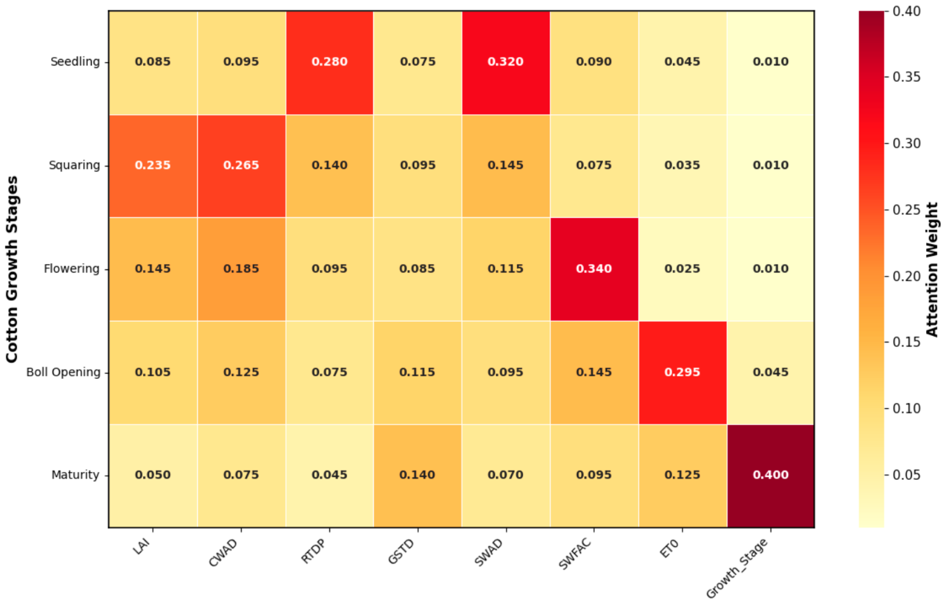
A heatmap was developed to present the average attention weight distribution of the model for 8 different state characteristics during the five key growth periods of cotton (Figure 8). The model prioritizes the feature with a higher attention during a particular growth stage. When the seedlings emerge from the soil, RTDP (0.280) and SWAD (0.320) showed the highest attention weights. This highlights the model’s focus on initial root establishment and immediate soil water availability. During the squaring stage, attention notably shifted to LAI (0.235) and CWAD (0.265), suggesting the model monitors both plant structure and cumulative growth. For the flowering stage, SWFAC (0.340) received increased attention because of the high sensitivity to water stress, which directly impacts flower retention and yield. Similarly, the boll-opening stage, ET0 (0.295), received high attention. While SWFAC remains crucial for boll development, ET0’s increased weight suggests the model considers cumulative water demand and potential atmospheric deficits. The emerging importance of the GSTD may indicate a transition towards later-season management, potentially including deficit irrigation for boll opening. In the maturity stage, there is a distinct shift, with the highest attention weight explicitly placed on the Growth_Stage code (0.400). This indicates that at the season’s end, the model primarily relies on phenological timing, as water demands typically decrease, and controlled water deficits may be applied to facilitate defoliation and harvest. Concurrently, weights for LAI, CWAD, and SWAD significantly decreased, reflecting their reduced relevance for irrigation decisions in this final stage.

Figure 8. Heatmap of the average feature attention weights, in which the horizontal axis represents the input features, and the vertical axis represents the five critical cotton growth stages. The color intensity and numerical values within each cell indicate the average attention weight, and darker reddish colors mean higher attention.

In practice, the agent outputs the executable irrigation amount, while the attention weights serve as a visual tool for human operators to validate the decision logic.

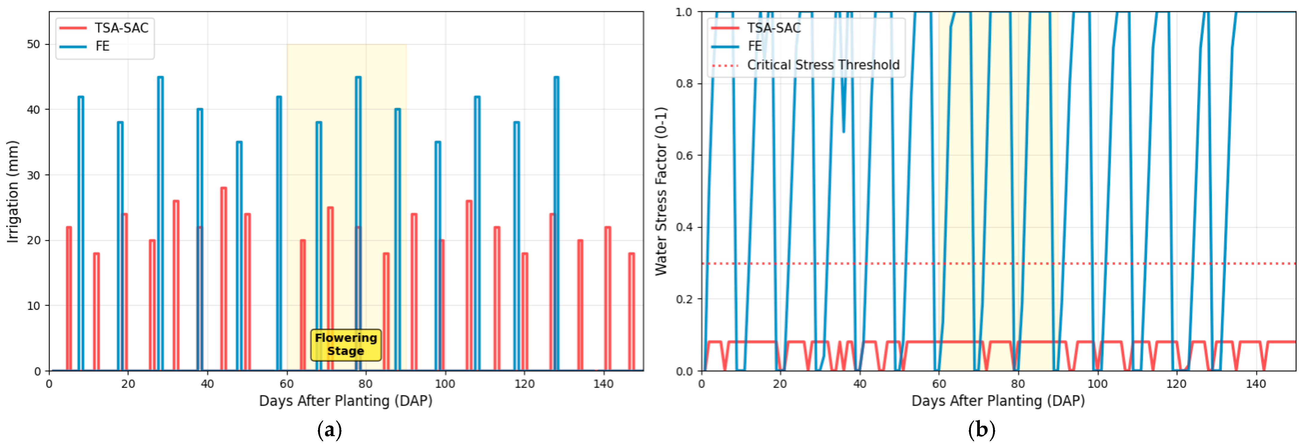
The comparison of the daily decision-making trajectories was conducted between TSA-SAC and FE (Figure 9). TSA-SAC applies irrigation in small and frequent increments using a proactive and precise water replenishment approach. FE tends to apply larger irrigation volumes over short intervals. The yellow-shaded flowering stage highlights a period of high water demand, where TSA-SAC maintains its refined irrigation pattern, avoiding over-irrigation while ensuring adequate water supply (Figure 9a). A red dashed line marks the critical stress threshold in Figure 9b. Results show TSA-SAC consistently maintains the water stress factor at very low, near-zero levels throughout the entire growing season, below the critical threshold. This indicates TSA-SAC prevents crops from experiencing detrimental water stress. In contrast, the FE strategy often causes the water stress factor to exceed the critical threshold, especially in mid-to-late growth stages, exposing crops to periodic and severe water stress that maybe negatively impact yield and quality.

Figure 9. Comparison of irrigation schedules and resulting crop stress for TSA-SAC versus the farmer experience (FE) baseline, including (a) daily irrigation decisions (mm) and (b) daily water stress factor (SWFAC, 0–1), where 0 means no stress and 1 means maximum stress. Red bars represent TSA-SAC’s decisions, and blue bars illustrate the FE strategy.

TSA-SAC’s decision adopts the principle of a few times with small amounts, and can carry out preventive water replenishment before the arrival of the critical flowering stage (Figure 9a). This is also reflected in the water stress factor comparison (Figure 9b). The FE strategy led to periodic and frequent severe stress exceeding the critical stress threshold. In contrast, the TSA-SAC strategy kept the water stress factors throughout the growing season at low and safe levels.

4. Discussion

4.1. Performance Superiority

This study proposed and verified an integrated intelligent irrigation decision-making framework (TSA-SAC) that combines the DSSAT crop model with an improved reinforcement learning method. The experimental results clearly demonstrated that this framework can outperform standard DRL algorithms in increasing both cotton yield and water use efficiency. Specifically, as shown in Table 5, TSA-SAC achieved a cotton yield of 7421 kg/ha, which is an 8.4% increase over the FE strategy. It also saved 22.1% of irrigation water and boosted irrigation water use efficiency (IWUE) to 19.6 kg/ha/mm, surpassing all benchmark algorithms.

It is usually hard to solve optimization methods in the complex and nonlinear dynamic environment constructed by DSSAT. Our method, TSA-SAC, successfully explored and converged to an approximately optimal long-term strategy in this high-dimensional state-action space through its trial-and-error learning and value function approximation capabilities. Interpretability analysis further proves that TSA-SAC has learned not just a set of scattered rules, but a kind of wisdom of dynamic trade-offs. For instance, as shown in Figure 8, the model dynamically adjusts its focus on key input features based on cotton’s physiological needs at different growth stages. It learns to perform preventive water replenishment before critical periods like flowering, which are highly sensitive to water stress. The model’s rapid convergence and stability during training are also advantages. As Figure 5a illustrates, TSA-SAC surpassed all other algorithms after approximately 300 training episodes. This indicates its improved algorithm design allows for efficient learning in complex agricultural environments, accelerating strategy acquisition. Ablation experiments (Figure 6) further validated the effectiveness of each innovative module. Temporal modeling (BiLSTM) reduced ineffective irrigation, the dual-attention mechanism effectively avoided yield losses from stress during peak demand, and the dynamic reward function further optimized yield and IWUE.

4.2. Generalizability and Adaptability

In this work, the proposed TSA-SAC framework integrates a BiLSTM module and an attention mechanism that captures temporal meteorological patterns to handle extreme weather and soil variability. The DRL agent makes decisions based on state feedback and inherently adapts to changes in soil hydraulic properties. The dynamic reward function serves as a generic template. We believe this framework is able to be adapted to some other crops by aligning the penalty weights with their critical growth stages. The balance between yield and water conservation can be tuned by adjusting the weight ratio to meet different regional goals. The framework architecture is transferable, but retraining is necessary for different crops to align the policy with their specific biological characteristics and reward weights. In addition, energy and economic costs can be integrated as negative terms in the reward function to prevent excessively frequent irrigation. Similarly, soil salt content can be included in the state space with penalties for high salinity levels.

4.3. Limitations and Pathway to Field Deployment

In this work, the years 2022–2024 were used to calibrate the crop parameters; they also served as the test set for the DRL agent. However, the agent was trained exclusively on historical data (2014–2020) and had no prior knowledge of the 2022–2024 weather sequences. This setup tests the agent’s ability to generalize to new meteorological conditions. Furthermore, since all comparison strategies (TSA-SAC, FE, and PPO) were evaluated in the environment, the relative performance improvements remain a robust indicator of algorithmic superiority. In practical application, agronomic expertise is necessary to collect local data to calibrate the DSSAT model. We distinguish between cloud-based training and on-site deployment regarding cost. Training the agent requires high-performance GPUs and significant computing resources, and the trained policy network is simply a lightweight file. It can be embedded into low-cost agricultural controllers or edge devices for real-time inference [51]. A Digital twin-based online learning framework can also be used as an option. This method uses real-time sensor data to synchronize the local DSSAT model, allowing the agent to safely adapt to seasonal trends. Additionally, a rule-based safety layer will be integrated to constrain irrigation actions within safe agronomic limits to ensure operational stability.

5. Conclusions

This study established an intelligent irrigation decision-making method (TSA-SAC) integrating a crop model with deep reinforcement learning. The BiLSTM-Attention mechanism helped to capture long-term environmental dependencies in agricultural POMDPs. The proposed dynamic reward function successfully embedded agronomic domain knowledge into the AI’s learning process, and enabled the agent to autonomously balance the trade-off between yield maximization and water conservation. Future work will focus on developing a ‘Digital Twin’ framework that calibrates the DSSAT model daily using IoT sensor data, allowing the agent to fine-tune its policy in real-time to match current seasonal trends.

References

- Kay, M.; Bunning, S.; Burke, J.; Boerger, V.; Bojic, D.; Bosc, P.M.; Ziadat, F. The State of the World’s Land and Water Resources for Food and Agriculture 2021: Systems at Breaking Point; FAO: Rome, Italy, 2022. [Google Scholar]
- Pastor, A.V.; Palazzo, A.; Havlik, P.; Biemans, H.; Wada, Y.; Obersteiner, M.; Ludwig, F. The global nexus of food–trade–water sustaining environmental flows by 2050. Nat. Sustain. 2019, 2, 499–507. [Google Scholar] [CrossRef] [Scilit]
- Harika, K.; Halesha, P.; Singh, A.K.; Agnihotri, P.; Rajpoot, S.K.; Prasad, S.K.; Bhushan, C. Smart Weather-Based Irrigation Scheduling Technologies. In Modern Technology for Sustainable Agriculture; Springer Nature: Cham, Switzerland, 2025; pp. 129–147. [Google Scholar]
- Pramanik, M.; Khanna, M.; Singh, M.; Singh, D.K.; Sudhishri, S.; Bhatia, A.; Ranjan, R. Automation of soil moisture sensor-based basin irrigation system. Smart Agric. Technol. 2022, 2, 100032. [Google Scholar] [CrossRef] [Scilit]
- Palumbo, M.; D’Imperio, M.; Tucci, V.; Cefola, M.; Pace, B.; Santamaria, P.; Montesano, F.F. Sensor-based irrigation reduces water consumption without compromising yield and postharvest quality of soilless green bean. Agronomy 2021, 11, 2485. [Google Scholar] [CrossRef] [Scilit]
- Bonelli, L.; Montesano, F.F.; D’Imperio, M.; Gonnella, M.; Boari, A.; Leoni, B.; Serio, F. Sensor-based fertigation management enhances resource utilization and crop performance in soilless strawberry cultivation. Agronomy 2024, 14, 465. [Google Scholar] [CrossRef] [Scilit]
- El-Naggar, A.G.; Hedley, C.B.; Horne, D.; Roudier, P.; Clothier, B.E. Soil sensing technology improves application of irrigation water. Agric. Water Manag. 2020, 228, 105901. [Google Scholar] [CrossRef] [Scilit]
- Sharma, K.; Irmak, S.; Kukal, M.S. Propagation of soil moisture sensing uncertainty into estimation of total soil water, evapotranspiration and irrigation decision-making. Agric. Water Manag. 2021, 243, 106454. [Google Scholar] [CrossRef] [Scilit]
- Vellidis, G.; Liakos, V.; Andreis, J.H.; Perry, C.D.; Porter, W.M.; Barnes, E.M.; Migliaccio, K.W. Development and assessment of a smartphone application for irrigation scheduling in cotton. Comput. Electron. Agric. 2016, 127, 249–259. [Google Scholar] [CrossRef] [Scilit]
- Han, C.; Yang, H.; Payyala, D.; Xia, T.; Liu, J.; Zhang, Y.; Chen, Y. CornSoyWater, a web application for irrigation decision support on corn and soybean. Agric. Water Manag. 2025, 313, 109454. [Google Scholar] [CrossRef] [Scilit]
- Feng, X.; Bi, S.; Li, H.; Qi, Y.; Chen, S.; Shao, L. Soil moisture forecasting for precision irrigation management using real-time electricity consumption records. Agric. Water Manag. 2024, 291, 108656. [Google Scholar] [CrossRef] [Scilit]
- Rasheed, M.W.; Tang, J.; Sarwar, A.; Shah, S.; Saddique, N.; Khan, M.U.; Sultan, M. Soil moisture measuring techniques and factors affecting the moisture dynamics: A comprehensive review. Sustainability 2022, 14, 11538. [Google Scholar] [CrossRef] [Scilit]
- Melo, M.L.A.D. Process-Based Modeling of Root Water Uptake and Plant Available Water at the Field Scale. Ph.D. Thesis, University of São Paulo, São Paulo, Brazil, 2024. [Google Scholar]
- Jones, J.W.; Tsuji, G.Y.; Hoogenboom, G.; Hunt, L.A.; Thornton, P.K.; Wilkens, P.W.; Singh, U. Decision support system for agrotechnology transfer: DSSAT v3. In Understanding Options for Agricultural Production; Springer: Dordrecht, The Netherlands, 1998; pp. 157–177. [Google Scholar]
- Keating, B.A.; Carberry, P.S.; Hammer, G.L.; Probert, M.E.; Robertson, M.J.; Holzworth, D.; Smith, C.J. An overview of APSIM, a model designed for farming systems simulation. Eur. J. Agron. 2003, 18, 267–288. [Google Scholar] [CrossRef] [Scilit]
- Gavasso-Rita, Y.L.; Papalexiou, S.M.; Li, Y.; Elshorbagy, A.; Li, Z.; Schuster-Wallace, C. Crop models and their use in assessing crop production and food security: A review. Food Energy Secur. 2024, 13, e503. [Google Scholar] [CrossRef] [Scilit]
- Zhao, Y.; Li, G.; Li, S.; Luo, Y.; Bai, Y. A review on the optimization of irrigation schedules for farmlands based on a simulation–optimization model. Water 2024, 16, 2545. [Google Scholar] [CrossRef] [Scilit]
- Danach, K.; Harb, H.; Hejase, H.J.; Saker, L. A Hybrid Metaheuristic Framework with Reinforcement Learning-Based Heuristic Selection for Large-Scale Combinatorial Optimization. Eur. J. Pure Appl. Math. 2025, 18, 6602. [Google Scholar] [CrossRef] [Scilit]
- Lyu, J.; Jiang, Y.; Xu, C.; Liu, Y.; Su, Z.; Liu, J.; He, J. Multi-objective winter wheat irrigation strategies optimization based on coupling AquaCrop-OSPy and NSGA-III: A case study in Yangling, China. Sci. Total Environ. 2022, 843, 157104. [Google Scholar] [CrossRef] [Scilit] [PubMed]
- Drogkoula, M.; Kokkinos, K.; Samaras, N. A comprehensive survey of machine learning methodologies with emphasis in water resources management. Appl. Sci. 2023, 13, 12147. [Google Scholar] [CrossRef] [Scilit]
- Fan, J.; Zheng, J.; Wu, L.; Zhang, F. Estimation of daily maize transpiration using support vector machines, extreme gradient boosting, artificial and deep neural networks models. Agric. Water Manag. 2021, 245, 106547. [Google Scholar] [CrossRef] [Scilit]
- Saggi, M.K.; Jain, S. A Survey Towards Decision Support System on Smart Irrigation Scheduling Using Machine Learning approaches. Arch. Comput. Methods Eng. 2022, 29, 4455–4478. [Google Scholar] [CrossRef] [Scilit]
- Goap, A.; Sharma, D.; Shukla, A.K.; Krishna, C.R. An IoT based smart irrigation management system using Machine learning and open source technologies. Comput. Electron. Agric. 2018, 155, 41–49. [Google Scholar] [CrossRef] [Scilit]
- Lindemann, B.; Müller, T.; Vietz, H.; Jazdi, N.; Weyrich, M. A survey on long short-term memory networks for time series prediction. Procedia CIRP 2021, 99, 650–655. [Google Scholar] [CrossRef] [Scilit]
- Yunita, A.; Pratama, M.I.; Almuzakki, M.Z.; Ramadhan, H.; Akhir, E.A.P.; Mansur, A.B.F.; Basori, A.H. Performance analysis of neural network architectures for time series forecasting: A comparative study of RNN, LSTM, GRU, and hybrid models. MethodsX 2025, 15, 103462. [Google Scholar] [CrossRef] [Scilit]
- Fathi, M.; Shah-Hosseini, R.; Moghimi, A. 3D-ResNet-BiLSTM model: A deep learning model for county-level soybean yield prediction with time-series Sentinel-1, Sentinel-2 imagery, and Daymet data. Remote Sens. 2023, 15, 5551. [Google Scholar] [CrossRef] [Scilit]
- Abioye, E.A.; Abidin, M.S.Z.; Mahmud, M.S.A.; Buyamin, S.; Ishak, M.H.I.; Abd Rahman, M.K.I.; Ramli, M.S.A. A review on monitoring and advanced control strategies for precision irrigation. Comput. Electron. Agric. 2020, 173, 105441. [Google Scholar] [CrossRef] [Scilit]
- Pattanayak, S.K.; Bhoyar, M.; Adimulam, T. Deep reinforcement learning for complex decision-making tasks. Int. J. Innov. Res. Sci. Eng. Technol. 2024, 13, 18205–18220. [Google Scholar]
- Liu, J.; Chang, F.; Yang, J.; Jie, X.; Lu, C.; Wang, C.; Xie, L.; Ma, L.; Su, H. Deep Reinforcement Learning for irrigation optimization: Advantages, opportunities, and challenges. Agric. Water Manag. 2025, 322, 110030. [Google Scholar] [CrossRef] [Scilit]
- Li, S.E. Reinforcement Learning for Sequential Decision and Optimal Control; Springer: Singapore, 2023. [Google Scholar]
- Orr, J.; Dutta, A. Multi-agent deep reinforcement learning for multi-robot applications: A survey. Sensors 2023, 23, 3625. [Google Scholar] [CrossRef] [Scilit]
- Nian, R.; Liu, J.; Huang, B. A review on reinforcement learning: Introduction and applications in industrial process control. Comput. Chem. Eng. 2020, 139, 106886. [Google Scholar] [CrossRef] [Scilit]
- Dogru, O.; Xie, J.; Prakash, O.; Chiplunkar, R.; Soesanto, J.; Chen, H.; Huang, B. Reinforcement learning in process industries: Review and perspective. IEEE/CAA J. Autom. Sin. 2024, 11, 283–300. [Google Scholar] [CrossRef] [Scilit]
- Ajagekar, A.; Mattson, N.S.; You, F. Energy-efficient AI-based control of semi-closed greenhouses leveraging robust optimization in deep reinforcement learning. Adv. Appl. Energy 2023, 9, 100119. [Google Scholar] [CrossRef] [Scilit]
- Chen, M.; Cui, Y.; Wang, X.; Xie, H.; Liu, F.; Luo, T.; Luo, Y. A reinforcement learning approach to irrigation decision-making for rice using weather forecasts. Agric. Water Manag. 2021, 250, 106838. [Google Scholar] [CrossRef] [Scilit]
- Saikai, Y.; Peake, A.; Chenu, K. Deep reinforcement learning for irrigation scheduling using high-dimensional sensor feedback. PLoS Water 2023, 2, e0000169. [Google Scholar] [CrossRef] [Scilit]
- Alibabaei, K.; Gaspar, P.D.; Assuncao, E.; Alirezazadeh, S.; Lima, T.M. Irrigation optimization with a deep reinforcement learning model: Case study on a site in Portugal. Agric. Water Manag. 2022, 263, 107480. [Google Scholar] [CrossRef] [Scilit]
- Liu, J.; Yang, J.; Jie, X.; Chang, F.; Ma, L.; Su, H. Optimizing irrigation scheduling using Deep Reinforcement Learning and crop growth model. In Proceedings of the 2025 ASABE Annual International Meeting, Toronto, ON, Canada, 13–16 July 2025; American Society of Agricultural and Biological Engineers: St. Joseph, MI, USA, 2025; p. 1. [Google Scholar]
- de Queiroz Pereira, G.; Renaux, D.P.B.; Lazzaretti, A.E. Comparative Analysis of Reinforcement Learning and Rule-Based System Approaches for Irrigation in Horticulture. IEEE Access 2025, 13, 90418–90432. [Google Scholar] [CrossRef] [Scilit]
- Kelly, T.D.; Foster, T.; Schultz, D.M. Assessing the value of deep reinforcement learning for irrigation scheduling. Smart Agric. Technol. 2024, 7, 100403. [Google Scholar] [CrossRef] [Scilit]
- Lobell, D.B.; Gourdji, S.M. The influence of climate change on global crop productivity. Plant Physiol. 2012, 160, 1686–1697. [Google Scholar] [CrossRef] [Scilit] [PubMed]
- Gautron, R.; Padrón, E.J.; Preux, P.; Bigot, J.; Maillard, O.A.; Emukpere, D. gym-DSSAT: A crop model turned into a Reinforcement Learning environment. arXiv 2022, arXiv:2207.03270. [Google Scholar] [CrossRef] [Scilit]
- Turchetta, M.; Corinzia, L.; Sussex, S.; Burton, A.; Herrera, J.; Athanasiadis, I.; Krause, A. Learning long-term crop management strategies with CyclesGym. In Advances in Neural Information Processing Systems (NeurIPS); Curran Associates, Inc.: Red Hook, NY, USA, 2022; Volume 35, pp. 11396–11409. [Google Scholar]
- Allen, R.G.; Pereira, L.S.; Raes, D.; Smith, M. Crop Evapotranspiration—Guidelines for Computing Crop Water Requirements; FAO Irrigation and Drainage Paper 56; FAO: Rome, Italy, 1998; Volume 300, p. D05109. [Google Scholar]
- Haarnoja, T.; Zhou, A.; Abbeel, P.; Levine, S. Soft Actor-Critic: Off-Policy Maximum Entropy Deep Reinforcement Learning with a Stochastic Actor. In Proceedings of the 35th International Conference on Machine Learning (ICML), Stockholm, Sweden, 10–15 July 2018; PMLR: Stockholm, Sweden, 2018; Volume 80, pp. 1861–1870. [Google Scholar]
- Paulson, J.A.; Tsay, C. Bayesian optimization as a flexible and efficient design framework for sustainable process systems. Curr. Opin. Green Sustain. Chem. 2025, 51, 100983. [Google Scholar] [CrossRef] [Scilit]
- Yu, T.; Zhu, H. Hyper-Parameter Optimization: A Review of Algorithms and Applications. arXiv 2020, arXiv:2003.05689. [Google Scholar] [CrossRef] [Scilit]
- Raffin, A.; Hill, A.; Gleave, A.; Kanervisto, A.; Ernestus, M.; Dormann, N. Stable-Baselines3: Reliable Reinforcement Learning Implementations. J. Mach. Learn. Res. 2021, 22, 12348–12355. [Google Scholar]
- Lillicrap, T.P.; Hunt, J.J.; Pritzel, A.; Heess, N.; Erez, T.; Tassa, Y.; Silver, D.; Wierstra, D. Continuous control with deep reinforcement learning. In Proceedings of the 4th International Conference on Learning Representations (ICLR), San Juan, Puerto Rico, 2–4 May 2016. [Google Scholar]
- Schulman, J.; Wolski, F.; Dhariwal, P.; Radford, A.; Klimov, O. Proximal Policy Optimization Algorithms. arXiv 2017, arXiv:1707.06347. [Google Scholar] [CrossRef] [Scilit]
- Yang, J.; Liu, J.; Jie, X.; Chang, F.; Ma, L.; Su, H. Optimizing Irrigation Management Using Digital Twin and Image-based 3D Reconstruction of Plant. In Proceedings of the 2025 China Automation Congress (CAC), Harbin, China, 10–12 October 2025; IEEE: New York, NY, USA, 2025; pp. 1–6. [Google Scholar]
Disclaimer/Publisher’s Note: The statements, opinions and data contained in all publications are solely those of the individual author(s) and contributor(s) and not of MDPI and/or the editor(s). MDPI and/or the editor(s) disclaim responsibility for any injury to people or property resulting from any ideas, methods, instructions or products referred to in the content. |
© 2025 by the authors. Licensee MDPI, Basel, Switzerland. This article is an open access article distributed under the terms and conditions of the Creative Commons Attribution (CC BY) license (https://creativecommons.org/licenses/by/4.0/).