Article

Characterizing Growth and Estimating Yield in Winter Wheat Breeding Lines and Registered Varieties Using Multi-Temporal UAV Data

1
Xuzhou Institute of Agricultural Sciences in Jiangsu Xuhuai District, Xuzhou 221131, China
2
Agricultural College of Yangzhou University, Yangzhou University, Yangzhou 225009, China
*
Author to whom correspondence should be addressed.
These authors contributed equally to this work.
Agriculture 2025, 15(24), 2554; https://doi.org/10.3390/agriculture15242554
Submission received: 16 October 2025 / Revised: 3 December 2025 / Accepted: 8 December 2025 / Published: 10 December 2025

Abstract

Grain yield is one of the most critical indicators for evaluating the performance of wheat breeding. However, the assessment process, from early-stage breeding lines to officially registered varieties that have passed the DUS (Distinctness, Uniformity, and Stability) test, is often time-consuming and labor-intensive. Multispectral remote sensing based on unmanned aerial vehicles (UAVs) has demonstrated significant potential in crop phenotyping and yield estimation due to its high throughput, non-destructive nature, and ability to rapidly collect large-scale, multi-temporal data. In this study, multi-temporal UAV-based multispectral imagery, RGB images, and canopy height data were collected throughout the entire wheat growth stage (2023–2024) in Xuzhou, Jiangsu Province, China, to characterize the dynamic growth patterns of both breeding lines and registered cultivars. Vegetation indices (VIs), texture parameters (Tes), and a time-series crop height model (CHM), including the logistic-derived growth rate (GR) and the projected area (PA), were extracted to construct a comprehensive multi-source feature set. Four machine learning algorithms, namely a random forest (RF), support vector machine regression (SVR), extreme gradient boosting (XGBoost), and partial least squares regression (PLSR), were employed to model and estimate yield. The results demonstrated that spectral, texture, and canopy height features derived from multi-temporal UAV data effectively captured phenotypic differences among wheat types and contributed to yield estimation. Features obtained from later growth stages generally led to higher estimation accuracy. The integration of vegetation indices and texture features outperformed models using single-feature types. Furthermore, the integration of time-series features and feature selection further improved predictive accuracy, with XGBoost incorporating VIs, Tes, GR, and PA yielding the best performance (R2 = 0.714, RMSE = 0.516 t/ha, rRMSE = 5.96%). Overall, the proposed multi-source modeling framework offers a practical and efficient solution for yield estimation in early-stage wheat breeding and can support breeders and growers by enabling earlier, more accurate selection and management decisions in real-world production environments.

1. Introduction

One of the greatest challenges of the 21st century will be to improve crop production and crop quality to meet the growing demands for food from the growing population and increasing affluence. The most environmentally friendly way to meet these demands is through crop breeding programs to develop new crop varieties with improved traits [1,2]. The rationale of a breeding program is to select among a large number of varieties with superior phenotypes for better yield and quality, tolerance to biotic and abiotic stresses, and high efficiency in cultivation, harvesting and processing [3,4]. Field-based phenotyping can be promising for gathering information about the plant traits per plot, which is important for the identification and description of breeding lines and registered varieties in agricultural practices [5].
Wheat (Triticum aestivum L.) is one of the most extensively cultivated cereal crops globally and plays a critical role in ensuring food security [6,7]. As population growth and climate change continue to intensify, increasing wheat yield has become a primary objective in breeding research [8,9]. In contemporary breeding programs, phenotypic trait and yield evaluation of wheat genotypes, from early-stage breeding lines to officially registered varieties that have passed the Distinctness, Uniformity, and Stability (DUS) test, still depend largely on destructive sampling, labor-intensive practices, and repeated field measurements [10,11]. These traditional methods constrain the scalability, efficiency, and cost-effectiveness of selection processes, particularly in large breeding populations and multi-location trials [12].
To overcome these limitations, high-throughput phenotyping (HTP) technologies have advanced rapidly in recent years, offering an efficient means of acquiring large-scale, quantitative trait data [13,14]. Among available approaches, multispectral remote sensing using unmanned aerial vehicle (UAV) has gained particular attention due to its low cost, non-destructive operation, high efficiency, and ability to capture multi-temporal information across extensive field areas [15,16,17]. Vegetation indices (VIs) derived from multispectral images are widely used to monitor canopy greenness, biomass accumulation, and photosynthetic activity [18,19,20]. Meanwhile, texture parameters (Tes) extracted from RGB imagery, including contrast, entropy, homogeneity, variance, and correlation, quantify the spatial organization of canopy surfaces. These metrics characterize variation, structural complexity, and uniformity within the canopy, and they provide informative signals that are linked to agronomic traits such as tiller density, growth vigor, and lodging susceptibility [21,22,23]. Additionally, canopy height information reconstructed from three-dimensional point cloud data, typically represented as crop height model (CHM), provides valuable structural indicators of crop development [24,25].
While numerous studies have demonstrated the value of UAV-derived features for monitoring crop growth and estimating biomass, the integration of multi-source and multi-temporal data for yield prediction remains limited, particularly for early-stage breeding lines and officially registered varieties [26,27]. Moreover, conventional static modeling approaches often overlook the explanatory power of growth dynamics in differentiating genotypes. Capturing phenotypic variation throughout the entire growing season continues to pose a significant challenge. Growth curve models offer a solution by quantifying temporal trajectories of phenotypic traits and enabling the extraction of physiological parameters such as growth rate and acceleration, which are closely linked to genotypic vigor and developmental timing [28,29,30]. To fully exploit the potential of high-dimensional phenotypic data, machine learning provides a flexible and powerful modeling framework that can capture non-linear relationships, accommodate high-dimensional inputs, and handle complex feature interactions, making it well-suited for yield estimation applications [31,32].
Machine learning has become an essential component of modern crop phenotyping because it enables the modeling of complex, nonlinear relationships between remotely sensed parameters and actual agronomic indicators. Unlike traditional linear regression methods, machine-learning algorithms can capture high-dimensional interactions among spectral, textural, and structural features, which are common in UAV-based phenotyping datasets. Recent studies demonstrate that machine-learning models, especially gradient boosting frameworks, can substantially outperform traditional approaches when integrating multi-temporal UAV features for yield prediction [33,34]. However, relatively few studies have systematically compared different machine-learning methods using multispectral, textural, and structural traits simultaneously, particularly in the context of early-generation breeding lines and officially registered varieties. This gap highlights the need for a comprehensive evaluation of machine-learning models under multi-source, multi-temporal phenotyping conditions.
This study aims to establish a multi-source and multi-temporal framework for phenotypic monitoring and yield estimation of wheat breeding lines and registered varieties. UAV-based multispectral imagery and canopy height data were collected across key wheat growth stages during the 2023–2024 growing season in Xuzhou, Jiangsu Province, China, to characterize full-season growth dynamics. Using these datasets, four machine learning algorithms were employed to model and estimate yield: Random Forest (RF), Support Vector Machine Regression (SVR), Extreme Gradient Boosting (XGBoost), and Partial Least Squares Regression (PLSR). The specific objectives of this study were (1) to characterize the growth dynamics of different types of wheat genotypes, including breeding lines and registered varieties in the Huang-Huai-Hai region; (2) to evaluate the contribution of different feature types and growth stages to yield prediction performance; and (3) to determine which UAV-based modeling strategies are most effective for supporting large-scale wheat breeding and variety evaluation.

2. Materials and Methods

2.1. Study Region Experimental Design

The field experiment was conducted during the 2023–2024 winter wheat growing season at the wheat breeding base of the Xuzhou Academy of Agricultural Sciences, located in Jiangsu Province, China (34°18′ N, 117°11′ E). The region has a warm temperate monsoon climate, with an average annual temperature of approximately 14.5 °C and an average annual precipitation of about 850 mm, making it well-suited for winter wheat cultivation. All wheat plots were planted on 10 October 2023, marking the beginning of the 2023–2024 growing season. Three experimental fields were established, designated as fields A, B, and C (Figure 1). Fields A and B were used for breeding trials and were planted with early-generation wheat lines under selection. Field C was used for variety trials and contained officially registered cultivars with granted plant variety rights, which were undergoing demonstration and regional adaptation testing. All fields followed a consistent plot design, with each plot measuring 7.5 m in length and 1.5 m in width, and a row spacing of 0.23 m, resulting in approximately 6 rows per plot. Throughout the growing season, irrigation was applied as needed based on crop growth and weather conditions to prevent drought stress. Weed, pest, and disease management was carried out in a timely manner according to field observations, using chemical or manual control methods recommended by local agronomic guidelines.

2.2. UAV Data Collection and Characterizing Growth and Estimating Yield Workflows

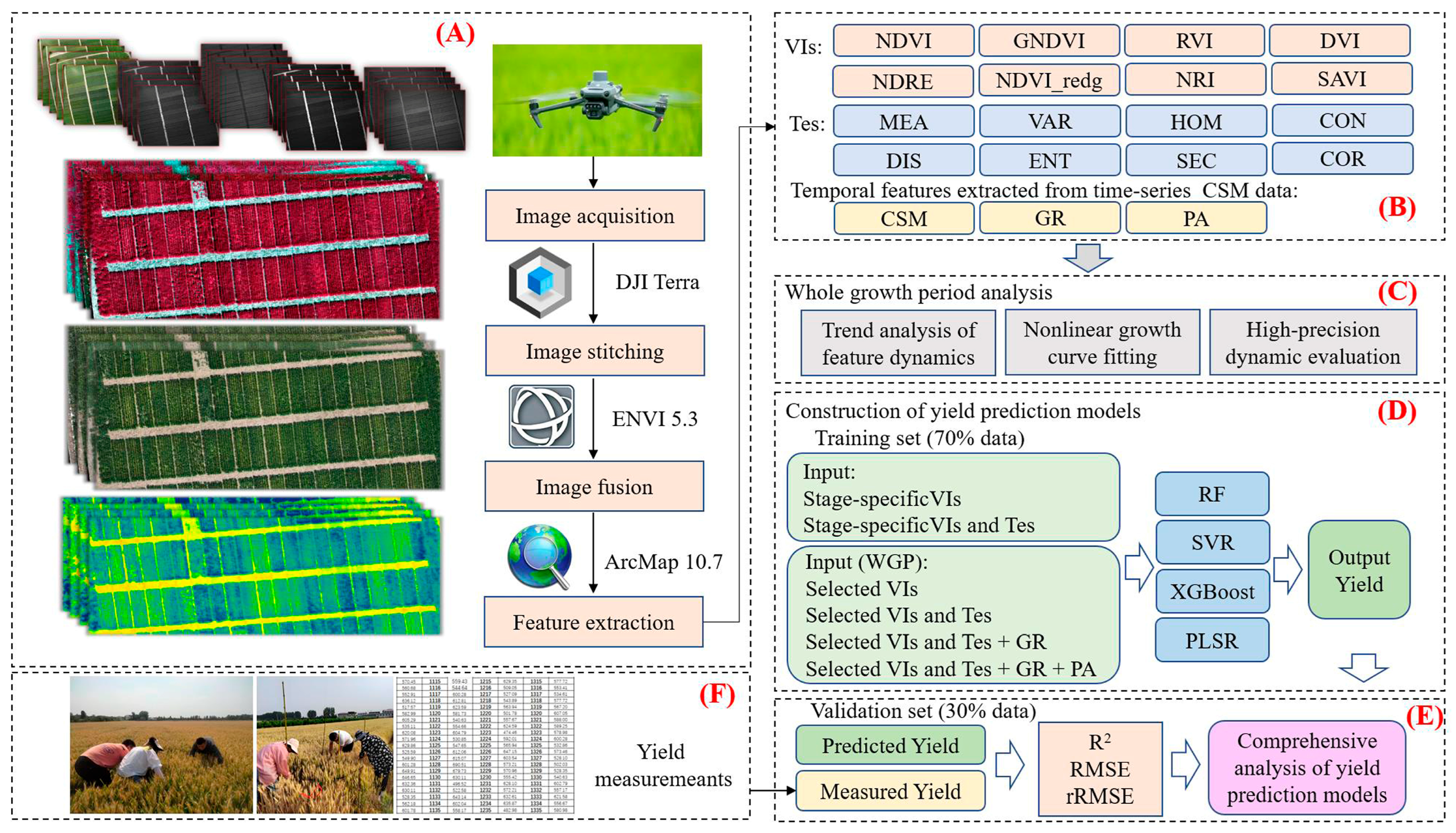
The overall technical workflow of this study is illustrated in Figure 2 and consists of four main stages: data collection, data processing, data analysis, and model development and validation. First, multi-temporal UAV-based remote sensing data of the wheat canopy were acquired, including multispectral imagery, RGB images, and canopy height data. These datasets were then preprocessed and used to extract multi-source phenotypic features, forming a comprehensive feature set. In the analysis stage, growth dynamics of both breeding lines and registered cultivars were characterized, and key temporal traits and physiological parameters were extracted. Finally, yield prediction models were developed based on the integrated multi-source and multi-temporal features, followed by model evaluation and comparative analysis of prediction accuracy. Finally, yield prediction models were developed using the integrated multi-source dataset, which included VIs, texture parameters, and canopy height derived temporal traits such as growth rate (GR) and projected area (PA). Model performance was then evaluated and compared across feature combinations to assess prediction accuracy.

2.3. Data Acquisition

2.3.1. UAV Data Collection and Preprocessing

UAV-based data acquisition was conducted at key growth stages of wheat using the DJI Mavic 3 Multispectral UAV platform equipped with RTK (SZ DJI Technology Co., Ltd., Shenzhen, China). Flights were carried out on 8 January 2024 (overwintering), 14 February 2024, 26 February 2024 (regreening), 19 March 2024 (jointing), 30 March 2024 (booting), 18 April 2024 (heading), 26 April 2024 (flowering), 2 May 2024, and 7 May 2024 (grain filling). The UAV platform is equipped with a multispectral camera containing four narrow-band sensors in the green (560 nm ± 16 nm), red (650 nm ± 16 nm), red-edge (730 nm ± 16 nm), and near-infrared (840 nm ± 26 nm) wavelengths, as well as an RGB visible light camera. It also supports structured light data acquisition for terrain modeling, enabling the generation of canopy height information. Before each flight, reflectance reference targets with 25%, 50%, and 75% calibrated reflectance were captured on the ground to obtain white-panel information. Images were taken at 20 m above ground level at the speed of 2 m/s, following the set path to cover each plot with the overlap of 85% to ensure high-quality image stitching and accurate three-dimensional reconstruction. All flights were conducted on clear, windless days between 10:00 and 14:00 to minimize shadow interference and ensure consistent lighting conditions across datasets.
The collected multispectral imagery was processed using DJI Terra 3.4.0 software (SZ DJI Technology Co., Ltd., Shenzhen, China) for image stitching, fusion, and radiometric correction, resulting in orthorectified reflectance maps within a unified coordinate system. RGB imagery was processed using Pix4Dmapper 4.5.6 software (Pix4DSA, Lausanne, Switzerland), to generate orthomosaic images and three-dimensional CHM. To enable accurate data extraction, we manually delineated vector boundaries for each plot in a GIS environment (ArcMap 10.7, ESRI, Redlands, CA, USA) according to the actual spatial layout of the breeding and variety trial fields. These vector regions, defined as regions of interest (ROI), were applied to batch-extract multi-temporal data from the multispectral images, RGB imagery, and canopy height layers [25]. The extracted data provided a consistent basis for multi-source phenotypic feature calculation and time-series analysis.

2.3.2. Measurement of Wheat Yield Data

At crop maturity, corresponding to the wax maturity to full maturity stage of wheat, each plot was manually harvested. Grain yield was measured after threshing and natural air-drying, and the final yield per plot was standardized to a moisture content of 13%, expressed as tons per hectare (t/ha). These measurements were used as ground-truth data for model training and validation. To ensure data quality, plots with missing plants, lodging, or mechanical errors were excluded. After quality control, 230 plots from Field 1, 398 plots from Field 2, and 272 plots from Field 3 were retained for subsequent analysis.

2.4. Extraction of Multi-Source Features

2.4.1. Spectral Features

Based on the radiometrically corrected multispectral images acquired by the multispectral platform, reflectance values from the original spectral bands were extracted. Eight VIs were then calculated using various band combinations (Table 1). These indices play a vital role in characterizing crop growth conditions, monitoring canopy dynamics, and identifying physiological traits. They are also considered key variables for predicting yield in other studies and crops [35,36,37].

2.4.2. Texture Features

Texture parameters were extracted from the orthomosaic RGB images using the gray-level co-occurrence matrix (GLCM) method. This method quantifies the spatial structural variation in an image by analyzing the grayscale relationships between adjacent pixels and is commonly used to characterize canopy uniformity, surface roughness, and structural complexity [38]. Texture calculations were performed in ENVI 5.3 software (Exelis Visual Information Solutions, Boulder, CO, USA) using the “Co-occurrence Measures” tool. A moving window size of 3 × 3 pixels was applied for GLCM computation, and eight texture parameters were extracted accordingly (Table 2). These features have demonstrated strong potential for describing canopy structural variation across different growth stages and have been shown to serve as effective supplementary variables for yield prediction [21,39,40].

2.4.3. Canopy Height Features

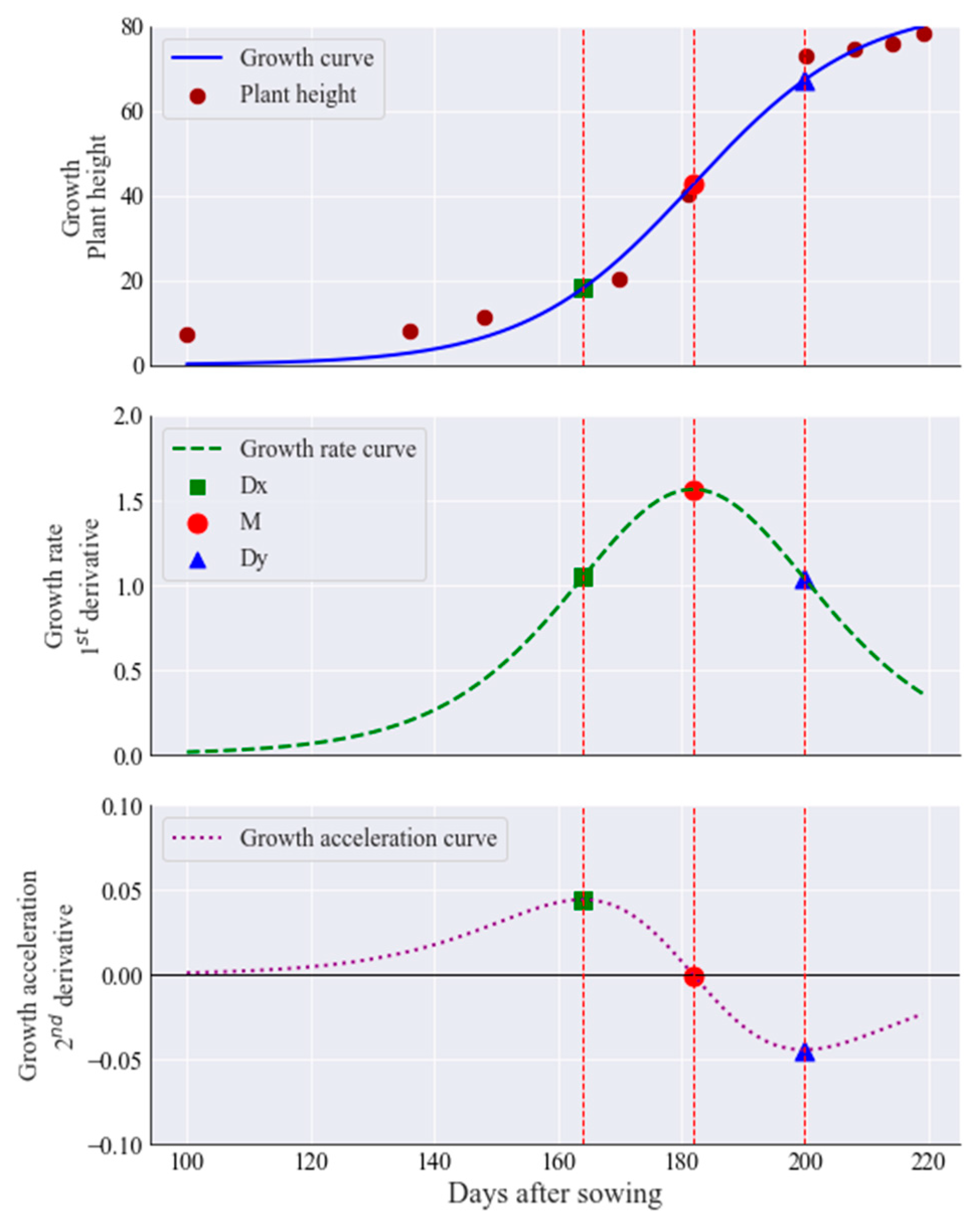
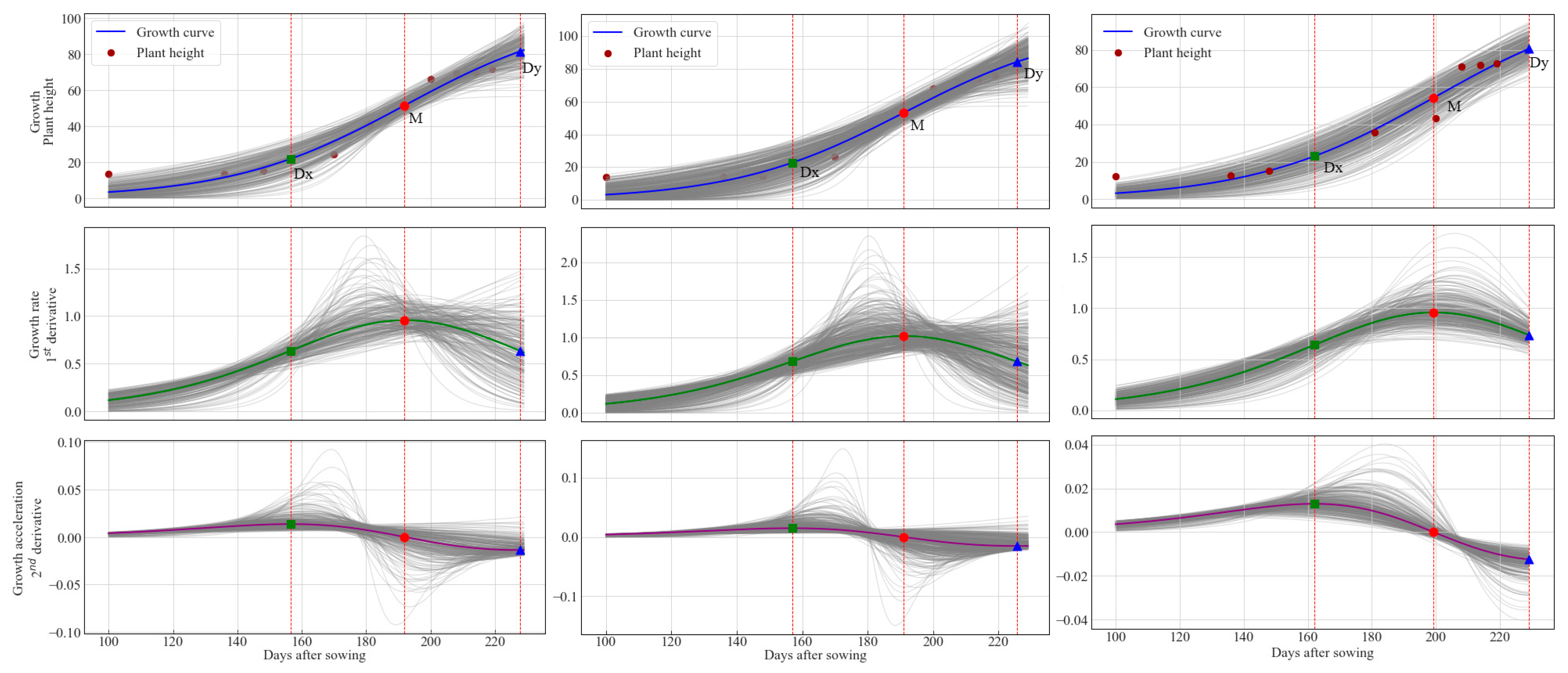
Canopy height for each plot was derived from the CHM generated using RGB imagery. Both the digital surface model (DSM) and digital terrain model (DTM) were produced through a Structure-from-Motion (SfM) workflow, including image matching, bundle adjustment, and dense point-cloud reconstruction. DSMs were generated for each growth stage, while the DTM was created using images acquired soon after sowing when the soil surface was exposed. Canopy height was then calculated as the difference between the DSM and DTM for each plot [41]. This features reflects the vertical growth status of the plants and serves as an important phenotypic indicator of crop vigor and canopy structure [42]. Canopy height was extracted at seven key growth stages and fitted using logistic growth curve (Equation (1)) to characterize the growth dynamics of different wheat genotypes. To further quantify growth dynamics, the first and second derivatives of the logistic curve with respect to DAS were calculated. The first derivative describes the instantaneous growth rate, and the second derivative describes the acceleration or deceleration of canopy height increase [43]. From these curves, three critical time points were extracted: Dx, corresponding to the time of maximum growth acceleration; Dy, corresponding to the time of minimum growth acceleration; and M, located between Dx and Dy, representing the time of maximum growth rate. An illustrative example of these critical points on a logistic growth curve is shown in Figure 3. The fitting of the logistic growth function as well as the computation of the first- and second-order derivatives in this study were performed in a Python 3.0 environment.
W(g) = Wf/[1 + exp − k(g − M)]
where W(g) is plant height at time g, Wf is the maximum value (upper asymptote), k is the relative growth rate in M, g denotes days after sowing (DAS), and M is the DAS at which the growth rate reaches its maximum (inflection point of the curve).

2.5. Yield Estimation Model Development

To effectively estimate wheat yield, this study employed four commonly used machine learning algorithms for regression modeling, including RF, SVR, XGBoost, and PLSR. RF is a non-parametric ensemble learning method based on decision trees, known for its strong ability to model nonlinear relationships and its robustness against overfitting [34]. SVR performs regression by constructing an optimal hyperplane and is well-suited for small-sample, high-dimensional datasets [44]. XGBoost is a gradient boosting framework that efficiently utilizes input features and demonstrates excellent generalization performance [45]. PLSR combines dimensionality reduction and regression, making it particularly suitable for datasets with severe multicollinearity among features [46].
Initially, yield estimation models were developed separately for each of the seven key wheat growth stages using VIs as the sole input features. Subsequently, the models were reconstructed by combining VIs with texture parameters to evaluate the predictive performance of the integrated feature sets at each stage. For whole growth period modeling, all spectral and texture features from multiple growth stages were aggregated independently. Feature selection was then performed using the feature importances_attribute, and the eight most informative VIs and texture features were retained from each category [47]. These selected features were further integrated with canopy height traits to form a multi-source dataset for model development. Finally, all four machine learning algorithms were trained using the integrated feature set, and their prediction accuracies were compared to evaluate the effectiveness of different modeling strategies.
For each modeling scenario, the dataset was randomly divided into a training set and a validation set, with two thirds of the samples used for model training and one third reserved for independent validation. Within the training set, hyperparameters of the four algorithms (RF, SVR, XGBoost, and PLSR) were tuned using grid search combined with ten-fold cross-validation. For RF, the number of trees and maximum tree depth were optimized. For SVR, the regularization parameter and kernel-related parameters were adjusted. For XGBoost, key hyperparameters such as the number of boosting rounds, learning rate, maximum tree depth, subsampling ratio, and column sampling ratio were calibrated. For PLSR, the optimal number of latent components was determined based on the minimum cross-validated prediction error. The final models were retrained on the full training set using the optimal hyperparameters and then evaluated on the validation set to compare the predictive accuracy of different feature combinations and algorithms. All model training, parameter tuning, and validation procedures were implemented in Python 3.0 using the scikit-learn machine-learning library.

2.6. Model Evaluation

To quantitatively assess the performance of different models in wheat yield estimation, two-thirds of the total samples were used for training and the remaining one-third for validation. Model accuracy was evaluated using three indicators, namely the coefficient of determination (R2), root mean square error (RMSE) and relative root mean square error (rRMSE) [48]. R2 quantifies the proportion of variance in the measured yield that is explained by the model, with values closer to 1 indicating a higher level of goodness of fit. RMSE measures the average deviation between predicted and measured yields, where lower values reflect higher accuracy. The rRMSE, defined as the ratio of RMSE to the mean measured yield, provides a normalized measure of error, facilitating comparison across models. R2, RMSE, and rRMSE were calculated using Equations (2), (3) and (4), respectively.
R 2 = 1 Σ i = 1 n y i y ^ i 2 Σ i = 1 n y i y ¯ 2
R M S E = Σ i = 1 n y i y ^ i 2 n
r R M S E = R M S E y ¯ × 100 %
where y i   and y ^ i   represent measured values and predicted values of yield, respectively; y is the average value of yield; and n is the number of samples.

3. Results

3.1. Distribution of Measured Yield Data

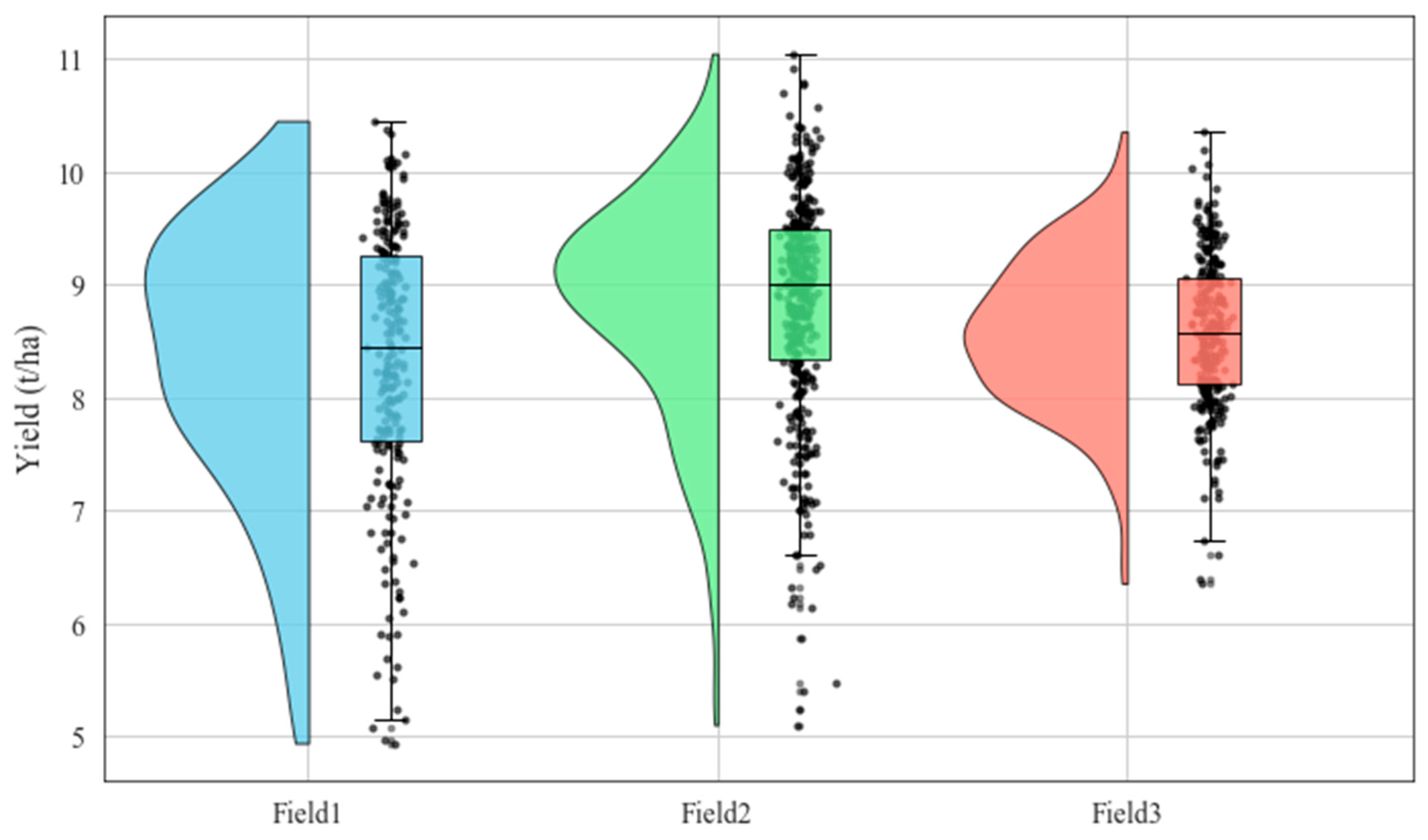
Figure 4 illustrates the yield distribution of wheat across the three fields. Overall, the mean yields among the fields were relatively close, but their distribution patterns and degrees of dispersion differed. Field 1 had a yield range of 5.0–10.5 t/ha, with a relatively concentrated distribution but slight skewness. Field 2 exhibited a wider yield range, reaching up to 11.0 t/ha, with a relatively smooth distribution and a median slightly higher than that of Field 1. Field 3 showed a more compact yield distribution, mainly concentrated between 8.0 and 9.0 t/ha, with fewer outliers and better overall stability. Fields 1 and 2 were planted with relatively immature early-generation breeding lines, whose genetic backgrounds were associated with larger yield differences and higher variability. In contrast, Field 3 was planted exclusively with officially registered varieties, which had a lower coefficient of variation and exhibited more stable performance.

3.2. Analysis of Spectral Features

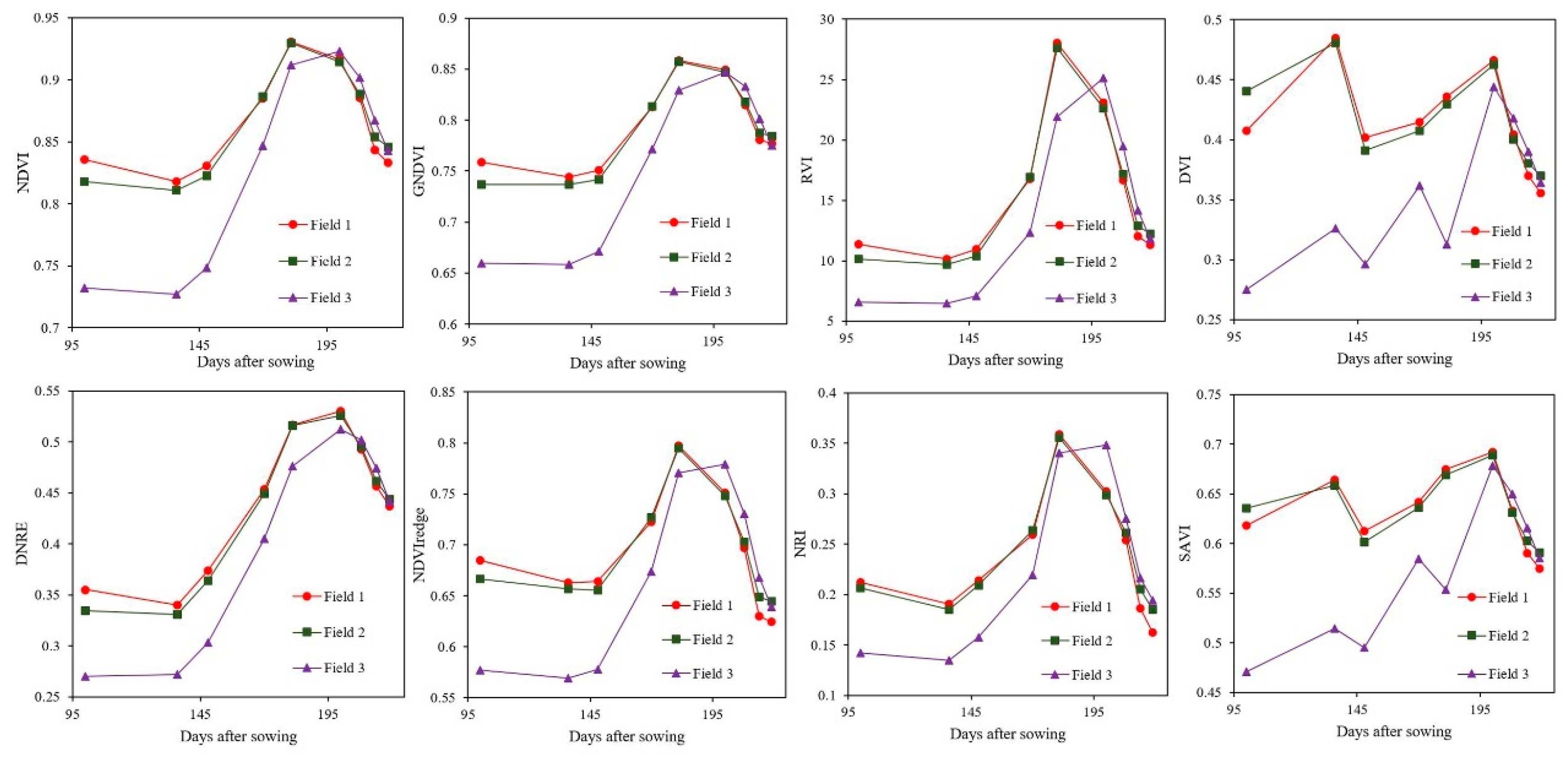
Figure 5 demonstrates the temporal dynamics of eight VIs across the three fields during the entire wheat growing season. For each field, VI values were calculated as the mean of all plots within the field at each flight date, ensuring a field-level representation of temporal trends. Overall, indices such as NDVI, GNDVI, DNRE, and NRI, which reflect canopy greenness and structural attributes, exhibited a high degree of consistency and synchrony among the fields. Between the overwintering and regreening stages, values reached a trough due to low temperatures that caused varying degrees of frost damage. From jointing to heading, all indices increased sharply and peaked around heading or the early flowering stage. This period corresponded to rapid canopy expansion, when both leaf area index and chlorophyll content typically reached their maximum, marking a critical stage for yield formation. As the crop entered the grain-filling and maturity stages, leaf senescence and chlorophyll degradation led to a marked decline in index values. Notably, Field 3 exhibited consistently lower VIs than Fields 1 and 2 during the early to mid-growth stages, suggesting delayed emergence or early growth suppression. However, in the later stages, the peak values of Field 3 approached those of the other fields, indicating a compensatory growth trend.

3.3. Analysis of Texture Features

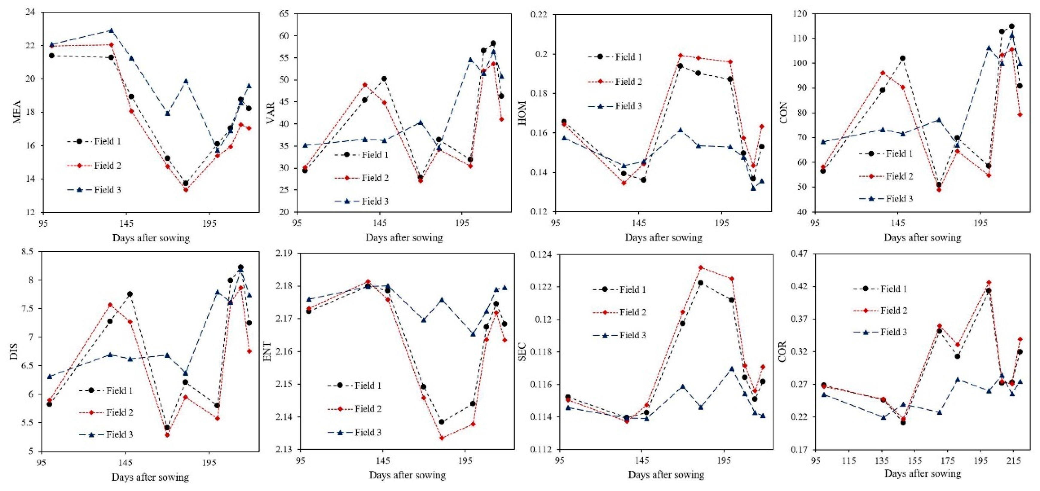
Throughout the entire wheat growing season, texture parameters exhibited clear temporal variation patterns, reflecting the dynamic evolution of canopy structure as growth progressed. As shown in Figure 6, during the early growth stage prior to jointing, plants gradually covered the soil surface, and variations in leaf arrangement and growth status resulted in pronounced changes in image gray levels. At this stage, indices such as MEA and ENT, which reflect texture irregularity, were relatively high. From jointing to flowering, plant height increased rapidly, leaves expanded more uniformly, and the canopy gradually closed, leading to a more stable structure and enhanced homogeneity. Correspondingly, indices such as HOM and SEC, which indicate structural stability, increased, while VAR, CON, and ENT declined. From heading to maturity, with spike emergence and leaf senescence, canopy structure shifted from a relatively uniform leaf-dominated surface to a mixed spike-leaf structure with increased vertical stratification, resulting in renewed heterogeneity and uneven texture patterns. In comparison across fields, Field 3 exhibited smaller fluctuations in texture parameters throughout the entire season, showing relatively smooth variation curves, which indicated more uniform growth status at each developmental stage.

3.4. Analysis of Canopy Height Features

In this study, the first- and second-order derivatives of the logistic curve were used to quantify differences in wheat growth dynamics. The first derivative describes the canopy growth rate, while the second derivative identifies acceleration changes, allowing key turning points in development to be captured. These derivative-based parameters provide an effective way to compare growth rhythm and developmental timing among different wheat types. Figure 7 shows the fitted logistic curves of canopy height and their first and second order derivatives for all plots across the three fields throughout the growing season. Each dashed line represents the fitted result of an individual plot, reflecting the variability of plant height growth within the population, while the bold solid line denotes the mean fitted curve of each field, capturing the overall canopy growth trend. By comparing the curve shapes and derivative characteristics across the three fields, clear differences can be observed in growth rhythm and population uniformity among the genotypes.
The canopy height dynamics of Field 1 and Field 2 were largely consistent. Both entered the rapid growth phase at approximately 150 days after sowing (DAS), with growth rate reaching its peak around 190 DAS, while the acceleration inflection point appeared during the same period. Growth acceleration then decreased and reached its minimum around 230 DAS. In contrast, Field 3 displayed distinct differences in canopy height features. The timing of maximum acceleration, the growth curve inflection point, and the minimum acceleration were all substantially delayed compared with Fields 1 and 2, indicating a postponed onset of stem elongation and canopy expansion. Moreover, the variance of growth acceleration in Field 3 was smaller, remaining within –0.04 to 0.04, suggesting a more synchronized growth rhythm among individual plants and a steadier, more balanced canopy expansion process. As officially registered and more mature variety, Field 3 demonstrated greater genetic stability and population coordination than the early generation breeding lines planted in Fields 1 and 2.

3.5. Optimal Machine Learning Model Selection for Yield Estimation

3.5.1. Stage-Specific Estimation Results

In the yield estimation models constructed at different growth stages, prediction accuracy generally improved as the crop developed. When only VIs were used as input variables (Table 3), all four models performed poorly before the booting stage, with validation R2 values generally below 0.3, RMSE above 0.9 t/ha, and rRMSE exceeding 10%. As the crop entered the flowering and grain filling stages, performance improved markedly. In particular, during the grain filling stage, all models achieved their highest R2 values, with the XGBoost model reaching 0.448 on the validation set and corresponding RMSE and rRMSE reduced to 0.717 t/ha and below 9%, respectively.
In comparison, the inclusion of texture parameters led to performance gains across all stages (Table 4), with the most pronounced improvements observed from heading to grain filling. For instance, in the grain filling stage, the RF model improved from an R2 of 0.452 to 0.508, while RMSE decreased to 0.711 t/ha and rRMSE further dropped to 8.25%. These results indicate that the integration of texture parameters with VIs enhanced the model’s ability to capture canopy spatial structure and density differences, thereby improving yield prediction. Overall, XGBoost and RF consistently delivered more stable and accurate predictions across stages, highlighting the advantage of ensemble learning methods in handling complex nonlinear relationships. Across the whole growth period, the grain filling stage remained the most representative for yield estimation.

3.5.2. Estimation Results for the Whole Growth Period

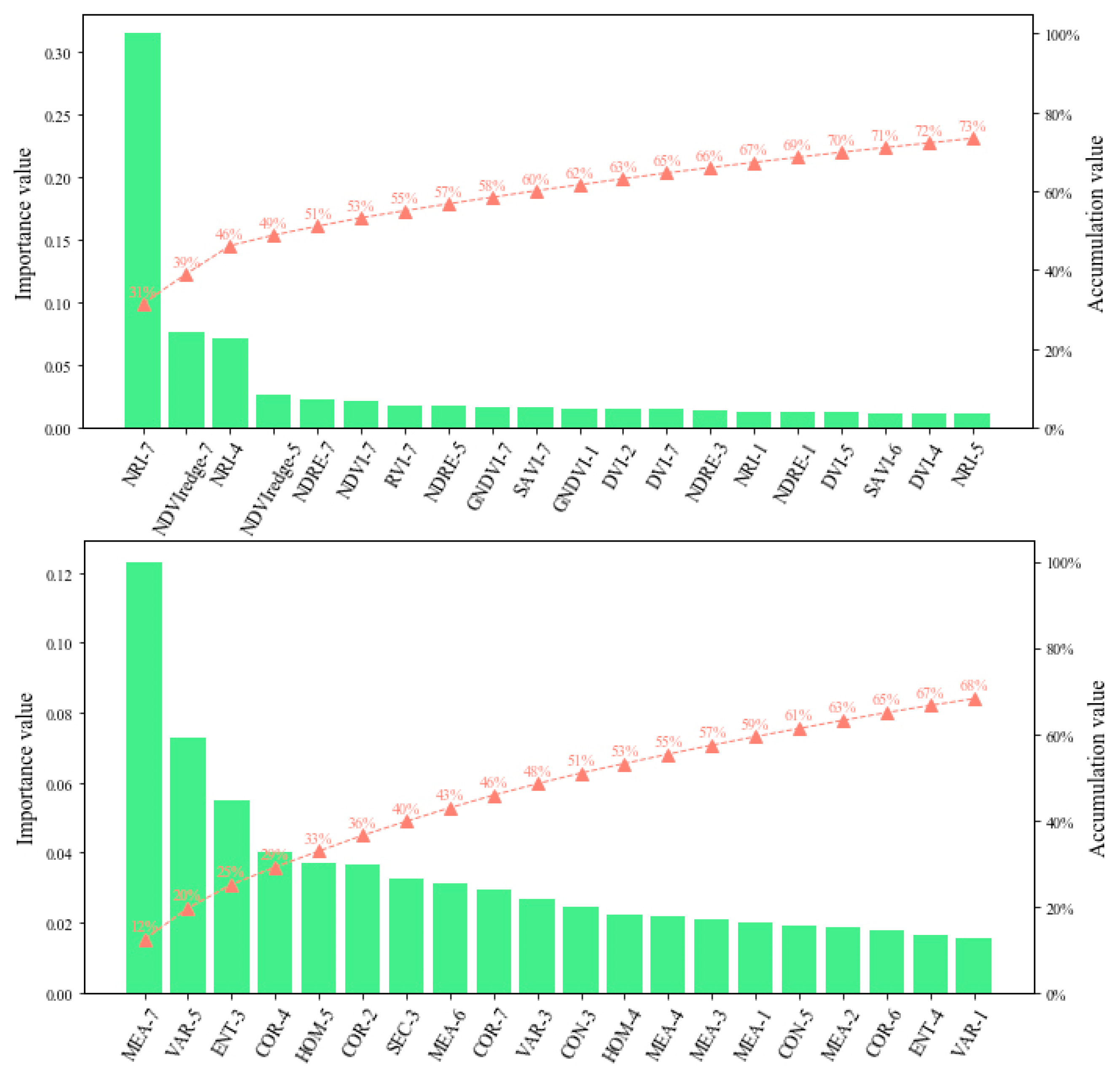
To identify the most informative phenotypic variables, feature selection was performed using the feature importance attribute, which quantifies the contribution of each input variable to prediction accuracy. Based on these importance scores, Figure 8 shows the importance ranking of spectral and texture parameters across the whole growth period based on feature importance analysis, with the top eight features selected as inputs for model development, respectively. In addition, GR and PA at whole growth period were derived from logistic growth curve fitting of canopy height and included as supplementary structural features. Four types of input feature combinations were constructed for yield estimation modeling: spectral features (VIs), spectral plus texture parameters (VIs + Tes), spectral plus texture parameters with growth rate (VIs + Tes + GR), and spectral plus texture parameters with growth rate and projected area (VIs + Tes + GR + PA).
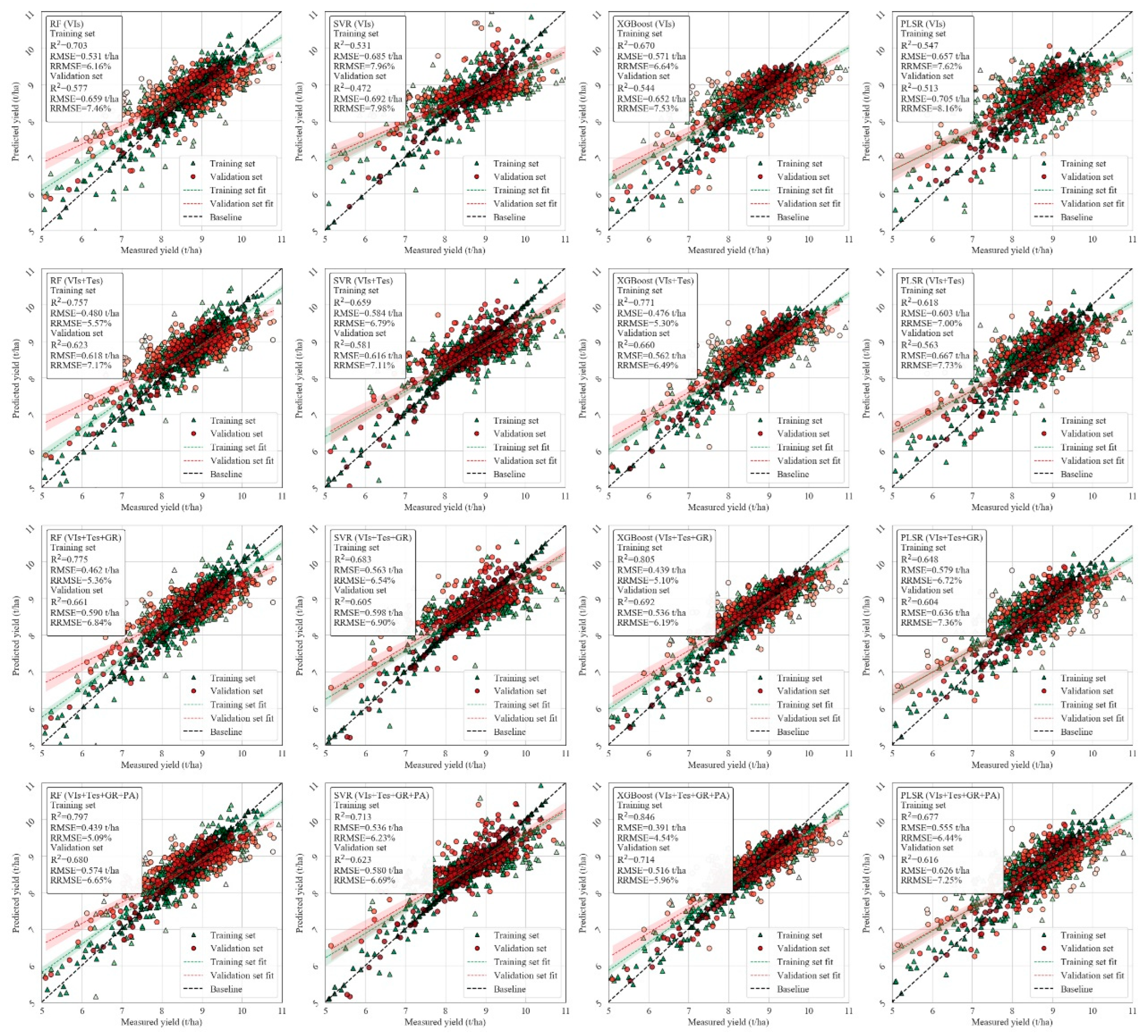
The fitted results shown in Figure 9 indicate that prediction accuracy improved progressively as more feature types were incorporated. Models using only VIs exhibited limited predictive power, whereas the addition of texture parameters markedly enhanced accuracy, especially for medium and high yield plots. Further integration of GR and PA produced additional, though more modest, gains in accuracy. At this stage, scatter points were closely aligned with the 1:1 reference line across all yield ranges, and consistency between the training and validation sets was substantially strengthened.
With respect to algorithm performance, nonlinear ensemble methods demonstrated clear advantages in high dimensional feature spaces. Among them, XGBoost consistently outperformed the other models, achieving an R2 of 0.714 on the validation set, with RMSE reduced to 0.516 t/ha and rRMSE lowered to 5.96% under the full feature combination (VIs + Tes + GR + PA). RF also performed reliably under multi-feature inputs, particularly in high yield regions. SVR suffered from underfitting when relying on single features but improved considerably with multi-source inputs. PLSR, constrained by its linear modeling framework, showed only limited gains. Overall, integrating multi-source phenotypic features substantially enhanced wheat yield prediction accuracy, and ensemble learning algorithms, particularly XGBoost, proved most effective at capturing the nonlinear contributions of growth dynamics and structural traits to yield formation.

3.5.3. Evaluation of Model Estimation Accuracy

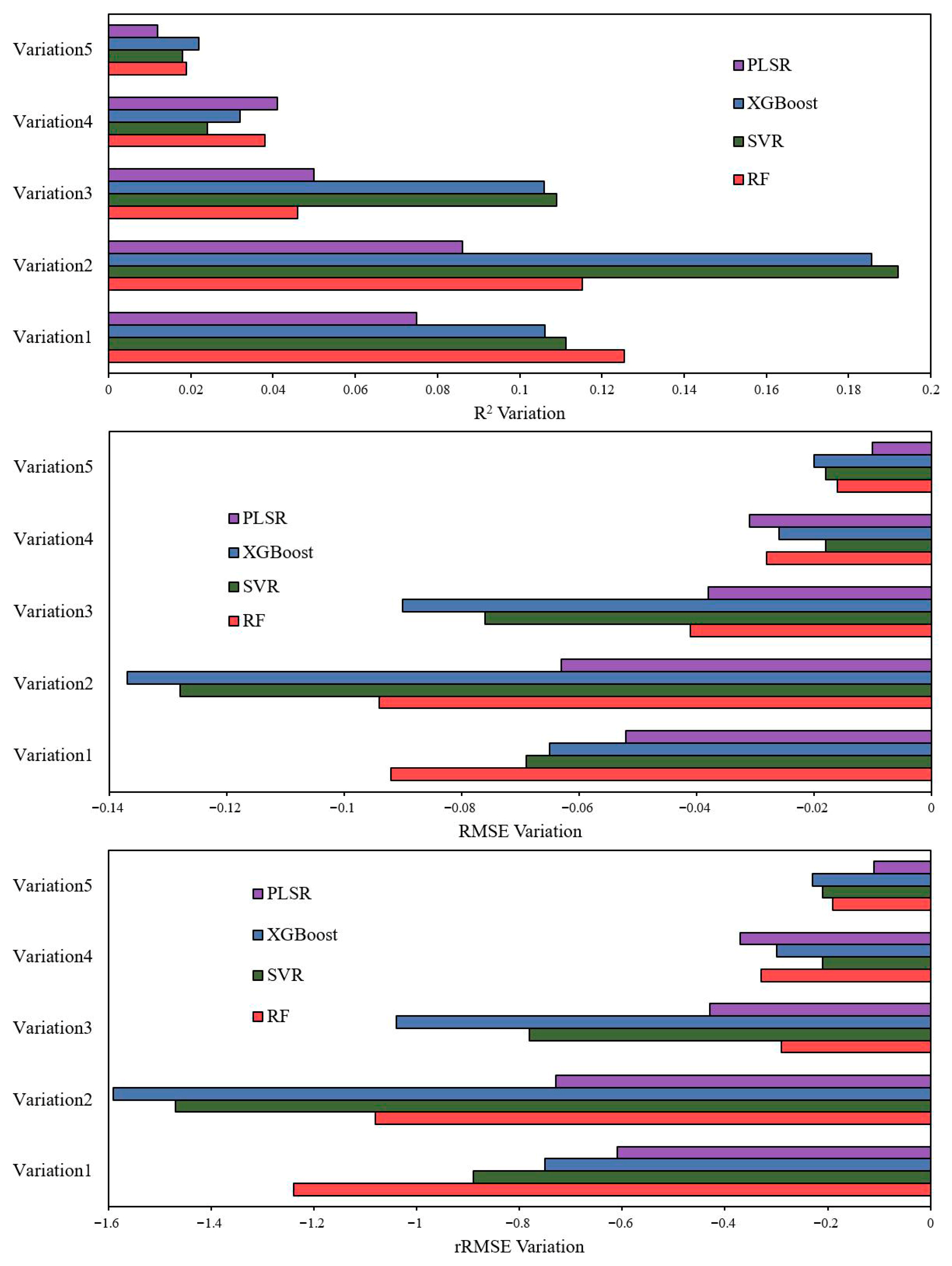
In this study, five types of feature combination variations were designed to compare model performance. Variation 1 compared models based on VIs selected from the whole growth period with those based on VIs from a single best stage. Variation 2 compared models using VIs + Tes from the whole growth period with those using the same feature set from a single best stage. Variation 3 compared VIs + Tes with VIs when both were selected from the whole growth period. Variation 4 compared VIs + Tes + GR with VIs + Tes, and Variation 5 compared VIs + Tes + GR + PA with VIs + Tes + GR, both within the whole growth period.
Figure 10 shows the differences in R2, RMSE, and rRMSE across these feature combination schemes. Overall, models based on whole growth period features consistently outperformed those using features from a single best stage. This was particularly evident in Variation 1 and Variation 2, where R2 values increased significantly, while RMSE and rRMSE decreased, indicating that multi-temporal features captured the dynamic process of yield formation more comprehensively, thereby enhancing model stability and accuracy. Within the whole growth period, Variation 3 demonstrated that the inclusion of texture parameters substantially improved model performance, with notable increases in R2 across all models and corresponding reductions in error, suggesting that texture parameters provide valuable complementary information on canopy structure and spatial heterogeneity. The strong contribution of texture features in the mid-to-late growth stages reflects the fact that genotype differences become more apparent during jointing through grain filling. Canopy uniformity, tiller synchronization, and spike emergence create distinct spatial patterns that are effectively captured by texture metrics, offering structural cues that are not fully represented by spectral indices alone. Furthermore, Variations 4 and 5 indicated that adding GR and PA further improved prediction accuracy. However, the incremental gains were smaller compared with the earlier feature combinations.

3.6. Yield Estimation Model Performance

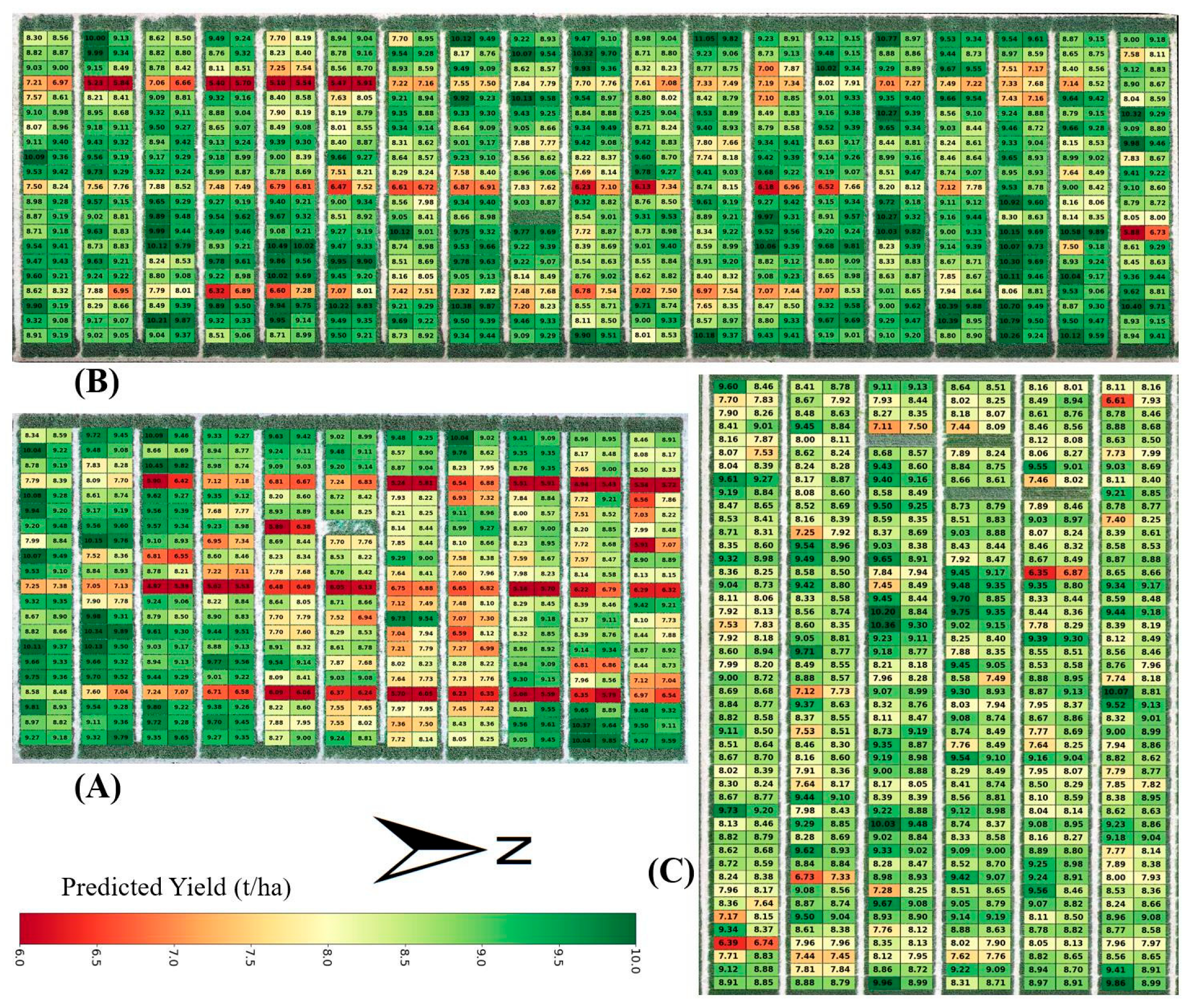
Using the best performing model, XGBoost with the full feature combination, yield estimation was conducted for the three fields, and plot scale inversion results were obtained (Figure 11). Colors from low to high correspond to a yield range of 6.0–10.0 t/ha. Overall, Field C displayed a continuous and uniform spatial pattern, with most plots concentrated between 8.0 and 9.5 t/ha, only a few scattered medium and low yield patches, and a relatively small degree of dispersion. A visually more compact distribution pattern was observed in Field C, suggesting lower apparent variability at the plot level. This visual pattern is consistent with the expected population uniformity of mature registered varieties, although no formal spatial autocorrelation analysis was conducted. In contrast, Field A and Field B exhibited more pronounced patchiness and heterogeneity, with alternating high and low yield plots frequently occurring within the same row or column. Low yield and medium to high yield plots were interspersed, highlighting the spatial expression of genetic differences and canopy structural variation among breeding materials. Overall, these results demonstrate that multi-source and multi-temporal feature integration enables effective capture of subtle yield differences at the plot scale. From a breeding perspective, such spatial distribution maps can be directly used to locate superior lines, identify problematic areas, and provide intuitive guidance for subsequent field inspections and decision making.

4. Discussion

4.1. Challenges and Opportunities in Wheat Breeding: The Role of UAV-Based Phenotyping

Wheat is a cornerstone crop for global food security, yet its breeding process, from early-stage line selection to the evaluation of officially registered varieties, remains labor-intensive and time-consuming [49]. Traditional phenotypic assessment relies heavily on manual observation, which faces several limitations [50]. Early-stage breeding programs must evaluate thousands of lines, making comprehensive and objective trait assessment difficult due to restricted labor capacity and observer subjectivity. In later stages, registered varieties require multi-environment and multi-year trials to verify yield, quality, and resistance stability, further increasing workload and environmental dependency. Moreover, yield and grain quality can only be measured accurately at harvest, leaving a lack of real-time indicators to support early selection, thereby extending the breeding cycle and reducing decision-making efficiency.
As modern breeding increasingly demands high-throughput, continuous, and precise phenotypic monitoring, technologies capable of tracking developmental trajectories from emergence to maturity have become essential [51,52]. UAV-based phenotyping provides a promising solution by rapidly acquiring large-scale spectral and structural data and extracting canopy traits and growth dynamics. Such capabilities allow quantitative assessment of population uniformity, growth rhythm, and yield potential [53,54]. Compared with traditional approaches, UAV-based monitoring shortens the trait acquisition cycle and supplies predictive information before harvest, offering more efficient and reliable support for both early-stage screening and registered variety evaluation.

4.2. Interpretation of Phenotypic Indicators and Growth Dynamics

Our results showed that multi-temporal phenotypic indicators captured the growth differences among breeding lines and registered cultivars in a complementary manner. First, vegetation indices consistently ranked among the most important predictors, particularly those related to the red-edge and near-infrared regions [19,55]. Their strong contribution aligns with the physiological basis of yield formation: leaf area expansion, chlorophyll accumulation, and sustained photosynthetic capacity during the jointing–grain filling period. This explains why models using later-stage VIs achieved markedly higher accuracy in our study, consistent with previous findings that VIs become more yield-informative as canopy biomass and pigment concentration peak [56].
Texture features further enhanced model performance, especially in early breeding materials. Our results indicated that indices such as contrast, entropy, and homogeneity significantly improved prediction accuracy when combined with VIs. This reflects the fact that breeding lines exhibited higher spatial heterogeneity, including uneven tillering, variable canopy closure, and inconsistent plant height, whereas registered cultivars showed more uniform canopy structures. Similar observations have been reported in wheat phenotyping studies where canopy structural uniformity is linked to improved light distribution and yield potential [57,58,59,60]. Dynamic canopy height traits introduced an additional dimension by quantifying differences in growth rhythm. Logistic-derived parameters (Dx, M, Dy) were more dispersed among early breeding lines, indicating variability in developmental transitions, whereas registered cultivars exhibited concentrated and synchronized growth curves. This finding supports the notion that growth rate and developmental timing are intrinsic genetic attributes influencing sink–source balance, as also noted in high-throughput phenotyping studies using height trajectories [29,61].
Together, these patterns suggest that spectral traits primarily capture biochemical processes, texture traits reflect spatial structural organization, and height dynamics describe temporal developmental rhythm. Their combined use aligns closely with the biological determinants of yield, offering a more holistic characterization of genotype performance than any single phenotypic dimension.

4.3. Differences in the Model Performance

The performance differences among the four algorithms under various feature and temporal configurations reflect their distinct abilities to represent nonlinear patterns, capture high-level feature interactions, and utilize temporal information. Across all scenarios, XGBoost consistently achieved the highest accuracy, which is consistent with previous UAV-based phenotyping studies reporting its superior capability for modeling complex crop traits and yield outcomes [32]. Its advantage arises from two main factors. First, gradient boosting can model high-order interactions between spectral and structural traits—such as the combined effects of red-edge VIs, NIR-derived indices, texture contrast, and entropy—which are known to drive phenotypic variation in canopy physiology. Second, its regularized additive structure prevents overfitting in high-dimensional, correlated feature spaces, enabling robust generalization [62,63].
RF generally performed second best across scenarios, indicating that out-of-bag sampling and multi-tree averaging effectively reduce variance, but its capacity to leverage weak signals and fine grained interactions was inferior to the boosting framework [64]. SVR showed limited performance with single feature sets due to kernel and hyperparameter scalability issues, but its performance improved markedly with richer features, underscoring its sensitivity to feature engineering quality [65]. PLSR alleviated multicollinearity through latent variables, yet remained essentially a linear approximation, making it less capable of capturing saturation, threshold, and interaction-driven nonlinear responses, thereby yielding limited improvement [66]. From a breeding perspective, these differences in model performance highlight their suitability for different application scenarios. Nonlinear ensemble models are better aligned with the complex relationships among genotype, phenotype, and yield in breeding populations, and their broader adoption will provide critical support for precision breeding driven by large scale phenotypic data.
The comparison between stage-specific and whole growth period modeling reveals an information–stability trade-off. Stage-specific models performed best during grain filling, a pattern also documented in earlier UAV studies, because this period corresponds to peak LAI, chlorophyll accumulation, and active grain biomass deposition, making VIs most strongly associated with yield [67,68]. In contrast, models built around early jointing stages underperformed due to insufficient canopy structural development and weak phenotypic expression. Whole growth period feature integration enhanced robustness, as seen in Variations 1 and 2, by aggregating cumulative signals related to growth dynamics and yield formation [69]. The complementary roles of spectral and texture features explain the substantial improvement in Variation 3. Texture metrics mitigate the saturation of VIs at late stages by capturing canopy structural heterogeneity, a phenomenon widely reported in wheat and maize studies [21,38]. GR and PA contributed smaller gains (Variations 4 and 5) because they partially overlap with static features in the information they provide, but their inclusion still improved model stability, confirming previous findings that growth-curve–derived traits provide structural priors that refine yield estimation [70].
At the level of feature contributions, the stable importance of red-edge indices, near-infrared indices, and texture metrics such as contrast, entropy, and homogeneity in the mid-to-late growth stages is consistent with physiological expectations. Differences in error structures are also noteworthy. The scatterplots indicate that extreme high yield and low yield samples are more prone to systematic deviations, manifesting as underestimation at the high yield end and overestimation at the low yield end, a typical shrinkage effect [71]. The averaging mechanism of RF exacerbates this bias in the high yield tail, whereas XGBoost, through fine grained leaf node partitioning and asymmetric loss adjustment, can partially mitigate the issue. Collectively, these findings reinforce that nonlinear ensemble learning models, especially XGBoost, are well suited for capturing the intricate genotype–phenotype–yield relationships typical in large-scale breeding populations. Their adoption can therefore substantially enhance the predictive power of UAV-based phenotyping pipelines and support more accurate and efficient decision making in wheat breeding programs.
Although the multi-temporal UAV-based approach achieved relatively high accuracy, several practical limitations should be recognized. UAV data acquisition is inherently sensitive to weather conditions, particularly wind, cloud cover, and rapid changes in illumination, all of which may introduce noise into spectral measurements. Flight-time and battery constraints can limit the area that can be covered within a single mission, potentially increasing temporal gaps among plots. Radiometric differences caused by varying solar angles, sensor drift, or inconsistent calibration settings can also influence reflectance values across dates. Furthermore, temporal inconsistencies among flight campaigns may introduce phenological discrepancies, especially during rapid growth periods. Acknowledging these operational constraints provides appropriate context for interpreting the achieved accuracy and highlights areas where future improvements in standardization and automation can further stabilize UAV-based phenotyping.

4.4. Practical Implications and Future Prospects

The findings of this study offer direct and actionable value for wheat breeding practice. First, multi-temporal UAV phenotypic indicators, including VIs, texture parameters, canopy height, and logistic-derived dynamic parameters, enable accurate yield prediction before harvest. This allows breeders to identify promising or poor-performing lines in advance rather than waiting for final yield measurements, thereby accelerating early-stage elimination and advancement decisions. Second, structural traits derived from growth dynamics reveal key attributes such as population uniformity and developmental rhythm, which traditionally rely heavily on subjective field judgment. With these objective metrics, breeders can more reliably select genotypes characterized by coordinated growth and strong adaptability, while also detecting problematic lines at an earlier stage. Third, the spatial yield maps generated in this study provide intuitive guidance for field inspection and verification. They allow breeders to locate abnormal plots, identify management issues, or detect areas where genotype performance is unstable, ultimately improving the efficiency of field trial management.
For registered cultivars and regional trials, the proposed multi-source modeling framework can be used to assess performance stability across different fields, supporting evaluations of uniformity, stability, and adaptability. This provides quantitative evidence for variety registration and demonstration. Looking ahead, the integration of hyperspectral imaging, LiDAR, thermal sensing, and advanced deep learning or time-series modeling techniques will enable UAV phenotyping platforms to capture crop physiological and structural traits with greater precision [72,73,74]. Reliable multi-source phenotypic data obtained from UAV platforms forms a fundamental component of modern AI-driven digital agriculture. Advanced machine learning and deep learning systems require consistent, high-quality inputs to accurately describe crop physiology, spatial variation, and yield formation. The multi-temporal indicators in this study, including spectral indices, canopy structural traits, and logistic-derived growth dynamics, provide a well-organized dataset that meets the data needs of contemporary prediction models. By capturing growth trajectories and genotype-dependent canopy patterns with high temporal resolution, the study shows how UAV phenotyping can enhance model interpretability, stability, and predictive performance. Such data-centered workflows are increasingly important as digital agriculture moves toward intelligent decision-making and precision breeding. Overall, the continuous maturation of UAV-based phenotyping technologies, together with advances in algorithmic modeling, is paving an efficient, precise, and scalable path for intelligent wheat breeding, with promising potential to play a greater role in crop improvement and global food security.

5. Conclusions

This study set out to determine whether multi-temporal UAV phenotyping can accurately characterize wheat growth dynamics and support yield estimation for both breeding lines and registered cultivars. The results confirm that vegetation indices, texture parameters, and canopy height traits captured complementary aspects of wheat development across the growing season and revealed clear differences in developmental rhythm and canopy uniformity among genotype groups. Dynamic parameters derived from logistic growth curves provided additional information about critical phases of growth, demonstrating that temporal structural traits can strengthen phenotypic interpretation beyond conventional static indicators.
In evaluating yield prediction, the integration of spectral, textural, and structural features consistently enhanced model performance. The XGBoost model using the full feature combination achieved the highest accuracy on the validation set, reaching an R2 of 0.714, an RMSE of 0.516 t/ha, and an rRMSE of 5.96%, confirming the effectiveness of multi-source fusion for yield estimation. The findings verify that cross-stage information improves robustness compared with single-stage modeling and that structural features such as growth rate and projected area provide measurable contributions to prediction accuracy. More broadly, this study shows that UAV-based phenotyping can support modern automated breeding workflows. The multi-temporal indicators provide quantitative inputs for machine learning-assisted trait scoring, enable earlier identification of promising genotypes before harvest, and facilitate large-scale yield evaluation with reduced labor. The proposed framework thus offers a practical foundation for integrating high-throughput phenotyping into data-driven breeding systems.

Author Contributions

Conceptualization, L.L. and X.Z. (Xinxing Zhou); methodology, T.L. and J.L.; software, X.Z. (Xinxing Zhou) and X.Z. (Xuecheng Zhu); formal analysis, N.Z. and J.W.; investigation, Y.Y. and H.Z.; resources, G.F.; data curation, T.L. and X.Z. (Xinxing Zhou); writing—original draft preparation, L.L. and X.Z. (Xinxing Zhou); writing—review and editing, H.M.; supervision, D.L.; project administration, D.L. and H.M.; funding acquisition, D.L. All authors have read and agreed to the published version of the manuscript.

Funding

This research was funded by the China Agricultural Research System (CARS-03) and Xuzhou Science and Technology Project (KC23124).

Data Availability Statement

The data presented in this study are available upon request from the corresponding author.

Conflicts of Interest

The authors declare that there are no conflicts of interest.

References

  1. Tester, M.; Langridge, P. Breeding technologies to increase crop production in a changing world. Science 2010, 327, 818–822. [Google Scholar] [CrossRef]
  2. Yu, N.; Li, L.; Schmitz, N.; Tian, L.F.; Greenberg, J.A.; Diers, B.W. Development of methods to improve soybean yield estimation and predict plant maturity with an unmanned aerial vehicle based platform. Remote Sens. Environ. 2016, 187, 91–101. [Google Scholar] [CrossRef]
  3. Breseghello, F.; Coelho, A.S.G. Traditional and modern plant breeding methods with examples in rice (Oryza sativa L.). J. Agric. Food. Chem. 2013, 61, 8277–8286. [Google Scholar] [CrossRef]
  4. Zhou, J.; Yungbluth, D.; Vong, C.N.; Scaboo, A.; Zhou, J. Estimation of the maturity date of soybean breeding lines using UAV-based multispectral imagery. Remote Sens. 2019, 11, 2075. [Google Scholar] [CrossRef]
  5. Ranđelović, P.; Đorđević, V.; Milić, S.; Balešević-Tubić, S.; Petrović, K.; Miladinović, J.; Đukić, V. Prediction of soybean plant density using a machine learning model and vegetation indices extracted from RGB images taken with a UAV. Agronomy 2020, 10, 1108. [Google Scholar] [CrossRef]
  6. Curtis, T.; Halford, N.G. Food security: The challenge of increasing wheat yield and the importance of not compromising food safety. Ann. Appl. Biol. 2014, 164, 354–372. [Google Scholar] [CrossRef] [PubMed]
  7. Mujeeb-Kazi, A.; Kazi, A.G.; Dundas, I.; Rasheed, A.; Ogbonnaya, F.; Kishii, M.; Bonnett, D.; Wang, R.R.; Xu, S.; Chen, P. Genetic diversity for wheat improvement as a conduit to food security. Adv. Agron. 2013, 122, 179–257. [Google Scholar]
  8. Novoselović, D.; Drezner, G.; Lalić, A. Contribution of wheat breeding to increased yields in Croatia from 1954. to 1985. Year. Cereal Res. Commun. 2000, 28, 95–99. [Google Scholar] [CrossRef]
  9. Reynolds, M.P.; Slafer, G.A.; Foulkes, J.M.; Griffiths, S.; Murchie, E.H.; Carmo-Silva, E.; Asseng, S.; Chapman, S.C.; Sawkins, M.; Gwyn, J. A wiring diagram to integrate physiological traits of wheat yield potential. Nat. Food 2022, 3, 318–324. [Google Scholar] [CrossRef]
  10. Pour-Aboughadareh, A.; Kianersi, F.; Poczai, P.; Moradkhani, H. Potential of wild relatives of wheat: Ideal genetic resources for future breeding programs. Agronomy 2021, 11, 1656. [Google Scholar] [CrossRef]
  11. Wang, L.; Zheng, Y.; Duan, L.; Wang, M.; Wang, H.; Li, H.; Li, R.; Zhang, H. Artificial selection trend of wheat varieties released in Huang-Huai-Hai region in China evaluated using DUS testing characteristics. Front. Plant Sci. 2022, 13, 898102. [Google Scholar] [CrossRef]
  12. Gonzalez-Dugo, V.; Hernandez, P.; Solis, I.; Zarco-Tejada, P.J. Using high-resolution hyperspectral and thermal airborne imagery to assess physiological condition in the context of wheat phenotyping. Remote Sens. 2015, 7, 13586–13605. [Google Scholar] [CrossRef]
  13. Jin, X.; Zarco-Tejada, P.J.; Schmidhalter, U.; Reynolds, M.P.; Hawkesford, M.J.; Varshney, R.K.; Yang, T.; Nie, C.; Li, Z.; Ming, B. High-throughput estimation of crop traits: A review of ground and aerial phenotyping platforms. IEEE Geosci. Remote Sens. Mag. 2020, 9, 200–231. [Google Scholar] [CrossRef]
  14. Yang, W.; Feng, H.; Zhang, X.; Zhang, J.; Doonan, J.H.; Batchelor, W.D.; Xiong, L.; Yan, J. Crop phenomics and high-throughput phenotyping: Past decades, current challenges, and future perspectives. Mol. Plant 2020, 13, 187–214. [Google Scholar] [CrossRef]
  15. Feng, L.; Chen, S.; Zhang, C.; Zhang, Y.; He, Y. A comprehensive review on recent applications of unmanned aerial vehicle remote sensing with various sensors for high-throughput plant phenotyping. Comput. Electron. Agric. 2021, 182, 106033. [Google Scholar] [CrossRef]
  16. Guo, Y.; Zhang, X.; Chen, S.; Wang, H.; Jayavelu, S.; Cammarano, D.; Fu, Y. Integrated UAV-based multi-source data for predicting maize grain yield using machine learning approaches. Remote Sens. 2022, 14, 6290. [Google Scholar] [CrossRef]
  17. Xie, C.; Yang, C. A review on plant high-throughput phenotyping traits using UAV-based sensors. Comput. Electron. Agric. 2020, 178, 105731. [Google Scholar] [CrossRef]
  18. Gitelson, A.A.; Kaufman, Y.J.; Stark, R.; Rundquist, D. Novel algorithms for remote estimation of vegetation fraction. Remote Sens. Environ. 2002, 80, 76–87. [Google Scholar] [CrossRef]
  19. Zhou, X.; Li, Y.; Sun, Y.; Su, Y.; Li, Y.; Yi, Y.; Liu, Y. Research on dynamic monitoring of grain filling process of winter wheat from time-series planet imageries. Agronomy 2022, 12, 2451. [Google Scholar] [CrossRef]
  20. Feng, D.; Yang, H.; Gao, K.; Jin, X.; Li, Z.; Nie, C.; Zhang, G.; Fang, L.; Zhou, L.; Guo, H. Time-series NDVI and greenness spectral indices in mid-to-late growth stages enhance maize yield estimation. Field Crops Res. 2025, 333, 110069. [Google Scholar] [CrossRef]
  21. Li, R.; Wang, D.; Zhu, B.; Liu, T.; Sun, C.; Zhang, Z. Estimation of nitrogen content in wheat using indices derived from RGB and thermal infrared imaging. Field Crops Res. 2022, 289, 108735. [Google Scholar] [CrossRef]
  22. Guo, Y.; Fu, Y.H.; Chen, S.; Bryant, C.R.; Li, X.; Senthilnath, J.; Sun, H.; Wang, S.; Wu, Z.; de Beurs, K. Integrating spectral and textural information for identifying the tasseling date of summer maize using UAV based RGB images. Int. J. Appl. Earth Obs. Geoinf. 2021, 102, 102435. [Google Scholar] [CrossRef]
  23. Zhou, Y.; Lao, C.; Yang, Y.; Zhang, Z.; Chen, H.; Chen, Y.; Chen, J.; Ning, J.; Yang, N. Diagnosis of winter-wheat water stress based on UAV-borne multispectral image texture and vegetation indices. Agric. Water Manag. 2021, 256, 107076. [Google Scholar] [CrossRef]
  24. Tilly, N.; Aasen, H.; Bareth, G. Fusion of plant height and vegetation indices for the estimation of barley biomass. Remote Sens. 2015, 7, 11449–11480. [Google Scholar] [CrossRef]
  25. Wang, D.; Li, R.; Zhu, B.; Liu, T.; Sun, C.; Guo, W. Estimation of wheat plant height and biomass by combining UAV imagery and elevation data. Agriculture 2022, 13, 9. [Google Scholar] [CrossRef]
  26. Yang, Y.; Li, Q.; Mu, Y.; Li, H.; Wang, H.; Ninomiya, S.; Jiang, D. UAV-assisted dynamic monitoring of wheat uniformity toward yield and biomass estimation. Plant Phenomics 2024, 6, 191. [Google Scholar] [CrossRef]
  27. Wei, L.; Yang, H.; Niu, Y.; Zhang, Y.; Xu, L.; Chai, X. Wheat biomass, yield, and straw-grain ratio estimation from multi-temporal UAV-based RGB and multispectral images. Biosyst. Eng. 2023, 234, 187–205. [Google Scholar] [CrossRef]
  28. Borra-Serrano, I.; De Swaef, T.; Quataert, P.; Aper, J.; Saleem, A.; Saeys, W.; Somers, B.; Roldán-Ruiz, I.; Lootens, P. Closing the phenotyping gap: High resolution UAV time series for soybean growth analysis provides objective data from field trials. Remote Sens. 2020, 12, 1644. [Google Scholar] [CrossRef]
  29. Tedesco, D.; de Oliveira, M.F.; Dos Santos, A.F.; Silva, E.H.C.; de Souza Rolim, G.; Da Silva, R.P. Use of remote sensing to characterize the phenological development and to predict sweet potato yield in two growing seasons. Eur. J. Agron. 2021, 129, 126337. [Google Scholar] [CrossRef]
  30. Zhang, N.; Su, X.; Zhang, X.; Yao, X.; Cheng, T.; Zhu, Y.; Cao, W.; Tian, Y. Monitoring daily variation of leaf layer photosynthesis in rice using UAV-based multi-spectral imagery and a light response curve model. Agric. For. Meteorol. 2020, 291, 108098. [Google Scholar] [CrossRef]
  31. Lee, H.; Wang, J.; Leblon, B. Using linear regression, random forests, and support vector machine with unmanned aerial vehicle multispectral images to predict canopy nitrogen weight in corn. Remote Sens. 2020, 12, 2071. [Google Scholar] [CrossRef]
  32. Zhang, P.; Lu, B.; Shang, J.; Tan, C.; Xu, Q.; Shi, L.; Jin, S.; Wang, X.; Jiang, Y.; Yang, Y. TKSF-KAN: Transformer-enhanced oat yield modeling and transferability across major oat-producing regions in China using UAV multisource data. ISPRS J. Photogramm. Remote Sens. 2025, 224, 166–186. [Google Scholar] [CrossRef]
  33. Bian, C.; Shi, H.; Wu, S.; Zhang, K.; Wei, M.; Zhao, Y.; Sun, Y.; Zhuang, H.; Zhang, X.; Chen, S. Prediction of field-scale wheat yield using machine learning method and multi-spectral UAV data. Remote Sens. 2022, 14, 1474. [Google Scholar] [CrossRef]
  34. Fei, S.; Hassan, M.A.; Xiao, Y.; Su, X.; Chen, Z.; Cheng, Q.; Duan, F.; Chen, R.; Ma, Y. UAV-based multi-sensor data fusion and machine learning algorithm for yield prediction in wheat. Precis. Agric. 2023, 24, 187–212. [Google Scholar] [CrossRef]
  35. Morlin Carneiro, F.; Angeli Furlani, C.E.; Zerbato, C.; Candida De Menezes, P.; Da Silva Gírio, L.A.; Freire De Oliveira, M. Comparison between vegetation indices for detecting spatial and temporal variabilities in soybean crop using canopy sensors. Precis. Agric. 2020, 21, 979–1007. [Google Scholar] [CrossRef]
  36. Asam, S.; Fabritius, H.; Klein, D.; Conrad, C.; Dech, S. Derivation of leaf area index for grassland within alpine upland using multi-temporal RapidEye data. Int. J. Remote Sens. 2013, 34, 8628–8652. [Google Scholar] [CrossRef]
  37. Feng, W.; Wu, Y.; He, L.; Ren, X.; Wang, Y.; Hou, G.; Wang, Y.; Liu, W.; Guo, T. An optimized non-linear vegetation index for estimating leaf area index in winter wheat. Precis. Agric. 2019, 20, 1157–1176. [Google Scholar] [CrossRef]
  38. Hall-Beyer, M. Practical guidelines for choosing GLCM textures to use in landscape classification tasks over a range of moderate spatial scales. Int. J. Remote Sens. 2017, 38, 1312–1338. [Google Scholar] [CrossRef]
  39. Sun, X.; Yang, Z.; Su, P.; Wei, K.; Wang, Z.; Yang, C.; Wang, C.; Qin, M.; Xiao, L.; Yang, W. Non-destructive monitoring of maize LAI by fusing UAV spectral and textural features. Front. Plant Sci. 2023, 14, 1158837. [Google Scholar] [CrossRef]
  40. Makanza, R.; Zaman-Allah, M.; Cairns, J.E.; Magorokosho, C.; Tarekegne, A.; Olsen, M.; Prasanna, B.M. High-throughput phenotyping of canopy cover and senescence in maize field trials using aerial digital canopy imaging. Remote Sens. 2018, 10, 330. [Google Scholar] [CrossRef] [PubMed]
  41. Weiyuan, H.; Ziqiu, L.; Xiangqian, F.; Jinhua, Q.; Aidong, W.; Shichao, J.; Danying, W.; Song, C. Estimating key phenological dates of multiple rice accessions using unmanned aerial vehicle-based plant height dynamics for breeding. Rice Sci. 2024, 31, 617–628. [Google Scholar] [CrossRef]
  42. Guo, Y.; Xiao, Y.; Li, M.; Hao, F.; Zhang, X.; Sun, H.; de Beurs, K.; Fu, Y.H.; He, Y. Identifying crop phenology using maize height constructed from multi-sources images. Int. J. Appl. Earth Obs. Geoinf. 2022, 115, 103121. [Google Scholar] [CrossRef]
  43. Wu, R.; Wang, Z.; Zhao, W.; Cheverud, J.M. A mechanistic model for genetic machinery of ontogenetic growth. Genetics 2004, 168, 2383–2394. [Google Scholar] [CrossRef]
  44. Shafiee, S.; Lied, L.M.; Burud, I.; Dieseth, J.A.; Alsheikh, M.; Lillemo, M. Sequential forward selection and support vector regression in comparison to LASSO regression for spring wheat yield prediction based on UAV imagery. Comput. Electron. Agric. 2021, 183, 106036. [Google Scholar] [CrossRef]
  45. Khodjaev, S.; Bobojonov, I.; Kuhn, L.; Glauben, T. Optimizing machine learning models for wheat yield estimation using a comprehensive UAV dataset. Model. Earth Syst. Environ. 2025, 11, 15. [Google Scholar] [CrossRef]
  46. Tao, H.; Feng, H.; Xu, L.; Miao, M.; Yang, G.; Yang, X.; Fan, L. Estimation of the yield and plant height of winter wheat using UAV-based hyperspectral images. Sensors 2020, 20, 1231. [Google Scholar] [CrossRef]
  47. Guyon, I.; Elisseeff, A. An introduction to variable and feature selection. J. Mach. Learn. Res. 2003, 3, 1157–1182. [Google Scholar]
  48. Fu, Z.; Jiang, J.; Gao, Y.; Krienke, B.; Wang, M.; Zhong, K.; Cao, Q.; Tian, Y.; Zhu, Y.; Cao, W. Wheat growth monitoring and yield estimation based on multi-rotor unmanned aerial vehicle. Remote Sens. 2020, 12, 508. [Google Scholar] [CrossRef]
  49. Martínez-Moreno, F.; Ammar, K.; Solís, I. Global changes in cultivated area and breeding activities of durum wheat from 1800 to date: A historical review. Agronomy 2022, 12, 1135. [Google Scholar] [CrossRef]
  50. Yadav, V.K.; Singh, I.S. Comparative evaluation of maize inbred lines (Zea mays L.) according to DUS testing using morphological, physiological and molecular markers. Agric. Sci. 2010, 1, 131–142. [Google Scholar] [CrossRef][Green Version]
  51. Ganeva, D.; Roumenina, E.; Dimitrov, P.; Gikov, A.; Jelev, G.; Dragov, R.; Bozhanova, V.; Taneva, K. Phenotypic traits estimation and preliminary yield assessment in different phenophases of wheat breeding experiment based on UAV multispectral images. Remote Sens. 2022, 14, 1019. [Google Scholar] [CrossRef]
  52. Peng, J.; Wang, D.; Zhu, W.; Yang, T.; Liu, Z.; Rezaei, E.E.; Li, J.; Sun, Z.; Xin, X. Combination of UAV and deep learning to estimate wheat yield at ripening stage: The potential of phenotypic features. Int. J. Appl. Earth Obs. Geoinf. 2023, 124, 103494. [Google Scholar] [CrossRef]
  53. Song, X.; Deng, Q.; Camenzind, M.; Luca, S.V.; Qin, W.; Hu, Y.; Minceva, M.; Yu, K. High-throughput phenotyping of canopy dynamics of wheat senescence using UAV multispectral imaging. Smart Agric. Technol. 2025, 12, 101176. [Google Scholar] [CrossRef]
  54. Smith, D.T.; Chen, Q.; Massey-Reed, S.R.; Potgieter, A.B.; Chapman, S.C. Prediction accuracy and repeatability of UAV based biomass estimation in wheat variety trials as affected by variable type, modelling strategy and sampling location. Plant Methods 2024, 20, 129. [Google Scholar] [CrossRef]
  55. Hassan, M.A.; Yang, M.; Rasheed, A.; Tian, X.; Reynolds, M.; Xia, X.; Xiao, Y.; He, Z. Quantifying senescence in bread wheat using multispectral imaging from an unmanned aerial vehicle and QTL mapping. Plant Physiol. 2021, 187, 2623–2636. [Google Scholar] [CrossRef] [PubMed]
  56. Ajayi, S.; Reddy, S.K.; Gowda, P.H.; Xue, Q.; Rudd, J.C.; Pradhan, G.; Liu, S.; Stewart, B.A.; Biradar, C.; Jessup, K.E. Spectral reflectance models for characterizing winter wheat genotypes. J. Crop. Improv. 2016, 30, 176–195. [Google Scholar] [CrossRef]
  57. Zhang, J.; Cheng, T.; Shi, L.; Wang, W.; Niu, Z.; Guo, W.; Ma, X. Combining spectral and texture features of UAV hyperspectral images for leaf nitrogen content monitoring in winter wheat. Int. J. Remote Sens. 2022, 43, 2335–2356. [Google Scholar] [CrossRef]
  58. Li, H.; Yan, X.; Su, P.; Su, Y.; Li, J.; Xu, Z.; Gao, C.; Zhao, Y.; Feng, M.; Shafiq, F. Estimation of winter wheat LAI based on color indices and texture features of RGB images taken by UAV. J. Sci. Food. Agric. 2025, 105, 189–200. [Google Scholar] [CrossRef] [PubMed]
  59. Zou, M.; Liu, Y.; Fu, M.; Li, C.; Zhou, Z.; Meng, H.; Xing, E.; Ren, Y. Combining spectral and texture feature of UAV image with plant height to improve LAI estimation of winter wheat at jointing stage. Front. Plant Sci. 2024, 14, 1272049. [Google Scholar] [CrossRef] [PubMed]
  60. Li, J.; Veeranampalayam-Sivakumar, A.; Bhatta, M.; Garst, N.D.; Stoll, H.; Stephen Baenziger, P.; Belamkar, V.; Howard, R.; Ge, Y.; Shi, Y. Principal variable selection to explain grain yield variation in winter wheat from features extracted from UAV imagery. Plant Methods 2019, 15, 123. [Google Scholar] [CrossRef]
  61. Tirado, S.B.; Hirsch, C.N.; Springer, N.M. UAV-based imaging platform for monitoring maize growth throughout development. Plant Direct 2020, 4, e230. [Google Scholar] [CrossRef]
  62. Han, L.; Yang, G.; Yang, X.; Song, X.; Xu, B.; Li, Z.; Wu, J.; Yang, H.; Wu, J. An explainable XGBoost model improved by SMOTE-ENN technique for maize lodging detection based on multi-source unmanned aerial vehicle images. Comput. Electron. Agric. 2022, 194, 106804. [Google Scholar] [CrossRef]
  63. Westhues, C.C.; Mahone, G.S.; Da Silva, S.; Thorwarth, P.; Schmidt, M.; Richter, J.; Simianer, H.; Beissinger, T.M. Prediction of maize phenotypic traits with genomic and environmental predictors using gradient boosting frameworks. Front. Plant Sci. 2021, 12, 699589. [Google Scholar] [CrossRef] [PubMed]
  64. Sánchez, J.C.M.; Mesa, H.G.A.; Espinosa, A.T.; Castilla, S.R.; Lamont, F.G. Improving Wheat Yield Prediction through Variable Selection Using Support Vector Regression, Random Forest, and Extreme Gradient Boosting. Smart Agric. Technol. 2025, 10, 100791. [Google Scholar] [CrossRef]
  65. Chiu, M.S.; Wang, J. Evaluation of machine learning regression techniques for estimating winter wheat biomass using biophysical, biochemical, and UAV multispectral data. Drones 2024, 8, 287. [Google Scholar] [CrossRef]
  66. Zhang, S.; He, L.; Duan, J.; Zang, S.; Yang, T.; Schulthess, U.; Guo, T.; Wang, C.; Feng, W. Aboveground wheat biomass estimation from a low-altitude UAV platform based on multimodal remote sensing data fusion with the introduction of terrain factors. Precis. Agric. 2024, 25, 119–145. [Google Scholar] [CrossRef]
  67. Dong, T.; Liu, J.; Shang, J.; Qian, B.; Ma, B.; Kovacs, J.M.; Walters, D.; Jiao, X.; Geng, X.; Shi, Y. Assessment of red-edge vegetation indices for crop leaf area index estimation. Remote Sens. Environ. 2019, 222, 133–143. [Google Scholar] [CrossRef]
  68. Hassan, M.A.; Yang, M.; Rasheed, A.; Yang, G.; Reynolds, M.; Xia, X.; Xiao, Y.; He, Z. A rapid monitoring of NDVI across the wheat growth cycle for grain yield prediction using a multi-spectral UAV platform. Plant Sci. 2019, 282, 95–103. [Google Scholar] [CrossRef]
  69. Liu, T.; Wu, F.; Mou, N.; Zhu, S.; Yang, T.; Zhang, W.; Wang, H.; Wu, W.; Zhao, Y.; Sun, C. The estimation of wheat yield combined with UAV canopy spectral and volumetric data. Food Energy Secur. 2024, 13, e527. [Google Scholar] [CrossRef]
  70. Durgun, Y.Ö.; Gobin, A.; Duveiller, G.; Tychon, B. A study on trade-offs between spatial resolution and temporal sampling density for wheat yield estimation using both thermal and calendar time. Int. J. Appl. Earth Obs. Geoinf. 2020, 86, 101988. [Google Scholar] [CrossRef]
  71. Zhang, B.; Gu, L.; Dai, M.; Bao, X.; Sun, Q.; Qu, X.; Zhang, M.; Liu, X.; Fan, C.; Gu, X. Estimation of grain filling rate and thousand-grain weight of winter wheat (Triticum aestivum L.) using UAV-based multispectral images. Eur. J. Agron. 2024, 159, 127258. [Google Scholar] [CrossRef]
  72. Zhu, X.; Liu, X.; Wu, Q.; Liu, M.; Hu, X.; Deng, H.; Zhang, Y.; Qu, Y.; Wang, B.; Gou, X. Utilizing UAV-based high-throughput phenotyping and machine learning to evaluate drought resistance in wheat germplasm. Comput. Electron. Agric. 2025, 237, 110602. [Google Scholar] [CrossRef]
  73. Sharma, V.; Honkavaara, E.; Hayden, M.; Kant, S. UAV remote sensing phenotyping of wheat collection for response to water stress and yield prediction using machine learning. Plant Stress 2024, 12, 100464. [Google Scholar] [CrossRef]
  74. Schreiber, L.V.; Atkinson Amorim, J.G.; Guimarães, L.; Motta Matos, D.; Maciel Da Costa, C.; Parraga, A. Above-ground biomass wheat estimation: Deep learning with UAV-based RGB images. Appl. Artif. Intell. 2022, 36, 2055392. [Google Scholar] [CrossRef]
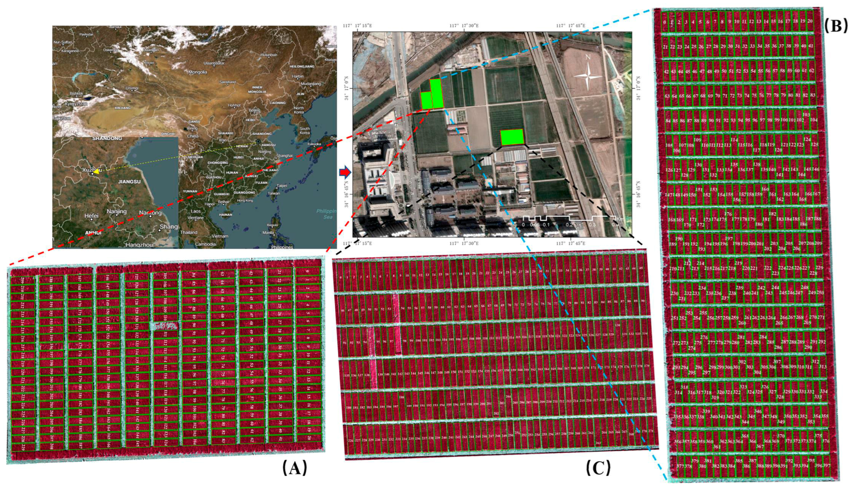
Figure 1. Location of study area. From left to right, the subfigures show the geographical location of the study area and the internal layout of the experimental station, where (AC) correspond to the three experimental fields included in this study.
Agriculture 15 02554 g001
Figure 2. The schematic diagram of data processing, model architecture. (A) UAV data acquisition and raw imagery collection across multiple wheat growth stages; (B) Extraction of VIs, texture parameters, and temporal features from multispectral, RGB, and canopy height data; (C) Whole growth period analysis, including temporal trend exploration and nonlinear growth curve fitting; (D) Construction of yield prediction models using different feature combinations and machine-learning algorithms; (E) Model evaluation using predicted and measured yield with R2, RMSE, and rRMSE; (F) Ground truth yield measurements collected from field plots.
Agriculture 15 02554 g002
Figure 3. Examples of critical points as a function of growth curve, growth rate curve, and growth acceleration curve of VIs. Critical points represent the moment when the accelerated growth of the VIs is maximized (Dx) and minimized (Dy), M is the DAS at which the growth rate is maximized.
Agriculture 15 02554 g003
Figure 4. Distribution of yield across distinct experimental fields. Field 1 and Field 2 were planted with early-generation breeding lines, whereas Field 3 consisted of registered cultivars, all located within the same trial farm in Xuzhou, Jiangsu Province.
Agriculture 15 02554 g004
Figure 5. Changes in VIs under different growth stage. Each curve represents the mean VI value calculated from all plots within the corresponding field at each flight date. Different colors are used to distinguish Field 1, Field 2, and Field 3.
Agriculture 15 02554 g005
Figure 6. Changes in texture parameters under different growth stage. Each curve represents the mean texture value calculated from all plots within the corresponding field at each flight date. Different colors are used to distinguish Field 1, Field 2, and Field 3.
Agriculture 15 02554 g006
Figure 7. Logistic growth curves of canopy height and their first- and second-order derivatives for wheat across three fields. Dashed lines represent individual plots, while bold solid lines denote the mean fitted curves. Dx, M, and Dy indicate the maximum growth acceleration point, the inflection point, and the minimum growth acceleration point, respectively.
Agriculture 15 02554 g007
Figure 8. Feature importance ranking and cumulative contribution of spectral and texture features for wheat yield estimation. The numbers following each feature name (1–7) indicate the growth stage at which the feature was extracted, corresponding to the seven UAV flight periods (from overwintering to grain filling). Features with the same abbreviation but different numbers represent measurements acquired at different growth stages.
Agriculture 15 02554 g008
Figure 9. Comparison of yield estimation performance among RF, SVR, XGBoost, and PLSR models using VIs, VIs + Tes, VIs + Tes + GR, and VIs + Tes + GR + PA feature sets.
Agriculture 15 02554 g009
Figure 10. Performance variations in different feature combinations across four modeling algorithms evaluated by R2, RMSE, and Rrmse.
Agriculture 15 02554 g010
Figure 11. Spatial distribution of plot-level wheat yield estimation across three fields using the XGBoost model with full feature combinations. (A), (B), and (C) correspond to fields containing 230, 398, and 272 plots, respectively. Each experimental plot displays two numerical values: the left value indicates the measured grain yield obtained through manual harvesting at crop maturity, and the right value indicates the estimated yield generated by the XGBoost model. Color gradients represent the spatial variation in estimated yield (t/ha), with darker green indicating higher productivity and red indicating lower productivity.
Agriculture 15 02554 g011
Table 1. Vegetation indices and its calculation formula.
AbbreviationFull NameFormula
NDVINormalized difference vegetation index(NIR − Red)/(NIR + Red)
GNDVIGreen normalized difference vegetation index(NIR − Green)/(NIR + Green)
RVIRatio vegetation indexNIR/Red
DVIDifference vegetation indexNIR − Red
NDRENormalized difference red edge index(NIR − Red_edge)/(NIR + Red_edge)
NDVI_redgNormalized difference vegetation index red-edge(Red_edge − Red)/(Red_edge + Red)
NRINitrogen reflectance index(Green − Red)/(Green + Red)
SAVISoil adjusted vegetation index1.5 (NIR − Red)/(NIR + Red + 0.5)
Note: Green, red, Red_edge and NIR denoted spectral reflectance at green, red, red-edge and near-infrared bands, respectively.
Table 2. Texture parameters and its calculation formula.
AbbreviationFull NameFormula
MEAMean Σ i , j N 1 i P i , j
VARVariance Σ i , j = 0 N 1 i P i , j i m e a n 2
HOMHomogeneity i , j = 0 N 1 i P i , j 1 + j 2
CONContrast Σ i , j = 0 N 1 i P i , j i j 2
DISDissimilarity Σ i , j = 0 N 1 i P i , j i j
ENTEntropy Σ i , j = 0 N 1 i P i , j ( l n P i , j )
SECSecond moment Σ i , j = 0 N 1 i P i , j 2
CORCorrelation i , j = 0 N 1 i P i , j i m e a n j m e a n v a r i a n c e i × v a r i a n c e j
Note: P i , j = V i , j Σ i , j = 0 N 1 V i , j Vi,j denotes the brightness value of the pixel located at the i-th row and j-th column, and N represents the size of the moving window used for calculating the texture measures.
Table 3. Model performance for wheat yield estimation using vegetation indices at different growth stages.
Growth StageModelTraining Set R2Validation Set R2Training Set RMSE (t/ha)Validation Set RMSE (t/ha)Training Set rRMSEValidation Set rRMSE
Overwintering stageRF0.3190.1660.8040.9269.32%10.74%
SVR0.1430.0950.9260.90510.76%10.45%
XGBoost0.3630.2460.7940.8389.23%9.68%
PLSR0.1370.130.9060.94210.52%10.91%
Regreening stageRF0.2180.120.8610.9519.99%11.02%
SVR0.1140.0730.9410.91610.94%10.57%
XGBoost0.3780.2520.7850.8359.12%9.64%
PLSR0.10.0840.9260.96610.74%11.19%
Jointing stageRF0.1370.080.9040.97210.49%11.27%
SVR0.1260.0810.9350.91210.87%10.53%
XGBoost0.2720.1730.8480.8779.86%10.13%
PLSR0.0710.0450.9410.98610.91%11.43%
Booting stageRF0.0670.0480.9410.98910.91%11.47%
SVR0.0740.0350.9620.93411.18%10.78%
XGBoost0.2730.1690.8480.889.85%10.16%
PLSR0.0750.0530.9380.98310.89%11.38%
Heading stageRF0.2990.1690.8150.9249.46%10.71%
SVR0.170.1110.9110.89710.59%10.35%
XGBoost0.3670.2710.7910.8249.19%9.51%
PLSR0.210.1570.8670.92710.06%10.74%
Flowering stageRF0.4470.3270.7240.8328.40%9.64%
SVR0.230.1820.8770.8610.20%9.93%
XGBoost0.4540.3340.7350.7878.54%9.09%
PLSR0.3170.2520.8060.8919.36%10.32%
Grain filling stageRF0.530.4520.6670.7517.74%8.70%
SVR0.420.3610.7610.7618.85%8.78%
XGBoost0.570.4480.6520.7177.57%8.28%
PLSR0.45590.4380.720.7578.35%8.77%
Table 4. Model performance for wheat yield estimation using vegetation indices and texture parameters at different growth stages.
Growth StageModelTraining Set R2Validation Set R2Training Set RMSE (t/ha)Validation Set RMSE (t/ha)Training Set rRMSEValidation Set rRMSE
Overwintering stageRF0.3460.20.7880.9079.14%10.51%
SVR0.1850.1570.9030.87410.49%10.08%
XGBoost0.3910.2620.7760.8299.02%9.57%
PLSR0.2770.1990.830.9039.63%10.46%
Regreening stageRF0.3240.1840.8010.9169.29%10.62%
SVR0.1420.1210.9260.89210.77%10.30%
XGBoost0.40.2770.770.828.95%9.48%
PLSR0.2240.1640.8590.9239.97%10.69%
Jointing stageRF0.3640.210.7770.9019.01%10.44%
SVR0.1790.1160.9060.89410.53%10.32%
XGBoost0.3550.2070.7990.8599.28%9.92%
PLSR0.2240.1610.8690.92410.07%10.71%
Booting stageRF0.2780.1540.8280.9339.60%10.81%
SVR0.1250.0870.9360.90910.87%10.49%
XGBoost0.3270.1890.8160.8699.48%10.03%
PLSR0.1050.0810.9330.96810.81%11.21%
Heading stageRF0.380.2570.5240.8746.08%10.13%
SVR0.1860.1290.9020.88810.48%10.25%
XGBoost0.4880.3390.7120.7848.27%9.06%
PLSR0.2790.2020.8290.9029.61%10.45%
Flowering stageRF0.4920.3690.6940.8068.05%9.34%
SVR0.3520.2210.8050.849.36%9.69%
XGBoost0.5290.40.6830.7487.93%8.63%
PLSR0.3910.3140.7610.8368.84%9.68%
Grain filling stageRF0.6190.5080.6010.7116.98%8.25%
SVR0.4440.3890.7450.7448.66%8.58%
XGBoost0.6070.4750.6240.6997.25%8.08%
PLSR0.5050.4770.6870.737.97%8.46%
Disclaimer/Publisher’s Note: The statements, opinions and data contained in all publications are solely those of the individual author(s) and contributor(s) and not of MDPI and/or the editor(s). MDPI and/or the editor(s) disclaim responsibility for any injury to people or property resulting from any ideas, methods, instructions or products referred to in the content.