A Study on Digital Soil Mapping Based on Multi-Attention Convolutional Neural Networks: A Case Study in Heilongjiang Province

Abstract

Machine learning-based digital soil mapping often struggles with spatial heterogeneity and long-range dependencies. To address these limitations, this study proposes Multi-Attention Convolutional Neural Networks (MACNN). This deep learning algorithm integrates multiple attention mechanisms to improve mapping accuracy. First, environmental covariates are determined from the soil-landscape model. These are then fed as structured input to the Convolutional Neural Network. Next, by incorporating Transformer self-attention and multi-head attention mechanisms, this study effectively models the long-range dependencies between soil types and features. Concurrently, the Convolutional Block Attention Module (CBAM) is introduced. CBAM features both channel and spatial dual attention, enabling adaptive weighting of crucial feature channels and spatial locations. This significantly enhances the algorithm’s sensitivity to discriminative information. To validate its effectiveness, the proposed MACNN algorithm was used for soil type mapping in Heilongjiang Province. Compared to Random Forest, Decision Tree, and One-Dimensional Convolutional Neural Network algorithms, MACNN demonstrated superior classification performance. It achieved an overall classification accuracy of 81.27%. An ablation study was conducted to investigate the importance of individual modules within the proposed algorithm. The findings indicate that progressively integrating Transformer and CBAM modules into the 1D-CNN baseline significantly enhances algorithm performance through synergistic gains. Therefore, this integrated algorithm offers a feasible solution to improve digital soil mapping accuracy, providing significant reference value for future research and applications.

1. Introduction

As the foundation of terrestrial ecosystems, soil plays an irreplaceable role in global ecological balance, food security, and climate change mitigation. However, the combined effects of climate change and agricultural intensification are causing structural changes in soil type composition. This shift threatens the sustainable use of soil resources and poses significant challenges to agricultural production and ecological environment management [1]. High-accuracy digital soil maps are vital for efficient soil resource management. They also enable the precise allocation of soil conservation and management technologies. The core principle of Digital Soil Mapping (DSM) involves utilizing soil survey data alongside specific soil-forming factors. These factors are either directly linked to soil formation or exhibit spatially co-varying relationships with soil properties [2]. High-accuracy digital soil maps are then inferred and generated using methods such as statistical modeling, machine learning, or geostatistics [3]. Based on the distinct core methodologies algorithms employ to establish soil–environment relationships, DSM can be categorized into data-driven machine learning (ML) algorithms [4], such as Random Forest (RF) [5], Decision Tree (DT) [6], Support Vector Machine (SVM) [7], and Neural Networks (NN) [8]. Furthermore, it includes statistical algorithms with explicit mathematical models [9], exemplified by Kriging; expert knowledge-based algorithms that rely on prior rules and empirical experience; and sample point representativeness algorithms [10] that infer from environmental similarity, such as the Soil-Landscape Unit method. Among these, machine learning algorithms are capable of mining the nonlinear relationships between soil and soil-forming factors, thereby enabling the prediction and spatial mapping of soil types in unsampled areas. Consequently, they are widely applied in digital soil mapping [11]. Chen R. et al. [5] predicted the spatial distribution of soil types by utilizing multi-temporal remote sensing images in conjunction with the Random Forest (RF) algorithm. KOVAČEVIĆ et al. [12] utilized Support Vector Machines (SVM) to model and analyze soil types, soil organic matter (SOM) content, and pH values in the eastern region of Serbia. Nauaf et al. [13] utilized RGB values from remote sensing imagery to estimate soil organic matter content. Song Q. et al. [14] calculated soil organic carbon content using hyperspectral imagery. However, soil formation processes are governed by the complex nonlinear coupling of multiple factors, including climate, organisms, and topography. While traditional machine learning algorithms excel in nonlinear feature identification and extraction, they often lack the perceptive ability to handle the spatial heterogeneity inherent in complex data and struggle to simulate the dynamic processes of soil evolution. Consequently, it is challenging for them to achieve significant improvements in mapping accuracy. Algorithms like Decision Trees, which build hierarchical rules, and Random Forests, an ensemble method, exemplify these limitations. While effective for feature-based learning, their architectures struggle with explicit spatial or temporal pattern recognition, often relying on flat feature representations.

Compared to traditional machine learning algorithms, Deep Learning (DL) algorithms perform hierarchical abstraction and representation learning on input data through multi-layer neural networks [15]. This enables them to be more adept at handling complex features and large-scale data, effectively perceive the spatial heterogeneity of complex data, and consequently improve classification accuracy and generalization ability. The application of DL in digital soil mapping is steadily increasing, establishing it as a significant research hotspot and future direction in the field. Among various DL architectures, Convolutional Neural Networks (CNN) are particularly prominent. WADOUX et al. [16] employed CNN for the spatial prediction mapping of soil organic carbon (SOC) content. PADARIAN et al. [17] utilized a CNN algorithm to predict six types of soil attributes, based on the LUCAS dataset. Their results indicated that CNN demonstrated good performance in soil attribute prediction. Despite the widespread application of CNNs in DSM, it has been revealed through ongoing research that CNN architectures suffer from the limitation of local connectivity, which prevents them from effectively capturing long-range dependencies between features. To enhance algorithm performance, Sun et al. [18] integrated a CBAM into the CNN architecture, aiming to optimize the local receptive field and improve computational efficiency. However, under complex topographic conditions, this approach demonstrated limited capability in recognizing long-range dependencies among soil-forming factors. Guo et al. [19] utilized attention mechanisms to enable dynamic focusing on crucial regions; yet, a challenge arose in dealing with multi-level features, where an imbalance in feature response was observed. In summary, current DSM algorithms still face challenges in effectively integrating the long-range dependencies between soil-forming factors that govern soil genesis and distribution and in extracting sufficiently discriminative features from complex multi-source data. These limitations directly compromise the accuracy of soil type classification and the overall quality of DSM.

In light of these identified limitations, this study, by following the theoretical framework of digital soil mapping and the soil-landscape SCORPAN model [20], initially derived the relationships between soil types and soil-forming factors [21]. This experiment aims to develop an enhanced fine-grained soil type classification approach that addresses the inherent limitations of current methodologies. Building upon this, a novel MACNN algorithm is proposed. This algorithm introduces various attention mechanisms into the CNN architecture to address the challenges faced by existing digital soil mapping algorithms in handling spatial heterogeneity and long-range dependencies, ultimately enhancing the fine-grained classification capability of soil types. Taking soil type mapping in Heilongjiang Province as a case study, the classification results of the proposed algorithm were compared with those from RF, DT, and a 1D-CNN. Furthermore, an ablation study was conducted to comprehensively evaluate the applicability of this algorithm in soil type mapping, with the aim of providing novel technical support for digital soil mapping.

2. Materials and Methods

2.1. Description of the Study Area

Heilongjiang Province, located in Northeast China, is the country’s northernmost and highest-latitude province, spanning geographic coordinates from 121°11′ E to 135°05′ E and 43°26′ N to 53°33′ N (Figure 1). The region exhibits complex topography, with higher elevations in the northwest, north, and southeast, and lower elevations in the east and southwest. The terrain is primarily composed of mountains, platforms (or tablelands), plains, and water bodies. Land use types are predominantly cultivated land and forests. Key soil parent materials include granite, gneiss, and basalt, among others. The climate displays significant regional variations; precipitation, influenced by the monsoon climate, differs considerably across various regions and seasons, with concentrated rainfall in summer and relatively dry winters. Owing to the diversity in geographical and climatic conditions, the province hosts 19 distinct soil types, which show significant spatial distribution differences. Therefore, the diverse soil types, complex parent materials, and variable climatic conditions of Heilongjiang Province make it a highly representative region for investigating the influence of environmental factors on soil formation.

2.2. Data Collection and Preprocessing

2.2.1. Soil Sample Data

The acquisition of soil sample data was conducted in strict accordance with established soil survey guidelines. Representative soil profile points were strategically selected and established, with high-precision GPS devices utilized to meticulously record the latitude, longitude, and elevation data for each profile. During field investigations, each soil profile underwent detailed excavation and comprehensive description. Key morphological characteristics, such as color and texture, were meticulously documented for each horizon. Subsequently, laboratory physicochemical analyses were performed to ascertain the definitive soil type and attribute information.

The Second National Soil Survey Map of China was delineated and produced by soil experts, with the support of the soil-landscape model. Consequently, it incorporates valuable prior knowledge and exhibits high mapping accuracy. The high cost of field investigations often leads to an insufficient number and spatial coverage of actual field sample points. To enhance the representativeness of the sample distribution, this study introduced virtual soil profile sample points as a complement. To ensure the scientific rigor and representativeness of these virtual points, their selection comprehensively integrated prior knowledge with information from existing field sample points. Specifically, virtual sample points were acquired through a stratified sampling method, which also considered the environmental similarity between existing and virtual points [22], ultimately defining their spatial distribution pattern and total number. By integrating 85 actual field soil profile sample points from Heilongjiang Province’s Second National Soil Survey, 410 actual field soil profile sample points [23] collected in Heilongjiang Province in 2015, and virtual soil profile sample points, a consolidated dataset of 32,920 sample points was compiled (Appendix A). This extensive dataset provides ample support for subsequent modeling and analysis.

2.2.2. Environmental Covariate Data

Soil formation processes are comprehensively influenced by multiple factors, including parent material, topography, organisms, human activities, and climate. Based on the soil-landscape SCORPAN model theory applicable to the study area, a total of 12 soil-forming factor datasets were selected. These include parent material type, topographic features (e.g., DEM, slope, aspect), Vegetation Index (NDVI), land use types, and climatic elements (e.g., air temperature, precipitation). Parent material, as the physical basis for soil formation, directly affects soil physicochemical properties through its mineral composition and weathering degree [24]. Topographic features regulate water and heat distribution and material migration, thereby shaping the spatial differentiation pattern of soils [25]. The NDVI represents vegetation cover conditions and its feedback on soil development [26]. Human activities [27], such as changes in land use patterns [28] and agricultural production practices, also profoundly impact soil properties. Furthermore, climatic elements like mean annual temperature and precipitation, along with soil texture [29], were incorporated into the indicator system to comprehensively reflect the hydrothermal conditions and material migration characteristics pertinent to soil formation (Appendix B.3).

To facilitate subsequent analysis and experimentation, the spatial resolution of the soil-forming factor data was uniformly resampled to 1 km, ensuring data standardization and consistency (

Table 1. Environmental Covariate Data Properties.

Environmental Covariate	Data Sources	Resolution (m)	Year
Lithology	Geological Map Sharing Database of the China Geological Survey	30	2015
DEM	NASA’s Land Processes DAAC SRTMGL1v003	30	2015
Slope	Calculated from DEM	30	2015
Aspect	Calculated from DEM	30	2015
Profile Curvature	Calculated from DEM	30	2015
Plan Curvature	Calculated from DEM	30	2015
TWI	Calculated from DEM	30	2015
NDVI	Sentinel-2 satellite data	10	2015
Land Use	Geographical Monitoring Cloud Platform	30	2015
Texture	National Earth System Science Data Center	30	2015
Temperature	Resource and Environmental Science Data Registration and Publishing System	1000	2015
Precipitation	National Earth System Science Data Center	1000	2015

Note: Digital Elevation Model (DEM); Topographic Wetness Index (TWI); Normalized Difference Vegetation Index (NDVI).

).

2.2.3. Dataset Preprocessing

Feature extraction was performed on the consolidated 32,920 sample points using the 12 environmental covariate datasets. After outlier treatment, a refined dataset of 32,713 entries was obtained. Considering that the environmental covariates (e.g., elevation, temperature, and NDVI) possess significantly different scales and units, which can lead to model training instability, Z-score standardization was applied to continuous feature vectors. This transformed each feature to have a mean of 0 and a standard deviation of 1. Categorical feature vectors were processed using one-hot encoding. Finally, the dataset was split into training and testing sets at a 9:1 ratio for algorithm training and performance evaluation.

2.3. Digital Soil Mapping Methodologies and Model Implementation

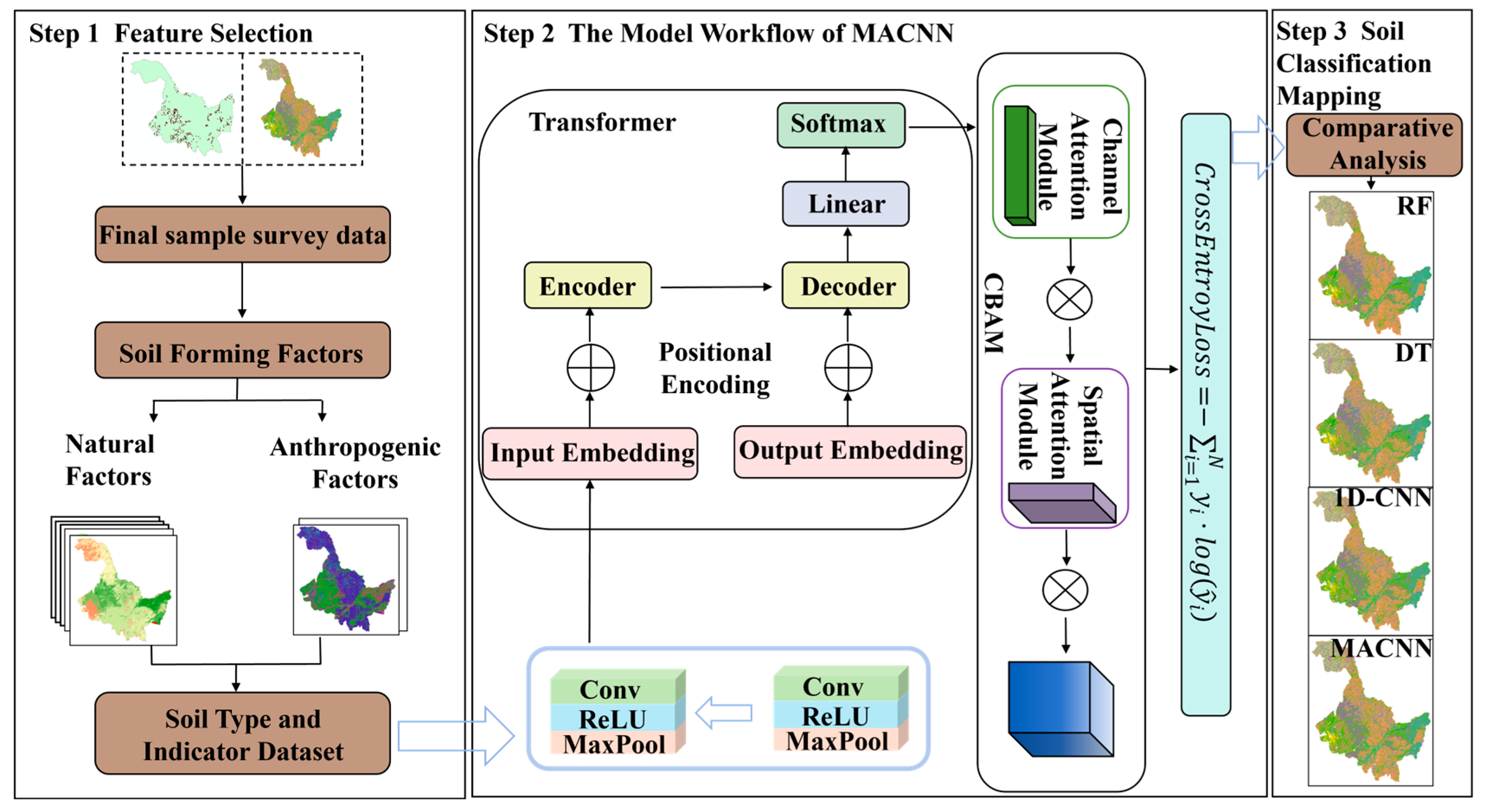
This study proposes a novel MACNN algorithm for digital soil mapping research, with its technical flowchart illustrated in Figure 2. Firstly, representative soil-forming factors, including topography, parent material, climate, and human activities, were selected based on the SCORPAN model. These factors underwent correlation analysis and multicollinearity testing. Subsequently, soil–environment response relationships were established by combining conventional soil map data [30] with field survey data, providing a robust data foundation for algorithm training. Secondly, the MACNN algorithm was constructed. It achieves hierarchical feature extraction through a Convolutional Neural Network (CNN) and incorporates various attention mechanisms for feature enhancement. A cross-entropy loss function was utilized to precisely evaluate the discrepancies between prediction results and true soil types. Finally, taking soil type mapping in Heilongjiang Province as a case study, digital soil mapping was performed using the MACNN algorithm. Its performance was comparatively analyzed against RF, DT, and 1D-CNN algorithms. Furthermore, an ablation experiment assessed the importance of each MACNN module. This systematically validated the algorithm’s reliability and effectiveness for soil type mapping.

2.3.1. Feature Selection

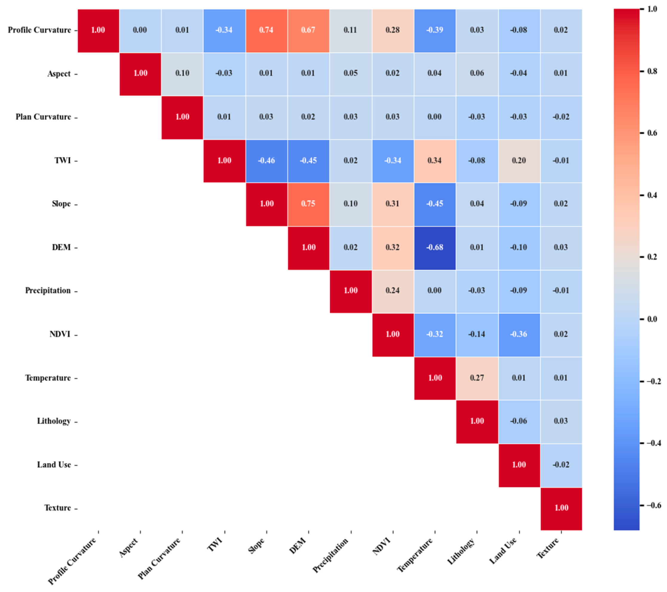
An excessive number of environmental covariate datasets can lead to data redundancy and increased algorithm complexity. This, in turn, may cause overfitting and degrade the algorithm’s generalization capability. Therefore, it is crucial to perform correlation analysis and multicollinearity testing on these environmental covariate datasets. This study first analyzed the correlations among various environmental covariates using Pearson’s correlation coefficient. A Pearson’s correlation coefficient greater than 0.8 typically indicates a high degree of correlation among them. As shown in Figure 3, the Pearson’s correlation coefficients among all selected environmental covariates were found to be less than 0.8, indicating no significant correlation.

To quantify collinearity among environmental covariates, multicollinearity testing was performed using the Variance Inflation Factor (VIF) and Tolerance. A VIF value greater than 5 or a Tolerance value less than 0.2 typically indicates the presence of multicollinearity among the soil-forming factors. As shown in

Table 2. Multicollinearity Analysis Results of Environmental Covariates.

Environmental Covariates	Tolerance	VIF
DEM	0.252	3.969
Slope	0.306	3.266
Profile Curvature	0.411	2.432
Temperature	0.434	2.306
NDVI	0.671	1.490
TWI	0.691	1.448
Lithology	0.827	1.209
Land Use	0.833	1.200
Precipitation	0.907	1.102
Aspect	0.980	1.021
Plan Curvature	0.982	1.018
Texture	0.996	1.004

Note: VIF values exceeding 5 and Tolerance values below 0.20 indicate the presence of significant multicollinearity among the variables.

, all VIF values were less than 5, and all Tolerance values were greater than 0.2. This confirms the absence of significant collinearity among the selected environmental covariates.

2.3.2. MACNN Algorithm

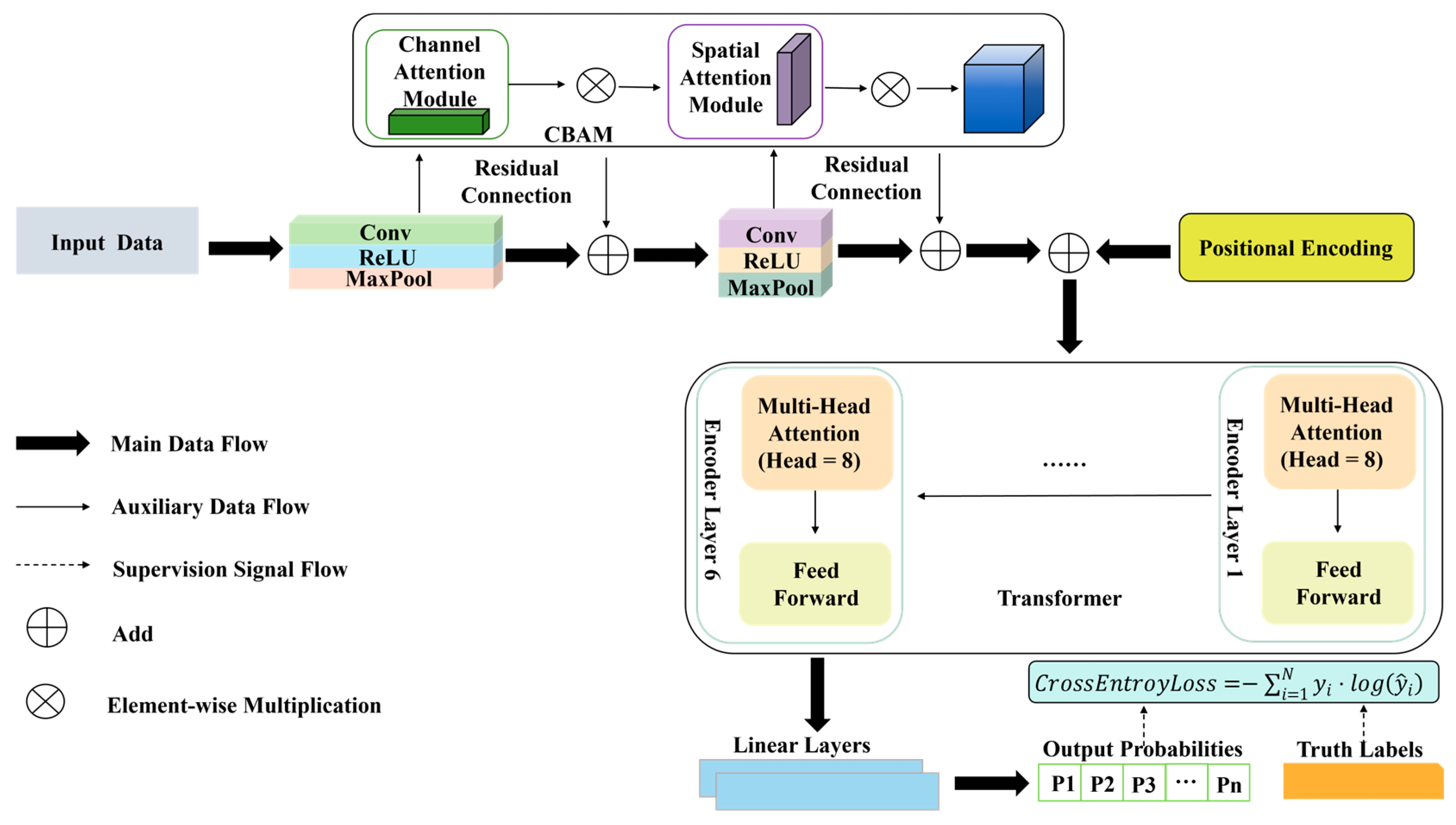
The MACNN algorithm’s core comprises three mutually collaborative functional modules. These modules collectively enable the effective representation and precise classification of soil spatial distribution features. Firstly, hierarchical feature extraction is performed through a CNN. Secondly, Transformer self-attention and multi-head attention mechanisms are integrated to effectively model the long-range dependencies between soil types and features. Concurrently, the Convolutional Block Attention Module (CBAM) is introduced. It features both channel and spatial dual attention mechanisms, enabling adaptive weighting of crucial feature channels and spatial locations. This significantly enhances the algorithm’s sensitivity to discriminative information. Finally, a cross-entropy loss function is employed to evaluate the discrepancies between predicted and true soil types, providing a quantitative basis for parameter optimization. The synergistic action of these three modules allows the MACNN algorithm to overcome the limitations associated with spatial heterogeneity and long-range dependencies (Figure 4).

Hierarchical Convolutional Feature Extraction

The environmental covariate data are fed as input to the CNN [31]. A CNN is a feedforward neural network, characterized by convolutional computations and a deep architecture. It is one of the most important algorithms in deep learning, owing to its powerful feature extraction and automatic representation learning capabilities. A typical CNN structure primarily comprises an input layer, convolutional layers, pooling layers, fully connected layers, and an output layer.

In the convolutional layers, a kernel size of 3 and a stride of 1 were set to capture local relationships between adjacent features and generate corresponding output feature maps. The computationally efficient Rectified Linear Unit (ReLU) was selected as the activation function. Known for introducing non-linearity, ReLU non-linearly maps output feature maps, thereby enhancing the network’s ability to express complex features. Subsequently, max-pooling operations (pool size 2, stride 1) were applied to the feature maps for dimensionality reduction. This reduces computational load while preserving critical information and improving algorithm robustness. Next, the fully connected layers further extract and map features. These layers integrate features from preceding convolutional and pooling layers, learning higher-level representations. Finally, the output layer connects to a SoftMax classifier. This transforms the network’s output into a probability distribution for each soil type, thereby completing the classification task for 19 soil types (Figure 5).

Multi-Attention Mechanism-Based Feature Enhancement

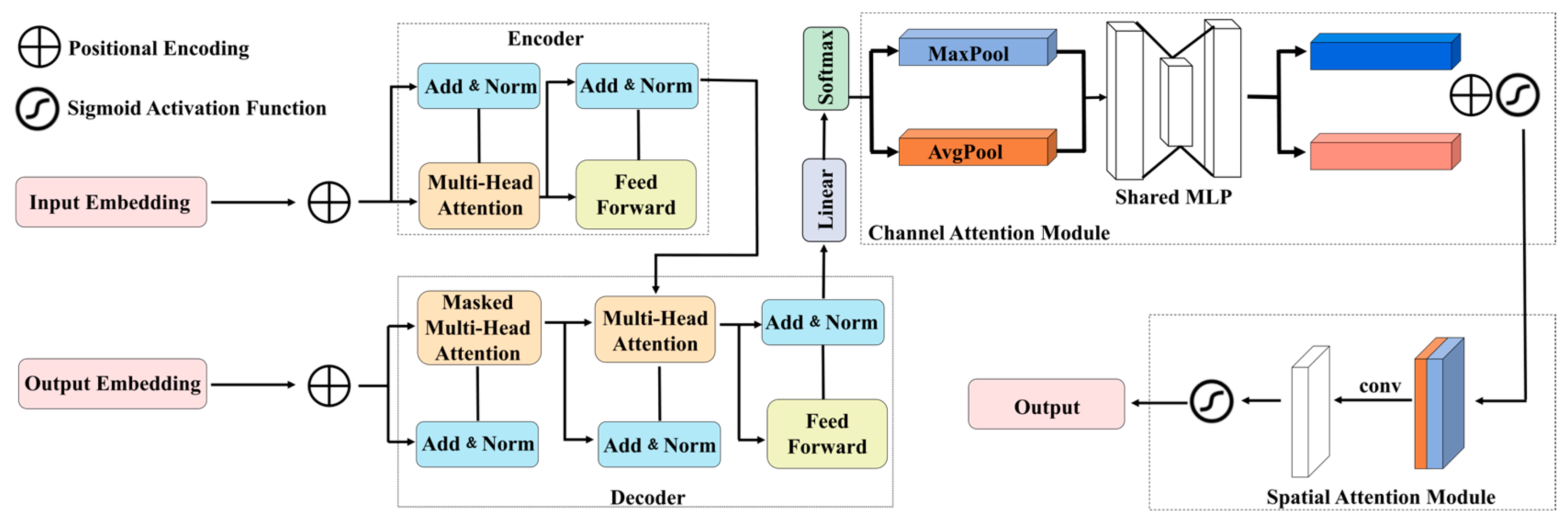
To enhance the algorithm’s discriminative capability for soil types with complex microscopic differences, this study embedded various attention mechanisms into the CNN architecture. This achieved adaptive optimization throughout the entire feature extraction process (Figure 6). Specifically, to address the constraints on local feature extraction caused by CNN’s inherent limited receptive field, this module integrates both self-attention and multi-head attention mechanisms. It models long-range dependencies within the feature sequences, enabling collaborative modeling of local features and global information. Through parallel computation of multi-head self-attention, the algorithm can capture multi-dimensional interactive information between input variables from different subspaces. The algorithm’s ability to model complex soil variations and its global perception of soil classification data are effectively improved. Consequently, this boosts the accuracy and generalization capability of soil type classification.

Within this module, the CBAM [32] is introduced, which comprises a Channel Attention Module and a Spatial Attention Module.

The Channel Attention Module adaptively adjusts the weights of feature channels, enabling the algorithm to focus more on features crucial for the classification task. Specifically, it first aggregates feature information using average pooling and max-pooling operations. Subsequently, the aggregated feature information is fed into a shared Multi-Layer Perceptron (MLP) to generate channel attention weights. Finally, these generated weights are applied to the input feature information, thereby selectively enhancing feature channels that are richer in information.

The Spatial Attention Module optimizes the expression of feature information by focusing on critical spatial regions and suppressing irrelevant or redundant information. Along the channel dimension, it performs average and max pooling, concatenates their results, and then generates a spatial attention map through a convolutional operation. This spatial attention map indicates which spatial regions contain information more crucial for the classification task.

By integrating various attention mechanisms into the CNN architecture, MACNN achieves a holistic perception of both global and local features and enables adaptive feature selection. This allows MACNN to learn more robust feature representations, ultimately leading to an improvement in overall classification accuracy.

Cross-Entropy Loss Function

For multi-class soil type classification tasks, the cross-entropy loss function is employed as an evaluation metric for algorithm optimization. This effectively measures the probabilistic distribution difference between prediction results and true labels, thereby providing a better assessment of the algorithm’s output accuracy. Its formula is presented in Equation (1):

$$\mathrm{CrossEntropyLoss}=-{\sum }_{i=1}^N{y}_i·\mathrm{l}\mathrm{o}\mathrm{g}\left({\hat{y}}_i\right)$$

(1)

In the above formula, $N$ represents the number of categories, $y_i$ represents the true label, and ${\hat{y}}_i$ represents the algorithm’s predicted probability.

2.3.3. Evaluation Metrics

In this study, the accuracy of the classification results was evaluated using four metrics: Overall $Accuracy$ (OA), Producer’s Accuracy (PA), User’s Accuracy (UA), and the Kappa coefficient [33]. OA measures the overall correctness of the algorithm. PA is the fraction of ground-truth samples of a class that are correctly classified. UA represents the probability that a sample classified into a certain category on the map truly belongs to that category. Finally, the Kappa coefficient measures the reliability of the classification, taking into account the possibility of the agreement occurring by chance.

The algorithm’s performance was evaluated using metrics including Accuracy, Precision, Recall, and the Macro-F1 Score. Among these, Accuracy measures the overall proportion of correctly classified samples across all classes. Recall, also known as sensitivity or the true positive rate, is the ratio of correctly identified positive samples to the total number of actual positive samples. Precision is the ratio of correctly identified positive samples to the total number of samples predicted as positive. The Macro-F1 Score is calculated by taking the arithmetic mean of the F1 scores for each individual class. It treats all classes equally, making it a suitable metric for handling imbalanced datasets. The specific formulas for the aforementioned evaluation metrics are as follows:

$$Accuracy={\displaystyle \frac{1}{C}}{\sum }_{i=1}^C{\displaystyle \frac{T{P}_i+T{N}_i}{T{P}_i+T{N}_i+F{P}_i+F{N}_i}}$$

(2)

$$UA={\displaystyle \frac{TP}{TP+FP}}$$

(3)

$$PA={\displaystyle \frac{TP}{TP+FN}}$$

(4)

$$K={\displaystyle \frac{OA-P_e}{1-P_e}}$$

(5)

$$Recall={\displaystyle \frac{1}{C}}{\sum }_{i=1}^C{\displaystyle \frac{T{P}_i}{T{P}_i+F{N}_i}}$$

(6)

$$Precision={\displaystyle \frac{1}{C}}{\sum }_{i=1}^C{\displaystyle \frac{T{P}_i}{T{P}_i+F{P}_i}}$$

(7)

$$MacroF1={\displaystyle \frac{1}{C}}{\sum }_{i=1}^{C}F{1}_i={\displaystyle \frac{1}{C}}{\sum }_{i=1}^{C}2\times {\displaystyle \frac{Precisio{n}_i\times Recal{l}_i}{Precisio{n}_i+Recal{l}_i}}$$

(8)

In the equations above, the terms are defined as follows: $P_e$ represents the probability of the classifier making a correct prediction by random chance.$C$ is the total number of classes. $T{P}_i$ denotes the number of True Positives for class $i$. $T{N}_i$ denotes the number of True Negatives for class $i$. $F{P}_i$ denotes the number of False Positives for class $i$. $F{N}_i$ denotes the number of False Negatives for class $i$. ${Precision}_i$ is the Precision for class $i$. ${Recall}_i$ is the Recall for class $i$. ${F1}_i$ is the F1-score for class $i$.

2.3.4. Parameter Settings

The experiments were conducted on a high-performance server running a Linux operating system, equipped with an NVIDIA GeForce RTX 3090 GPU (24 GB VRAM). The deep learning framework used was PyTorch (V2.7.1), and the scikit-learn (V1.6.1) package was utilized for various utilities.

The dataset was divided into training and test sets at a 9:1 ratio using a stratified random shuffle split method. During the algorithm training phase, the cross-entropy loss function was employed, and the model was iteratively optimized using the AdamW optimizer with an initial learning rate of 1 × 10⁻⁵. To enhance the model’s generalization ability and prevent overfitting, a weight decay of 1 × 10⁻² was applied.

This algorithm employs an 8-head self-attention mechanism, with a feature dimension of 256 and each head having a dimension of 32. Prior to features entering the Transformer encoder, the algorithm integrates a CBAM for weighting. Specifically, channel attention generates weights for each feature channel through global pooling and a Multi-Layer Perceptron (MLP), while spatial attention leverages cross-channel pooling and convolution to generate weights for each spatial location. This sequential process enables focusing on crucial feature channels and spatial positions, respectively.

3. Results Analysis

3.1. Comparison of Soil Type Classification Results

The classification performance of the MACNN algorithm, along with RF, DT, and 1D-CNN algorithms, in mapping 19 soil types in Heilongjiang Province was evaluated using confusion matrices and Kappa coefficients (

Table 3. Comparative Performance of Classification Algorithms for Various Soil Types in Heilongjiang Province.

Soil Type	RF		DT		1D-CNN		MACNN
	UA (%)	PA (%)	UA (%)	PA (%)	UA (%)	PA (%)	UA (%)	PA (%)
Dark-brown earths	83.94	87.65	86.08	81.33	86.71	89.76	88.17	92.16
Albic soils	60.42	72.50	49.39	60.50	71.11	64.00	71.99	73.47
Meadow soils	77.02	59.46	71.25	54.17	68.36	77.44	77.77	78.32
Meadow solonchaks	27.27	60.00	20.00	40.00	28.57	40.00	85.99	89.00
Skeletol soils	50.00	50.00	25.00	50.00	33.33	33.33	78.53	75.00
Aeolian sandy soils	80.00	90.32	57.14	77.42	75.76	80.65	79.00	79.86
Chernozems	56.77	83.87	54.82	80.65	68.39	68.39	77.53	73.53
Black soils	60.34	71,24	62.27	56.86	64.57	65.22	75.36	78.78
Dark felty soils	0.00	0.00	0.00	0.00	100.00	00.00	71.43	62.50
Grey-cinnamon soils	100.00	100.00	100.00	100.00	100.00	100.00	100.00	66.67
Volcanic soils	100.00	60.00	66.67	60.00	83.33	50.00	88.75	78.89
Solonetz	60.00	60.00	33.33	40.00	50.00	40.00	87.56	95.00
Castanozems	100.00	100.00	100.00	100.00	100.00	100.00	52.38	61.11
Peat soils	66.67	60.00	35.71	75.00	100.00	40.00,	77.00	42.78
Litho soils	100.00	33.33	33.33	33.33	100.00	33.33	81.63	74.07
Paddy soils	50.00	60.00	30.51	60.00	81.82	30.00	77.42	62.45
Alluvial soils	41.38	63.16	23.81	52.63	75.00	15.79	55.04	42.26
Bog soils	70.38	57.25	55.12	61.40	76.04	56.74	79.93	69.34
Brown coniferous forest soils	80.49	92.77	75.36	83.53	84.64	90.76	84.87	87.98
OA (%)	73.62		67.76		76.07		81.27
Kappa Coefficient	0.6764		0.6083		0.6996		0.7681

). The results demonstrate that the MACNN algorithm achieved an overall classification accuracy of 81.27%, representing an improvement of 7.65%, 13.51%, and 5.20% over the RF, DT, and 1D-CNN algorithms, respectively. Furthermore, its Kappa coefficient of 0.7681 showed increases of 0.0917, 0.1598, and 0.0685 compared to RF, DT, and 1D-CNN, respectively, indicating significantly higher classification accuracy.

All algorithms demonstrated good classification performance for soil types with higher discriminability based on environmental covariates. For instance, in the classification of Grey-cinnamon soils, MACNN, 1D-CNN, DT, and RF algorithms all achieved a UA of 100%. For the classification of Dark-brown earths, the RF algorithm reached a PA of 87.65%, while the MACNN algorithm also yielded a UA of 88.17% and a PA of 92.16%.

The MACNN algorithm demonstrated a significant advantage in the classification performance of certain soil types. Meadow solonchaks, for instance, represent a typical challenging-to-classify soil type. For this class, the RF algorithm achieved a UA of only 27.27%, exhibiting severe misclassification issues. The DT algorithm suffered from substantial omission and commission errors. In contrast, the MACNN algorithm attained a UA of 85.99% and a PA of 89.00% for this category, achieving both high accuracy and balanced classification performance.

The discrepancies between UA and PA metrics reveal the algorithm’s commission and omission errors. Taking the RF algorithm’s classification of Litho soils as an example, its UA reached an impressive 100.00%, yet its PA was only 33.33%. These figures indicate that while the RF algorithm successfully identified all true Litho soils, it simultaneously misclassified a significant portion of other soil types as Litho soils (commission error). In contrast, the MACNN algorithm achieved a more balanced result for this category, with a UA of 81.63% and a PA of 74.07%. This significantly reduced the omission rate, making the classification results more reliable for practical applications.

Recall, Precision, and Macro-averaged F1-score were employed to quantitatively evaluate the classification performance. In terms of these evaluation metrics, the MACNN algorithm demonstrated significant superiority across all indicators, exhibiting the best overall performance. As shown in

Table 4. Comprehensive Performance Comparison of Different Classification Algorithms.

Algorithm	Recall	Precision	Macro-F1 Score
RF	66.40%	66.56%	64.54%
DT	61.41%	51.57%	54.83%
1D-CNN	61.86%	76.19%	65.42%
MACNN	72.80%	78.44%	75.00%

, the MACNN algorithm achieved a Macro-averaged F1-score of 75.00%, representing an increase of 10.46 percentage points compared to the RF algorithm (64.54%). This score also significantly surpassed those of 1D-CNN (65.42%) and DT (54.83%). The Macro-averaged F1-score effectively and equally reflects the algorithm’s overall classification performance across all classes. This finding fully corroborates that the MACNN algorithm possesses optimal accuracy and robustness when handling complex multi-class soil classification tasks.

3.2. Ablation Study

An ablation study was conducted to assess the importance of the Transformer and CBAM modules within the proposed algorithm. Using the 1D-CNN as the baseline algorithm, different modules were progressively added to analyze the changes in key performance indicators (accuracy, precision, recall, and macro-averaged F1-score) for the soil type classification task. The results are presented in

Table 5. Ablation Study Results: Performance Contributions of MACNN Components for Soil Classification.

1D-CNN	CBAM	Transformer	Accuracy	Recall	Precision	Macro-F1 Score
√			76.07%	61.86%	76.19%	65.42%
√	√		76.80%	65.70%	75.64%	68.38%
√	√	√	81.27%	72.80%	78.44%	75.00%

Note: √ indicates that the module is selected.

. The results indicate that after integrating the CBAM module into the 1D-CNN baseline algorithm, the overall performance of the algorithm improved. Specifically, accuracy, precision, and macro-averaged F1-score showed synchronous growth. This suggests that CBAM effectively guides the algorithm to focus on crucial information, thereby enhancing its robustness. Subsequently, with the further introduction of the Transformer module, performance gains were observed across all evaluation metrics, demonstrating Transformer’s ability to establish long-range dependencies between features.

3.3. Prediction Results

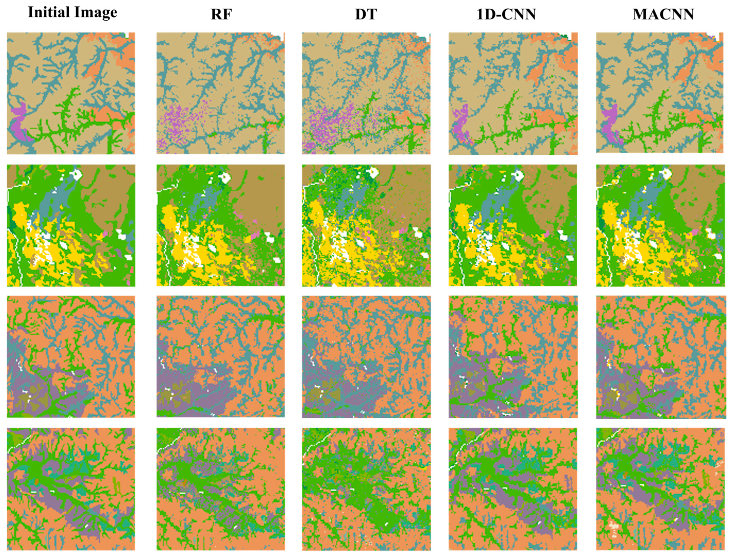
To evaluate the proposed MACNN algorithm’s capability to generate predictive maps for the study area in practical applications, this research conducted digital soil mapping using Heilongjiang Province as a case study. By comparing the performance of RF, DT, 1D-CNN, and MACNN algorithms in digital soil mapping across Heilongjiang Province, distinct differences in accuracy among these algorithms for spatial soil prediction were observed. Figure 7 illustrates the spatial distribution comparison of prediction results from the four algorithms against actual data. For a more in-depth analysis of local feature variations, Figure 8 further provides an enlarged comparative view of typical regions. Analysis results reveal significant differences in the mapping performance among the various algorithms. Specifically, due to its simple structure and susceptibility to overfitting, the DT algorithm exhibited the lowest mapping accuracy. It suffered from both commission and omission errors in soil types with sparse sample points (e.g., Dark felty soils) and showed limited discriminative ability for soil types with similar environmental factors, such as Meadow solonchaks and Solonetz. The RF algorithm enhanced classification stability and accuracy through ensemble learning. However, due to its inherent limitations in sensitivity to high-dimensional sparse features, it exhibited classification bias in local regions, often misclassifying Meadow solonchaks, Dark felty soils, and Solonetz. The 1D-CNN, with its restricted receptive field, struggled to capture long-range dependencies between crucial factors distributed sparsely within the samples. This resulted in suboptimal modeling performance, leading to frequent misclassification and omission errors for the Skeletol soils. In contrast, the MACNN algorithm demonstrated clear advantages. It effectively balanced the mapping performance across different categories, significantly reducing both omission and commission errors. Furthermore, it achieved a substantial improvement in mapping accuracy when dealing with soil types in fragmented areas. Consequently, the soil type map generated by MACNN most closely approximates the true surface conditions, featuring more accurate boundaries and the highest overall reliability.

4. Discussion

4.1. Advantages of the MACNN Algorithm

The MACNN algorithm has demonstrated superior performance compared to existing DSM algorithms. For instance, Zhou et al. [34] utilized the RF algorithm to update original soil maps, achieving a mapping accuracy of 76%. However, its performance is inherently limited by its reliance on pre-extracted, static features and the inability to automatically learn and construct high-level abstract features. Similarly, Beaudoin et al. [35] employed the K-Nearest Neighbor algorithm to generate continuous raster maps of Canadian forest soil attributes. The localized nature of its decision-making process, however, hinders its ability to capture global soil–environment relationships effectively, often leading to the generation of implausible or inconsistent patches in spatial predictions. In contrast, research findings consistently demonstrate that the MACNN algorithm significantly enhances the accuracy of DSM.

The innovation of the MACNN algorithm primarily stems from its sophisticated hierarchical feature extraction capabilities, powered by CNN. Crucially, it integrates the self-attention and multi-head attention mechanisms from Transformers, alongside the channel and spatial attention mechanisms of the CBAM module. This multi-attention approach facilitates a global-local dual optimization of feature information processing, enabling dynamic weight allocation and enhanced responses for features. This sophisticated mechanism effectively mitigates the issue of feature response imbalance often associated with single attention mechanisms, thereby significantly boosting classification accuracy.

4.2. Discussion of Classification and Ablation Experiment Results

From the comparative analysis of classification accuracy between the MACNN algorithm and RF, DT, and 1D-CNN, it is evident that the MACNN algorithm achieves a notable improvement in classification accuracy over the other three methods. This is primarily attributed to its leverage of deep learning’s technical advantages in feature modeling, utilizing the spatial heterogeneity [36] and long-range features of feature vectors for robust representation. However, the current approach overlooks the proximity features among samples. Consequently, there remains room for further improvement. Ablation experiments on module importance showed that integrating both Transformer and CBAM simultaneously into the 1D-CNN baseline yielded the maximum performance gain. However, the contribution of these modules is not a simple linear superposition but rather exhibits significant synergistic gains. The precise mechanism of this synergistic gain remains unclear, warranting further investigation in future studies.

4.3. Limitations of the MACNN Algorithm

The MACNN algorithm presents certain drawbacks in practical applications. Firstly, due to its complex structure integrating multiple attention mechanisms, the algorithm’s computational complexity is higher than that of simpler models. Secondly, when processing sparse soil sample data, particularly for extremely rare soil types, the algorithm tends to learn noise and spurious correlations specific to the training set rather than generalizable soil-forming factor relationships. This can potentially lead to perfect performance on training data but a sharp decline in performance in other regions. Furthermore, the generated soil maps might exhibit spatially overfitted patterns inconsistent with geographical reality.

Future research will consider employing context-aware algorithms to model the true geographical spatial proximity between sample points. Concurrently, introducing Graph Convolutional Neural Networks (GCN) will allow for classification not only based on each soil sample point’s intrinsic features but also by dynamically referencing the features and predicted states of its surrounding neighboring points, thereby generating smoother soil type distribution maps. To ensure the reliability of these soil type distribution maps, spatial autocorrelation analysis, such as Moran’s I, will be incorporated in future work.

5. Conclusions

This study proposes the MACNN algorithm, a deep learning approach that integrates multiple attention mechanisms. It aims to address the limitations of machine learning-based digital soil mapping concerning spatial heterogeneity and long-range dependencies. The MACNN algorithm leverages CNN for hierarchical feature extraction while integrating Transformer’s self-attention and multi-head attention to model long-range dependencies between soil types and features. It also incorporates CBAM’s channel and spatial dual attention for adaptive weighting of crucial feature channels and spatial locations. These combined features significantly enhance the algorithm’s sensitivity to discriminative information. Digital soil mapping for soil type classification was conducted based on the MACNN algorithm, and its accuracy and reliability in this task were systematically evaluated. The main conclusions are as follows:

(1)

A comparative analysis of the classification results of the MACNN algorithm against RF, DT, and 1D-CNN, based on classification accuracy evaluation metrics, was conducted. The results indicate that the MACNN algorithm achieved a substantial improvement in overall classification accuracy. Specifically, MACNN attained an overall classification accuracy of 81.27%, which represents an increase of 7.65%, 13.51%, and 5.20% over the RF, DT, and 1D-CNN algorithms, respectively. Furthermore, its Kappa coefficient of 0.7681 showed respective increases of 0.0917, 0.1598, and 0.0685 compared to RF, DT, and 1D-CNN, thus demonstrating higher classification accuracy and a better ability to represent the spatial distribution of soil types.

(2)

Ablation study results indicate that integrating Transformer and CBAM modules progressively into the 1D-CNN baseline algorithm led to a notable improvement in classification performance, exhibiting a significant synergistic gain effect. Notably, the maximum performance increase was achieved when both Transformer and CBAM were integrated simultaneously. This robustly validates that the proposed MACNN algorithm is both reliable and effective.

(3)

By synergistically combining various attention mechanisms, the MACNN algorithm adaptively focuses on crucial features. This significantly boosts its recognition accuracy for complex soil characteristics. In the visualization of soil type distribution, the model effectively reduces both commission and omission errors, leading to the generation of digital soil type maps with more accurate boundaries and richer details. This algorithm effectively overcomes the limitations in handling spatial heterogeneity and long-range dependencies, thereby offering new technical support for digital soil mapping.

References

1. Liang, A.Z.; Zhang, Y.; Chen, X.W.; Zhang, S.X.; Huang, D.D.; Yang, X.M.; Zhang, X.P.; Li, X.J.; Tian, C.J.; Mclaughlin, N.B.; et al. Development and Effects of Conservation Tillage in the Black Soil Region of Northeast China. Sci. Geogr. Sin. 2022, 42, 1325–1335. [Google Scholar]
2. McKenzie, N.J.; Ryanb, P.J. Spatial prediction of soil properties using environmental correlation. Geoderma 1999, 89, 67–94. [Google Scholar] [CrossRef]
3. Zhu, A.X.; Yang, L.; Fan, N.Q.; Zeng, C.; Zhang, G. The review and outlook of digital soil mapping. Prog. Geogr. 2018, 37, 66–78. [Google Scholar]
4. Hengl, T.; Heuvelink, G.B.M.; Kempen, B.; Leenaars, J.G.B.; Walsh, M.G.; Shepherd, K.D.; Sila, A.; MacMillan, R.A.; de Jesus, J.M.; Tamene, L. Mapping Soil Properties of Africa at 250 m Resolution: Random Forests Significantly Improve Current Predictions. PLoS ONE 2015, 10, e0125814. [Google Scholar] [CrossRef]
5. Chen, R.; Han, H.W.; Fu, P.H.; Yang, Y.; Huang, W. Soil Mapping Based on Multi-temporal Remote Sensing Images and Random Forest Algorithm. Soils 2021, 53, 1087–1094. [Google Scholar]
6. Yang, L.; Sherif, F.; You, J.; Sheldon, H.; Zhu, A.X.; Qin, C.Z.; Xu, Z.G. Updating conventional soil maps using knowledge on soil-environment relationships extracted from the maps. Acta Pedol. Sin. 2010, 47, 1039–1049. [Google Scholar]
7. Guevara, M.; Olmedo, G.F.; Stell, E.; Yigini, Y.; Duarte, Y.A.; Hernández, C.A.; Arévalo, G.E.; Arroyo-Cruz, C.E.; Bolivar, A.; Bunning, S. No silver bullet for digital soil mapping: Country-specific soil organic carbon estimates across Latin America. Soil 2018, 4, 173–193. [Google Scholar] [CrossRef]
8. Lamichhane, S.; Kumar, L.; Wilson, B. Digital soil mapping algorithms and covariates for soil organic carbon mapping and their implications: A review. Geoderma 2019, 352, 395–413. [Google Scholar] [CrossRef]
9. McBratney, A.B.; Odeh, I.O.A.; Bishop, T.F.A.; Dunbar, M.S.; Shatar, T.M. An overview of pedometric techniques for use in soil survey. Geoderma 2000, 97, 293–327. [Google Scholar] [CrossRef]
10. Stoorvogel, J.J.; Bakkenes, M.; Temme, A.J.A.M.; Batjes, N.H.; Brink, B.J.E.T. S-World: A Global Soil Map for Environmental Modelling. Land Degrad. Dev. 2017, 28, 22–33. [Google Scholar] [CrossRef]
11. Mei, S.; Tong, T.; Ying, C.Y.; Wang, T.T.; Zhang, M.; Tang, M.M.; Cai, T.P.; Ma, Y.H.; Wang, Q. Advances in digital soil mapping based on machine learning. J. Agric. Resour. Environ. 2024, 41, 744–756. [Google Scholar]
12. Kovačević, M.; Bajat, B.; Gajić, B. Soil type classification and estimation of soil properties using support vector machines. Geoderma 2010, 154, 340–347. [Google Scholar] [CrossRef]
13. Mansur, N.; Abbod, M. Machine learning-based estimation of soil organic matter using RGB values. Dysona Appl. Sci. 2026, 7, 73–81. [Google Scholar]
14. Song, Q.; Gao, X.; Song, Y.; Li, Q.; Chen, Z.; Li, R.; Zhang, H.; Cai, S. Estimation of soil organic carbon content in farmland based on UAV hyperspectral images: A case study of farmland in the Huangshui River basin. Remote Sens. Nat. Resour. 2024, 36, 160–172. [Google Scholar]
15. Shen, W.; Chen, J.; Zheng, S.; Zhang, L.; Pei, Z.; Lu, W. Deep Learning for Covert Communication. China Commun. 2024, 21, 40–59. [Google Scholar] [CrossRef]
16. Wadoux, A.M.J.-C.; Padarian, J.; Minasny, B. Multi-source data integration for soil mapping using deep learning. Soil 2019, 5, 107–119. [Google Scholar] [CrossRef]
17. Padarian, J.; Minasny, B.; McBratney, A. Using deep learning to predict soil properties from regional spectral data. Geoderma Reg. 2019, 16, e00198. [Google Scholar] [CrossRef]
18. Sun, B.; Hu, W.; Wang, H.; Wang, L.; Deng, C. Remaining Useful Life Prediction of Rolling Bearings Based on CBAM-CNN-LSTM. Sensors 2025, 25, 554. [Google Scholar] [CrossRef]
19. Guo, M.-H.; Xu, T.-X.; Liu, J.-J.; Liu, Z.-N.; Jiang, P.-T.; Mu, T.-J.; Zhang, S.-H.; Martin, R.R.; Cheng, M.-M.; Hu, S.-M. Attention mechanisms in computer vision: A survey. Comput. Vis. Media. 2022, 8, 331–368. [Google Scholar] [CrossRef]
20. McBratney, A.B.; Santos, M.L.M.; Minasny, B. On digital soil mapping. Geoderma 2003, 117, 3–52. [Google Scholar] [CrossRef]
21. Huang, W.; Xu, W.; Wang, S.; Yuan, Y.; Wang, C. Extraction of Knowledge about Soil-environment Relationship Based on an Uncertainty Model. Acta Pedol. Sin. 2018, 55, 54–63. [Google Scholar]
22. Zhang, S.; Zhu, A.; Liu, J.; Yang, L. An Integrative Sampling Scheme for Digital Soil Mapping. Prog. Geogr. 2012, 31, 1318–1325. [Google Scholar]
23. Yang, L.; Zhu, A.; Zhang, S.; An, Y. A comparative study of multi-grade representative sampling and stratified random sampling for soil mapping. Acta Pedol. Sin. 2015, 52, 28–37. [Google Scholar]
24. Xu, B.; Ji, G. A Preliminary Research of Geographic Regionalization of China Land Background and Spectral Reflectance Characteristicsof Soil. J. Remote Sens. 1991, 6, 142–151. [Google Scholar] [CrossRef]
25. Li, L.D.; Chen, J.; Song, X. Application of Spatial Regression Model in Regional Digital Soil Mapping—A Case Study from Fengqiu County, Henan Province. Acta Pedol. Sin. 2013, 50, 21–29. [Google Scholar]
26. Li, W.P.; Zhao, L.; Wu, X.D.; Wang, S.; Nan, Z.T.; Fang, H.B.; Shi, W. Distribution of soils and landform relationships in the permafrost regions of Qinghai-Xizang (Tibetan) Plateau. Chin. Sci. Bull. 2015, 60, 2216–2228. [Google Scholar] [CrossRef]
27. Amundson, R.; Berhe, A.A.; Hopmans, J.W.; Olson, C.; Sztein, A.E.; Sparks, D.L. Soil and human security in the 21st century. Science 2015, 348, 647. [Google Scholar] [CrossRef]
28. Fetene, E.; Amera, M. The effects of land use types and soil depth on soil properties of Agedit watershed, Northwest Ethiopia. Ethiop. J. Sci. Technol. 2018, 11, 39–56. [Google Scholar] [CrossRef]
29. Wang, J.Y.; Liu, F.; Song, X.D.; Cheng, L.D.; Yang, J.L.; Zhang, G.L. Mapping Soil Properties Using the Land Surface Temperature in an Arid Plain. Chin. J. Soil Sci. 2018, 49, 1270–1278. [Google Scholar]
30. Huang, W.; Luo, Y.; Wang, S.Q.; Chen, J.Y.; Han, Z.W.; Qi, D.C. Study on soil-environment relationship acquisition and inference mapping based on traditional soil map. Acta Pedol. Sin. 2016, 53, 72–80. [Google Scholar]
31. Kiranyaz, S.; Avci, O.; Abdeljaber, O.; Ince, T.; Gabbouj, M.; Inman, D.J. 1D convolutional neural networks and applications: A survey. Mech. Syst. Signal Process. 2021, 151, 107398. [Google Scholar] [CrossRef]
32. Woo, S.; Park, J.; Lee, J.Y.; Kweon, I.S. Cbam: Convolutional block attention module. In Proceedings of the European Conference on Computer Vision (ECCV), Munich, Germany, 8–14 September 2018; Volume 11211, pp. 3–19. [Google Scholar]
33. Ye, H.C.; Nie, C.J.; Zhang, Y.; Zhou, Y.; Wang, H.; Huang, Y. Digital Mapping of Soil Types in Different Topographical Units Assisted by Environmental Variables. Trans. Chin. Soc. Agric. 2024, 55, 371–378. [Google Scholar]
34. Zhou, Z.Y.; Huang, W.; Xu, W.; Fu, P.H.; Chen, W.Y. Updating traditional soil maps based on random forest algorithm. J. Huazhong Agric. Univ. 2019, 38, 53–59. [Google Scholar]
35. Beaudoin, A.; Bernier, P.Y.; Guindon, L.; Villemaire, P.; Guo, X.J.; Stinson, G.; Bergeron, T.; Magnussen, S.; Hall, R.J. Mapping attributes of Canada’s forests at moderate resolution through kNN and MODIS imagery. Can. J. For. Res. 2014, 44, 521–532. [Google Scholar] [CrossRef]
36. Zhang, X.T.; Huang, W.; Fu, P.H.; Meng, K.; Wang, S.F. Research on Digital Soil Mapping Based on Feature Selection Algorithm. Acta Pedol. Sin. 2024, 61, 635–647. [Google Scholar]
Figure 1. Study Area Overview and Sample Distribution in Heilongjiang Province. ((a) Geographical location of Heilongjiang Province within China; (b) Heilongjiang’s field and synthetic soil profiles on DEM.).
Agriculture 15 02273 g001
Figure 2. Workflow of Proposed MACNN for Digital Soil Mapping. ((Step 1) Feature Selection. (Step 2) The Model Workflow of MACNN. (Step 3) Soil Classification Mapping.).
Agriculture 15 02273 g002
Figure 3. Pearson’s Correlation Heatmap of Environmental Covariates.
Agriculture 15 02273 g003
Figure 4. MACNN Algorithm Framework.
Agriculture 15 02273 g004
Figure 5. Architecture of the CNN for Hierarchical Feature Extraction and Soil Type Classification.
Agriculture 15 02273 g005
Figure 6. Feature Enhancement Based on Multi-Attention Mechanisms Diagram.
Agriculture 15 02273 g006
Figure 7. Comparative Soil Type Classification Maps of Heilongjiang Province Using Different Algorithms. ((a) Original soil map; (b) Soil type mapping result based on the RF algorithm; (c) Soil type mapping result based on the DT algorithm; (d) Soil type mapping result based on the 1D-CNN algorithm; (e) Soil type mapping result based on the MACNN algorithm; (f) Color representation for each soil type.).
Agriculture 15 02273 g007
Figure 8. Detailed Comparison of Soil Type Classification Maps in Local Areas.
Agriculture 15 02273 g008