
Unsupervised Anomaly Detection with Continuous-Time Model for Pig Farm Environmental Data
 , , ,
, , ,  and
and
Abstract
1. Introduction
- We introduce a novel paradigm of continuous-time neural networks for anomaly detection in pig farming environments. Unlike existing methods, the proposed continuous-time models demonstrate strong ability to capture complex temporal dependencies in multi-sequence multivariate time series data.
- We propose an encoder–decoder architecture based on continuous-time neural networks and adopt an unsupervised learning strategy, enabling end-to-end anomaly detection without the need for labeled data.
- Extensive experiments show that the proposed method consistently outperforms SOTA baseline models in terms of anomaly detection performance, highlighting its robustness and practical applicability in livestock monitoring scenarios.
2. Materials and Methods
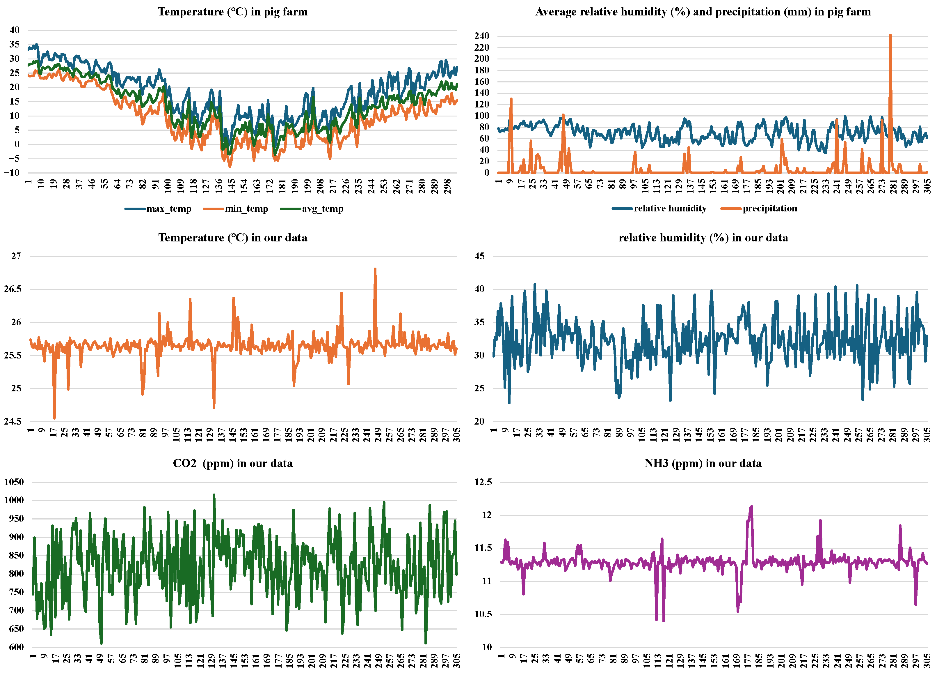
2.1. Dataset
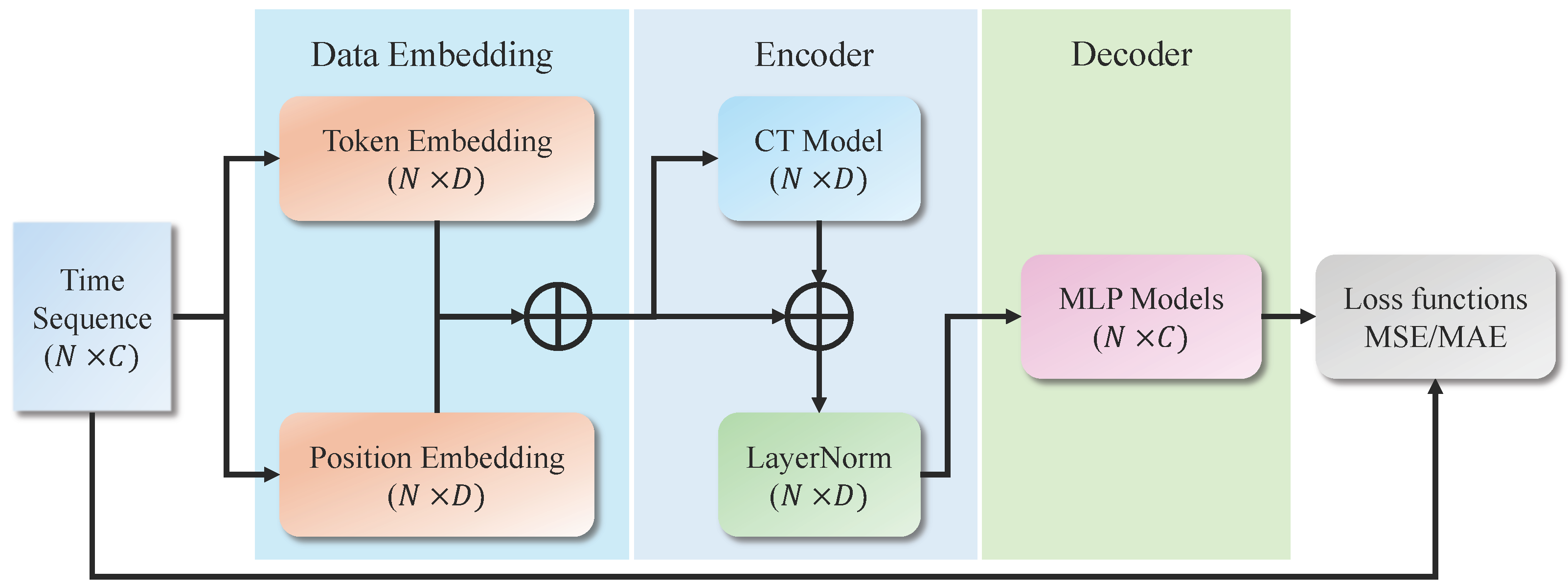
2.2. Methods
2.2.1. Continuous-Time Model
2.2.2. Unsupervised Anomaly Detection
2.2.3. Loss Functions
3. Experiments
3.1. Experimental Setup
3.2. Evaluation Metrics
3.3. Experimental Results
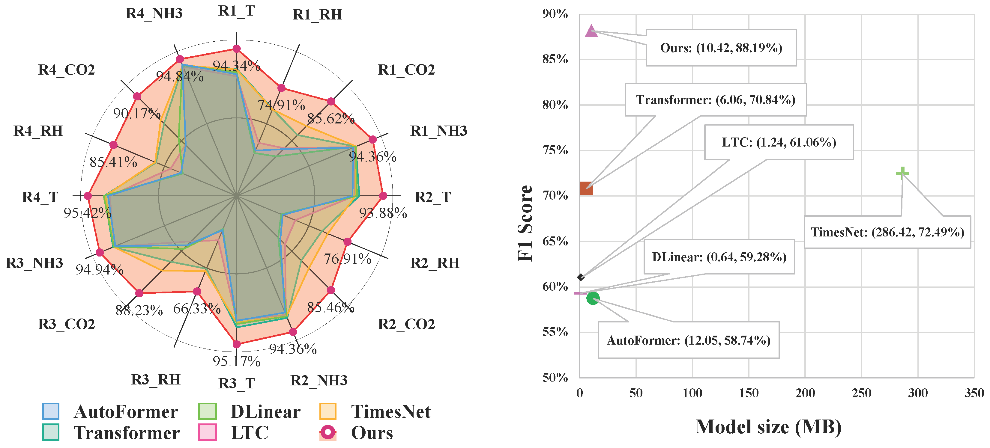
3.3.1. Comparisons with the SOTA Models
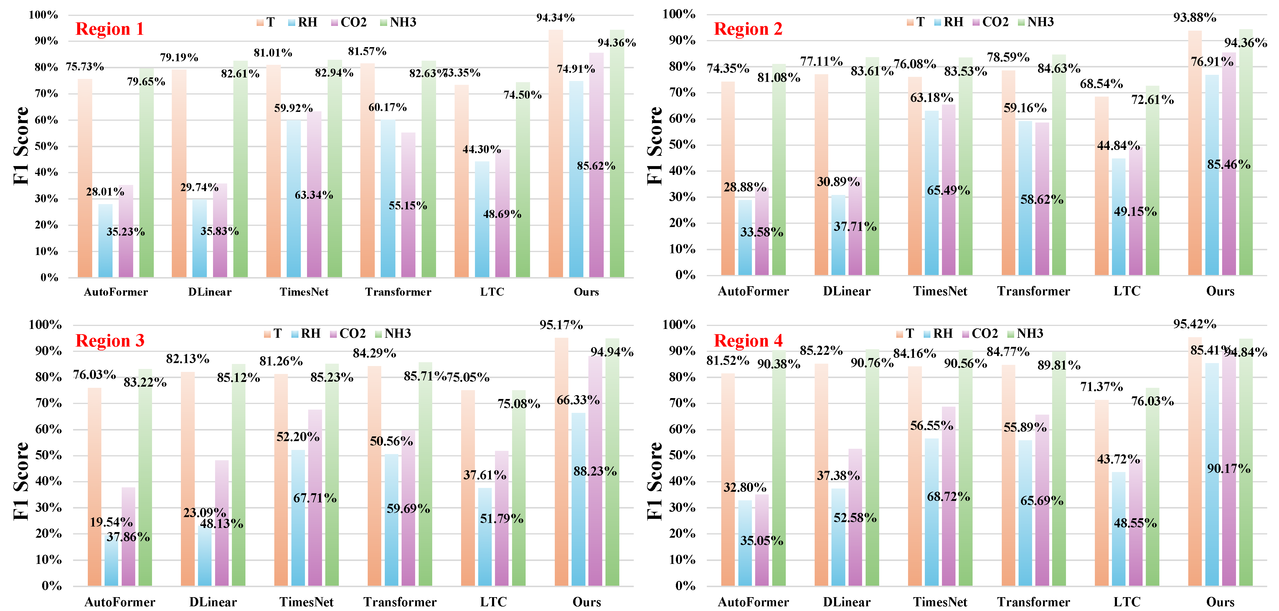
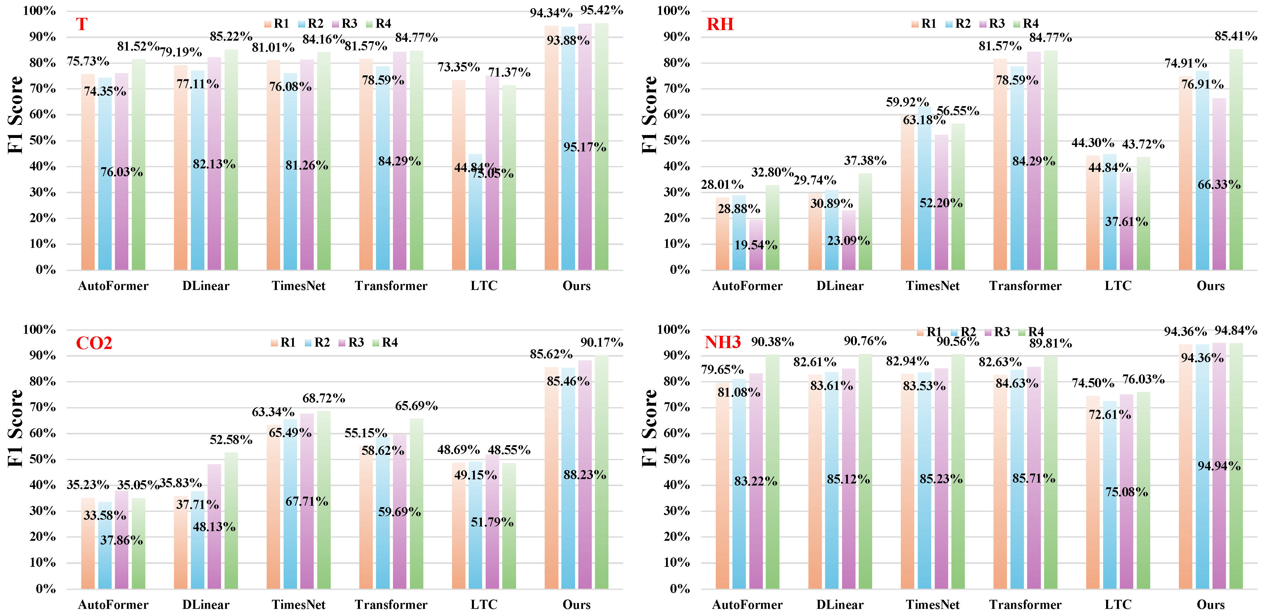
3.3.2. Performance Analysis by Region
3.3.3. Performance Analysis by Variable
3.4. Ablation Studies
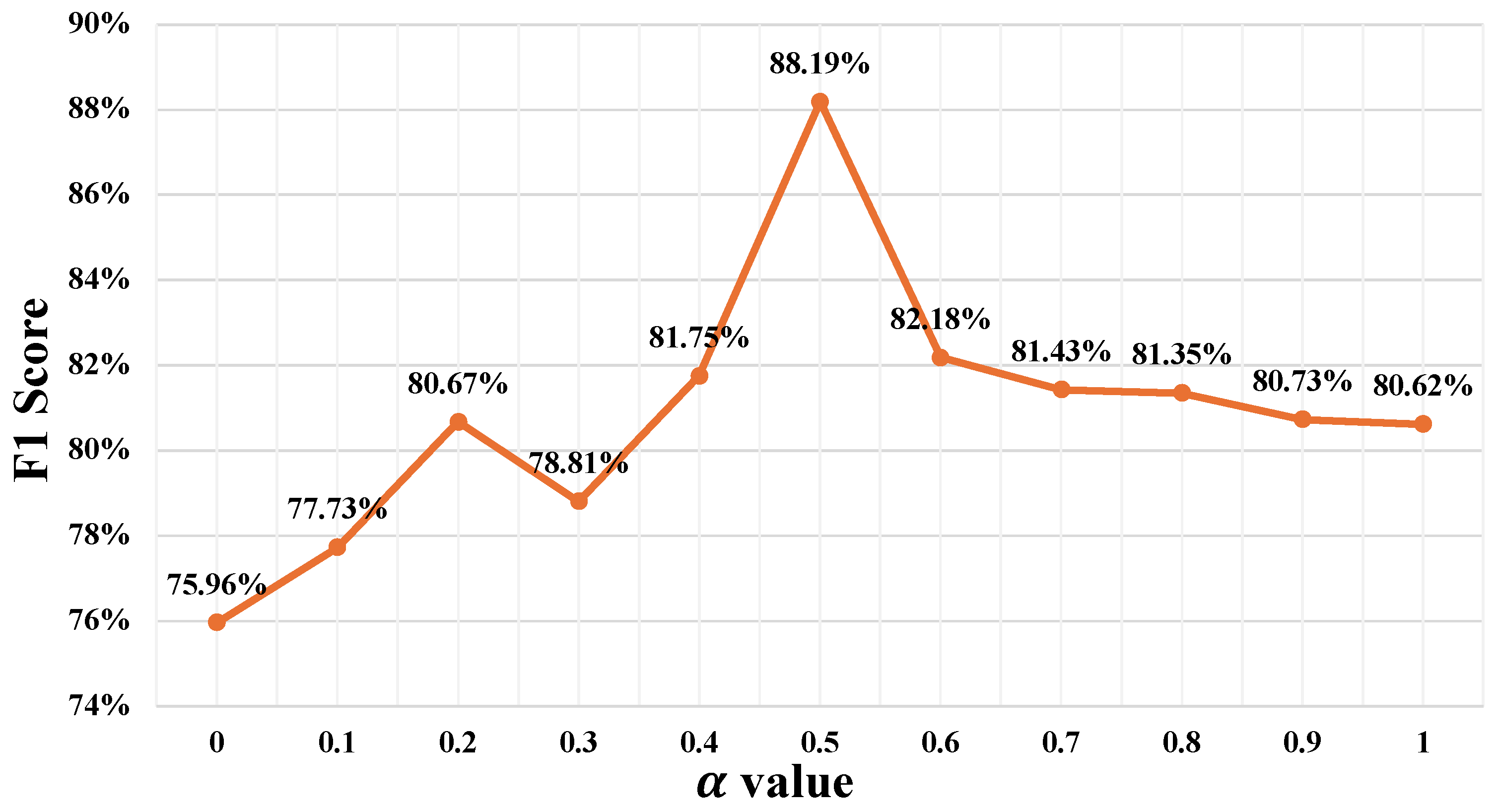
3.4.1. Selection of Loss Functions
3.4.2. Threshold Selection
4. Limitations and Future Work
4.1. Limitations
4.2. Future Work
5. Conclusions
Author Contributions
Funding
Institutional Review Board Statement
Data Availability Statement
Acknowledgments
Conflicts of Interest
Abbreviations
| PLF | Precision Livestock Farming |
| SOTA | State-Of-The-Art |
| T | Temperature |
| RH | Relative Humidity |
| Carbon Dioxide | |
| Ammonia | |
| LSTM | Long Short-Term Memory |
| GRU | Gated Recurrent Units |
| RNN | Recurrent Neural Network |
| TP | True Positive |
| TN | True Negative |
| FP | False Positive |
| RN | False Negative |
References
- Kleen, J.L.; Guatteo, R. Precision Livestock Farming: What Does It Contain and What Are the Perspectives? Animals 2023, 13, 779. [Google Scholar] [CrossRef] [PubMed]
- Tullo, E.; Finzi, A.; Guarino, M. Review: Environmental impact of livestock farming and Precision Livestock Farming as a mitigation strategy. Sci. Total Environ. 2019, 650, 2751–2760. [Google Scholar] [CrossRef] [PubMed]
- Williams, L.R.; Moore, S.T.; Bishop-Hurley, G.J.; Swain, D.L. A sensor-based solution to monitor grazing cattle drinking behaviour and water intake. Comput. Electron. Agric. 2020, 168, 105141. [Google Scholar] [CrossRef]
- Biszkup, M.; Vásárhelyi, G.; Setiawan, N.N.; Márton, A.; Szentes, S.; Balogh, P.; Babay-Török, B.; Pajor, G.; Drexler, D. Detectability of multi-dimensional movement and behaviour in cattle using sensor data and machine learning algorithms: Study on a Charolais bull. Artif. Intell. Agric. 2024, 14, 86–98. [Google Scholar] [CrossRef]
- Ma, S.; Yao, Q.; Masuda, T.; Higaki, S.; Yoshioka, K.; Arai, S.; Takamatsu, S.; Itoh, T. Development of Noncontact Body Temperature Monitoring and Prediction System for Livestock Cattle. IEEE Sens. J. 2021, 21, 9367–9376. [Google Scholar] [CrossRef]
- Rebez, E.B.; Sejian, V.; Silpa, M.V.; Kalaignazhal, G.; Thirunavukkarasu, D.; Devaraj, C.; Nikhil, K.T.; Ninan, J.; Sahoo, A.; Lacetera, N.; et al. Applications of Artificial Intelligence for Heat Stress Management in Ruminant Livestock. Sensors 2024, 24, 5890. [Google Scholar] [CrossRef]
- Provolo, G.; Brandolese, C.; Grotto, M.; Marinucci, A.; Fossati, N.; Ferrari, O.; Beretta, E.; Riva, E. An Internet of Things Framework for Monitoring Environmental Conditions in Livestock Housing to Improve Animal Welfare and Assess Environmental Impact. Animals 2025, 15, 644. [Google Scholar] [CrossRef]
- Džermeikaitė, K.; Bačėninaitė, D.; Antanaitis, R. Innovations in Cattle Farming: Application of Innovative Technologies and Sensors in the Diagnosis of Diseases. Animals 2023, 13, 780. [Google Scholar] [CrossRef]
- Han, C.S.; Kaur, U.; Bai, H.; Roqueto dos Reis, B.; White, R.; Nawrocki, R.A.; Voyles, R.M.; Kang, M.G.; Priya, S. Invited review: Sensor technologies for real-time monitoring of the rumen environment. J. Dairy Sci. 2022, 105, 6379–6404. [Google Scholar] [CrossRef]
- Post, C.; Rietz, C.; Büscher, W.; Müller, U. The Importance of Low Daily Risk for the Prediction of Treatment Events of Individual Dairy Cows with Sensor Systems. Sensors 2021, 21, 1389. [Google Scholar] [CrossRef]
- Benjamin, M.; Yik, S. Precision Livestock Farming in Swine Welfare: A Review for Swine Practitioners. Animals 2019, 9, 133. [Google Scholar] [CrossRef] [PubMed]
- Neethirajan, S. Artificial Intelligence and Sensor Innovations: Enhancing Livestock Welfare with a Human-Centric Approach. Hum. Centric Intell. Syst. 2024, 4, 77–92. [Google Scholar] [CrossRef]
- Zhou, H.; Chung, S.; Kakar, J.K.; Kim, S.C.; Kim, H. Pig movement estimation by integrating optical flow with a multi-object tracking model. Sensors 2023, 23, 9499. [Google Scholar] [CrossRef] [PubMed]
- Zhou, H.; Dong, J.; Han, S.; Chung, S.; Ali, H.; Kim, S. Weakly supervised learning through box annotations for pig instance segmentation. Sci. Rep. 2025, 15, 19706. [Google Scholar] [CrossRef]
- Louie, A.; Rowe, J.; Love, W.; Lehenbauer, T.; Aly, S. Effect of the environment on the risk of respiratory disease in preweaning dairy calves during summer months. J. Dairy Sci. 2018, 101, 10230–10247. [Google Scholar] [CrossRef]
- Koknaroglu, H.; Otles, Z.; Mader, T.; Hoffman, M.P. Environmental factors affecting feed intake of steers in different housing systems in the summer. Int. J. Biometeorol. 2008, 52, 419–429. [Google Scholar] [CrossRef]
- Pompeo, J.; Yu, Z.; Zhang, C.; Wu, S.; Zhang, Y.; Gomez, C.; Correll, M. Assessing the stability of indoor farming systems using data outlier detection. Front. Plant Sci. 2025, 15, 1270544. [Google Scholar] [CrossRef]
- Jung, J.M.; Kim, D.H.; Cho, H.; Lee, M.; Jeong, J.; Lee, D.H.; Seo, S.; Lee, W.H. Multi-algorithmic approach for detecting outliers in cattle intake data. J. Agric. Food Res. 2024, 15, 101021. [Google Scholar] [CrossRef]
- Suryavansh, S.; Benna, A.; Guest, C.; Chaterji, S. A data-driven approach to increasing the lifetime of IoT sensor nodes. Sci. Rep. 2021, 11, 22459. [Google Scholar] [CrossRef]
- Ou, C.H.; Chen, Y.A.; Huang, T.W.; Huang, N.F. Design and Implementation of Anomaly Condition Detection in Agricultural IoT Platform System. In Proceedings of the 2020 International Conference on Information Networking (ICOIN), Barcelona, Spain, 7–10 January 2020; pp. 184–189. [Google Scholar] [CrossRef]
- Wu, H.; Xu, J.; Wang, J.; Long, M. Autoformer: Decomposition transformers with auto-correlation for long-term series forecasting. Adv. Neural Inf. Process. Syst. 2021, 34, 22419–22430. [Google Scholar]
- Wu, H.; Hu, T.; Liu, Y.; Zhou, H.; Wang, J.; Long, M. TimesNet: Temporal 2D-Variation Modeling for General Time Series Analysis. In Proceedings of the International Conference on Learning Representations, Kigali, Rwanda, 1–5 May 2023. [Google Scholar]
- Zeng, A.; Chen, M.; Zhang, L.; Xu, Q. Are transformers effective for time series forecasting? Proc. AAAI Conf. Artif. Intell. 2023, 37, 11121–11128. [Google Scholar] [CrossRef]
- Guo, Z.; Yin, Z.; Lyu, Y.; Wang, Y.; Chen, S.; Li, Y.; Zhang, W.; Gao, P. Research on indoor environment prediction of pig house based on OTDBO–TCN–GRU algorithm. Animals 2024, 14, 863. [Google Scholar] [CrossRef] [PubMed]
- Rong, L.; Fan, J.; Guo, X.; Tong, Z.; Xu, W.; Pan, Y.; Li, S.; Zhang, W.; Sun, F. Reserach on environmental monitoring and comprehensive evaluation system of pig house based on internet of things technology. INMATEH Agric. Eng. 2025, 75, 501. [Google Scholar] [CrossRef]
- Park, H.; Park, D.; Kim, S. Anomaly detection of operating equipment in livestock farms using deep learning techniques. Electronics 2021, 10, 1958. [Google Scholar] [CrossRef]
- Peng, S.; Zhu, J.; Liu, Z.; Hu, B.; Wang, M.; Pu, S. Prediction of ammonia concentration in a pig house based on machine learning models and environmental parameters. Animals 2022, 13, 165. [Google Scholar] [CrossRef]
- Jin, H.; Meng, G.; Pan, Y.; Zhang, X.; Wang, C. An improved intelligent control system for temperature and humidity in a pig house. Agriculture 2022, 12, 1987. [Google Scholar] [CrossRef]
- Li, H.; Li, H.; Li, B.; Shao, J.; Song, Y.; Liu, Z. Smart temperature and humidity control in pig house by improved three-way K-means. Agriculture 2023, 13, 2020. [Google Scholar] [CrossRef]
- Chen, R.T.Q.; Rubanova, Y.; Bettencourt, J.; Duvenaud, D.K. Neural Ordinary Differential Equations. In Advances in Neural Information Processing Systems; Bengio, S., Wallach, H., Larochelle, H., Grauman, K., Cesa-Bianchi, N., Garnett, R., Eds.; Curran Associates, Inc.: Red Hook, NY, USA, 2018; Volume 31. [Google Scholar]
- Baytas, I.M.; Xiao, C.; Zhang, X.; Wang, F.; Jain, A.K.; Zhou, J. Patient subtyping via time-aware LSTM networks. In Proceedings of the 23rd ACM SIGKDD International Conference on Knowledge Discovery and Data Mining, Montréal, QC, Canada, 2–8 December 2018; pp. 65–74. [Google Scholar]
- Hasani, R.; Lechner, M.; Amini, A.; Rus, D.; Grosu, R. Liquid time-constant networks. Proc. AAAI Conf. Artif. Intell. 2021, 35, 7657–7666. [Google Scholar] [CrossRef]
- Hasani, R.; Lechner, M.; Amini, A.; Liebenwein, L.; Ray, A.; Tschaikowski, M.; Teschl, G.; Rus, D. Closed-form continuous-time neural networks. Nat. Mach. Intell. 2022, 4, 992–1003. [Google Scholar] [CrossRef]
- Vaswani, A.; Shazeer, N.; Parmar, N.; Uszkoreit, J.; Jones, L.; Gomez, A.N.; Kaiser, Ł; Polosukhin, I. Attention is all you need. arXiv 2017, arXiv:1706.03762. [Google Scholar]

| Region ID | Training | Validation | Testing |
|---|---|---|---|
| 1 | 19,008 | 6336 | 6336 |
| 2 | 18,144 | 6048 | 6336 |
| 3 | 7488 | 2304 | 2880 |
| 4 | 7776 | 2592 | 2592 |
| Total | 52,416 | 17,280 | 18,144 |
| Models | Accuracy | Precision | Recall | F1 Score | |
|---|---|---|---|---|---|
| AutoFormer [21] | T | 68.22% | 68.32% | 90.06% | 77.70% |
| RH | 56.98% | 23.94% | 47.04% | 31.73% | |
| 56.99% | 35.50% | 52.79% | 42.45% | ||
| 74.18% | 74.63 | 93.71% | 83.09% | ||
| Average | 64.09% | 50.59% | 70.90% | 58.74% | |
| DLinear [23] | T | 73.30% | 74.30% | 86.50% | 79.93% |
| RH | 74.45% | 36.27% | 26.69% | 30.75% | |
| 67.23% | 44.81% | 39.07% | 41.74% | ||
| 77.33% | 77.99% | 92.64% | 84.68% | ||
| Average | 73.08% | 58.34% | 61.22% | 59.28% | |
| TimesNet [22] | T | 73.77% | 75.42% | 85.04% | 79.94% |
| RH | 85.12% | 70.54% | 51.48% | 59.52% | |
| 79.98% | 67.70% | 63.83% | 65.71% | ||
| 78.34% | 80.72% | 89.32% | 84.80% | ||
| Average | 79.30% | 73.60% | 72.42% | 72.49% | |
| Transformer [34] | T | 75.60% | 76.23% | 87.65% | 81.54% |
| RH | 84.55% | 68.83% | 49.87% | 57.83% | |
| 77.24% | 64.29% | 54.55% | 59.02% | ||
| 78.27% | 79.85% | 90.80% | 84.97% | ||
| Average | 78.91% | 72.30% | 70.72% | 70.84% | |
| LTC [32] | T | 70.66% | 73.35% | 82.09% | 77.48% |
| RH | 75.56% | 41.56% | 36.93% | 39.11% | |
| 69.11% | 48.30% | 39.75% | 43.61% | ||
| 76.46% | 78.22% | 90.38% | 83.86% | ||
| Average | 72.95% | 60.36% | 62.29% | 61.60% | |
| Ours | T | 93.09% | 92.61% | 96.46% | 94.50% |
| RH | 91.50% | 91.32% | 66.31% | 76.83% | |
| 92.55% | 92.13% | 82.23% | 86.90% | ||
| 92.42% | 92.25% | 96.94% | 94.53% | ||
| Average | 92.39% | 92.08% | 85.84% | 88.19% |
| Threshold | F1 Score | |
|---|---|---|
| Separate Values | [0.49, 0.17, 0.20, 0.53] | 88.19% |
| Unified Values | 0.1 | 62.93% |
| 0.17 | 77.38% | |
| 0.2 | 79.99% | |
| 0.3 | 79.46% | |
| 0.4 | 77.59% | |
| 0.49 | 76.05% | |
| 0.5 | 75.67% | |
| 0.53 | 74.66% | |
Disclaimer/Publisher’s Note: The statements, opinions and data contained in all publications are solely those of the individual author(s) and contributor(s) and not of MDPI and/or the editor(s). MDPI and/or the editor(s) disclaim responsibility for any injury to people or property resulting from any ideas, methods, instructions or products referred to in the content. |
© 2025 by the authors. Licensee MDPI, Basel, Switzerland. This article is an open access article distributed under the terms and conditions of the Creative Commons Attribution (CC BY) license (https://creativecommons.org/licenses/by/4.0/).
Share and Cite
Zhou, H.; Chung, S.; Waqar, M.M.; Zain Ul Abideen, M.I.; Ahmad, A.; Ilyas, M.A.; Kim, H.; Kim, S. Unsupervised Anomaly Detection with Continuous-Time Model for Pig Farm Environmental Data. Agriculture 2025, 15, 1419. https://doi.org/10.3390/agriculture15131419
Zhou H, Chung S, Waqar MM, Zain Ul Abideen MI, Ahmad A, Ilyas MA, Kim H, Kim S. Unsupervised Anomaly Detection with Continuous-Time Model for Pig Farm Environmental Data. Agriculture. 2025; 15(13):1419. https://doi.org/10.3390/agriculture15131419
Chicago/Turabian StyleZhou, Heng, Seyeon Chung, Malik Muhammad Waqar, Muhammad Ibrahim Zain Ul Abideen, Arsalan Ahmad, Muhammad Ans Ilyas, Hyongsuk Kim, and Sangcheol Kim. 2025. "Unsupervised Anomaly Detection with Continuous-Time Model for Pig Farm Environmental Data" Agriculture 15, no. 13: 1419. https://doi.org/10.3390/agriculture15131419
APA StyleZhou, H., Chung, S., Waqar, M. M., Zain Ul Abideen, M. I., Ahmad, A., Ilyas, M. A., Kim, H., & Kim, S. (2025). Unsupervised Anomaly Detection with Continuous-Time Model for Pig Farm Environmental Data. Agriculture, 15(13), 1419. https://doi.org/10.3390/agriculture15131419