A Two-Stage Machine Learning Approach for Calving Detection in Rangeland Cattle

Abstract

Monitoring parturient cattle during calving is crucial for reducing cow and calf mortality, enhancing reproductive and production performance, and minimizing labor costs. Traditional monitoring methods include direct animal inspection or the use of specialized sensors. These methods can be effective, but impractical in large-scale ranching operations due to time, cost, and logistical constraints. To address this challenge, a network of low-power and long-range IoT sensors combining the Global Navigation Satellite System (GNSS) and tri-axial accelerometers was deployed to monitor in real-time 15 parturient Brangus cows on a 700-hectare pasture at the Chihuahuan Desert Rangeland Research Center (CDRRC). A two-stage machine learning approach was tested. In the first stage, a fully connected autoencoder with time encoding was used for unsupervised detection of anomalous behavior. In the second stage, a Random Forest classifier was applied to distinguish calving events from other detected anomalies. A 5-fold cross-validation, using 12 cows for training and 3 cows for testing, was applied at each iteration. While 100% of the calving events were successfully detected by the autoencoder, the Random Forest model failed to classify the calving events of two cows and misidentified the onset of calving for a third cow by 46 h. The proposed framework demonstrates the value of combining unsupervised and supervised machine learning techniques for detecting calving events in rangeland cattle under extensive management conditions. The real-time application of the proposed AI-driven monitoring system has the potential to enhance animal welfare and productivity, improve operational efficiency, and reduce labor demands in large-scale ranching. Future advancements in multi-sensor platforms and model refinements could further boost detection accuracy, making this approach increasingly adaptable across diverse management systems, herd structures, and environmental conditions.

1. Introduction

Precision ranching leverages advanced technologies such as smart sensors, Global Navigation Satellite System (GNSS) tracking, and data analytics to monitor and manage livestock and rangeland resources more efficiently. It enables ranchers to make informed decisions that can improve productivity, animal welfare, and environmental sustainability.

Traditionally, precision livestock management has been associated with intensive animal production systems such as dairy cattle and sheep farming and hog and poultry production [1]. However, with advances in sensor technology, the availability of long-range wireless transmission networks, and new analytic tools, there has been a growing interest in expanding similar concepts to large-scale beef production systems and cattle ranching. Precision ranching applications are becoming increasingly widespread, accessible, and affordable, enabling data-driven decision-making in real time [1].

In cattle production systems operating on extensive rangelands, parturition or calving is a critical event in the life cycle of cows with significant implications for animal productivity, health, and welfare. Efficient monitoring of cows around calving is therefore essential to reduce losses associated with cow and calf mortality, and to minimize the labor costs required to inspect animals regularly. Furthermore, dystocia can negatively impair the health of cows and calves, underscoring the need for timely detection and intervention [2]. Also, risks around calving due to adverse weather conditions and predation can be mitigated when cows and calves are monitored regularly before, during, and after calving [3]. However, the regular inspection of cattle is not feasible in large-scale ranch operations, where ranchers must travel long distances across difficult terrain or woodlands to find animals. These challenges underscore the need to develop accurate and reliable calving monitoring systems tailored to the unique challenges of extensive cattle ranches operating on remote rangelands.

Various methods have been developed to monitor parturient dairy and beef cows to detect calving [4]. A common approach is the use of devices to monitor behavioral and physiological parameters associated with calving. Ricci et al. [5] evaluated intravaginal devices expelled at calving to alert calving based on differences between body temperature and environmental temperature. The use of intravaginal devices were reliable for calving detection, with a reported predictive value of 100% [6]. Schirmann et al. [7] used microphones mounted to a cattle neck collar to monitor rumination and feeding time of dairy cows in the hours before calving. Compared to baseline values, rumination time decreased by an average of 63 ± 30 min whereas feeding time decreases by an average of 66 ± 16 min within the 24 h preceding calving. Chang et al. [8] used a walk-over-weighing scale placed near the water source to alert sudden changes in body weight associated with calving. Tail inclinometers and accelerometers were also tested for the early detection of calving [9]. Yang et al. [10] applied deep learning modeling on triaxial and x-axis tail acceleration data to detect calving of dairy cows within 12 h with a success rate of 91%. Similarly, Miller et al. [11] applied a Random Forest classifier both on tail- and neck-mounted accelerometers and found a significant correlation between the time of a dairy or beef calf birth and the accelerometer data. Liseune et al. [12] proposed a two-stage deep learning model combining CNNs and LSTMs applied to neck and leg acceleration and found that 65% of calving events of dairy cows in a 24 h window were detected with a precision of 77%. Finally, computer vision applied to video was investigated with different degrees of success and feasibility for deployment on commercial farms. Sumi et al. [13] proposed a method for the automatic detection of calving integrating depth cameras, image processing, computer vision, and coordinate transformation concepts. Hyodo et al. [14] designed neural networks to extract calving-related information such as the frequency of postures, movement, and rotational statistics. Recently, Mg et al. [15] trained a tailored YOLOv8 model to track 360-degree videos showing changes in the posture, trajectory, and movement of dairy cows in a common pen and reported 100%, 95%, and 85% accuracy in classifying abnormal or normal calving and predicted calving time within 6 h, 8 h, and 9 h, respectively. Despite the method demonstrating promise, it was applied to monitor a few cows in a controlled setting, suggesting limited opportunities for commercial deployment on a large pasture setting.

The accurate detection of calving in a cattle ranching operation presents a unique set of challenges [16]. Sensor durability, battery life, passive data transmission, and ease of deployment may limit the application of sensor-based techniques on rangelands. Many operating sensors have high power demands, limiting their operational lifetime when relying solely on batteries. Devices such as video cameras can be further constrained by installation requirements. For example, placing multiple cameras to capture regular images of cattle may not be feasible due to limited infrastructure, lacking connectivity, and limited power supply. Moreover, in a large rangeland pasture, camera functionality can be severely restricted by a narrow field of view, further limiting their effectiveness in large, open rangelands.

This study aims to address key technological and knowledge gaps to monitor the calving of beef cattle in large pastures of open rangeland. We applied low-power GNSS and accelerometer sensors embedded in cattle tracking collars coupled with long-range data transmission networks streaming sensor data in real-time. This approach was designed to maximize sensor battery life and ensure system stability. The analytical method integrated both unsupervised (an autoencoder) and supervised (a Random Forest classifier) learning approaches to detect calving events of cows managed on rangeland pasture.

2. Materials and Methods

Field trials were conducted at the Chihuahuan Desert Rangeland Research Center (CDRRC) of New Mexico State University (NMSU), between January and May of 2023. The CDRRC (32.529° N, −106.804° W) is located approximately 30 miles north of Las Cruces, New Mexico. All animal handling and monitoring protocols followed guidelines reviewed and approved by NMSU’s IACUC (protocol 3159-001).

2.1. Study Site

The CDRRC spans approximately 64,000 acres across the Jornada del Muerto Basin at the northern edge of the Chihuahuan Desert ecoregion. The terrain is predominantly flat, with an average elevation of 4000 feet [17]. The climate is characteristic of hot desert regions. The average annual precipitation is 247 mm, with more than half typically falling between July and September. Mean ambient temperatures peak in June at approximately 36.0 °C and reach their lowest in January, averaging around 13.3 °C. The vegetation at the CDRRC is dominated by honey mesquite (Prosopis glandulosa Torr.) interspersed with native grasses, including black grama (Bouteloua eriopoda), dropseeds (Sporobolus spp.), and threeawns (Aristida spp.). The CDRRC has a rich and diverse wildlife population. Mountain lions, coyotes, oryx, and mule deer are sighted regularly at the site [17]. Figure 1 depicts the landscape and typical shrubland and grassland plant communities at CDRRC.

The CDRRC is subdivided into multiple pastures for rotational grazing of livestock [17]. During this study the cattle were managed at pasture 3 west (abbreviated as 3w) which is located at the north end of the ranch and consist of 700 ha of flat terrain covered predominantly by desert grassland vegetation. Figure 2 shows the map of the CDRRC, pasture 3w, and the cattle used in this study.

2.2. Cattle Management and Monitoring

Fifteen multiparous Brangus cows, aged between four and eight years, were used in this study. These cows were born and raised at the CDRRC and were therefore well-adapted to the harsh climatic and nutritional conditions typical of Northern Chihuahuan Desert rangelands. The reproduction management of cows was as follows. Fixed-Time Artificial Insemination (FTAI) was performed on all cows after a forty-day postpartum waiting period. This was followed by a ninety-day natural breeding with bulls. Pregnancy diagnosis via rectal palpation was conducted ninety days after the bulls were removed. By knowing the start and end dates of the breeding season and pregnancy tests, the expected calving season was projected using a standard gestation length of 282 days. For the 2022 breeding season, FTAI was initiated on 11 May. Consequently, the monitoring of calving took place approximately between 17 February and 18 May 2023. All cows were in the late gestation stage at study onset.

Two months prior to the beginning of the monitoring phase, cows were fitted with Compact Trackers 2.1.1 (CT; Abeeway, Biot, France) mounted on a neck collar (Figure 2b). The collar was made of a 40 mm-wide nylon strap and included a flat aluminum bracket covered by a rubber tube to secure the CT devices. A 500 g counterweight was added to the collar to keep the CTs in an upright position, ensuring consistent orientation to optimize data gathering and transmission capabilities. The CTs are relatively small devices (11 × 6 × 2.5 cm) equipped with a GNSS receptor, temperature sensor, triaxial accelerometer, and LoRaWAN antenna. The CTs were used to monitor both the positions and movements of cows during this study. A detailed description of the CTs and operation to monitor cattle behavior is provided in Perea et al. [18]. Briefly, the CTs are multi-functional devices capable of gathering and transmitting data at variable data rates. The GNSS receiver is compatible with GPS, GLONASS, and Galileo satellite constellations and reports geolocation data in latitude and longitude units. The average horizontal error ranges between 1 and 7 m. The triaxial accelerometer measures movement across the X-, Y-, and Z-axes at 12.5 Hz. The motion detection threshold is modified using a user-defined sensitivity configuration, ranging between 100% (1 g) and 1% (4 g). In this study the motion sensitivity threshold was set to a 4 g force. A proprietary onboard algorithm converts the accelerometer tri-dimensional motion data into a one-dimensional motion index (MI), calculated over a user-defined time interval. This computation reduces data transmission and device power consumption, but sacrifices data dimensionality and granularity. According to the manufacturer’s specifications, a unit change in MI is detected when the sensitivity threshold is exceeded at least three times along any axis during a 2-second window. The resulting MI represents the sum of all detected motion events during the user-defined time interval (ranging from 60 to 86,400 s) and is reported as a cumulative Activity Count with an associated timestamp. For this study, the CTs were configured to report GNSS location data every 60 min and MI every 2 min. This configuration supports a battery life of over one year, significantly reducing maintenance demands.

The CTs transmitted encrypted sensor data in real-time via the LoRaWAN protocol. The system proved to be effective for implementation in remote rural areas, such as the CDRRC [19]. The LoRaWAN protocol relies on a network of base stations to gather and transmit data from the sensor end devices to the internet. Therefore, three stationary and one mobile base station were strategically deployed across the ranch. This network configuration allowed full coverage of the study area while minimizing data packet collision and data loss.

2.3. Use of Generative Artificial Intelligence (AI) Tools

During the preparation of this manuscript, the authors used ChatGPT (OpenAI, GPT-4) for the purposes of improving the clarity of the English language. The authors have reviewed and edited the output and take full responsibility for the content of this publication.

2.4. Raw Data Description and Calving Annotations

The resulting sensor dataset consists of multivariate time series data logged and transmitted at varying intervals. The dataset contained information on the timestamp, cow id, GNSS coordinates (latitude and longitude), and MI, as shown in

Table 1. Feature description of raw data collected from sensors.

Feature	Meaning
Timestamp	The time in the format of yyyy-mm-dd hh:mm:ss.ffffff ± hh:mm showing the time that a value is recorded. One example is 2024-04-13 23:58:00.397000-06:00.
Collar ID	ID of a collar, such as “OBA”.
GNSS Coordinates	Latitude and longitude of a cow’s location at the recorded timestamp. Example: (32.6538752, −106.8042752).
Motion Index	A cumulative count that increases over time depending on the intensity of the cow’s activity (e.g., shaking head and neck, walking, grazing). Example: 126,356.

.

All raw sensor data were transmitted in real-time, collected by LoRaWAN gateways, backhauled to the internet, and stored as a single file on a local server at NMSU. The final dataset includes GNSS and accelerometer data from the 15 Brangus cows that calved between 22 January and 1 May 2023. Annotations of the true calving date (

Table 2. Collar ID of all cows with the corresponding calving day and time observed during trials.

Collar ID	Calving Date 1	Approximate Calving Time 1
0BD	2023/2/11	11:30–13:00
0BB	2023/2/13	12:30–14:30
09F	2023/2/16	09:30–11:30
0E7	2023/2/23	10:30–12:30
0BC	2023/2/25	23:30–01:30
12A	2023/2/27	12:00–14:00
13D	2023/3/7	04:30–07:30
0E1	2023/3/11	12:00–10:00
09B	2023/3/13	13:30–15:30
14C	2023/3/13	20:30–23:30
12B	2023/3/22	13:30—15:30
0C5	2023/3/27	12:00–14:00
0BA	2023/4/1	13:00–15:00
0BE	2023/4/2	08:30–10:30
13C	2023/4/11	18:30–21:30

¹ All times are in North American Mountain Time, MT.

) were conducted by direct field inspections of cows starting fourteen days before the estimated calving season; i.e., from February 3rd continuing until all 15 focal cows had calved. To determine the closest possible time of calving, a trained observer monitored the herd twice daily (at 6:00 a.m. and 5:00 p.m.). During each round, the personnel carefully inspected animals for the presence of newborns or any signs indicating an imminent calving event. Observations were carried out from a safe distance to avoid disturbing the animals’ normal behavior. This monitoring strategy ensured that the actual calving date could be determined within a maximum uncertainty window of 12 h. However, since not all calving events were directly observed at the moment they occurred, some calving times were estimated by an experienced operator familiar with cow behavior during the calving season.

2.5. Data Processing

Since GNSS data is transmitted only once per hour and accelerometer data is transmitted every two minutes, we aligned the dataset based on the timestamps of the GNSS data. In this process, we noted that the temporal difference between two consecutive GNSS records was not always strictly one hour. Additionally, sensors on different cows often recorded data at varying timestamps. Therefore, it was necessary to align information across all sensors to the same timestamp. To achieve this, timestamps were rounded to the nearest hour. For instance, a data point recorded at 2024-01-01 13:50 was adjusted to 2024-01-01 14:00. This processing set ensured consistent alignment of the time series data.

Due to the distinction between standard time and daylight saving time in New Mexico, USA, the switch between these time settings can introduce time-related errors. To address this issue, all timestamps (data and labels) collected in UTC were converted to the local time to ensure consistency and accuracy. For example, a time stamp “2024-03-11 13:00:00-07:00” was converted to “2024-03-11 20:00:00+00:00”.

Since the accelerometer data is recorded at different time intervals and timestamps than GNSS data, we applied data imputation using the Forward/Backward Fill method [20]. This method allowed for the effective alignment and integration of the datasets.

Feature Engineering

The MI is computed onboard by the accelerometer and is reported as a cumulative count (Table 1). Therefore, the MI difference at each timestamp was computed as the difference between the MI at a given timestamp t and the MI at the previous timestamp $t-1$. Formally,

$$\mathrm{MI}{\mathrm{difference}}_t=M{I}_t-M{I}_{t-1}$$

(1)

This computation summarizes the motion intensity of all activities performed by the cow during that time interval. The sudden disruption of regular MI patterns may signal the onset of calving.

The location data recorded by the GNSS receiver reports the position of cows in geographic coordinate units. Two distinct features were computed. The first derived feature is the walking distance for every hour. Usually, rangeland cows tend to remain stationary in the same location during calving (i.e., walking distance is relatively smaller during calving and immediately post calving). Thus, this feature may provide a direct measure of altered patterns of walking distance correlated with calving. This feature is calculated as the euclidean distance between consecutive GNSS locations recorded at 1-h intervals. Due to the curve of the earth, precise distance calculations are performed using the Haversine formula [21], with walking distance results reported in meters.

The second extracted feature is the distances between each cow and the K number of nearest neighbors (KNN) at each timestamp. Cows usually form cohesive social structures. However, a parturient cow may begin to isolate herself from peers a few hours before calving. A consistent increase in the KNN distance for a few hours may indicate consistent isolation and could be used to alert the onset of calving. Normally, the parturient cow fully isolates herself from neighbors. However, pasture size, water location, the use of supplements, and grazing management may alter the extent of this isolation. In a few cases, a parturient cow may remain close to one or two cows remaining bedded-down resting, drinking water, or grazing in close proximity. To account for such potential interference, the average distances up to 3 nearest neighbors (K = 1 to 3) were computed. Considering larger K value may have drawbacks. In a ranch, cows are often managed in multiple herds, often in adjacent pastures with shared water points. Therefore, a larger K value may capture distances to cows belonging to different groups or herds.

The resulting five features derived directly from accelerometer and GNSS data were MI difference, walking distance, First KNN distance (KNN1), Second KNN distance (KNN2), and Third KNN distance (KNN3). In addition, a final composite feature referred to as the Time Series ($t{s}_t$) was computed to emphasize observed behavioral changes associated with calving. These composite feature was derived using the following Equation (2):

$$t{s}_t=\mathrm{MI}{\mathrm{difference}}_t\times {\displaystyle \frac{{\sum }_{i=1}^{3}KNN{i}_t}{\mathrm{walking}{\mathrm{distance}}_t}}$$

(2)

where the MI difference, walking distance, and KNN distance to nearest neighbors at the timestamp t are computed.

A parturient cow tends to isolate herself from the herd, remains stationary at one location, and shows increased activity associated with head and neck movements during calving. This behavior is reflected in our data by a decrease in walking distance and increases in both the MI difference and KNN distance (Equation (2)).

Cows managed on open rangeland, as in this study, also exhibit diurnal movement and behavior patterns. To incorporate such behavior, we introduced two additional features to encode the hour of day using sine and cosine transformations. This cyclical encoding method was inspired by the positional encoding used in the transformer architecture [22]. Without this encoding, the model may incorrectly interpret 0 and 23 h as being far apart, despite their actual temporal proximity. To apply the time format transformations, we first converted the UTC timestamps to local time (in our case is Mountain Standard Time, MST) and then extracted the hour component from each timestamp (ranging from 0 to 23). Finally, we applied the sine and cosine transformations as shown in Equations (3) and (4) below:

$${\mathrm{hour\_sin}}_t=sin\left(2\pi ·{\displaystyle \frac{{\mathrm{hour}}_t}{24}}\right)$$

(3)

$${\mathrm{hour\_cos}}_t=cos\left(2\pi ·{\displaystyle \frac{{\mathrm{hour}}_t}{24}}\right)$$

(4)

where ${\mathrm{hour\_cos}}_t$ and ${\mathrm{hour\_sin}}_t$ represent the hour of day normalized to a circular scale within $[0,2\pi ]$. These two features jointly encode the hour of the day as a point on the unit circle, effectively capturing the periodic nature of daily behavioral patterns.

The final list of eight features used in this study is shown in

Table 3. List of selected features used to detect calving of rangeland cows.

Rounded Time	MI Difference	Walking Distance (m)	KNN1 (m)	KNN2 (m)	KNN3 (m)	ts	hour_sin	hour_cos
2023-02-11 02:00:00+00:00	939	1509.72	26.53	38.79	55.29	75.02	−0.96	0.26
2023-02-11 03:00:00+00:00	639	766.69	14.89	62.43	72.22	124.63	−0.87	0.50
...	...	...	...	...	...	...	...	...

. No missing instances were observed across any of the 15 cows in our datasets. All features were complete for each cow, ensuring consistency in data processing and model training. A separate dataset for each of the 15 cows was generated.

3. Two-Stage Calving Detection and Classification Approach

A two-stage method is designed to detect a cow’s calving event by combining an unsupervised anomaly detection technique and a supervised classification model. In the first stage, an unsupervised anomaly detection method was applied using a fully connected autoencoder. The autoencoder technique was used to identify anomalous time stamps at which the derived feature values deviate from the normal behavioral pattern of each cow (shown in Table 3). This step separates anomalies including potential calving-related data from the majority of normal data, reducing the dataset’s size and complexity. The second stage utilizes a supervised classification method—a Random Forest classifier—to classify these detected anomalies as either “calving” or “non-calving”.

This two-step approach is necessary because anomaly detection alone cannot differentiate between calving-related anomalies and other behavioral changes. On the other hand, applying a classifier directly to the full dataset would be impractical due to extreme class imbalance and the presence of noisy data. By first isolating anomalies and then classifying them, the method provides a robust framework for calving detection.

3.1. Stage 1: Anomaly Detection Using Autoencoder

We used a fully connected autoencoder to detect abnormal time points, which may indicate the occurrence of a calving event.

Usually, autoencoders using neural networks excel in modeling high-dimensional data, capturing the nonlinear structures within the data and offering significant advantages over traditional dimensionality reduction techniques such as Principal Component Analysis (PCA) [23]. Autoencoders use nonlinear activation functions of neural networks to learn nonlinear representations of data [24]. By training an encoder to map high-dimensional data to a lower-dimensional latent space and a decoder to reconstruct the latent representations back to the original space, autoencoders can capture complex patterns and structures in an unsupervised manner. This capability makes them widely applicable in tasks such as dimensionality reduction, anomaly detection, and feature extraction [23].

The proposed autoencoder method [25] contains a training step and a prediction step.

For the training step, we used all pre-calving data of cows collected until five days prior to calving.

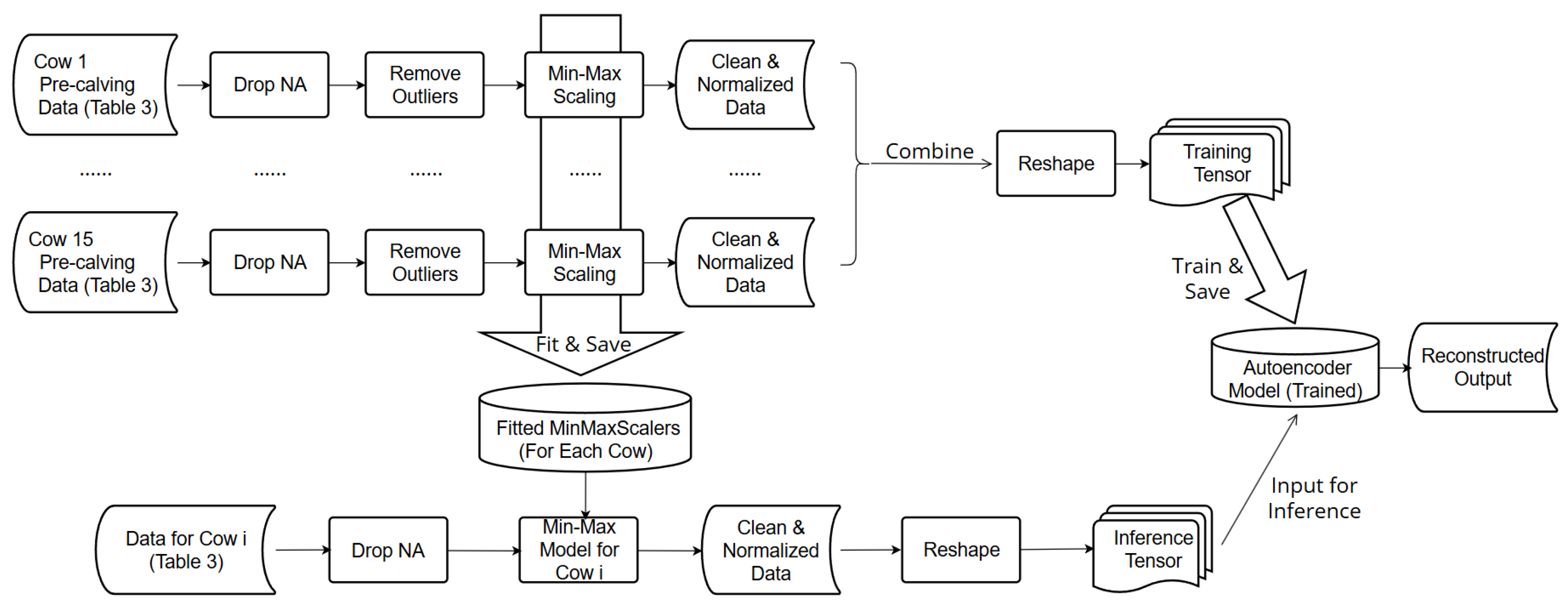
All pre-calving data was cleaned and processed as shown in Figure 3. First, any rows with missing feature values were removed to ensure data integrity. In particular, since we do not have missing values in our raw data, the only missing values are with the generated features MI difference, walking distance, and ts in the first instance because these features’ values cannot be calculated without information of the preceding MI and location before the first instance. Thus, this step just needs to remove the first row. Second, outliers for each feature class were identified and excluded. Outliers were detected using the inter-quartile range ($IQR$) difference. Briefly, we computed the first and third quartiles ($Q1$ and $Q3$, respectively) for each feature, calculated the $IQR$, and determined the lower and upper bound as follows:

$$IQR=Q3-Q1$$

$$\mathrm{Lower}\mathrm{bound}=Q1-1.5IQR$$

$$\mathrm{Upper}\mathrm{bound}=Q3+1.5IQR$$

where the Lower bound and Upper bound represent the lower and upper limits for outlier detection.

Third, selected features including the motion index, walking distance, sum of KNN1–KNN3, and $ts$ were normalized for each cow using the Min–Max scaling procedure [26]. The Min–Max scalers were then saved for application with the test data.

After the cleaning and normalization steps, the pre-calving data were merged to a single file and used to train the autoencoder. An input instance to the autoencoder comprises six features: (1) normalized motion index, (2) normalized walking distance, (3) normalized sum of KNN1-KNN3, (4) normalized ts, (5) time encoding hour_sin, and (6) hour_cos. These data were organized into a 2D tensor of shape with a format $N\times 6$, where N is the number of time points across all cows, and 6 is the number of features used. The data was passed to the autoencoder in batches.

The encoder comprises two linear layers. The first layer maps the 6 features to 32 hidden units, being followed by an ReLU activation. The second layer compresses the representation to 16 hidden units. The decoder mirrors this structure, reconstructing the input from the compressed representation through two fully connected layers with corresponding ReLU activations. The autoencoder utilizes the DataLoader from pytorch 2.6.0+cu124. The batch size is 64 with shuffle set to be True. The learning rate is set to be 1 × 10⁻³, and the number of learning epoches is 100.

Importantly, only the first four features (behavioral features) are included in the reconstruction loss. The time encoding features are provided solely as hints to help the model learn time-dependent patterns, but they are not part of the reconstruction objective. During training, we use the L1 loss between the input and reconstructed output, computed only over the four behavioral features. The L1 loss is also called the Mean Absolute Error (MAE) of a prediction. The MAE at the timestamp t is defined as shown in Equation (5).

$$MA{E}_t={\displaystyle \frac{1}{n}}\sum _{i=1}^n\left|y_{it}-{\widehat{y}}_{it}\right|$$

(5)

where $y_{it}$ is the actual value of the ith feature at the timestamp t, ${\widehat{y}}_{it}$ is the reconstructed value of the ith feature at the timestamp t, and n is the number of features used.

The trained autoencoder was intended to capture the regular behavior of cows before calving. To use the autoencoder for predictions, additional processing steps of the input data were required. These processing steps (bottom box in Figure 3) uses the previously processed data show in Table 3. The input data includes both pre-calving- and calving-related data. In a following step, data were cleaned and normalized. The normalization was applied using the Min–Max scalers learned previously from the pre-calving data, ensuring the consistent normalization of all data. Finally, because calving events are abnormal events, the “Remove outliers” step was not utilized (Figure 3). Similar to the training data, the testing data needs to be processed to the same format before it is fed into the model. Therefore, the format of the testing data was the same as the training data described before.

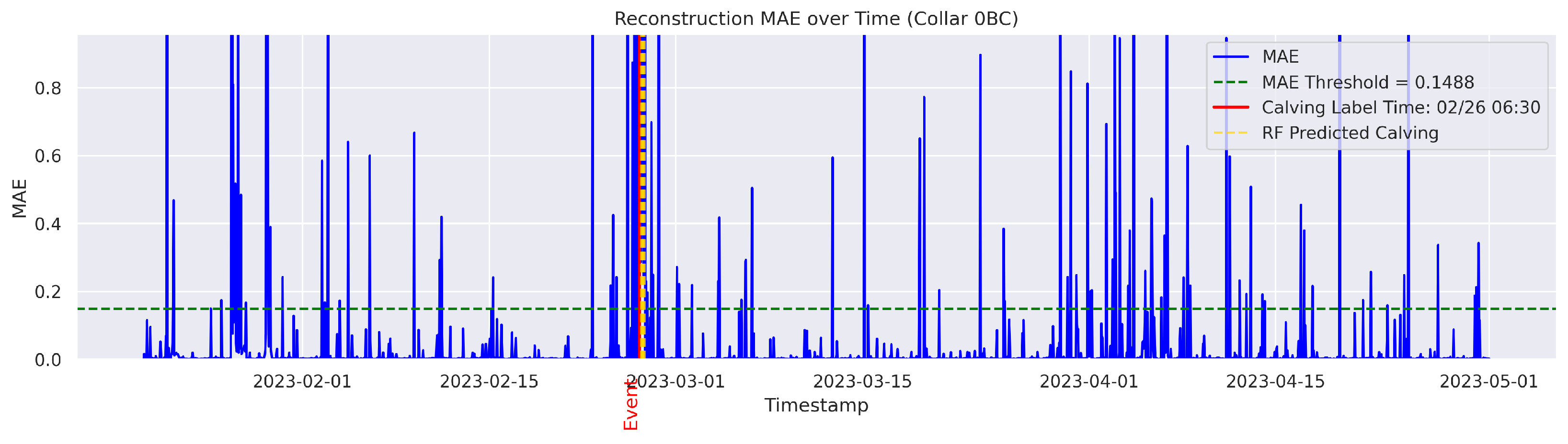
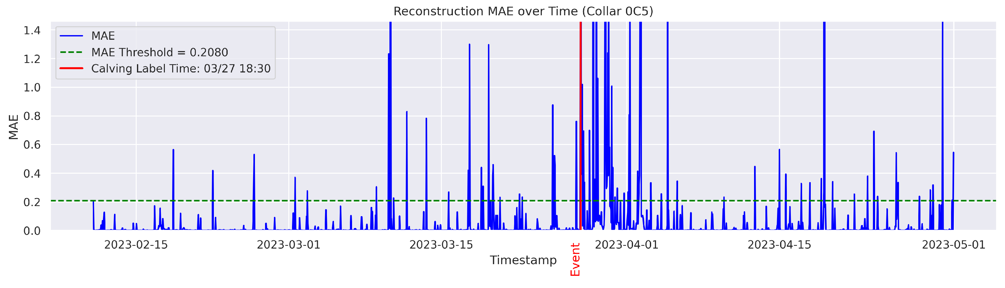
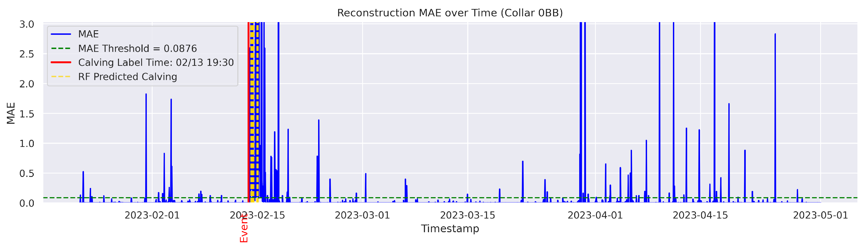
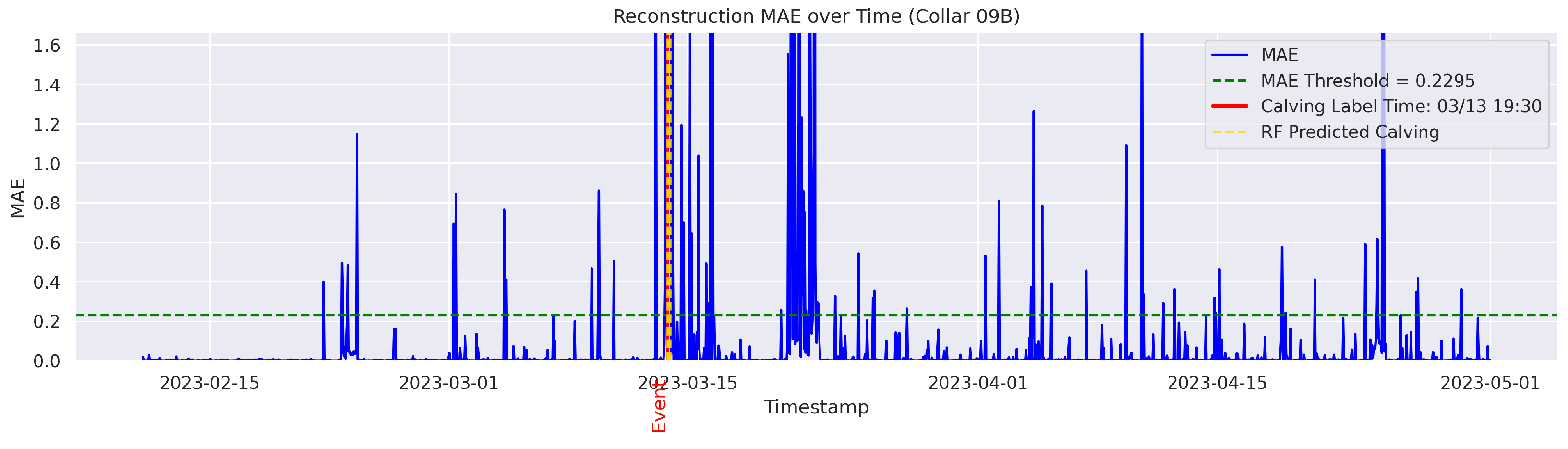
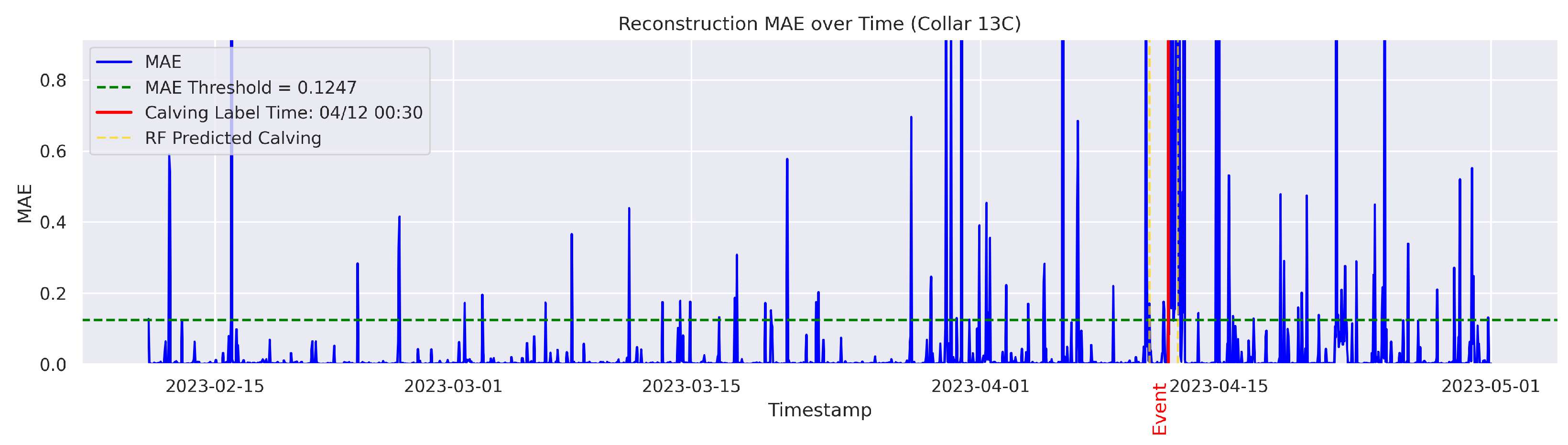
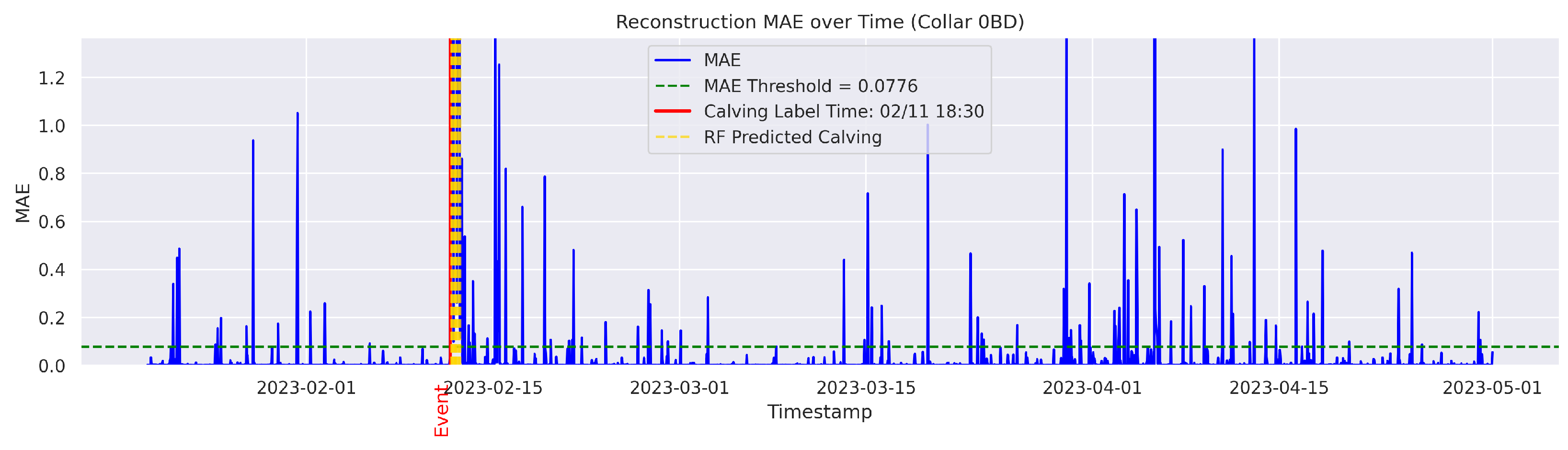
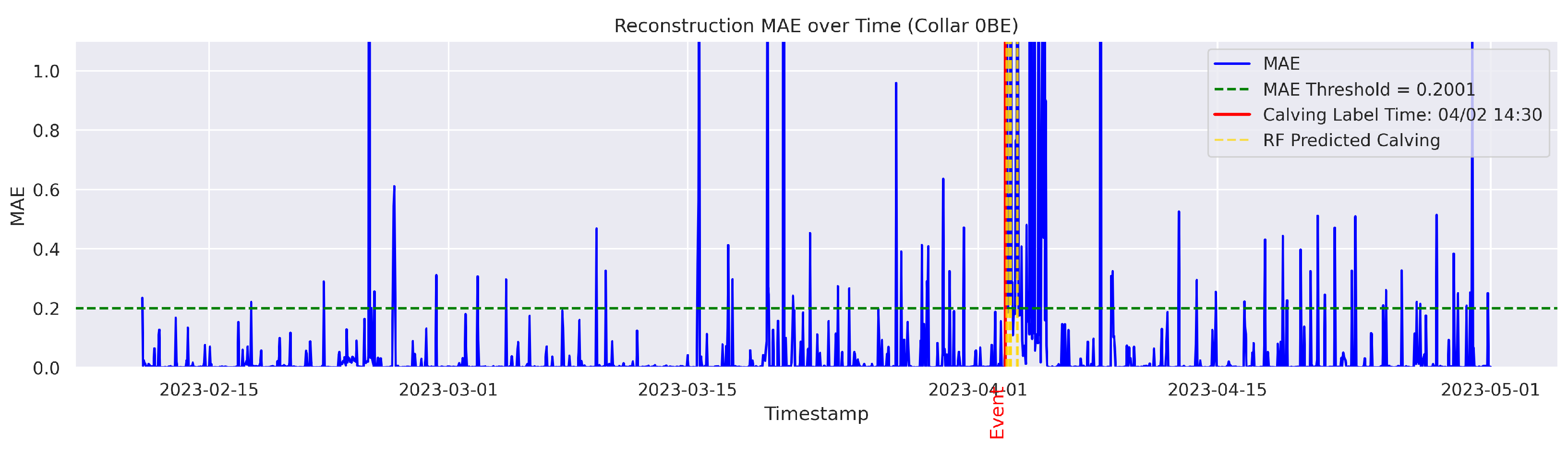
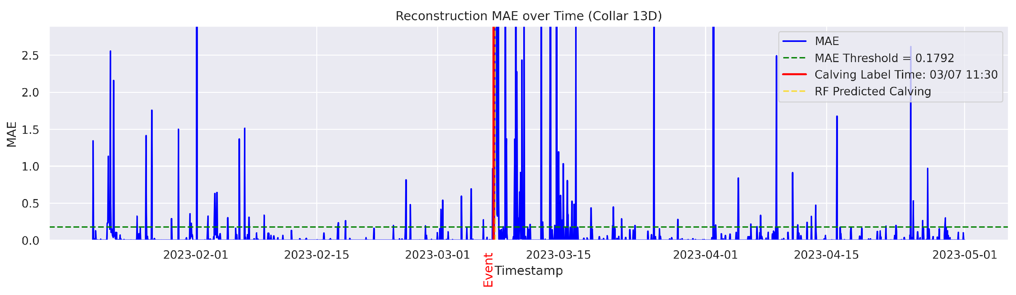
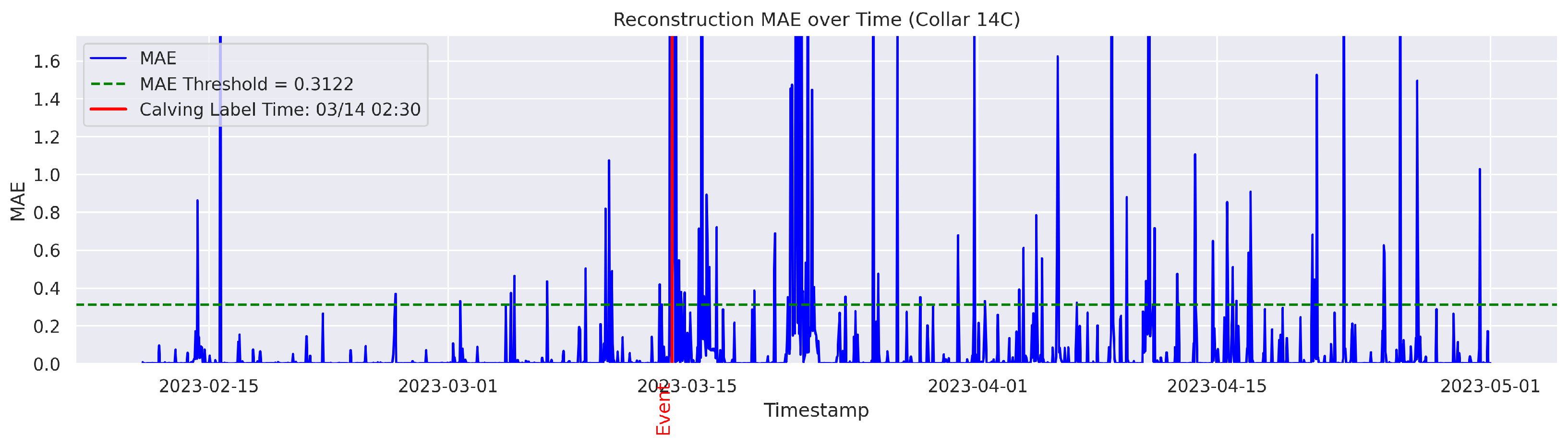
The following procedure was used to identify anomalous data points using the autoencoder. At each timestep t, the autoencoder predicts the values of all features. These predicted values are then compared to the actual values. It is important to note that the time encoding features are not part of the reconstruction objective. To quantify the difference, also known as the reconstruction error [27], we used the MAE. If the MAE at a timestamp t exceeds a predefined threshold, the corresponding timestamp t is flagged as an instance of abnormal behavior. The MAE was utilized because it directly measures the average magnitude of errors in the same units as the data, making it intuitive and easy to understand; it also avoids overemphasizing large outliers compared to the Mean Squared Error (MSE). The threshold for anomaly detection was set to the 95th percentile of the reconstruction error. Therefore, time points with a higher MAE value were considered anomalous.

The output data had the same number of rows as the input data. The columns included were “Rounded UTC Time”, “Threshold”, “MAE”, and the boolean value “Anomaly”, which was derived based on the comparison between the set threshold and the MAE value. An example of the output data is shown in

Table 4. Output for a cow with ID “OBA”.

Rounded UTC Time	Threshold	MAE	Anomaly
2023-02-11 02:00:00+00:00	0.1876	0.1134	FALSE
2023-02-11 03:00:00+00:00	0.1876	0.0034	FALSE
...	...	...	...

.

3.2. Stage 2: Classification of Calving Events

The goal of this stage was to distinguish abnormal points associated with calving from those caused by other behaviors. To this end, we implemented a supervised Random Forest (RF) classification model. The RF was selected over alternative models due to its robustness to noisy data, ability to handle imbalanced datasets, and effectiveness in capturing complex nonlinear relationships between features [28], which are characteristic of this dataset. Preliminary inspection revealed a highly imbalanced dataset, with relatively few “calving” anomalies (True) compared to “non-calving” anomalies (False), which may bias a classifier toward the majority class. Additionally, calving labels were assigned by observers based on frequent but discontinued field observation schedules. This procedure may introduce noise, reducing the labeling accuracy. This bias may also obscure detecting relevant patterns, limiting the model’s ability to reliably distinguish calving events from other irregular activities.

Finally, RF provides a feature relevancy rank, enhancing the overall interpretability and helping to identify the most relevant features for classification. These properties make RF a particularly suitable classifier for our application.

The method was implemented in three steps. The first step is to label feature data with corresponding calving and non-calving labels. To this end, anomalous data points identified near the observed calving time (ground-truthed calving time) were labeled as “calving” (True). In contrast, anomalous detected points that were not associated with a true calving event were labeled as “non-calving” (False). For labeling purposes, we defined ‘near calving time’ as any time point within 24 h (±1 day) of the ground-truthed calving time. The use of a selective range was decided to mitigate any bias from field observers by ensuring that only data points proximate to the true calving event were included in the calving label. The resulting labeled dataset was subsequently partitioned into training and testing sets.

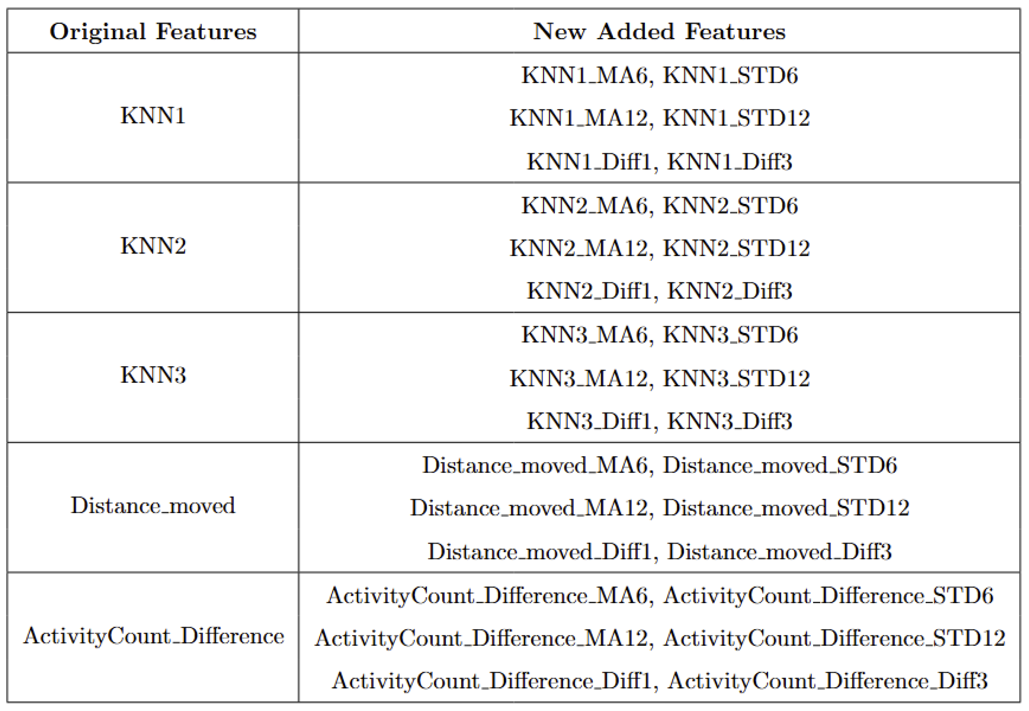
The second step was to train the RF classifier using labeled data. Prior to training, we enriched the original features by applying a sliding window function to capture short-term behavioral trends. This method computes moving averages (MAs) and standard deviations (STDs) over recent time windows (e.g., 6 and 12 h), as well as short-term differences (e.g., 1- and 3-h differences) for each of the core behavioral features. The added statistical context improves the classifier’s ability to distinguish calving-related anomalies from other outliers. Each instance has a total of 35 features used for classification, the list of features can be found in Appendix B.

The RF is composed of multiple decision trees and decision tree splits based on the value of the features. These splits do not rely on euclidean distance or other distance-based metrics; therefore, the scale or distribution of features does not affect the splitting rules. The splits are based on the relative order of feature values rather than their absolute magnitudes or the distances between them [28]. This approach eliminates the need for additional processing steps, such as standardization, preserving the original meaning and interpretability of the features. The RF model was initialized with 100 decision tree estimators; take $n\_estimators=100$, and the class weights were set to “balanced” ($class\_weight=‘\mathrm{balanced}’$) to account for the inherent class imbalance between calving and non-calving events. The “balanced” mode automatically considers the weight of each class to be inversely proportional to its frequency [29], ensuring that the minority class (calving) receives more attention during training. Without class weighting, the classifier could achieve superficially high accuracy by simply predicting all samples as non-calving. For example, always predicting the majority class could result in over 95% accuracy yet completely fail to identify any calving events. Such behavior would be unacceptable, as missing calving events is far more costly than generating false alarms. All the other parameters take the default values set in the random forest function from the scikit-learn package.

The last step was to make predictions on the testing dataset to verify the performance of the classifier.

3.3. Evaluation Metrics

To evaluate the performance of the proposed method, we adopted standard binary classification metrics, including True Positive (TP), False Positive (FP), True Negative (TN), and False Negative (FN) metrics. A prediction is considered a TP if it correctly identifies a calving event. A FP occurs when the model incorrectly predicts a calving event at a non-calving time. A TN refers to a correctly predicted non-calving instance, while a FN is a calving event that the model fails to detect.

Based on these definitions, we computed three standard evaluation metrics. The Precision measures the proportion of predicted calving events that are correct and is defined as $Precision={\displaystyle \frac{TP}{TP+FP}}$. The Recall quantifies the proportion of actual calving events that are successfully detected by the model and is defined as $Recall={\displaystyle \frac{TP}{TP+FN}}$. The F1-score is the harmonic mean of precision and recall and is computed as $F1=2·{\displaystyle \frac{Precision·Recall}{Precision+Recall}}$. These metrics collectively provide a comprehensive reference of the model’s effectiveness in detecting calving events.

3.3.1. Evaluation Metrics for Anomaly Detection in Stage 1

The primary goal of the anomaly detection is to ensure that calving is successfully detected and without omission of any true calving event. In particular, high Recall values are preferred, meaning that data points related to true calving points are correctly identified as anomalous. We also noted other anomalies associated with low locomotion, health issues, or changes in behavior associated with inclement weather. Therefore, as our label data only includes calving events but no other events that may cause cows to behave abnormally, it is not realistic to expect a high precision.

Cows were observed twice daily at approximately 12-h intervals; therefore, calving labels may not be 100% accurate. In some cases, the recorded calving time reflects the best possible estimate based on field staff observations and judgment. To mitigate uncertainty, a time range was applied. The model predictions were considered TPs if they occurred within 24 h before or after the annotated calving time. This approach therefore accounts for the twice-daily cow inspection schedule used in this study.

3.3.2. Evaluation Metrics for Classifications in Stage 2

The goal was to distinguish calving-related anomalies from all the other detected anomalies. Therefore, Precision becomes more important in this stage. It is worth noting that the behavioral patterns associated with calving may not immediately return to normal after the event. The anomalous behaviors related to calving may persist for several hours post calving. As a result, we clustered the classifier’s predictions for calving-related anomalies based on temporal proximity. Predictions made by the classifier were grouped into clusters if their timestamps fell within a predefined temporal threshold (e.g., within 24 h of each other). Each cluster represented a single event as identified by the classifier. Following this criterion, if the point closest to the actual calving time within a cluster was classified as a TP, the entire cluster was labeled as a TP; otherwise, the cluster was classified as an FP.

We split the data by cow into training and testing sets. We performed a 5-fold cross-validation, where, in each iteration, 12 cows were used for training and the remaining 3 cows were used for testing. This process ensures that each cow is used for both training and testing across different folds, providing a robust evaluation of the model’s performance.

4. Results and Discussion

4.1. Results for Anomaly Detection in Stage 1

The results of the detected abnormal behaviors are presented in

Table 5. Results of anomalous event detection using autoencoder in stage 1.

ID	Recall	Anomalies Detected	Total Time Points
0BA	1.0	94	1876
0BB	1.0	118	2358
0BE	1.0	95	1885
0E1	1.0	95	1886
12B	1.0	94	1880
09B	1.0	95	1890
0BD	1.0	121	2415
0C5	1.0	95	1890
0E7	1.0	121	2410
12A	1.0	118	2358
09F	1.0	120	2402
13C	1.0	94	1882
0BC	1.0	121	2409
13D	1.0	121	2405
14C	1.0	94	1882

. This table summarizes the number of anomalies detected along with the total number of data points and the prediction Recall for each of the cows (Table 5).

The method demonstrated high accuracy in detecting significant changes in behavior patterns during calving-related events. These change points aligned well with observable deviations in cow activity. The detailed prediction for each cow using the autoencoder can be found in Appendix A.

From these results, it can be observed that the autoencoder demonstrates a high recall performance, as expected. Additionally, the autoencoder evaluated each data point individually. Therefore, it was effective to filter out a subset of data points for training the RF classifier in stage 2.

4.2. Results for Classification in Stage 2

The results in

Table 6. Results of calving event classification in stage 2.

ID	Precision	Recall	F1 Score	Time_Gap (h) 1
0BA	1.0	1.0	1.00	0.0
0BB	1.0	1.0	1.00	8.0
0BE	1.0	1.0	1.00	2.0
0E1	1.0	1.0	1.00	5.0
12B	1.0	1.0	1.00	14.0
09B	1.0	1.0	1.00	0.0
0BD	1.0	1.0	1.00	3.0
0C5	0.0	0.0	0.00	NaN
0E7	1.0	1.0	1.00	3.0
12A	0.0	0.0	0.00	47.0
09F	0.5	1.0	0.67	2.0
13C	1.0	1.0	1.00	14.0
0BC	1.0	1.0	1.00	3.0
13D	1.0	1.0	1.00	5.0
14C	0.0	0.0	0.00	NaN

¹ Time_Gap represents the minimum time difference between the predicted calving event and the label.

report the testing results from the five-fold cross-validation. These results include the classifier performance metrics Precision, Recall, and F1 Score for each of the cows along with the temporal gap in hours between the observed and predicted onset of calving.

The performance of the classifier was evaluated individually for all 15 cows. Among them, 12 cows (80%) were correctly identified and classified. From these 12 cows, only 1 cow (with id 09F) had one False Positive, resulting in the 0.5 precision. All the other cows had zero False Positives. Reducing False Positive detections is critical, as inaccurate or untimely alerts—either too early or too late—can result in missed opportunities to detect the true onset of calving in a timely manner.

The cows with calving time correctly detected and classified included the IDs 0BA, 0BB, 0BE, 0E1, 12B, 09B, 0BD, 0E7, 13C, 0BC, 13D, and 09F. For these cows the two-phase autoencoder and Random Forest model achieved a combined performance of 100% Recall for event detection and 96% Precision for correct classification, respectively. These performance metrics suggest promise for the combination of unsupervised and supervised modeling on position and movement data collected in real-time to detect calving of cows in open rangelands. Furthermore, in this study the aim was to apply real-time animal tracking and implement unsupervised and supervised machine learning on tracking data to accurately detect calving of cows grazing large rangeland pastures. No comparisons were conducted with other sensor platforms used for the collection of tail [10], leg [12], and neck [11] movements. Such sensor platforms typically consist of store-on-board devices or passive devices with delayed data transmission, which may limit applications for real-time animal tracking on large open rangeland. Likewise no direct comparisons to other Random Forest or deep learning models were conduced. However, the performance metrics for Precision and Recall for these cows were comparable, and even better, compared to a Precision of 65% for a Random Forest model [12]. Other machine learning models, trained either on neck, leg, or tail sensor data, report a similar performance metric [11]. Furthermore, high Precision (85–92%) and Recall (91–95%) ranges have been reported previously for deep learning models that have utilized either CNN, RNN, or hybrid approaches such as C-LSTM [12] or C-BiLSTM [10] trained on different sensor datasets.

On the other hand, the model failed to detect and classify calving for the cows 0C5, 12A, and 14C. In this study, a classification failure was explicitly defined as either a missed detection for the autoencoder or an incorrect classification of a calving anomaly by the Random Forest model. Likewise a missed detection or misclassification refers to any observed calving event that is either not identified or identified outside a 24-h window from the ground-truthed calving time. Therefore, the cows 0C5, 12A, and 14C yielded no true calving detection and classification (Precision = 0%; Recall = 0%), indicating a complete failure of the classifier. Interestingly, the inspection of the data indicated that their behavior patterns differed from all other cows. These cows calved near the water point and therefore did not exhibit a persistent tendency for social isolation before, during, or after calving. The behavior and distribution patterns of 12A and 14C were rarely observed in the training set, which may have limited the model’s ability to learn the specific patterns associated with these cases. These observations are consistent with findings of previous studies that have documented ample variability of movement behavior and isolation trends among parturient beef cows [30]. Age, personality, temperament, animal breed, and nutritional status may partially explain such differences [31]. Fusing data from distinct sensor platforms (i.e., tail sensors, body temperature sensors, heart rate sensors, etc.) capable of capturing different dimensions of animal behavior and physiology around calving could be used to mitigate individual variability for accurate calving detection [32]. These methods may offer a more broad application of distinct sensor platforms for the detection of calving at pasture where animal behavior is likely to vary significantly from cow to cow. The cow 12A had a recall of 0% and a time gap of 47 h between the detected anomaly and the ground-truth label, exceeding the one-day (24 h) threshold and thus considered a failed case to detect the onset of calving in a timely manner.

The detailed prediction for each cow using the Random Forest classifier can be found in Appendix A. The results demonstrated that, from a practical standpoint, false calving alerts can be minimized through the combination of unsupervised and supervised machine learning techniques. Additionally, up to 80% of calving events were successfully detected and classified, providing ranchers with early indications of calving onset. However, the model’s performance appears to be highly dependent on the behavior and distribution patterns of periparturient cows at pasture, highlighting the need to evaluate its predictive capability across different pastures, herd sizes, and environmental conditions that influence the behavior and distribution of animals at pasture [16,32].

5. Conclusions

This study investigated methods for detecting calving events in cattle, a key component of precision livestock management. Effective monitoring of parturient cows is essential to reducing cow and calf mortality, improving reproductive and production performance, and minimizing labor costs. However, traditional monitoring protocols face substantial challenges, especially in large-scale ranch operations where frequent cattle inspections require driving long distances, often over difficult terrain. These time, cost, and logistical constraints limit the practicality of traditional human-based monitoring approaches. To overcome these limitations, we implemented a long-range, low-power sensor network to monitor cattle behavior in real-time. This system was coupled with a two-stage calving detection framework combining an unsupervised anomaly detection model and a supervised classification model. In the first stage, an autoencoder was used to model the normal cow behavior and identify both calving and non-calving anomalies. In the second stage, a Random Forest classifier was employed to determine whether these anomalies were indicative of a calving event. While the proposed method demonstrated promising results and contributed to the advancement of calving detection techniques, opportunities for improvement remain. Future work could explore the implementation of adaptive thresholding strategies of the autoencoder and further optimization of hyperparameters. Additionally, enhancing the generalizability, scalability, and robustness of this system across diverse cattle breeds, pasture types, and management strategies is critical to advance progress.

6. Future Perspectives

The current method has shown promising results in detecting calving events in beef cows managed on a open rangeland pasture; nonetheless, additional validation is required to assess its generalizability and applicability across varied environmental conditions, breeds of cows, cattle management systems, and animal housing methods.

The current autoencoder architecture and training settings (e.g., number of layers, hidden units, learning rate, and batch size) may not be fully optimized for the present dataset or anomaly detection tasks. Future work could fine tune these values to achieve better calving detection results.

Another line of research could focus on evaluating the model’s generalization. For instance, it would be valuable to assess whether a model trained on data from a specific group of cows or a particular pasture can be directly applied to data collected from different cattle populations varying in temperament, age, herd size, or breed. Pastures with differing vegetation types, terrain complexity, and climatic conditions can influence animal behavior and distribution significantly, affecting model performance and generalizability. Therefore, studies conducted across different pasture settings must be compared. Additionally, the influence of management practices, such as strategic supplementation, water placement, and rotational grazing, could be systematically tested. Finally, domain adaptation strategies, including transfer learning or fine-tuning, may offer promising approaches to improve the model’s applicability across diverse grazing and management environments.

References

1. U.S. Department of Agriculture Climate Hubs. Precision Ranching in the Southwest. Available online: https://www.climatehubs.usda.gov/hubs/southwest/topic/precision-ranching-sw (accessed on 26 November 2024).
2. Johanson, J.M.; Berger, P.J. Birth weight as a predictor of calving ease and perinatal mortality in Holstein cattle. J. Dairy Sci. 2003, 86, 3745–3755. [Google Scholar] [CrossRef] [PubMed]
3. Scasta, J.D.; Windh, J.L.; Stam, B. Modeling large carnivore and ranch attribute effects on livestock predation and nonlethal losses. Rangel. Ecol. Manag. 2018, 71, 815–826. [Google Scholar] [CrossRef]
4. Crociati, M.; Sylla, L.; Monaci, M. How to Predict Parturition in Cattle? A Literature Review of Automatic Devices and Technologies for Remote Monitoring and Calving Prediction. Animals 2022, 12, 405. [Google Scholar] [CrossRef] [PubMed]
5. Ricci, A.; Racioppi, V.; Iotti, B.; Bertero, A.; Reed, K.F.; Pascottini, O.B.; Vincenti, L. Assessment of the temperature cut-off point by a commercial intravaginal device to predict parturition in Piedmontese beef cows. Theriogenology 2018, 113, 27–33. [Google Scholar] [CrossRef]
6. Horváth, A.; Lénárt, L.; Csepreghy, A.; Madar, M.; Pálffy, M.; Szenci, O. A field study using different technologies to detect calving at a large-scale Hungarian dairy farm. Reprod. Domest. Anim. 2021, 56, 673–679. [Google Scholar] [CrossRef]
7. Schirmann, K.; Chapinal, N.; Weary, D.M.; Vickers, L.; Von Keyserlingk, M.A.G. Rumination and feeding behavior before and after calving in dairy cows. J. Dairy Sci. 2013, 96, 7088–7092. [Google Scholar] [CrossRef]
8. Chang, A.Z.; Imaz, J.A.; González, L.A. Calf birth weight predicted remotely using automated in-paddock weighing technology. Animals 2021, 11, 1254. [Google Scholar] [CrossRef]
9. Giaretta, E.; Marliani, G.; Postiglione, G.; Magazzù, G.; Pantò, F.; Mari, G.; Formigoni, A.; Accorsi, P.A.; Mordenti, A. Calving time identified by the automatic detection of tail movements and rumination time, and observation of cow behavioural changes. Animal 2021, 15, 100071. [Google Scholar] [CrossRef]
10. Yang, L.; Zhao, J.; Ying, X.; Lu, C.; Zhou, X.; Gao, Y.; Wang, L.; Liu, H.; Song, H. Utilization of deep learning models to predict calving time in dairy cattle from tail acceleration data. Comput. Electron. Agric. 2024, 225, 109253. [Google Scholar] [CrossRef]
11. Miller, G.A.; Mitchell, M.; Barker, Z.E.; Giebel, K.; Codling, E.A.; Amory, J.R.; Michie, C.; Davison, C.; Tachtatzis, C.; Andonovic, I.; et al. Using animal-mounted sensor technology and machine learning to predict time-to-calving in beef and dairy cows. Animal 2020, 14, 1304–1312. [Google Scholar] [CrossRef]
12. Liseune, A.; Van den Poel, D.; Hut, P.R.; van Eerdenburg, F.J.C.M.; Hostens, M. Leveraging sequential information from multivariate behavioral sensor data to predict the moment of calving in dairy cattle using deep learning. Comput. Electron. Agric. 2024, 225, 109253. [Google Scholar] [CrossRef]
13. Sumi, K.; Zin, T.T.; Kobayashi, I.; Horii, Y. Framework of cow calving monitoring system using a single depth camera. In Proceedings of the 2018 International Conference on Image and Vision Computing New Zealand (IVCNZ), Auckland, New Zealand, 19–21 November 2018; pp. 1–7. [Google Scholar]
14. Hyodo, R.; Nakano, T.; Ogawa, T. Feature representation learning for calving detection of cows using video frames. In Proceedings of the 2020 25th International Conference on Pattern Recognition (ICPR), Milan, Italy, 10–15 January 2020; pp. 4131–4136. [Google Scholar]
15. Mg, W.H.E.; Zin, T.T.; Pyke, T.; Aikawa, M.; Honkawa, K.; Horii, Y. Automated system for calving time prediction and cattle classification utilizing trajectory data and movement features. Sci. Rep. 2025, 15, 2378. [Google Scholar] [CrossRef] [PubMed]
16. García García, A.J.; Maroto Molina, F.; Pérez Marín, C.C.; Pérez Marín, D.C. Potential for automatic detection of calving in beef cows grazing on rangelands from Global Navigate Satellite System collar data. Animal 2023, 17, 100901. [Google Scholar] [CrossRef] [PubMed]
17. New Mexico State University. Facilities: Chihuahuan Desert Rangeland Research Center. Available online: https://chihuahuansc.nmsu.edu/research/facilities.html (accessed on 26 November 2024).
18. Perea, A.; Rahman, S.; Nyamuryekung’e, S.; Chen, H.; Bakir, M.; Cox, A.; Cao, H.; Estell, R.; Bestelmeyer, B.; Cibils, A.F.; et al. Integrating LoRaWAN sensor networks and machine learning models to classify beef cattle behavior on arid rangelands of the southwestern United States. Smart Agric. Technol. 2025, 11, 101002. [Google Scholar] [CrossRef]
19. McIntosh, M.M.; Cibils, A.F.; Nyamuryekung’e, S.; Estell, R.; Cox, A.; Duni, D.; Gong, Q.; Waterhouse, T.; Holland, J.P.; Cao, H.; et al. Deployment of a LoRa-WAN near-real-time precision ranching system on extensive desert rangelands: What we have learned. Appl. Anim. Sci. 2023, 39, 349–361. [Google Scholar] [CrossRef]
20. Pandas Development Team. Pandas.DataFrame.Fillna—Pandas 2.0.3 Documentation. Available online: https://pandas.pydata.org/pandas-docs/stable/reference/api/pandas.DataFrame.fillna.html (accessed on 26 November 2024).
21. GeeksforGeeks. Haversine Formula to Find Distance Between Two Points on a Sphere. Available online: https://www.geeksforgeeks.org/haversine-formula-to-find-distance-between-two-points-on-a-sphere/ (accessed on 26 November 2024).
22. Vaswani, A.; Shazeer, N.; Parmar, N.; Uszkoreit, J.; Jones, L.; Gomez, A.N.; Kaiser, L.; Polosukhin, I. Attention is all you need. In Proceedings of the Advances in Neural Information Processing Systems, Long Beach, CA, USA, 4–9 December 2017; pp. 5998–6008. [Google Scholar]
23. Bengio, Y.; Courville, A.; Vincent, P. Representation Learning: A Review and New Perspectives. IEEE Trans. Pattern Anal. Mach. Intell. 2013, 35, 1798–1828. [Google Scholar] [CrossRef]
24. Goodfellow, I. Deep Learning; The MIT Press: Cambridge, MA, USA, 2016. [Google Scholar]
25. Provotar, O.I.; Linder, Y.M.; Veres, M.M. Unsupervised anomaly detection in time series using LSTM-based autoencoders. In Proceedings of the 2019 IEEE International Conference on Advanced Trends in Information Theory (ATIT), Kyiv, Ukraine, 18–20 December 2019; pp. 513–517. [Google Scholar]
26. Scikit-learn. Sklearn.Preprocessing.MinMaxScaler. Available online: https://scikit-learn.org/1.5/modules/generated/sklearn.preprocessing.MinMaxScaler.html (accessed on 26 November 2024).
27. Willmott, C.J.; Matsuura, K. Advantages of the mean absolute error (MAE) over the root mean square error (RMSE) in assessing average model performance. Clim. Res. 2005, 30, 79–82. [Google Scholar] [CrossRef]
28. Breiman, L. Random forests. Mach. Learn. 2001, 45, 5–32. [Google Scholar] [CrossRef]
29. Scikit-learn. Random Forest Classifier. Available online: https://scikit-learn.org/stable/modules/generated/sklearn.ensemble.RandomForestClassifier.html (accessed on 14 April 2025).
30. Flörcke, C.; Grandin, T. Separation Behavior for Parturition of Red Angus Beef Cows. Open J. Anim. Sci. 2014, 4, 43–50. [Google Scholar] [CrossRef]
31. Zuko, M.; Jaja, I.F. Primiparous and multiparous friesland, jersey, and crossbred cows’ behavior around parturition time at the pasture-based system in South Africa. J. Adv. Vet. Anim. Res. 2020, 7, 290–298. [Google Scholar] [CrossRef]
32. Chang, A.Z.; Swain, D.L.; Trotter, M.G. Towards sensor-based calving detection in the rangelands: A systematic review of credible behavioral and physiological indicators. Transl. Anim. Sci. 2020, 4, txaa155. [Google Scholar] [CrossRef]
Figure 1. The CDRRC consist in 64,000 acres of desert grassland and shrubland extending across the Jornada del Muerto basin in southern New Mexico.
Agriculture 15 01434 g001
Figure 2. Map of the study site and cattle used in this study. (a) Map of the CDRRC showing the 700 ha study pasture (solid blue area). (b) Brangus cow with tracking collar used in this study.
Agriculture 15 01434 g002
Figure 3. Data processing steps prior to implementing the autoencoder.
Agriculture 15 01434 g003