1. Introduction
Farmland plots serve as the foundation of agricultural production [
1,
2]. Timely, accurate, and efficient extraction of farmland plots is of major significance for developing scientifically sound agricultural planning and farmland plot management. Traditional methods such as visual interpretation and manual field surveys for extracting farmland plots are costly and time-consuming and cannot meet the demands of large-scale and rapidly updated farmland plot extraction [
3,
4]. With technological advancements, using remote sensing images for the intelligent extraction of farmland plots offers advantages such as wide coverage, efficiency, speed, and low cost [
5,
6]. Therefore, numerous scholars worldwide have conducted extensive research in this area, yielding significant results and making intelligent remote sensing technology a timely, accurate, and efficient means of farmland plot extraction [
7,
8,
9].
Internationally, European countries and the United States have always been important areas in the field of farmland plot extraction. In 1979, the Agristars project was implemented by the U.S. Department of Agriculture, with farmland plot extraction as a significant component of this project, involving a large-scale extraction of farmland plots in the United States and Canada. Their extraction method primarily relied on manual delineation with machine automation as a supplement, thus achieving the optimal balance between manual extraction and automatic mapping [
10]. In the 1980s, scholars such as Pitts began exploring the use of automated extraction algorithms combined with satellite imagery to extract farmland plots, providing a certain theoretical foundation for research related to the automated extraction of farmland plots [
11]. After a long period of theoretical exploration and technological accumulation, the extraction of farmland plots has transitioned from traditional visual interpretation methods to semi-automated or even automated methods. In 1999, Rydberg, A, and others proposed a multispectral edge detection method that combines various optimal techniques, using amplitude and direction information to enhance edges, remove noise, and detect edges between regions with different spectral features, suitable for multi-temporal and multispectral image analysis [
12]. In 2001, Rydberg et al. [
13] proposed a method that successfully combined edge detection with segmentation algorithms to extract farmland plots from multispectral images. This study demonstrated that low spatial resolution remote sensing images (such as Landsat), due to their advantage of having more bands, could help researchers achieve higher accuracy in extracting farmland plots than using high-spatial-resolution remote sensing images (such as Systeme Probatoire d’Observation de la Terre, SPOT) [
13]. In 2014, Yan and Roy used a long time series of Landsat Normalized Difference Vegetation Index (NDVI) images, combined with edge detection and morphological post-processing of the extraction results, to achieve the automated extraction of farmland plots [
14]. In 2019, Leila Maghsoodi et al. developed an area-based model from nonparametric active contour models for agriculture land boundary extraction from IRS P5 satellite images [
15]. In 2020, Masoud et al. designed a Multiple Dilated Fully Convolutional Network for detecting farmland plot boundaries from Sentinel-2 images with a 10 m resolution [
16]. In 2021, Waldner used a ResUNet, a deep convolutional neural network, which features a fully connected U-Net backbone with dilated convolutions and conditional inference, to identify and extract individual wheat fields on a large scale [
17]. Meanwhile, the traditional Canny edge detection, Hough transform, and Suzuki85 contour algorithms were used in the land boundary extraction algorithm developed by Rokgi Hong, and the accuracy and completeness rate of the boundary recognition was about 80% in a Korean experiment on regular field boundary extraction [
18]. Developed countries in Europe and the United States have established a relatively mature technical and application service system for extracting farmland plots using medium- to high-resolution remote sensing images after decades of technological accumulation [
19,
20].
Compared to developed countries, China started extracting farmland plot data relatively late, but has experienced rapid technological development. As early as 1996, Ji began using dynamic wavelet algorithms to semi-automatically extract farmland plots from Landsat Thematic Mapper images in the Panyu area of Guangdong Province, opening a new chapter in the research of farmland plot extraction technology in China [
21]. In recent years, machine learning algorithms, such as the maximum likelihood [
22], random forest [
23], support vector machine (SVM) [
24], and decision tree classification [
24] methods, as well as the Neural Network Algorithm [
25], have been successively applied to the extraction of farmland plots, achieving good results. In 2011, Shen et al. used the parallel mean shift algorithm to achieve precise extraction of agricultural and forestry plot boundaries, significantly improving the speed of image segmentation [
26,
27]. These methods extract low-level features and use minimal semantic information [
28]; however, because of the highly variable spectral signature of farmland plots and the spectral confusion in VHR images, low-level features are less effective, resulting in difficulties in transferring the method both temporally and spatially [
29,
30]. In 2016, China carried out its third agricultural census, marking the first time that remote sensing technology was included as a technical method in census work in China. During this period, the high-precision extraction of farmland plots was conducted using traditional manual digitalization methods.
However, unlike the large farms in European countries and the United States, farmland plots in China are mainly composed of small plots [
31]. Extracting farmland plots using medium-resolution satellite data (such as Landsat and Sentinel series satellites) does not meet the practical needs of farmland plot extraction in China. An urgent need exists for farmland plot extraction technology based on high-resolution remote sensing data [
32,
33]. In particular, the successful launch of China’s first sub-meter high-spatial-resolution satellite, Gaofen-2 (GF-2), in 2014 provided a new development opportunity for relevant research and applications in farmland plot extraction in China [
34,
35,
36]. In 2021, Li et al. proposed a building extraction method for farmland plots based on Google and high-resolution WorldView-2 remote sensing images using an attention-enhanced U-Net, achieving good results in farmland plot extraction [
37]. In 2022, some multi-tasking-based networks, such as BsiNet and SEANet, were used for field boundary detection, and surprisingly, these models have achieved better detection results through the constraints of the additional region task signals [
38,
39]. In 2023, Li et al. used an improved Pyramid Scene Parsing Network and U-Net network model combined with high-resolution data, such as GF-1 data, to achieve fine automatic extraction of farmland plots [
40]. These methods provide new technical approaches for farmland plot extraction. However, with the improvement of resolution, new contradictions and issues have emerged in farmland plot extraction, which are as follows: (1) the delineation and inclusion of farmland paths in high-resolution remote sensing images have become important factors affecting the accuracy of farmland plot extraction; (2) finer spatial texture features lead to low extraction accuracy based on pixel information, resulting in serious salt-and-pepper noise [
41]; and (3) farmland plots exhibit significant phenological characteristics.
To address the aforementioned issues, this study primarily used Gaofen-2 data as the main data source. By using images from four key phenological stages in the study area and their combined temporal images, the joint technology of object-oriented multi-scale segmentation based on high-resolution remote sensing images and a support vector machine (SVM) is applied for farmland plot extraction. This method effectively reduces the dependence of model training on a large number of samples, successfully removes noise points, and significantly improves the accuracy and automation level of farmland plot extraction. The main innovations of this study include the following:
- (1)
Conducting a multi-temporal analysis based on the phenological characteristics of farmland plots to propose an optimal phenological period for farmland plot extraction;
- (2)
Incorporating farmland path information into the model to enhance the accuracy of farmland plot boundary extraction by considering the texture features of high-resolution remote sensing data in farmland;
- (3)
Addressing the salt-and-pepper noise phenomenon in extraction based on pixel information using object-oriented multi-scale segmentation technology to group pixels with similar characteristics into a single research object, effectively suppressing the noise and enhancing the integrity of farmland plot extraction;
- (4)
By integrating the SVM classification algorithm, the dependence on large sample sizes is effectively reduced, allowing for the training of high-accuracy models, even with small sample sizes;
- (5)
Reducing the irregularity of plot boundaries extracted from high-resolution remote sensing images, which are often irregular due to mixed pixels at farmland plot edges, through the use of vector regularization technology to improve the vector boundary accuracy of farmland plots.
The findings of this study can be used to enhance existing farmland plot extraction techniques, and they hold significant scientific potential for advancing the application of high-resolution remote sensing images in precision agriculture, agricultural planning, and farmland plot management.
3. Extraction of Farmland Plots from Object-Oriented High-Resolution Remote Sensing Images
3.1. Overall Technical Workflow for Farmland Plot Extraction
The Gaofen-2 remote sensing images exhibit rich spatial structures and surface texture features, allowing for a more accurate capture of details and edge information of objects, which is conducive to the extraction of farmland plots. The use of traditional pixel-based classification methods often leads to spatial data redundancy, resulting in salt-and-pepper images, thereby reducing classification effectiveness [
44,
45,
46]. Because the extraction of farmland plots requires a high level of completeness in the extracted results, this study proposes a method for extracting farmland plots from high-resolution images using object-oriented multi-scale segmentation and SVM fusion. The basic idea is to comprehensively analyze the differences in characteristics and attributes between farmland plots and other non-farmland plot types, grouping pixels with similar characteristics into a study object, which can effectively remove salt-and-pepper noise and improve the completeness of farmland plot extraction.
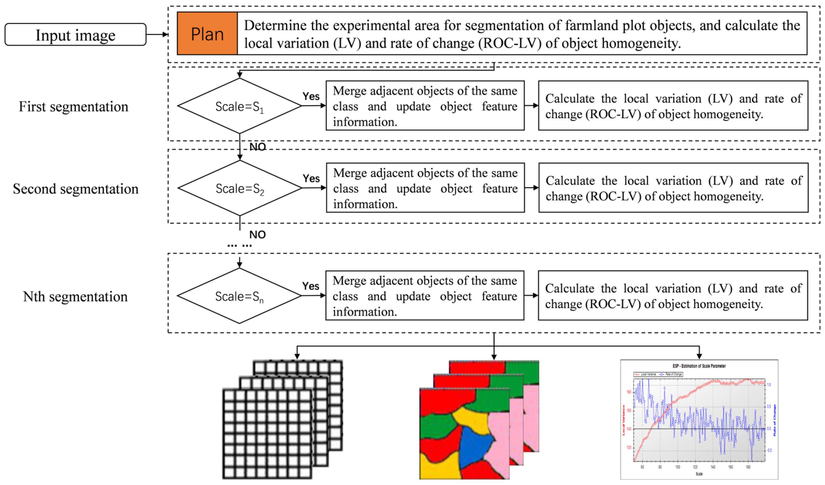
The object-oriented extraction of farmland plots from high-resolution images proposed in this paper mainly includes several important processes, such as determining the optimal extraction time, estimating the optimal segmentation scale parameters, image segmentation, image object construction, selection of classification algorithms, farmland plot extraction, and vector regularization of farmland plots (
Figure 3). Among these, determining the optimal extraction time, estimating the optimal segmentation scale parameters, and constructing the image sample set are core components of the research algorithm, serving as important guarantees for the high-precision extraction of farmland plots.
3.2. Optimal Extraction Time for Farmland Plots
Through experimental image segmentation and a detailed analysis of images over several consecutive months in the same region, it became evident that crop phenology is the primary factor affecting the precision of farmland plot segmentation. Typically, the phenological stages of crops can be divided into stages such as emergence, tillering, jointing, heading, flowering, milk ripening, wax ripening, and full ripening. Taking rice as an example, emergence, tillering, and jointing are classified as the vegetative growth stage, while heading, flowering, milk ripening, and wax ripening are categorized as the reproductive growth stage. Based on these stages, this study selected a satellite image covering 2.24 km
2 of the study area for image segmentation experiments, resulting in the segmentation of the images during the aforementioned stages in the test area (
Figure 4). In the figure, b represents the segmentation result of the unplanted stage, c represents the segmentation result of the vegetative growth stage, and d represents the segmentation result of the reproductive growth stage.
Farmland paths are one of the main boundaries of farmland plots; however, these roads are often earthen and are easily confused with bare soil in unplanted farmland plots, resulting in a significant decrease in segmentation accuracy. Therefore, remote sensing images of unplanted periods are not suitable for farmland plot extraction. Further comparative analysis of the segmentation results of images during the vegetative and reproductive growth stages revealed that using images from the reproductive growth stage yielded better results for farmland plot segmentation than using those from the vegetative growth stage. This occurs because the crop coverage is relatively low during the vegetative growth stage, and small areas of bare soil are present between the rows of crops, leading to lower farmland plot segmentation accuracy. Based on the above research analysis, this study concluded that the optimal time for farmland plot extraction is during the reproductive growth stage of the crops.
3.3. Optimal Segmentation Parameter Estimation for Object-Oriented Image Analysis
Image segmentation is a crucial step in the object-oriented classification process, and the scale parameter of image segmentation is important for classification accuracy. In this study, a multi-scale segmentation algorithm based on object-oriented analysis was employed to segment images during the reproductive growth stage. This algorithm uses the homogeneity criteria of spectral, shape, and spatial texture features of farmland plots for optimal parameter estimation, thereby achieving optimized homogeneous segmentation of the study area images. The main segmentation parameters include band weights, homogeneity factors, and segmentation scales. The technical workflow for determining the segmentation parameters is as follows: (1) set band weights; (2) determine homogeneity factors; and (3) calculate the local variance () and rate of change of local variance () to determine the optimal segmentation scale.
3.3.1. Band Weights
In multi-scale segmentation of remote sensing images, the weights assigned to different bands for segmentation can be determined based on the spectral characteristics of the features to be segmented in each band. If certain features are particularly prominent and easily identifiable in a specific band, the weight assigned to that band can be increased. Image bands that do not contribute significantly to a specific class of information may be assigned smaller weights or a weight of 0.
In this study, the main emphasis of the farmland plot extraction scheme was to use farmland paths to segment large areas of farmland. Considering the relatively low vegetation coverage on farmland paths compared to farmland plots, the strong sensitivity of red and near-infrared bands of the image to vegetation, and experimental exploration experience, the weights of the red and near-infrared bands of the image were set to 2.0, while the weights of the green and blue bands were set to 1.0.
3.3.2. Homogeneity Factor
The quality of image segmentation results depends not only on the segmentation scale and band weights, but also on the following three segmentation attribute factors: compactness, shape, and color parameters, where the sum of the shape and color parameters is 1.
Together, the color and shape parameters determine the homogeneity of objects. Color parameters reflect the spectral characteristics of objects, while shape parameters reflect the textural features of objects. The sum of color and shape parameters is 1. Therefore, when the shape parameter value is too large, it may lead to a loss of spectral information. However, the involvement of shape factors still helps to avoid the incompleteness of the shape of image objects. Compactness parameters are used to differentiate between compact and non-compact targets based on small differences, thereby improving classification accuracy. The relationships among segmentation parameters are shown in the following equations [
47]:
where
represents the weight of color parameters, with a range of [−1, 1];
represents the weight of shape parameters, with a range of [−1, 1]; and the sums of
and
are 1. Additionally,
represents the weight of channel
;
represents the number of pixels of the merged objects;
represent the number of pixels in objects 1 and 2, respectively; and
represents the standard deviation of objects in channel
. Furthermore,
represents the perimeter of the object;
represents the perimeter of the object’s bounding box; the subscript
refers to the merged objects before merging; and
and
refer to objects 1 and 2 before merging, respectively.
In this study, the shape parameter was selected as 0.2 and the compactness parameter was selected as 0.6, based on the spectral and texture features analysis of farmland plots.
3.3.3. Segmentation Scale
The segmentation scale is a crucial factor in the image segmentation process, as it directly determines the size of the image objects. Different segmentation scales result in different sizes and quantities of segmented image objects. A larger or smaller segmentation scale leads to larger or smaller polygon areas and fewer or more objects, respectively. For a specific land cover type, the optimal segmentation scale value can clearly display the boundaries of this land cover type using one or a few objects, without being too fragmented or having blurred edges.
In this study, the principle of selecting the segmentation scale is based on calculating the local variance (
) of homogeneity of farmland plots using different segmentation scale parameters and the rate of change (
) of local variance of segmented objects between the current and previous levels of a scale of interest. This is done to identify the optimal parameter for the segmentation effectiveness of farmland plots. The LV is calculated using the following equation:
where
represents the local variance of the segmented object;
denotes the grayscale value of each pixel; and
represents the mean grayscale value of each object. The ROC is calculated using the following equation:
where
represents the rate of change of
from the
object layer to the
object layer;
is the local variance of the segmented objects at the
object layer; and
is the local variance of the segmented objects at the (
)th object layer.
The process of determining the optimal segmentation scale is an iterative local optimization process. It begins with estimating the number of pixels that should be contained within a given area of farmland to determine that the optimal segmentation scale should fall between S1 and Sn. Then, a small test area of farmland imagery is selected, and multi-scale segmentation experiments are conducted using segmentation scales set within the S1–Sn interval, and with a step size of k. Finally, the
and
values corresponding to each segmentation scale are calculated and plotted as two curves. A peak occurs when the
value for the current segmentation scale is greater than the
values at both adjacent scales; the segmentation scale corresponding to this peak is considered as the optimal segmentation scale (
Figure 5). The optimal segmentation scale obtained is not unique, due to the presence of land cover types other than farmland within the imagery. Based on the multiple
peaks obtained, multi-scale segmentation experiments are conducted on the small test area of farmland imagery to find the segmentation scale that best segments the farmland plots completely.
This study, based on the local optimization iterative method for determining the optimal segmentation scale, selected a 100 m
2 test area of farmland imagery and conducted multi-scale segmentation experiments with segmentation scales set within a 50–120 iteration interval and with a step size of 1. The
and
values were calculated from the experimental data (
Figure 6). By analyzing the multiple
peaks obtained, multi-scale segmentation experiments were performed on the 100 m
2 test area of farmland imagery. Ultimately, the optimal segmentation scale for the farmland plots was determined to be 59.
3.4. Sample Set Selection
Through the study of images and field surveys, the research area was found to contain the following six land-use types: farmland plots, buildings, roads, forests, water bodies, and bare land. Based on the purpose of studying an extraction method of farmland plots, all land-use types in the research area were divided into two categories, farmland and non-farmland plots, for farmland plot extraction. The non-farmland plots included buildings, roads, forests, water bodies, and bare land. Based on the classification of the above land cover types, visual interpretation was used to select the segmented vector with a better representation of individual land cover types as training samples for farmland and non-farmland plots.
After conducting some initial research, it was found that, by selecting farmland plots, buildings, roads, forests, water bodies, and bare land as training samples for extraction experiments, the farmland plots extracted in large contiguous areas made it difficult to effectively segment individual farmland plots, as shown in the experimental results. In addressing this issue, it was discovered that while farmland paths were separating most of the farmland plots, they were mostly composed of soil and might have had some vegetation, thus, their spectral characteristics could have reflected vegetation growth, leading to difficulties in classifying them as non-farmland plots during the classification process. Consequently, this further resulted in the extraction of large contiguous farmland plots.
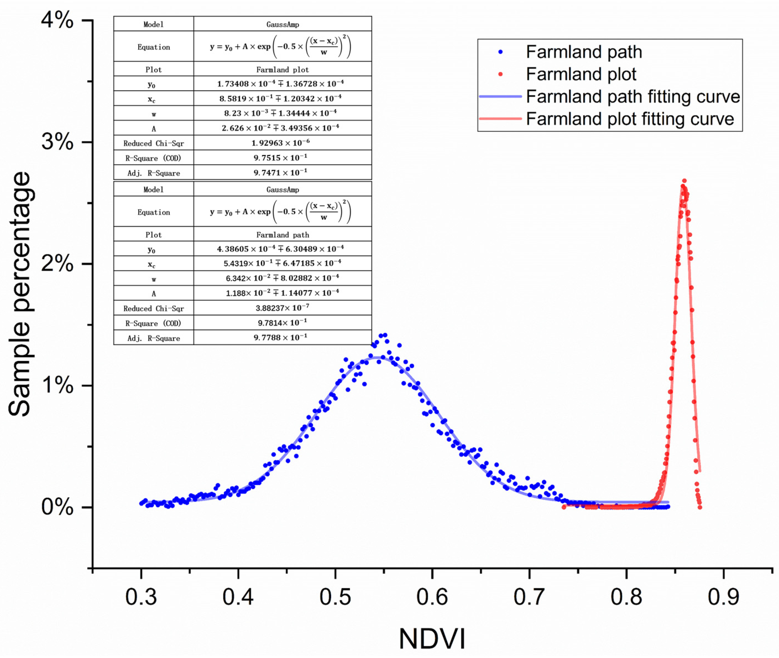
In this study, 200 samples were collected for both farmland plots and farmland paths. The NDVI values of the sample areas were calculated, and a discrete-point Gaussian fitting analysis was conducted for both types of samples. Based on the results, the NDVI values of the central axis of the Gaussian fitting curve for farmland path samples were significantly lower than those for farmland plots (
Figure 7). Through on-site surveys, it was discovered that the reason for this phenomenon was that the optimal time for extracting farmland plots was during the crop reproductive growth stage. At that time, farmland plots had a higher vegetation coverage, while farmland paths, although covered with some vegetation, had lower vegetation coverage when compared to farmland plots. As a result, it is possible to increase the farmland path land type in non-agricultural land class samples. Accurate extraction of farmland paths can then allow for the segmentation of large contiguous farmland into individual plots.
To prevent overfitting during the training process, sample selection should ensure a spatially uniform distribution across the study area, with the number of samples determined based on the proportions of different land cover types within the region.
3.5. SVM Classification Algorithm
In practical applications, the selection of classification algorithms needs to comprehensively consider factors such as data volume, feature selection, and computational efficiency. In this study, an object-oriented SVM classification algorithm was chosen to classify the multi-scale segmentation results for farmland plots. The reasons for selecting the SVM algorithm are as follows.
- (1)
Excellent classification performance: The SVM algorithm demonstrates outstanding performance in handling binary classification problems, such as distinguishing between farmland plots and non-farmland areas. By finding the optimal hyperplane to maximize the classification margin, the SVM effectively classifies different categories of land types.
- (2)
Ability to handle high-dimensional features: Extracting farmland plots may require considering multiple features. The SVM algorithm introduces kernel functions to map low-dimensional features into a higher-dimensional space for classification, better capturing the nonlinear relationships between features.
- (3)
Robustness to noise and outliers: The SVM algorithm robustly handles noise and outliers by maximizing the margin between classes, reducing their influence on the classification results.
- (4)
Interpretability and localization capability: The SVM algorithm produces a model that accurately identifies support vectors. Analyzing these support vectors allows for the interpretation of the decision-making process and enables the localization of farmland plots.
In summary, the object-oriented SVM classification algorithm demonstrates good adaptability and performance in the extraction of farmland plots, effectively classifying multi-scale segmentation results and enhancing the accuracy and reliability of farmland plot extraction.
The basic model of an SVM is designed to define a linear classifier with the maximum margin in the feature space. Unlike the perceptron, it seeks to solve for the separation hyperplane that can correctly divide the training dataset while maximizing the geometric margin. For linearly separable datasets, such a hyperplane is unique (
Figure 8) [
48,
49].
A training dataset in the feature space is shown in the following equation:
where
∈ Rn,
∈ (−1,1),
= 1, 2, 3, ...,
.
is the
feature vector, and
is the class label, which is positive when it equals +1 and negative when it equals −1.
The decision boundary B of a linear classifier can be represented in the following form: a hyperplane can be uniquely determined by the parameters (
,
), where
represents the normal vector of the plane and b represents the displacement vector of the plane. Therefore, the hyperplane can be represented as (
,
), and its expression is as follows:
where
is the normal vector of the plane, and
is the displacement vector of the plane.
Two parallel margin boundaries,
and
can be represented as follows, where the decision boundary and the two margin boundaries are parallel to each other, and the distance (functional margin) between each margin boundary and the decision boundary is 1. That is,
.
For a given dataset
and a hyperplane represented as
, the geometric margin of the hyperplane with respect to a sample point
is defined using the following equation:
The minimum value of the geometric margin of the hyperplane with respect to all sample points is
This distance is the distance from the support vectors to the hyperplane.
The SVM algorithm in this paper uses a 7:3 ratio of training to test set, with a maximum of 10,000 iterations and a tolerance of 0.001. In addition, this study introduces a regularization term into the SVM algorithm to constrain the optimization process, control model complexity, and prevent overfitting. The regularization parameter C is used to balance the trade-off between the classifier’s tolerance for training errors and the maximization of the margin. In this study, C is set to 2, using moderate regularization strength to effectively suppress the risk of overfitting while ensuring classification accuracy.
3.6. Normalization of the Farmland Plot Extraction Results
Multi-scale segmentation is the process of segmenting neighboring pixels with the strongest homogeneity in spectral and texture features into a polygonal object. The minimum unit of this process is a pixel, and a segmented vector is formed by connecting the boundaries of neighboring pixel grids that make up a polygonal object. However, this method can result in jagged edges in the extracted farmland plot vectors, which do not match the actual situation. Therefore, after using the SVM classification method to extract farmland plots, it is necessary to smooth the farmland plot vectors. In this study, a sample farmland plot in the test area was selected to demonstrate the comparison of the results before and after smoothing the farmland plot vectors (
Figure 9). In
Figure 9, b and c represent farmland plot vectors before and after smoothing, respectively. By comparing the results, one can observe that smoothed vector results show a significant reduction in jagged edges compared to before smoothing the vector. The smoothing principle is based on a polynomial fitting algorithm, with the specific principles outlined as follows.
First, assume there is a set of input points
, where
Pi represents a point on a two-dimensional plane. To smooth the vector representation, the average value of all points in the neighborhood of each point
needs to be calculated. Assume the neighborhood radius is
r. For each point
, calculate the average coordinates of all points within its neighborhood, denoted as
. For each point
, calculate the difference vector between itself and the average value of the neighboring points,
.
For each point
Pi, calculate its smoothed coordinates, resulting in a set of smoothed coordinate points
,
, ...,
after the process of vector smoothing.
The selection of the neighborhood radius, r, will affect the degree of smoothing. A smaller neighborhood radius will result in a stronger smoothing effect, but may also cause the loss of finer curve details, while a larger neighborhood radius may lead to over-smoothing.
4. Results and Discussion
Based on the shape and distribution of farmland plots, the plots were divided into two categories, regularly and irregularly shaped farmland plots, and these two types of farmland plots were extracted separately. To evaluate the accuracy of the extraction results, a method of randomly generating point samples (on a point-by-point basis) was used for accuracy assessment; additionally, regional-level accuracy evaluation was conducted by combining evaluation indicators such as producer, user, and overall classification accuracy. Finally, a detailed discussion and analysis of the extraction results is provided.
4.1. Extraction Results and Analysis of Regularly Shaped Farmland Plots
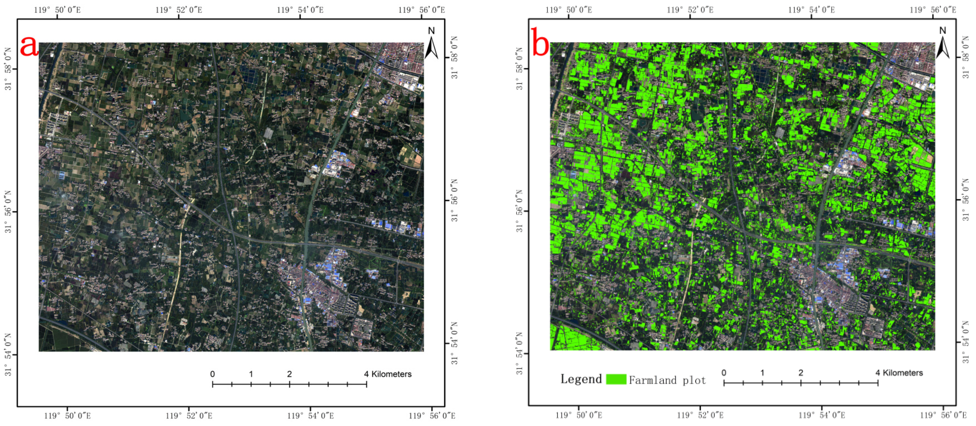
Field surveys revealed that the local government of Jintan District has taken measures to integrate fragmented farmland plots to improve the quality of arable land. The majority of fragmented farmland plots have been reorganized into larger rectangular or trapezoidal plots with regular shapes. As a result, farmland plots in Jintan are predominantly distributed in the form of a pattern of regularly shaped plots. Furthermore, asphalt roads have been constructed between some of the integrated farmland plots; these roads exhibit distinct spectral differences from the surrounding vegetation. This facilitated the extraction of farmland plots in satellite images, with the use of fewer spectral bands but with higher spatial resolution. For farmland plots without asphalt roads, the characteristic of lower vegetation cover on farmland paths compared to the vegetation cover of farmland plots can be leveraged. High-resolution images can be used, and extraction can be based on the characteristics of crop growth stages.
Based on the above approach, Jintan was taken as the study area for the extraction of regularly shaped farmland plots. A satellite image covering 100 km
2 of the study area was selected as the experimental image (RGB: 4, 3, 2) for the extraction of farmland plots, and the experimental results were obtained (
Figure 10).
For the extraction of farmland plots from the Gaofen-2 remote sensing images, it was observed that the boundaries of most farmland plots extracted were relatively complete. There were instances of misidentification and omission in small areas. Due to the research area being 100 square kilometers and classified as a medium-sized study area, selecting 50–100 sample points for each category is sufficient. To ensure the reliability of the accuracy evaluation results, this study randomly selected 300 sample points for evaluation [
50]. The accuracy of extracting regularly shaped farmland plots was relatively high, with an overall classification accuracy reaching 0.94 (
Table 2).
4.2. Extraction Results and Analysis of Irregularly Shaped Farmland Plots
Through on-site investigations, farmland plots in Xinbei District were found to be relatively small and fragmented in distribution. By using high-resolution images and extracting farmland boundaries based on the characteristics of crop growth stages, the low vegetation cover of farmland paths can be compared to that of farmland plots; this information can then be used to differentiate between the two.
Based on the above research approach, this study used Xinbei as the study area for the extraction of irregularly shaped farmland plots. A satellite image covering 100 km
2 of the study area was selected as the experimental image (RGB: 4, 3, 2) for the extraction of farmland plots, and the experimental results were obtained (
Figure 11).
The extraction of farmland plots from the Gaofen-2 remote sensing images revealed that, based on observations of the extraction results, some farmland plot boundaries were relatively complete, but there were instances of small areas of farmland plots being missed. For the given size of the study area, this study randomly generated 300 random sample points and assigned attributes to the sample points using visual interpretation. The extraction accuracy of irregularly shaped farmland plots was found to be lower than that of regularly shaped farmland plots, with an overall classification accuracy of 0.84 (
Table 3).
To improve the accuracy of extracting irregularly shaped farmland plots, this study made improvements to the original experimental scheme for extracting irregularly shaped farmland plots. The improved scheme increased the sample size of farmland plots from 10% to 30% on top of the original plan. Subsequently, another experiment was conducted for the extraction of farmland plots from the satellite image, covering 100 km
2 of the experimental area (RGB: 4, 3, 2), and the experimental results were again obtained (
Figure 12).
The experimental results were evaluated using the same accuracy evaluation sample points and method, yielding an overall classification accuracy of 0.86 (
Table 4). Compared to the original experimental results, there was a 0.02 increase in the overall classification accuracy. The user accuracy was 0.84, which is 0.08 higher than the original experimental result. Thus, increasing the sample size can slightly improve the accuracy of farmland plot extraction.
4.3. The Feasibility Discussion of Farmland Parcel Extraction Algorithm
The farmland area in southern China is relatively small, and the shapes of the plots are complex and varied, which poses challenges for farmland extraction and presents significant difficulties for modern agricultural management. This study combines crop phenological information with multi-scale classification algorithms and SVM algorithms to develop a farmland parcel extraction algorithm.
In this section, we will discuss the method, which is divided into the following three parts: first, we will introduce the feasibility of the algorithm; second, we will analyze its limitations; and finally, we will look forward to future research.
4.3.1. Feasibility of the Algorithm
This study combines crop phenological information with multi-scale classification algorithms and SVM algorithms to develop a farmland plot extraction algorithm, which offers three major advantages. First, by incorporating crop phenological information, the algorithm effectively enhances the spectral differences between farmland and non-farmland areas, laying a solid foundation for the accurate extraction of farmland plots by subsequent multi-scale segmentation algorithms. Second, the algorithm uses an object-oriented multi-scale segmentation technique, effectively overcoming common salt-and-pepper noise issues in current pixel-level classification methods, such as random forests and FCNs. The multi-scale segmentation algorithm can balance noise and boundary information at different scales, reducing noise interference, and, especially in complex backgrounds or environments with different farmland types, can more stably and completely extract the farmland boundaries. Third, by integrating the SVM algorithm, the algorithm effectively overcomes the dependency on large samples found in models like EfficientNet and VGGNet.
This study tested the feasibility and accuracy of the algorithm for the following two types of agricultural plots: regular and irregular. The test results indicate that the algorithm’s accuracy remains stable, at over 86%, with the accuracy for regular agricultural plots reaching up to 94%. The farmland plot algorithm not only effectively reduces survey costs, but also significantly improves plot management efficiency. Through automated image recognition and data analysis, agricultural managers can obtain detailed information about the farmland in real-time, avoiding the time and labor waste of traditional manual surveys.
In addition, the algorithm is integrated into an agricultural mapping system platform to achieve rapid collection and visualization of vector data of farmland plots. At the same time, it integrates soil, climate, and historical production data, providing precise guidance for agricultural management decisions. Farmers can promptly identify potential problems and take effective measures, thereby significantly improving management accuracy and response speed, and promoting the transformation of agricultural production towards modernization and intelligence.
4.3.2. Limitations of Algorithms
In this study, we propose a farmland extraction algorithm that incorporates crop phenological information, combining multi-scale segmentation with the support vector machine (SVM) algorithm. However, due to the large volume of high-resolution image data from the Gaofen-2 satellite, processing a single scene image using the multi-scale segmentation algorithm takes approximately 2 h on a computer with a CPU: AMD Ryzen 7 5800 8-core processor, GPU: NVIDIA GeForce RTX 3060, and 128 GB (2400 MHz) of RAM. As a result, the algorithm requires more computing power, including Central Processing Units (CPU) and Graphics Processing Units (GPU). To improve the algorithm’s performance, optimization strategies such as tile-based processing will be adopted in the future [
51].
4.3.3. Future Research
Future research should be based on field data to explore the issue of crop identification in agricultural plots in greater depth. With the rapid development of remote sensing technology and artificial intelligence, accurately and efficiently identifying and classifying crop types in agricultural fields has become one of the key challenges in precision agriculture management and modern agricultural development. Research can combine high-resolution remote sensing imagery data with spatiotemporal information, integrating multispectral and multi-temporal data to improve the accuracy and timeliness of crop identification. Such research will provide more precise data support for agricultural production, promote the rational allocation of agricultural resources, enhance the level of intelligent field management, and thus foster sustainable agricultural development.
5. Conclusions
This study selected the districts of Xinbei and Jintan in Changzhou City, China, as the study areas. A Gaofen-2 image covering an area of 100 km2 was used as the experimental area. This paper has proposed an object-oriented method for extracting farmland plots from high-resolution images. This method uses textural, spectral, and phenological information of crops in farmland plots to determine the optimal extraction time and segmentation scale for farmland plots. It combines on-site survey information to classify samples for farmland plot extraction. While using this method, tests and accuracy evaluations for farmland plot extraction were conducted in the two study areas, exploring the potential of farmland plot extraction under different conditions. The research yielded the following conclusions.
- (1)
In the selection of image time, the time was divided into planting and non-planting seasons based on the growth of plants in farmland plots. During the planting season, the phenological stages of crops were further categorized into the vegetative and reproductive growth stages. The multi-scale segmentation results showed that the integrity of farmland plot segmentation in non-planting season images was relatively poor. However, during the planting season, the images of crops in the vegetative growth stage exhibited better integrity in farmland plot segmentation than those in the reproductive growth stage.
- (2)
During the selection of multi-scale segmentation parameters, the segmentation parameters for object-oriented multi-scale segmentation of farmland plots were determined; these were based on the textural and spectral information of farmland plots. Among these parameters, when the segmentation scale, shape parameter, and compactness parameter were set to 59, 0.2, and 0.6, respectively, the best segmentation results were achieved.
- (3)
In the selection of the sample set, the sample types were divided into farmland and non-farmland plots. For the extraction of farmland plots in block units, it is necessary to add a category for farmland paths in the non-farmland plot types.
- (4)
In terms of farmland plot types, to improve the accuracy of farmland plot extraction, regularly and irregularly shaped farmland plots were distinguished based on the distribution type of farmland plots in each case and extracted separately. For irregularly shaped farmland plots, the sample size was increased to enhance the extraction accuracy, thereby improving the overall accuracy of farmland plot extraction.
Based on the above conclusions, this algorithm integrates crop phenological information and demonstrates exceptional accuracy in farmland parcel recognition. It is applicable to multiple agricultural fields, especially in the digitalization of parcel boundaries in high-standard farmland construction and the area verification in agricultural subsidy distribution. In the process of high-standard farmland construction, the algorithm can accurately identify and delineate land boundaries, improving the precision and efficiency of parcel planning. In agricultural subsidy distribution, the algorithm helps governments and relevant departments to accurately verify the actual area of each farmland, ensuring the fairness and transparency of subsidy allocation while effectively reducing the possibility of human error.
However, this study has limitations, in that it only involved research into the extraction of farmland plots from high-resolution images, without further identifying the crops within the farmland plots. Therefore, the authors plan to focus on studying methods for identifying crops in farmland plots in their subsequent research, providing important technical support for services such as crop management, growth monitoring, and yield estimation in the field of green agriculture. This will further promote the sustainable development of green agriculture.


