Artificial Intelligence Models for Bankruptcy Prediction in Agriculture: Comparing the Performance of Artificial Neural Networks and Decision Trees

Abstract

Debt levels are a crucial factor when assessing the financial stability of agricultural firms, and excessive indebtedness is usually the most important indicator of financial distress. As agriculture is a capital-intensive sector with a high reliance on borrowed funds, firms in this sector are more vulnerable to insolvency. This study examines the performance of artificial neural networks (ANNs) and decision trees (DTs) in predicting the bankruptcy of Slovak agricultural enterprises. In an attempt to compare the models’ performances, the most consequential indebtedness ratios are investigated through machine learning approaches. ANN and DT models are found to perform significantly better than traditional forecast methods. ANN achieved an AUC of 0.9500, accuracy of 96.37%, precision of 96.60%, recall of 99.68%, and an F1-score of 98.12%, determining its robust predictive ability. DT performed a little better on AUC (0.9550) and achieved an accuracy of 97.78%, precision of 98.69%, recall of 99.01%, and an F1-score of 98.85%, determining its predictive ability and interpretability. These findings confirm the potential for applying AI-based models to enhance financial risk assessment. This study provides informative results for financial analysts, policymakers, and corporate managers in support of early intervention strategies. Additional research would be required to explore state-of-the-art AI techniques to further refine bankruptcy forecasting and financial decision-making in vulnerable sectors like agriculture.

1. Introduction

Recently, the rapid development of artificial intelligence (AI) has significantly influenced numerous sectors, including finance, healthcare, manufacturing, and agriculture [1,2,3]. AI-driven methods offer complex instruments with the capabilities of dealing with high-level, non-linear relationships among data and thus are best suited for uses such as risk assessment, fraud detection, and financial forecasting [4,5,6]. Of the AI techniques, artificial neural networks (ANNs) and decision trees (DTs) are some of the most widely used machine learning models in corporate bankruptcy forecasting. Their popularity is because they can process large datasets, find hidden patterns, and predict more accurately and quickly than traditional statistical techniques. With their multi-layered structure, ANN models are better at simulating complex interactions between variables. On the contrary, DT models are better for helping decision-makers figure out why enterprises are having financial problems because they are easy to understand. The growing popularity of machine learning models for bankruptcy prediction is a testament to the weaknesses inherent in earlier methods such as discriminant analysis and logistic regression. Traditional models tend to presuppose linear relationships and impose rigid statistical requirements, such as homoscedasticity and normality of residuals, which cannot be satisfied in practical situations where economic information tends to be noisy, unbalanced, and subject to many external influences [7,8]. In addition, AI models like ANN and DT are more generalizable and flexible in that they can generalize well and achieve more accurate classification even when handling complicated and diverse datasets [9,10]. Such models, therefore, have been drawing increasing interest in studies and actual applications concerning early warning systems of bankruptcy prediction.

Despite significant progress in this field, the issue of financial distress and bankruptcy prediction remains uninvestigated in certain sectors [11], primarily agriculture, and in developing nations such as Slovakia. The agricultural sector is of crucial significance to the Slovak economy, providing primary raw materials for manufacturing industries such as food production, textiles, construction, and energy. Moreover, it is a primary force behind rural development, conservation of biodiversity, and environmental sustainability. Nevertheless, Slovak agricultural companies are prone to numerous factors that render them more susceptible to financial turmoil and insolvency. These factors include commodity price volatility, dependence on climatic factors, market volatility, and dependency on government subsidies and foreign trade policies. Agricultural firms have high operating expenses, long production cycles, and liquidity shortages, which are more prone to financial distress than other businesses. Additionally, inefficiencies in managing long-term debt commitments and extrinsic fluctuations are likely to increase their financial vulnerability. These characteristics highlight the urgent need for effective bankruptcy forecasting models tailored to the specific needs of the agricultural sector. Such models can provide initial signals of potential financial problems so that stakeholders may take preventative actions and implement strategies to mitigate the risk of insolvency [12].

The higher vulnerability of agricultural enterprises in Central and Eastern Europe, particularly in Slovakia, requires building sound early warning systems that recognize financial distress before reaching the point of insolvency. The agriculture sector is exposed to highly distinctive conditions, including seasonality patterns in revenues, subsidy reliance, and capital intensity, which distinguish it from other sectors and render financial risk difficult to evaluate. In such an environment, traditional statistical models relying on linearity and normality assumptions will at times fall short or even be misleading, which has prompted researchers to look for alternative methods that can detect non-linear relationships and complex patterns in financial data. This study seeks to address a several of crucial research questions:

• RQ1: Do ANNs outperform DTs in predicting bankruptcy of agricultural firms in terms of classification accuracy and area under the curve?
• RQ2: To what extent can DT models enhance interpretability in bankruptcy prediction compared to ANN models, particularly in terms of transparent decision rules and threshold identification?
• RQ3: Which financial indicators most strongly influence the classification of firm solvency or insolvency?

The main aim of this paper is to develop a predictive model for identifying financial distress and bankruptcy threats in Slovak agricultural companies through ANN and DT models. Since the industry is vulnerable to economic crises, i.e., excessive borrowing and financial instability, the present research tries to explore the most significant determinants causing the financial issues of agricultural firms. These models are now being employed to predict bankruptcies across various industries because they can handle complex, non-linear interrelations between financial variables. Under agriculture, this study seeks to determine and analyze the key drivers of financial distress, such as indicators of indebtedness, to better understand the factors contributing to the risk of bankruptcy. The research begins with the application of statistical tests, i.e., Levene’s test and the t-test, to verify the homogeneity of variances and whether some financial variables are significant. These predictive models are then developed using ANN and DT methods since these are capable of suitably addressing the nature of the complexity involved in the data. To measure the performance and efficacy of such models, measures such as the area under the curve, accuracy rate, and F1-score are utilized. While there exists a significant literature on predicting bankruptcy across industries, research on the agricultural industry is not as frequent. The current literature tends to emphasize agricultural firms’ distress by emphasizing the unique characteristics of this industry, such as the impact of climatic risks, market volatility, and the structural challenges of family-owned firms, which are predominant in agriculture. Despite the crucial contribution of this sector, there exists a notable gap in the literature in terms of research on forecasting bankruptcy for agricultural companies, particularly through the use of advanced AI techniques such as ANN and DT. The present study attempts to bridge this gap by exploring the feasibility of these machine learning algorithms in bankruptcy prediction in the Slovak agricultural sector. In so doing, it helps to make early warning systems stronger that can be utilized for making decision-making processes, strengthening financial stability and ensuring the long-term sustainability of agricultural businesses.

This study bridges the gap in accurate and interpretable sector-specific models for agricultural company bankruptcy prediction through AI approaches. Specifically, it compares two data-driven techniques to establish their feasibility in predicting insolvency among Slovak agricultural enterprises. This research is motivated by a need to provide stakeholders with improved predictive tools that not only are more accurate in their prediction, but also yield insight into the financial indicators most responsible for distress. By integrating machine learning techniques with the domain of agricultural financial analysis, this research aims to contribute to both the academic literature on AI in finance and the operational needs of financial decision-making. Methodological design encompasses stratified sampling to achieve balanced representation, statistical testing for preselecting proper indicators, and model performance comparison. By this, this research seeks to answer the question posed above and lay the groundwork for subsequent predictive modeling endeavors in the industry. The research’s findings are to be applied in informing policy, guiding future model design, and ultimately enhancing agricultural financial resilience.

This paper is divided into the following sections. The literature review in Section 2 aims to review the available knowledge of bankruptcy and indebtedness in the agriculture sector, focusing on key financial indicators that cause financial distress and methodologies applied to predict such incidences. The methodology presented in Section 3 provides information on the study design, sources of data, and statistical analyses applied in this study. It describes how data were extracted from the ORBIS database, the qualitative parameters in the choice of agricultural firms, and the rationale behind using ANN and DT for the bankruptcy prediction model. In the results and discussion, presented in Section 4 and Section 5, respectively, the outputs of the bankruptcy prediction model developed using ANN and DT are compared with the existing literature. The debate concerns how the results contribute to previous research on the financial problems of agricultural firms. The prediction models are then examined in light of the peculiarities of the Slovak agricultural economy, assessing how effectively they might identify the potential risk of bankruptcy. Finally, the conclusions, presented in Section 6, discuss the implications of the study for policymakers, financial institutions, and entrepreneurs and hint at future directions of research, such as exploring additional financial and non-financial indicators that can influence the debt organization and risk of bankruptcy of agricultural firms.

2. Literature Review

Over the years, many approaches have been developed to predict corporate bankruptcy, beginning with traditional statistical methods like discriminant analysis and logistic regression [13,14,15]. These early models laid the groundwork for financial distress measurement based on the study of significant financial ratios, presenting relatively simple yet effective forecasting models. In subsequent decades, new methods emerged, including decision tree algorithms [16,17], genetic algorithms [18,19,20], support vector machines [21,22,23], and random forests [24,25,26]. Comparative studies have been increasingly interested in examining the performance of such machine-learning approaches in improving bankruptcy prediction accuracy [27,28,29].

Since the 1990s, with the advent of artificial intelligence algorithms, there has been widespread use of ANN models, and these went on to become a very popular machine learning technique for forecasting financial distress [30,31,32]. While ANNs have continued on robust prediction paths at all times, there is now growing interest in deep learning models. These advanced methods circumvent the main drawbacks of traditional neural networks, such as the vanishing gradient issue, overfitting, and high computational demands, by employing architectures with the potential to have several hidden layers and improved optimization methods [33,34].

Corporate bankruptcy prediction has been a critical domain of financial research in recent decades, and greater interest in using machine learning algorithms has developed over time. Out of them, ANN and DT models have emerged as being popular because they have the capability of dealing with non-linear relationships of complex financial variables and the risk of bankruptcy. Initial studies, for instance, Swicegood and Clark [35], compared ANN models with discriminant analysis and expert judgment, and reported marginally better performance of ANN in predicting non-prosperous banks. Akkaya et al. [36] tested the capability of ANN models by forecasting financial failure in Turkish firms with 81% accuracy. The same results were obtained by Lacher et al. [37], Etheridge et al. [38], and Bloom [39], who all demonstrated the effectiveness of ANN models in distinguishing prosperous and non-prosperous firms. Le and Viviani [40] also emphasized the forecasting advantage of ANN and k-nearest neighbor (kNN) models over conventional models when examining 3000 American banks, and showed that ANN can outperform SVM in forecasting financial distress in the Turkish industry. With the continuously superior predictive performance of ANN models across various financial environments, the following is hypothesized:

H1: 

ANN will achieve significantly higher predictive performance than DT in terms of area under the curve and overall classification accuracy.

Several research studies have also sought to improve ANN models by integrating metaheuristic algorithms. Pendharkar and Rodger [41] used genetic algorithms to update the weights of ANN, while Zhang et al. [42] introduced hybrid PSO-BP methods that paired particle swarm optimization (PSO) with backpropagation. Sarangi et al. [43] further developed this research by presenting a differential evolution–backpropagation (DE-BP) model that enhances feedforward neural network training. Such methods overcome limitations in traditional backpropagation algorithms and improve classification accuracy, Blum and Roli [44] assert.

In terms of DT implementations, while considered less accurate than ANN, DT models are easier to interpret and thus useful for stakeholders who want decision-making to be transparent. Shafiee et al. [45] demonstrated that support vector machines (SVMs) were superior to DT and ANN models in the classification of bankrupt companies on the Tehran Stock Exchange. Ptak-Chmielewska [46] also found that SVM was superior to linear discriminant analysis (LDA) in Poland. Thilakaratna et al. [47] utilized a deep neural network (DNN) with new financial ratios, having high prediction capability for UK and Irish firms.

Consistent across these studies is the result that primary financial ratios are powerful predictors of bankruptcy. Pendharkar [48] and Korol [49] emphasized the debt-to-equity ratio and liquidity indicators in their ANN models. Behr and Weinblat [50] confirmed their relevance using random forest methods for various European nations. Mihalovic [51] and Horvathova et al. [52] also chose the debt-to-equity ratio as a dominant predictor in Slovak companies, where ANN models provided higher classification accuracy than traditional methods. Tudor et al. [53] also confirmed the significance of the interest coverage ratio and financial independence ratio in Romanian firms through DT methodologies aligned with the result of this research, wherein such ratios were confirmed to have high predictive power. Korol [54] further emphasized profitability and liquidity as key drivers for ANN bankruptcy prediction, a contention reinforced by Radovanovic and Haas [55], who found leverage and liquidity ratios superior to other financial metrics. Chen [56] focused on how the financial independence ratio is crucial for Taiwan, on the heels of DT model outputs that assigned to it a value of high importance. Jeong et al. [57] demonstrated the usefulness of interest burden and cash flow-to-debt ratios in establishing the ability of the firm to generate cash flow to repay its debts; however, this was less emphasized in research by Mihalovic [51], where profitability and leverage ratios were accorded higher preference. As leverage and liquidity ratios have been shown to be very good predictors in previous studies on different models, the following hypothesis is:

H2: 

Leverage and liquidity-related financial indicators (e.g., debt-to-equity ratio, financial independence ratio) will have the highest importance scores in both ANN and DT models.

Advanced machine learning models have proven to be very effective across various domains and nations. ANN models have also been compelling in terms of predictive accuracy. Pamuk et al. [58] and Shetty et al. [59] both achieved more than 82% accuracy with just five variables. Radovanovic and Haas [55] and Ben Jabeur and Serret [60] also achieved good accuracy with ANN models, indicating that they can understand complex financial information. Kuiziniene and Krilavicius [61] improved ANN model performance to 92% accuracy by applying SMOTE to resample datasets, while Hamdi et al. [62] achieved nearly 98% accuracy using a DNN model for Tunisian firms. Chen et al. [63] demonstrated the potential of hybrid ANN models based on genetic algorithms and fuzzy logic, achieving an AUC of 0.979 and an accuracy of over 96% in Taiwan’s electronics sector.

While ANN models are more effective in predictive accuracy than DT models, the latter are useful because they are interpretable. Pamuk et al. [58] and Shetty et al. [59] set the same levels of accuracy for ANN and DT models. Radovanovic and Haas [55] and Ben Jabeur and Serret [60] also documented the same performances for both methods. Kuiziniene and Krilavicius [61] reported slightly lower accuracy for DT compared to ANN, but Fasano et al. [64] argued that the loss in accuracy was justified by DT’s increased transparency. Njoku et al. [65] demonstrated how the ensembling technique with DT could also improve prediction accuracy to 88.5%. Garcia [66] noted that the number of predictors used in a model does not necessarily relate to its accuracy. Due to the transparent, rule-based nature of decision tree architecture, especially compared to the “black-box” nature of ANN, the third hypothesis is advanced:

H3: 

DT models will demonstrate significantly greater interpretability than ANN models, as evidenced by the clarity of decision thresholds and model structure.

In Slovakia, several studies have established the effectiveness of machine learning methods for bankruptcy prediction. Mihalovic [51] found that DT was more effective than traditional statistical approaches, with an accuracy rate of 83.5%, whereas Horvathova and Mokrisova [67] emphasized the need for advanced algorithms like ANN and DT to detect complex, non-linear patterns in financial data. Durica et al. [68] confirmed ANN’s improved performance over DT in Slovak firms, with AUC values over 0.90. Horvathova et al. [52] applied ANN and DT models to Slovak construction firms, noticing ANN’s high accuracy but recognizing DT’s transparency. Letkovsky et al. [69] achieved a 92% accuracy rate in bankruptcy prediction using an ANN model, noticing its ability to identify complex financial interdependencies. Gavurova et al. [70] carried out this analysis for the Slovak automotive and engineering industries, using an ANN model and logistic regression on five years of data from 2384 firms. Their ANN model showed great performance with an accuracy rate of 93.53%, verifying ANN’s utility in predicting early bankruptcy risk. Moreover, Jencova et al. [71] developed an early warning system for Slovak non-financial corporations using an ANN model and achieved an 86.7% accuracy rate, validating the role of ANN in improving financial decision-making in Slovakia.

Although ANN and DT models have become popular for predicting bankruptcy because of their predictive accuracy and versatility in application, they still face constraints regarding interpretability. Linear and logistic regression model formulations, if less accurate regarding non-linear estimation, provide explicit insight into effect direction (positive or negative) and degree through model coefficients. This aspect is generally significant when decision-makers seek to understand causality rather than classification. Moreover, ensemble models such as random forests provide an exciting balance between accuracy and interpretability, as they aggregate numerous decision trees to reduce variance and overfitting but still permit users to explore variable importance scores. However, RF was not implemented within this study due to the relatively small sample size and the need to compare two established methods, while it remains a useful method for continuing bankruptcy prediction studies in agriculture in the future, especially as larger datasets become available.

While machine learning models are common in bankruptcy prediction, none directly address the agricultural sector, even in Slovakia or comparable economies. Most of the available models relate to manufacturing, banking, or general small and medium-sized enterprises (SMEs), and are not tuned to the financial characteristics of agricultural enterprises, such as high seasonality, dependence on subsidies, and asset illiquidity. Moreover, comparative performance and interpretability trade-offs between DT and ANN have not been properly studied under these circumstances. By subjecting formulated hypotheses to tests, this research aims to make a contribution not only to the understanding of model performance, but also to the understanding of the financial characteristics most highly linked with distress in the agricultural sector, which eventually assists in building more targeted and interpretable early warning systems more appropriate to sectoral needs.

3. Methodology

The main aim of this paper is to develop a predictive model for recognizing financial distress in Slovak agricultural companies via the use of ANN and DT models. Since the economy is facing challenges in the agricultural sector, particularly financial instability and increased indebtedness, the identification of determinants propelling financial difficulties has gained further significance. By utilizing advanced machine learning techniques such as ANN and DT, this research seeks to provide valuable insights into the financial health of agricultural enterprises. The model will be capable of pinpointing key drivers of risk and providing early warning signals of possible financial distress, resulting in more informed decision-making and strategic planning for industry players.

Data for the development of a bankruptcy prediction model for Slovak enterprises operating in the agricultural sector came from the ORBIS database, a business and finance information source on more than 400 million public and private companies operating all over the world. The information on financial indicators used to model bankruptcy consisted of data on 2095 agri-business companies operating in Slovakia in 2022 (for all independent variables, i.e., individual financial indicators) and in 2023 (for the dependent variable, i.e., business stability). Agricultural enterprises were selected using the NACE classification system, that is, by selecting all the units classified in Section A (Agriculture, Forestry and Fishing), divisions 01 (Crop and animal production, hunting, and related service activities), 02 (Forestry and logging), and 03 (Fishing and aquaculture). This wide selection covers a wide range of operations, such as the growing of non-perennial and perennial crops, animal breeding, mixed farming, ancillary services, silviculture, logging, and freshwater and marine fishing and aquaculture. However, because it was not appropriate to estimate financial indicators for some of the companies in practice, the information taken from the database was consequently modified. Firms that were unable to provide all the input data to be used for the computation of the key mathematical formula during the observation period were excluded from the dataset, reducing the reporting ability of the results collected. Financial variables are normally utilized as explanatory predictors by Andresson and Lukason [72] when dealing with bankruptcy models. These measures normally have the propensity to provide an asymmetric distribution as they contain outliers. The literature employs various ad hoc techniques to identify and correct extreme values without outliers. However, the impact of these techniques on model predictive accuracy is unknown. While there is agreement in the literature that outliers must be corrected, it is unknown which values are extreme and must be corrected to maximize model predictive capability. For this purpose, the dataset was subjected to the removal of its outlier values to enhance the informativeness of the resultant outcomes from the calculated debt analysis based on the Z-score method. The application of this process makes it possible to assess the difference between each received signal strength observation and the time-series mean received signal strength observation. Subsequently, the outcome is divided by the observation’s standard deviation. A Z-score of 0 means that the mean of the received signal strength observation and the time-series observation are the same. Positive and negative Z-scores indicate that the received signal strength measurement is above and below the mean, respectively. A received signal strength observation is considered an outlier if the value of its Z-score exceeds a pre-set threshold. Typically, the most commonly used threshold in outlier detection is ±3, as stated by Yaro et al. [73]. Thus, in this research paper, any received signal strength observation with a Z-score value greater than ±3 was considered an outlier. After the final set of corrections (deletion of unavailable and outlying values), the dataset consisted of 1123 enterprises involved in the agriculture sector that used the prediction model. For model training and testing, the final dataset was divided randomly into two subsets: 70% for training and 30% for testing. Stratified sampling was applied to preserve the small subset of distressed firms proportionally in both subsets to avoid any class imbalance bias of the dataset.

Accurate identification of corporate financial well-being and good predictors of financial performance must be well established. In bankruptcy prediction, conventional and, to a certain degree, multidimensional discriminant analysis or Z-score analysis, classifies the companies based on financial variables and cannot accurately depict the theory behind the nature of the non-linear relationship among such variables. ANN and DT models do have an advantage over some others in modeling these complex, inter-variable interactional relationships. While discriminant analysis is based on linear combinations of variables, ANNs have the intrinsic capability to discern hidden relationships among data. ANNs are thus applied to predict bankruptcy because they would bring to the surface or demonstrate some of the hidden relationships that could escape normal detection.

When the indicators highlighted by prominent researchers [14,15,69,74,75,76,77,78] are aimed at, determination of the independent variables employed in the construction of the model as the most important determinants of financial health is required. The selected debt indicators and the interdependencies needed to calculate them are outlined in

Table 1. Summarized formulas of financial indicators.

Input Neuron	Indicator	Algorithm	Input Neuron	Indicator	Algorithm
TI	Total indebtedness ratio	${\displaystyle \frac{\mathrm{NCLI}+\mathrm{CULI}}{\mathrm{TOAS}}}$	IB	Interest burden ratio	${\displaystyle \frac{\mathrm{INTE}}{\mathrm{EBIT}+\mathrm{INTE}}}$
SF	Self-financing ratio	${\displaystyle \frac{\mathrm{SHFD}}{\mathrm{TOAS}}}$	DCF	Debt-to-cash flow ratio	${\displaystyle \frac{\mathrm{NCLI}+\mathrm{CULI}}{\mathrm{EAT}+\mathrm{DEPR}}}$
CI	Current indebtedness ratio	${\displaystyle \frac{\mathrm{CULI}}{\mathrm{TOAS}}}$	FI	Financial independence ratio	${\displaystyle \frac{\mathrm{SHFD}}{\mathrm{NCLI}+\mathrm{CULI}}}$
NCI	Non-current indebtedness ratio	${\displaystyle \frac{\mathrm{NCLI}}{\mathrm{TOAS}}}$	EL	Equity leverage ratio	${\displaystyle \frac{\mathrm{TOAS}}{\mathrm{SHFD}}}$
DE	Debt-to-equity ratio	${\displaystyle \frac{\mathrm{NCLI}+\mathrm{CULI}}{\mathrm{SHFD}}}$	NCAC	Non-current assets coverage ratio	${\displaystyle \frac{\mathrm{SHFD}+\mathrm{NCLI}}{\mathrm{FIAS}}}$
IC	Interest coverage ratio	${\displaystyle \frac{\mathrm{EBIT}}{\mathrm{INTE}}}$	Ins	Insolvency ratio	${\displaystyle \frac{\mathrm{NCLI}+\mathrm{CULI}}{\mathrm{DEBT}+\mathrm{OCAS}}}$

Note: NCLI Non-Current Liabilities, CULI Current Liabilities, TOAS Total Assets, FIAS Fixed Assets, SHFD Shareholders Funds, EBIT Earnings Before Interest and Taxes, INTE Interest Paid, EAT Earnings After Taxes, DEPR Depreciation and Amortization, DEBT Debtors, OCAS Other Current Assets. Source: Valaskova et al. [79].

.

The total indebtedness ratio expresses the proportion of debt in the total assets of enterprises. Optimum indebtedness guarantees the reduction in the cost of capital and, consequently, maximizes the firm’s market value. The target value in developed market economies ranges from 70 to 80% [80], and in other economies, between 30 and 60% [81]. The complement to the total indebtedness is the self-financing ratio, which reflects the extent to which a firm finances its asset needs through shareholders’ funds, which is quantified as the ratio of equity to total assets [82], and its value must not fall below 20–30% [79]. If an enterprise predominantly relies on debt financing, it is necessary to more deeply examine the debt structure through partial financial structure indicators. The current indebtedness ratio expresses the ratio of short-term obligations to total assets and demonstrates the company’s capability to settle obligations falling due within one year. The higher the value, the more pressure on liquidity [83]. The non-current indebtedness ratio expresses the percentage of long-term liabilities to total assets. It indicates the firm’s long-term financial stability, particularly concerning obligations of more than one year’s maturity [84]. The debt-to-equity ratio conveys the relationship of total debt to equity and serves the same purpose as the total indebtedness ratio. A ratio that is higher indicates high risk for the creditors. A ratio near 1 (or 100%) is considered balanced, as it suggests that there is sufficient equity to cover all liabilities [79]. The interest coverage ratio faces off EBIT and interest expenses. The lower this ratio, the more burdensome are interest expenses. The indicator shows how many times a firm can pay interest costs with earnings. Even though an optimum is 5, the key is not to fall below 3 [85]. The interest burden ratio is the opposite of interest coverage and is the percentage of interest expenses to operating profit. It needs to be below 100% because its high value may reflect that although there is sufficient profit available for interest coverage, the enterprise may not be efficiently using its debt [86]. The debt-to-cash flow ratio computes the firm’s ability to service debt using internal cash flow and indicates the number of years needed to settle debts. The optimum is a figure between 3 and 4, and a negative value is a sign of the inability to service debts [79,87]. The financial independence ratio measures the firm’s reliance on internal versus external funding. A larger number expresses greater financial independence and less bankruptcy risk, while a smaller number suggests dependence on indebtedness and higher vulnerability. The equity leverage ratio evaluates the mix of debt and equity used in the financing of business activities. A general ideal figure is around 4, which implies that 75% of company activities are financed through debt [86]. The non-current assets coverage ratio reflects the extent to which long-term resources cover non-current assets, where a value above 1 indicates overcapitalization and a preference for long-term solvency and stability over short-term gains. The insolvency ratio relativizes liabilities and receivables. A ratio of more than 1 suggests primary insolvency, in which liabilities surpass receivables and are the result of internal weakness. In contrast, a ratio of less than 1 points to secondary insolvency, in which unpaid customer receivables mean the company cannot pay its obligations [79].

The individual enterprises used in the prediction model should be classified into two relevant groups. The first group is made up of successful companies with an acceptable level of debt and no significant financial difficulties. However, the second group consists of companies with a higher level of debt that also experience financial issues. Generally, the basis on which the models are grounded is the performance of a non-prosperous company, based on which a firm has financial difficulties if its equity-debt ratio, which measures a diminishing position of financial independence and firm creditworthiness, is less than 0.08. If the equity-to-debt ratio is less than this, the indebtedness level is not rational, and the firm is in crisis. The limit value of the debt-to-equity ratio is determined statutorily by the Slovak Commercial Code, and it must be monitored in order not to let the firm fall into bankruptcy, as the crisis management of the enterprise was the foundation for model development [88]. The estimated output Y can be expressed as binary values:

$$Y=\left\{\begin{array}{c} 0 for non-properous firm\\ 1 for prosperous firm\end{array}\right.$$

(1)

Based on this classification criterion, the data required for the construct models based on ANN as well as DT includes information regarding 1069 performing businesses and 54 non-performing businesses.

1. For the development of the prediction models, some initial processing steps are necessary with the analysis. Firstly, it is necessary to reduce the dimensionality of the original dataset, i.e., the dimensionality of the learning set, by selecting the optimal appropriate ratios for the prediction of bankruptcy. Independent sample t-tests (Student’s t-tests) are performed based on the learning set to explore whether the mean values of the ratio of the two groups, i.e., from the prosperous and non-prosperous firms, differ statistically. In case a statistical difference exists among the means of the two groups, then the ratio will be used in the prediction model.

Before conducting an independent samples t-test, the equal variances assumption (homogeneity of variance) must be tested across groups. According to Parra-Frutos [89], Levene’s test is applied to test the null hypothesis of equal population variances. Independence of observations and a quantitative dependent variable are the two conditions that must be met for Levene’s test. Levene’s test is essentially a one-way ANOVA on the absolute deviations from the group means $Z_{ij}=\left|Y_{ij}-{\overline{Y}}_i\right|$, where $Y_{ij}$ is the $j$-th group value, and ${\overline{Y}}_i$ is the mean of the $i$-th group [90]. The test statistic $W$ is calculated as:

$$W={\displaystyle \frac{\left(n-2\right){\sum }_{i=1}^2{N}_i{\left({\overline{Z}}_i-\overline{Z}\right)}^2}{{\sum }_{i=1}^2{\sum }_{=1}^{N_i}{N}_i{\left(Z_{ij}-{\overline{Z}}_i\right)}^2}}$$

(2)

where $N_i$ is the size of each group, $n$ is the total sample size, ${\overline{Z}}_i$ is the mean of $Z_{ij}$ within the $i$-th group, and $\overline{Z}$ is the grand mean of all $Z_{ij}$. The statistic $W$ follows an $F$-distribution with 1 and $n-2$ degrees of freedom. If $W$ exceeds the critical value $F\left(\alpha ,1,n-2\right)$, then the null hypothesis of equality of variances is rejected. In this study, $\alpha =0.05$ was used as the level of significance [91].

If Levene’s test reveals equal variances, the standard independent samples Student’s t-test is employed, where the test statistic is as follows:

$$t={\displaystyle \frac{{\overline{X}}_1-{\overline{X}}_2}{s_p\sqrt{\frac{1}{n_1}+\frac{1}{n_2}}}}$$

(3)

where ${\overline{X}}_1$ and ${\overline{X}}_2$ are the sample means, $n_1$ and $n_2$ are the sample sizes, and $s_p$ is the pooled standard deviation:

$$s_p=\sqrt{{\displaystyle \frac{\left(n_1-1\right)s_1^2+\left(n_2-1\right)s_2^2}{n_1+n_2-2}}}$$

(4)

where $s_1$ and $s_2$ are the standard deviations of each sample. Then, the test statistic value is compared with the critical $t$-value from the $t$-distribution table having degrees of freedom $df=n_1+n_2-2$ [92].

If Levene’s test indicates unequal variances, Welch’s t-test is used instead. Its test statistic is:

$$t={\displaystyle \frac{{\overline{X}}_1-{\overline{X}}_2}{\sqrt{\frac{s_1^2}{n_1}+\frac{s_2^2}{n_2}}}}$$

(5)

with the degrees of freedom calculated by the Welch–Satterthwaite equation:

$$df={\displaystyle \frac{{\left(\frac{s_1^2}{n_1}+\frac{s_2^2}{n_2}\right)}^2}{\frac{1}{n_1-1}{\left(\frac{s_1^2}{n_1}\right)}^2+\frac{1}{n_2-1}{\left(\frac{s_2^2}{n_2}\right)}^2}}$$

(6)

In either type of the t-test, the calculated t-value is compared with the t-distribution’s critical value. The null hypothesis of equal group means is rejected if the test statistic is greater than the critical value [93].

2. Following the preliminary analysis, the confirmed and pre-processed input feature dataset was employed to construct two classification models, namely an artificial neural network and a decision tree.

Artificial neural networks (ANNs) find widespread applications in statistical modeling and data analysis as a robust alternative to traditional methods such as non-linear regression or cluster analysis [94]. Their generalizability and ability to capture complex, non-linear relationships render them particularly suited to predictive modeling. In bankruptcy forecasting, Odom and Sharda [30] were the first to employ neural networks and demonstrated that their performance can be as good, if not superior to, traditional discriminant analysis models. Arguably, the biggest advantage of an ANN model is the very limited use it puts on hard statistical assumptions. In contrast to most other traditional methods, neural networks are not required to make any assumptions about the linearity, normality, or independence of the variables. As non-linear computational algorithms, they can model complex relationships in data, typically producing better prediction accuracy [95,96].

Basheer and Hajmeer [97] indicate that the most fundamental computational element of an artificial neural network is the neuron, also referred to as the node or unit. A neural network is composed of an interconnection of such elementary processing nodes, and in most cases, these nodes are grouped in layers. Input to a neuron in the network comes from external sources of data or other neurons in earlier layers. These inputs are subsequently processed through definite weights, which represent the relative importance of each input to the prediction task. Algebraically, the output of a neuron $y_i$ is computed by the following formula:

$$y_i=\sum _{i=1}^{n}f\left(w_{ij}{x}_i\right)+b_j$$

(7)

where $w_{ij}$ denotes the weight coefficient between the $i$-th input and the $j$-th neuron, $x_i$ is the $i$-th input value, $n$ is the number of input variables to each neuron, $b_j$ is the bias term associated with neuron $j$, and $f$ represents the activation function applied to the weighted sum of inputs. The activation function controls the output of the neuron by restricting it to a certain range, effectively normalizing the output. The bias term enhances the learning ability by introducing a constant value, which changes the weighted sum of inputs and allows the model to learn complex data patterns better [98].

According to Hippert et al. [99], the output is generated using radial basis function neural networks, which are derived from a supervised learning configuration. The network structure is feedforward, with links from the input layer to the output layer, without any feedback loops. The input layer consists of the predictor variables, and the hidden layer consists of unobservable nodes that process the information. The network architecture consists of a single hidden radial basis function-based hidden layer in this case. A hyperbolic tangent is applied as the activation function in the hidden layer and can be defined by the equation:

$$f\left(c\right)=\tanh \left(c\right)={\displaystyle \frac{e^c-e^{-c}}{e^c+e^{-c}}}$$

(8)

This function accepts real-valued inputs and transforms them into an output space of –1 to 1, introducing non-linearity to the model so that it is capable of learning complex patterns within the data. The output layer is the target variable (response). Its activation function establishes a direct linear relation between the weighted sums of inputs and the output of the succeeding layer, and it is defined as $f\left(c\right)=c$.

In this study, the ANN model was trained on a well-preprocessed dataset, in which the input variables were pretested for consistency and relevance using statistical testing before use. A single hidden layer feedforward multilayer perceptron was employed, which was trained with backpropagation. The hidden layer employed a hyperbolic tangent as its activation function, and the output layer employed a linear function. From grid search tuning, the network structure was set so that 10 neurons would be in the hidden layer. This ensured that the network was provided with high-quality inputs, resulting in improved prediction accuracy and model robustness.

3. Predictive models based on a decision tree (DT) increase the task of modeling, giving an interpretable rival to convoluted ANN designs. DTs represent one of the most frequently utilized machine learning programs for classifying objects because of their largest advantage of being simple and understandable [100]. In contrast with traditional regression analysis, DTs do not make assumptions regarding the normality in the data and are capable of handling non-linear and very complicated relationships between variables. They also perform automatic feature selection, eliminating irrelevant predictors from the model.

In the initial step of DT development, the learning set is sorted according to each attribute. Various tree-growing methods can be used, depending on the chosen splitting rule. In this study, the classification and regression trees (C&RT) algorithm [101] is used to construct the DT model. C&RT is a binary recursive partitioning technique that creates successively more homogeneous subsets of the dataset by splitting it based on the target (dependent) variable. The C&RT algorithm’s objective is to produce splits that maximize the homogeneity of the child nodes created. A leaf node, whose observations all belong to the same class of the dependent variable, is pure and does not require splitting. To compare the quality of each split, an impurity metric is employed, which measures the degree to which a node is made up of mixed cases.

In this algorithm, the Gini index is the measure of impurity. The Gini index measures the heterogeneity of a node in terms of the squared probabilities of being in different classes of the target variable. A lower Gini value is associated with greater purity. If a node contains cases of a single class, its Gini index is zero, indicating maximum homogeneity [102]. The Gini index can be calculated by the following:

$$Gini=1-\sum _{i=1}^C{\left(p_i\right)}^2$$

(9)

where $p_i$ represents the probability that a randomly selected observation belongs to category $i$, and $C$ denotes the total number of categories. The Gini index ranges from 0 (pure node) to 1 (most impurity) and assists the algorithm in selecting the optimal splits in constructing trees [103].

In this study, the C&RT algorithm was employed to construct the decision tree model utilizing Gini impurity as the method of splitting. Pruning on 10-fold cross-validation was employed to prevent overfitting. The DT was also trained analogously to ANN on a stratified 70:30 training:test split of the final dataset with 1123 firms to offset the imbalance caused by a lack of insolvent firms.

4. After developing individual predictive models using both the ANN and DT methods, the next step is to compare and evaluate their predictive performance. To have a comprehensive evaluation of the performance of each model in predicting the target outcomes, several evaluation metrics are used. Specifically, the area under the receiver operating characteristic curve [104], the accuracy rate [105], and F1-score [106] are used as performance measures. These measures offer valuable information regarding the overall classification quality, the precision–recall trade-off, and the ability of the models to distinguish between the classes at different threshold settings.

The area under the curve (AUC) is a composite metric derived from the receiver operating characteristic (ROC) curve, which is a graphical instrument used to measure the model’s predictive accuracy [107]. The ROC curve is constructed from two basic metrics: sensitivity and specificity [108,109]. In the ROC curve, the $y$-axis represents sensitivity and the $x$-axis represents 1−specificity. The sensitivity is calculated as:

$$sensitivity={\displaystyle \frac{T_0}{T_0+F_1}}$$

(10)

where $T_0$ is the number of true positives, and $F_1$ is the number of false negatives. On the contrary, specificity is calculated as:

$$specificity={\displaystyle \frac{T_1}{T_1+F_0}}$$

(11)

where $T_1$ denotes the number of true negatives, and $F_0$ represents the number of false positives.

The AUC measure portrays the ability of the model to distinguish between the negative and positive classes. A perfect model would have an AUC measure of 1, demonstrating that the model separates all positive and negative examples without generating false positives or false negatives. AUC, in this context, is a vital measure in evaluating the model’s classification quality in distinguishing between prosperous and non-prosperous companies.

Chang et al. [110] note that accuracy rate is one of the most popular performance metrics, which is derived from the confusion matrix and approximated according to the following formula:

$$accuracy rate={\displaystyle \frac{\left(T_0+T_1\right)}{\left(T_0+F_1\right)+\left(F_0+T_1\right)}}$$

(12)

The F1-score is yet another important performance metric that can be derived from the confusion matrix, which is extremely convenient in the scenario of imbalanced data. It gives a single measure that encompasses both precision and recall, and ranges from 0 to 1, with 1 being the best possible score [111]. The F1-score is calculated as:

$$F1 score={\displaystyle \frac{2·\left(precision·recall\right)}{precision+recall}}$$

(13)

where $precision={\displaystyle \frac{T_0}{T_0+F_1}}$ and $recall={\displaystyle \frac{T_0}{T_0+F_0}}$. The model has a high F1-score if it strikes a good balance between identifying positive and negative cases correctly and thus is a good measure when both false positives and false negatives are significant.

4. Results

The first step is to conduct the independent samples t-test and Levene’s test of equality of variances of the ratios by group.

Table 2. Independent sample test results.

		Levene’s Test for Equality of Variances		t-Test for Equality of Means
		F	Sig.	t	df	Sig. (2-Tailed)	Mean Difference	Std. Error Difference	95% Confidence Interval of the Difference
									Lower	Upper
TI	Equal variances assumed	36.249	0.000	12.859	1121.000	0.000	0.379	0.029	0.321	0.436
	Equal variances not assumed			19.663	67.733	0.000	0.379	0.019	0.340	0.417
SF	Equal variances assumed	36.249	0.000	−12.859	1121.000	0.000	−0.379	0.029	−0.436	−0.321
	Equal variances not assumed			−19.663	67.733	0.000	−0.379	0.019	−0.417	−0.340
CI	Equal variances assumed	0.242	0.623	10.397	1121.000	0.000	0.305	0.029	0.247	0.363
	Equal variances not assumed			9.272	57.233	0.000	0.305	0.033	0.239	0.371
NCI	Equal variances assumed	25.398	0.000	3.786	1121.000	0.000	0.074	0.019	0.036	0.112
	Equal variances not assumed			2.627	55.393	0.011	0.074	0.028	0.017	0.130
DE	Equal variances assumed	260.228	0.000	8.742	1121.000	0.000	8.651	0.990	6.709	10.593
	Equal variances not assumed			2.422	53.145	0.019	8.651	3.572	1.486	15.816
IC	Equal variances assumed	0.859	0.354	−0.931	1121.000	0.352	−79.078	84.958	−245.772	87.616
	Equal variances not assumed			−3.726	765.758	0.000	−79.078	21.225	−120.744	−37.412
IB	Equal variances assumed	0.351	0.554	0.722	1121.000	0.471	0.102	0.141	−0.175	0.378
	Equal variances not assumed			1.433	81.953	0.156	0.102	0.071	−0.039	0.243
DCF	Equal variances assumed	12.202	0.000	2.290	1121.000	0.022	11.550	5.044	1.652	21.448
	Equal variances not assumed			1.217	54.270	0.229	11.550	9.492	−7.478	30.578
FI	Equal variances assumed	36.424	0.000	−6.158	1121.000	0.000	−1.094	0.178	−1.443	−0.745
	Equal variances not assumed			−23.895	612.508	0.000	−1.094	0.046	−1.184	−1.004
EL	Equal variances assumed	260.228	0.000	8.742	1121.000	0.000	8.651	0.990	6.709	10.593
	Equal variances not assumed			2.422	53.145	0.019	8.651	3.572	1.486	15.816
NCAC	Equal variances assumed	4.463	0.035	−3.255	1121.000	0.001	−1.086	0.334	−1.741	−0.432
	Equal variances not assumed			−7.622	100.110	0.000	−1.086	0.143	−1.369	−0.804
Ins	Equal variances assumed	60.594	0.000	7.065	1121.000	0.000	3.469	0.491	2.505	4.432
	Equal variances not assumed			3.311	53.923	0.002	3.469	1.048	1.368	5.569

Source: own elaboration.

presents the results of Levene’s test and the Student’s t-test for the statistically significant findings. Based on the results, all the ratios have means that are significantly different for prosperous and non-prosperous firms (Sig. < 0.05), except for the interest burden ratio and the debt-to-cash flow ratio.

Despite their t-test p-values exceeding 0.05, the interest burden ratio and debt-to-cash flow ratio were retained since they are theoretically significant and possess predictive power. The t-test tests mean differences only and cannot identify non-linear relationships and interactions, which are essential in the modeling of financial distress. These two ratios are significant identifiers of a firm’s ability to pay debt and interest obligations, and hence are essential in measuring solvency risk. Additionally, their contribution to multivariate models like decision trees and neural networks could be uncovered using feature importance analysis or interpretability techniques. Having all these variables guarantees a theoretically grounded and complete model for empirical testing in subsequent analyses.

The descriptive statistics of the variables are presented in

Table 3. Descriptive statistics for independent variables.

Indicator	Statistics	Prosperous	Non-Prosperous	Indicator	Statistics	Prosperous	Non-Prosperous
TI	avg.	0.569	0.840	IC	avg.	10.799	−0.924
	med.	0.573	0.833		med.	6.344	1.389
	std. dev.	0.173	0.187		std. dev.	14.942	16.160
	min.	0.198	0.622		min.	−25.961	−39.563
	max.	0.998	0.999		max.	72.461	23.712
SF	avg.	0.431	0.160	FI	avg.	1.048	0.296
	med.	0.426	0.166		med.	0.792	0.236
	std. dev.	0.173	0.187		std. dev.	0.829	0.289
	min.	0.002	0.001		min.	0.124	−0.157
	max.	0.802	0.378		max.	4.323	0.724
CI	avg.	0.418	0.651	EL	avg.	3.070	4.582
	med.	0.401	0.644		med.	2.457	5.055
	std. dev.	0.173	0.206		std. dev.	1.771	2.681
	min.	0.070	0.257		min.	−2.878	−0.146
	max.	0.877	0.984		max.	8.952	7.962
NCI	avg.	0.151	0.189	NCAC	avg.	1.267	1.045
	med.	0.129	0.205		med.	1.150	0.804
	std. dev.	0.118	0.128		std. dev.	0.578	0.969
	min.	0.000	0.001		min.	0.197	−0.071
	max.	0.540	0.387		max.	3.389	3.480
DE	avg.	2.070	3.582	Ins	avg.	3.062	4.127
	med.	1.456	4.055		med.	2.485	3.213
	std. dev.	1.771	2.681		std. dev.	1.953	2.403
	min.	−3.877	−1.146		min.	0.382	1.007
	max.	7.795	6.961		max.	9.513	8.527

Source: own elaboration.

for the two groups, i.e., prosperous and non-prosperous firms, to demonstrate the general characteristics of the variables in the sample.

The results in

Table 4. Classification ability of artificial neural network and decision tree models.

Classification
		ANN			DT
		Predicted		Percent Correct	Predicted		Percent Correct
Sample	Observed	0	1		0	1
Training	0	12	25	32.40%	28	14	66.70%
	1	8	747	98.90%	11	754	98.60%
	Overall Percent	2.50%	97.50%	95.80%	4.80%	95.20%	96.90%
Testing	0	6	11	35.30%	8	4	66.70%
	1	1	313	99.70%	3	301	99.00%
	Overall Percent	2.10%	97.90%	96.40%	3.50%	96.50%	97.80%

Source: own elaboration.

show that the training and testing samples did exceedingly well in classifying accuracy in identifying corporate bankruptcy. The ANN model was accurate in classifying prosperous companies, where there was 98.9% accuracy in the training set and 99.7% accuracy in the test set. However, its accuracy in predicting distressed companies was limited to 32.4% while training and 35.3% while testing. Thus, the total accuracy of the ANN model was 95.8% in the training set and 96.4% in the test set. The DT model performed at a relatively balanced level of performance, with 66.7% accuracy in predicting both training and test sets as distressed firms. It also classified stable firms with a high accuracy of 98.6% in the training set and 99.0% in the test set. The overall accuracy of the DT model was 96.9% in training and 97.8% in testing, slightly better than that of the ANN model. While both models classify financially stable firms with good accuracy, the DT model accurately classifies distressed firms better. Whereas the ANN model, with its extremely high overall performance, was poor at false negatives and consequently less effective in predicting the early warning signs of financial distress, the DT model represented a better balance between precision and recall and thus a more realistic tool for financial risk. The test dataset scored slightly higher classification accuracy than the training set for both ANN and DT models, while this counterintuitive result can be explained by the fact that the number of non-prosperous firms in the dataset was small and the use of stratified sampling may have caused a more representative split of the feature values in the test set. Moreover, cross-validation in training was used to mitigate the risk of overfitting, leading to stable generalization performance in both subsets.

The relative importance of independent variables in forecasting financial distress shows significant differences between the DT and ANN models (

Table 5. Independent variable importance of artificial neural network and decision tree models.

Independent Variable Importance
	ANN		DT
	Importance	Normalized Importance	Importance	Normalized Importance
TI	0.129	89.10%	0.044	100.00%
SF	0.121	83.50%	0.044	100.00%
CI	0.145	100.00%	0.018	39.60%
NCI	0.069	47.60%	0.001	3.30%
DE	0.057	39.50%	0.031	69.00%
IC	0.058	40.30%	0.000	0.00%
FI	0.131	90.70%	0.044	100.00%
EL	0.096	66.70%	0.031	69.00%
NCAC	0.049	34.20%	0.015	33.90%
Ins	0.032	22.10%	0.001	1.20%

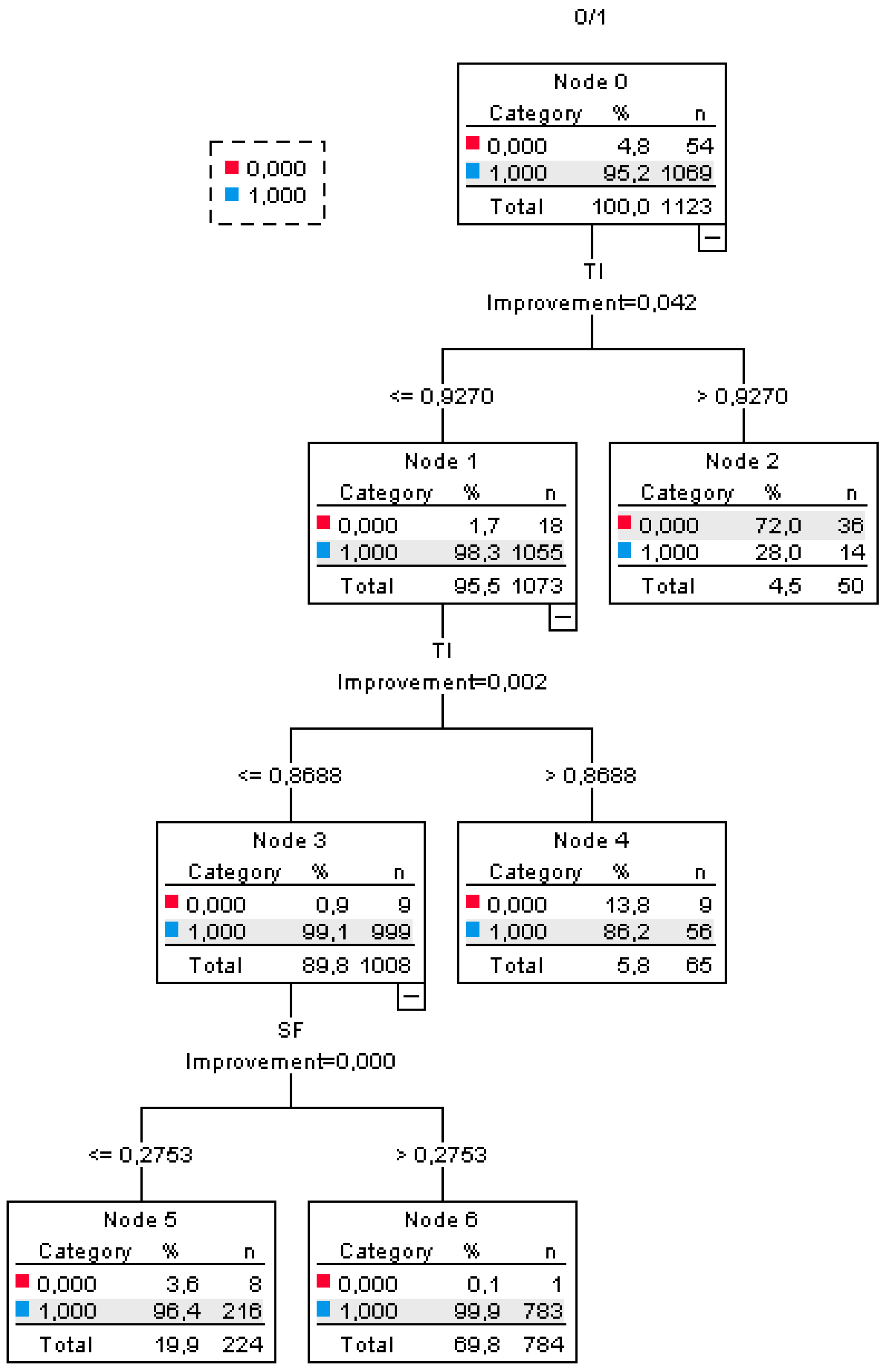
Source: own elaboration.

). In the ANN model, high-importance influential variables include the current indebtedness ratio with an importance of 0.145 (100.0%), followed by the financial independence ratio at 0.131 (90.7%) and the total indebtedness ratio at 0.129 (89.1%). These results illustrate the ANN model’s emphasis on leverage and equity-related metrics. In contrast, the insolvency ratio contributed the least, with an importance of 0.032 (22.1%). The DT model, on the contrary, places most emphasis on the total indebtedness ratio, self-financing ratio, and financial independence ratio, all of which are assigned a rating of 100%. These are the most significant variables for the DT’s categorization. The model further emphasizes leverage, with high priority given to the debt-to-equity ratio and equity leverage at 69% each. However, profitability ratios, including the interest coverage and the non-current indebtedness ratios, were assigned minimal importance in the DT model, with scores of 0% and 3.3%, respectively. To complement the interpretability of the DT, the structure used in this study is visualized in Figure A1.

The performance of the ANN and DT models is evaluated using the key classification metrics of accuracy, precision, recall, F1-score, and area under the curve (AUC). Based on the results in

Table 6. Prediction results and model accuracy.

	AUC	Accuracy	Precision	Recall	F1-Score
ANN	0.9500	0.9637	0.9660	0.9968	0.9812
DT	0.9550	0.9778	0.9869	0.9901	0.9885

Source: own elaboration.

, it is noticed that both of the models have excellent predictive power, with AUC values greater than 0.95, which represents outstanding discrimination ability in distinguishing between financially prosperous and non-prosperous firms. Both models show excellent classification ability, while the DT model does perform marginally better. The AUC reading was 0.9550 with the DT model, while the ANN model scored 0.9500. Regarding accuracy, the DT model is found to properly classify instances 97.78% of the time, in contrast to 96.37% by the ANN. The DT model also performed better in terms of precision at 98.69%, with fewer false positives, while the ANN had a precision of 96.60%. The ANN, however, had better recall, detecting 99.68% of financially troubled companies correctly, while the DT achieved 99.01%. The F1-score that weighs precision against recall was marginally better for the DT at 98.85%, compared to 98.12% for the ANN, as an indication of its overall solid classification accuracy.

Although both models had strong prediction performance, DT outperformed ANN on all the measures of evaluation, except for recall. One of the advantages of DT is that it is interpretable. Unlike ANN, which is a black box and does not provide explicit rules or threshold values, decision trees yield clean decision paths that are easy to understand and enforce by practitioners. This explainability makes DT particularly suitable for financial decision-making contexts, where interpretability is paramount. In contrast, ANN’s lack of interpretability limits its direct practical use, although techniques such as SHAP (SHapley Additive Explanations) or LIME (Local Interpretable Model-Agnostic Explanations) can be employed to develop a better understanding of the impact of single variables on model predictions, thereby making it more practical.

A closer examination of the misclassified samples reveals that both models had difficulties with firms with borderline financial profiles, e.g., intermediate debt levels paired with volatile profitability. The ANN model would sometimes misclassify non-prosperous firms as prosperous, likely due to overfitting against the majority class. Conversely, the DT model would sometimes give false positives, resulting from stringent threshold-based decision splits. These patterns suggest that adding non-financial measures or time-series data, such as management structure or reliance on subsidies, would enhance accuracy in close calls.

5. Discussion

The results presented in the previous section present a general overview of the predictive accuracy and interpretability of the ANN and DT models for agricultural business bankruptcy prediction. In this section, the results are interpreted based on the previous literature, with particular focus on how they support or contradict earlier research findings. Emphasis is placed on the intuitive significance of the relationships found, especially regarding the usability of specific financial metrics and the comparative advantages of the developed models.

Pendharkar [48] and Korol [49] emphasized the debt-to-equity ratio and liquidity indicators as critical parameters in their ANN models used to predict bankruptcy. These two parameters were also emphasized in a study by Behr and Weinblat [50], who utilized random forest models to highlight the importance of such factors in describing complex relationships between financial indicators and bankruptcy risk in different European countries. Mihalovic [51] and Horvathova et al. [52], for Slovak companies, also found the debt-to-equity ratio to be the most important predictor, with ANN models discriminating far more accurately than traditional models. Similarly, Tudor et al. [53] identified that the interest coverage ratio and financial independence ratio are critical predictors in identifying the financial distress of Romanian companies with the assistance of DT techniques. These findings are in line with the importance of the interest coverage ratio and financial independence ratio observed in the findings of the DT model in the present paper, which carried a good level of predictive power for these measures. Interestingly, while both ANN and DT models across the majority of the reviewed research have produced similar trends regarding the relative significance of individual financial variables, the degree to which each variable is accorded significance can vary based on the method used. According to Korol [54] and Vojtekova and Kliestik [112], the ANN models revealed good classification accuracy, with a major focus on factors such as profitability and liquidity. The current indebtedness ratio and non-current indebtedness ratio were shown to be of relatively lesser importance in ANN models, and that is reflective of the same trend in similar earlier work such as that of Radovanovic and Haas [55], where the prominence of liquidity and leverage indicators outweighed other variables. Furthermore, the financial independence ratio is always cited as an important indicator, as in Chen [56], where it was prominently used as a Taiwanese company bankruptcy predictor. His results are consistent with the DT model findings herein, where the financial independence ratio was assigned a high importance value of 100%, confirming its relevance in bankruptcy prediction. The interest burden ratio and debt-to-cash flow ratio, which have manifested moderate significance in the present paper, were also considered in studies like Jeong et al. [57], where the variables related to the ability of a company to generate cash flow and service its debt burden were pivotal. These variables were less impactful in studies such as Mihalovic [51], where profitability and leverage were of more concern than operational measures such as interest burden ratio. Certain variables, such as the insolvency ratio and non-current assets coverage ratio, were less significant in both ANN and DT models in various studies. Korol [54] also pointed out that while insolvency ratios were important, their predictive contribution within models was comparatively lower than that of profitability and liquidity-based variables, which echoes the findings in this study, where the insolvency ratio had very little significance in the ANN model.

Bankruptcy prediction is a globally relevant area of study, with research contributions worldwide that underscore the significance of advanced machine learning methods for improved prediction accuracy. The success of these approaches has been consistently proven across various economies and sectors, and this is an issue of global interest. Several studies point to the excellence of ANN in bankruptcy prediction. Pamuk et al. [58] achieved 82.8% accuracy with an ANN model with 13 variables. Similarly, Shetty et al. [59] achieved 82% accuracy with only five variables, which shows that ANN models can make accurate predictions even when only a few predictors are used. Radovanovic and Haas [55] attained 79% accuracy using an ANN model with 20 variables, while Ben Jabeur and Serret [60] attained 77.34% accuracy using 17 variables. These results confirm that ANNs are capable of detecting intricate patterns in financial data and making good predictions even with heterogeneous sets of variables. Subsequent studies have validated these findings. Kuiziniene and Krilavicius [61] employed an ANN model to detect financial distress, with 92% accuracy, 91% precision, 90% recall, and an F1-score of 90.5%, emphasizing the significance of balance methods such as SMOTE in improving model performance. Similarly, Hamdi et al. [62] attained a high accuracy of 97.80% by applying deep neural networks (DNNs) on Tunisian companies, with a precision of 98.00%, recall of 97.50%, and an F1-measure of 97.75%. Chen et al. [63] also depicted the superiority of hybrid ANN models integrated with genetic algorithms and fuzzy logic, with an AUC of 0.979, accuracy of 96.53%, precision of 96.70%, recall of 96.53%, and an F1-score of 96.58% in Taiwan’s electronics industry. These studies highlight not only the resilience of ANN and deep learning models, but also their applicability in all industries and countries. Comparatively, DT models have worked just as effectively in predicting bankruptcy, often rendering very similar outcomes as ANN models, with the extra benefit of better interpretability. Pamuk et al. [58] registered 82.8% accuracy through a DT model, the same as in their ANN model. Likewise, Shetty et al. [59] experienced 82% accuracy using a DT model, almost the same as their ANN findings. Radovanovic and Haas [55] and Ben Jabeur and Serret [60] had DT models with 79% and 77.34% accuracy, respectively, the same as their ANN performance. Current studies have also continued to affirm the use of DT models. Kuiziniene and Krilavicius [61] were 88% accurate and had an F1-score of 86% for DT models; although lower than the ANN results, they were still helpful because of their clear decision rules. Fasano et al. [64], in a study conducted in Italy, emphasized the interpretability–accuracy trade-off, where a DT model achieved 84% accuracy, 82% precision, and 80% recall, and had an F1-score of 81%. Additionally, ensemble techniques involving DTs have been found to have more predictive accuracy. Njoku et al. [65] employed ensemble learning techniques to improve bankruptcy prediction for financial analysis and obtained an accuracy of 88.5%, precision of 85.2%, recall of 84.1%, and F1-score of 84.6%. Interestingly, most studies indicate that variable counts are not necessarily related to model accuracy. For instance, Garcia [66] used merely six predictors and achieved 73.6% accuracy for DT as well as ANN models. This also demonstrates that the relevance and quality of selected predictors are more important in influencing the efficacy of a model than their numbers. Similarly, Chen [56] demonstrated that SVM was found to be more effective than both DT and traditional models even when fewer financial indicators were used.

Many studies emphasize the superior performance of machine learning algorithms in predicting financial distress and bankruptcy across various sectors. Similar work has also been conducted in Slovakia, confirming the usability of similar techniques for Slovak firms. Among the earlier works, Mihalovic [51] compared traditional statistical methods to machine learning algorithms, namely DT, for Slovak firms’ default risk prediction. The study confirmed that DT models outperformed traditional methods in classification accuracy, with the accuracy rate reaching as much as 83.5%. This confirmed the importance of financial measures such as profitability and leverage in bankruptcy prediction. Horvathova and Mokrisova [68] critically evaluated the limitations of traditional linear regression models and emphasized the need to use more advanced machine learning algorithms, such as DT and ANN, in an attempt to more accurately capture the intricate, non-linear dynamics inherent in financial data. Several more recent research studies have examined the predictive ability of ANN models in the Slovak context. Durica et al. [69] compared ANN and DT models in predicting the financial distress of Slovak firms. The findings were that ANN models performed better overall than DT models, with the ANN model achieving an AUC greater than 0.90 in several cases. Whereas DT models performed poorer in classification, they were valued due to their simplicity and interpretability. In addition, Horvathova et al. [52] utilized both ANN and DT models in the analysis of financial distress in construction companies operating in Slovakia. ANN models achieved better classification accuracy, well over 90%, and DT models were preferred for their ability to create transparent decision rules that make them easier to interpret for stakeholders. Furthering the support with evidence of ANN’s capability for forecasting bankruptcy, Letkovsky et al. [70] further researched its application for company bankruptcy forecasting in Slovakia. Based on the findings, the performance of ANN models surpassed the traditional statistical models, reaching a level of 92%. This goes towards supporting yet further the applicability of ANN models to abstracting intricate financial interdependences and to the characterization of non-linear interdependences among finance variables. Of particular value was the research by Gavurova et al. [71], wherein the non-corporate financial sector in the guise of engineering and automobile industries was the focus sector in Slovakia. Based on figures drawn from 2384 Slovak companies over five years, they constructed an early warning model using a multilayer artificial neural network (ANN) and logistic regression. Their ANN model was found to have high predictive accuracy, with 93.53% accuracy, 92.54% precision, 94.19% recall, and an F1-score of 93.36%. The results confirm the effectiveness of neural networks in modeling complex financial patterns and improving early bankruptcy risk detection in Slovak companies. Similarly, Jencova et al. [72] conducted a study that aimed to predict bankruptcy in Slovak non-financial companies using ANN models. Their multilayer perceptron model, which utilized key financial indicators such as profitability, liquidity, and indebtedness, achieved an accuracy of 86.7%. They also achieved a precision of 85.2%, a recall of 84.9%, and an F1-score of 85%. Although the study did not explicitly mention the AUC value, the results indicate good and well-proportioned performance of the neural network model. The research emphasizes the ability of ANN-based techniques to design effective early warning systems for the Slovak economy.

Besides widely recognized bankruptcy prediction models, there are also some tailored to the Slovak agricultural sector, developed to address its unique fiscal problems, including seasonality, subsidy reliance, and variable investments in assets. Specifically, the model by Chrastinova [113] has helped to discriminate between prosperous and non-prosperous firms, although its simplicity may not be able to capture financial distress dynamics of agro-firms given the background of the volatility of market conditions and external shocks. Similarly, the model developed by Gurcik [114] discriminates enterprises into the same categories. While the two models have been run in the Slovak farming environment, they are constrained in usage by their samples and, by proxy, perhaps generalizability. While useful for preliminary diagnostic use, such conventional models might be supplemented by more advanced methods, e.g., machine learning, that can handle non-linear relationships and provide insights regarding drivers of financial distress to a deeper extent. Valaskova et al. [115] also compared the performance of various bankruptcy prediction models in the Slovak agricultural sector, and the findings concluded that the model by Gurcik [114] was found to exhibit superior predictive accuracy compared to the model by Chrastinova [113]. Valaskova et al. [116] drew on this, conducting a critical examination of bankruptcy prediction models specially formulated for Slovak agriculture. They found that the use of context-specific models pays off, in that those customized for the Slovak agricultural sector yield better results than generic models, particularly in the area of prediction accuracy. Comparatively, AI-based models utilized in this study possess even greater predictive ability. The results achieved with the given models, i.e., AUC of 0.9500 and 0.9550, and F1 measure of 0.9812 and 0.9885, are much better than those of the traditional evaluation methods such as TOPSIS (Technique for Order of Preference by Similarity to Ideal Solution), which are typically applied in agricultural performance appraisal in Slovakia [117]. The AI models, not only with improved predictive accuracy but also with interpretability, are thereby ensured to be a potent tool for enhancing more accurate and actionable bankruptcy prediction in agriculture. These studies demonstrate that while DTs offer good interpretability and clarity, ANNs yield better predictive accuracy and performance metrics in predicting Slovak company bankruptcies. Still, using crucial financial metrics such as profitability, liquidity, and indebtedness is vital for improving model performance for different machine learning techniques.

Generally, these results suggest that policymakers in agricultural finance and rural development may benefit from integrating enhanced predictive models, such as artificial neural networks, into early warning systems for financial distress. The importance of the leverage and liquidity measures, most notably the debt-to-equity ratio and independence from finance ratio, offers an open basis for enhancing financial risk evaluation tools used in subsidy disbursement, credit evaluation, or support programs. Additionally, because of the explainability of decision trees, these types of models may be employed as transparent and readable tools for public agencies seeking to implement rule-based financial management or regulatory decision-making models that are tailored to the specific needs of agricultural enterprises.

6. Conclusions

The extent of indebtedness of agricultural enterprises has a substantial impact on their financial well-being, with excess indebtedness being one of the key determinants of potential financial distress. Since their operations are capital-intensive and heavily dependent on borrowed capital and subsidies, most firms in the sector are prone to heightened financial risks. High debt levels can potentially significantly increase insolvency risk, particularly when it is combined with other determinants such as limited access to financing or market condition instability. Thus, understanding the relationship between indebtedness and insolvency risk is a primary issue in the assessment of the financial condition of agricultural companies. Due to the unique structural and financial characteristics of agricultural firms, such as seasonality, subsidy reliance, and balance sheet asset intensiveness, their classification in bankruptcy prediction models deserves special consideration. This study contrasted the performance of ANN and DT models in forecasting bankruptcy in Slovak agricultural companies. Given the sector’s financial weaknesses, such as expensive operations, price volatility of commodities, and external reliance, the ability to accurately predict financial distress is crucial. The findings confirm that machine learning techniques significantly improve bankruptcy prediction compared to traditional methods, with ANN and DT model displaying adequate classification accuracy.

ANN was superior in prediction accuracy, with an AUC of 0.9500, accuracy of 96.37%, precision of 96.60%, recall of 99.68%, and an F1-score of 98.12%. This all indicates that ANN models are extremely efficient in retrieving complex financial trends, and they are thus an excellent choice when it comes to predicting bankruptcy. Similarly, DT was equally successful, achieving an AUC of 0.9550, accuracy of 97.78%, precision of 98.69%, recall of 99.01%, and an F1-score of 98.85%. The DT model’s slightly better AUC value shows that DT maintains equivalent predictive strength at the cost of interpretability, which is a significant merit in financial decision-making. Analysis showed total indebtedness and self-financing ratios, along with current indebtedness and financial independence ratios, as primary bankruptcy predictors across both models. These findings are in line with previous research, reaffirming the importance of liquidity and leverage ratios in assessing financial well-being. At the same time, the interest coverage ratio and insolvency ratio played a role, indicating that all financial measures do not make an equal contribution to bankruptcy prediction.

Theoretically, this study contributes to the expanding literature at the intersection of machine learning and financial bankruptcy prediction. It reiterates that AI models, even when applied to relatively small and imbalanced datasets, are capable of outperforming traditional linear methods in bankruptcy prediction. The comparison between ANN and DT models also contributes to the understanding of the trade-off between model interpretability and prediction accuracy.

From a practical perspective, this research shows that machine-learning-based models are in strong competition to act as prewarning systems for businesses involved in capital-intensive and high-risk activities such as agriculture. With the capabilities of detecting and quantifying the impact of the best economic measures, such models transfer knowledge into actionable values, which can be infused into ordinary monetary oversight. Their application in bankruptcy forecasting can enhance financial risk assessment significantly, so that policymakers, financial analysts, and business executives can identify financially distressed companies earlier. This early identification can allow them to adopt preemptive restructuring and intervention on a timely basis, thus minimizing the risk of insolvency. This study thus emphasizes the necessity to continue monitoring financial ratios to allow for more predictable forecasting and enhanced financial resilience. For policymakers, the study implies incorporating AI-driven models of bankruptcy predictions in agricultural policy formulation. For managers, the study provides a set of tools that can be embedded in internal management financial systems. Monitoring key financial ratios such as the debt-to-equity, financial independence, and interest coverage ratios makes early warning of financial distress possible and enables strategic intervention at the right time. Such models will be able to strengthen the subsidy program design, enhance credit risk assessment, and inform supervisory regulation, particularly of small and medium-sized agricultural enterprises, which are more vulnerable to adverse financial environments.

This study makes the following contributions to the literature. It experimentally verifies two additional AI models in the previously underexplored setting of Central and Eastern European agriculture, demonstrating their applicability to financial distress prediction. This paper provides a comparative scheme for evaluating ANN and DT strengths and weaknesses for industry-specific prediction. It also paves the way for the extension of machine learning applications to domain-specific, data-poor settings where both interpretability and accuracy are of essential importance.

Despite its contribution, this study has several limitations. The sample is Slovak agricultural companies, and this might restrict the degree to which it can be generalized to other sectors or countries. Although both ANN and DT models were very accurate, their non-parametric and non-linear nature limits the interpretability of the direction of influence (positive or negative) of individual financial indicators. Unlike regression models, which provide signed coefficients, these AI approaches require post hoc tools to infer directional relations. Though ranking importance shows the variables that best predict, it cannot be used tell whether an increase in a particular indicator reduces or enlarges bankruptcy risk. Future research can fill this gap by incorporating explainability frameworks, i.e., SHAP or LIME, to learn more about how differences in input factors influence the calculated value. Additionally, future research might broaden the domain of information with macroeconomic considerations, non-monetary metrics (e.g., governance or weather risk), and exogenous shocks (e.g., pandemics or market dislocation). Although more advanced machine learning techniques like ensemble algorithms (e.g., RF, XGBoost) and deep neural networks (e.g., convolutional or recurrent neural nets) may yield slight improvements in predictive accuracy, this effort specifically emphasized standard and interpretable models. The choice of ANN and DT models was driven by the small sample size and requirements for practicality within the context of agricultural policy, where transparency and ease of interpretation are essential. Yet other advanced techniques, especially when supported by explainable AI architectures, might achieve enhanced prediction capability without sacrificing interpretability. Future research needs to explore these methodologies, particularly as more refined and longitudinal datasets become available.

In conclusion, this study confirms the growing use of artificial intelligence in financial risk analysis. The results confirm that both ANN and DT models provide highly accurate bankruptcy predictions, and they can be applied to assist financial decision-making and ensure economic stability in vulnerable sectors such as agriculture. The results suggest that machine learning techniques need to be integrated more into financial risk management systems, enabling stakeholders with more reliable tools for the prediction and prevention of financial distress.