Article

Comprehensive Assessment of Soil Heavy Metal Contamination in Agricultural and Protected Areas: A Case Study from Iași County, Romania

by
Camelia Elena Luchian
,
Iuliana Motrescu
,
Anamaria Ioana Dumitrașcu
*,
Elena Cristina Scutarașu
,
Irina Gabriela Cara
,
Lucia Cintia Colibaba
,
Valeriu V. Cotea
and
Gerard Jităreanu
“Ion Ionescu de la Brad” Iași University of Life Sciences, 3 M. Sadoveanu Alley, 700490 Iasi, Romania
*
Author to whom correspondence should be addressed.
These authors contributed equally to this work.
Agriculture 2025, 15(10), 1070; https://doi.org/10.3390/agriculture15101070
Submission received: 27 March 2025 / Revised: 30 April 2025 / Accepted: 13 May 2025 / Published: 15 May 2025
(This article belongs to the Section Agricultural Soils)

Abstract

:
Soil contamination with heavy metals poses a significant risk to human health and ecological systems through multiple exposure pathways: direct ingestion of crops, dermal contact with polluted soil, and bioaccumulation within the food chain. This study analyses eleven composite soils, each collected in triplicate from different sites in Iași County, four of which are designated Natura 2000 protected areas (Mârzești Forest, Plopi Lake—Belcești, Moldova Delta, and Valea lui David). The assessment includes measurements of soil humidity by the gravimetric method, pH, and organic matter content, examined in relation to heavy metal concentrations due to their well-established interdependencies. For heavy metal determination, energy-dispersive X-ray spectroscopy (EDS) using an EDAX system (AMETEK Inc., Berwyn, PA, USA) and X-ray fluorescence spectrometry (XRFS) with a Vanta 4 analyser (Olympus, Waltham, MA, USA) were employed. Additionally, scanning electron microscopy (SEM) with a Quanta 450 microscope (FEI, Thermo Scientific, Hillsboro, OR, USA) was used primarily for informational purposes and to provide a broader perspective. In the case of chromium, 45.45% of the samples exceeded the permissible levels, with concentrations ranging from 106 mg/kg to 186 mg/kg, the highest value being nearly twice the alert threshold. Notably, not all protected areas maintain contaminant levels within safe limits. The sample from the Mârzești Forest protected site revealed considerably raised concentrations of mercury, arsenic, and lead, exceeding the alert thresholds (1 mg/kg—mercury, 15 mg/kg—arsenic, and 50 mg/kg—lead) established through Order no. 756/1997 issued by the Minister of Water, Forests, and Environmental Protection from Romania. On the other hand, the sample from Podu Iloaiei, an area with intensive agricultural activity, shows contamination with mercury and cadmium, highlighting significant anthropogenic pollution. The findings of this study are expected to raise public awareness regarding soil pollution levels, particularly in densely populated regions and protected ecological zones. Moreover, the results provide a scientific basis for policymakers and relevant authorities to implement targeted measures to manage soil contamination and ensure long-term environmental sustainability.

1. Introduction

Soil represents an essential ecosystem that provides valuable services for the supply of food, energy, and raw materials. It facilitates carbon sequestration in chemical compounds, supports water purification and infiltration, and regulates nutrient cycles through the activity of microorganisms [1]. It is estimated that 95% of food is produced directly or indirectly using soil as a support for plants and animals [2]. Heavy metals are naturally found in soil due to pedogenetic processes of parent materials, chemical processes within the earth, or from biological residues, having levels that are considered trace and are rarely toxic [3,4,5]. Due to different soil types and parent materials in different regions, the natural concentrations of heavy metals in soil vary widely. Usually, natural pollution with heavy metals constitutes the primary source of soil heavy metals, especially in areas with less human disturbance [6] such as protected areas. This is not the case when those preserved areas are situated near high traffic zones (in the case of Valea lui David, which is close to the E85 road, or of Mârzești Forest, which is near the DJ282 road) or are close to areas with intensive agriculture leading to pollution through atmospheric deposition [7]. In this instance, natural sources are not the main contributors to soil pollution with heavy metals [8,9,10].
The mobility and bioavailability of heavy metals in soil depend on many factors such as pH, organic matter, cation exchange capacity, soil texture and humidity, and the presence of competing ions [4]. Large-scale contamination has occurred, especially with the development of anthropogenic activities. The primary anthropogenic sources generating heavy metals are as follows: industrial processes; mining; foundries and smelters; coal burning in power plants; fossil fuel and oil burning; waste incineration; improper storage of electronic waste (used metals in batteries, semiconductors, and circuits); lamination; dyes and paints; the plastic, chemical, and wood industries; nuclear power plants; municipal waste, sewage, and the use of pesticides and fertilisers in agriculture; land irrigation with the help of waste water; automobile emissions; atmospheric deposition; etc. [11,12]. The primary sources of heavy metals are detailed in Table 1.
Heavy metals can be transported long distances from their original sources, with one study showing how heavy metals create different patterns of toxicity [13]. The excess of metal pollutants deposited on the soil can be transformed and stored in plants, which leads to a decrease in crop productivity, from where, through the food chain, they reach animals and humans [14,15,16]. Excessive levels of heavy metals can harm organisms, vegetation, and ecosystems by disrupting vital metabolic functions, primarily affecting biological characteristics such as the total microorganism presence in soil, species diversity, and microbiological and enzymatic activity. In addition, heavy metals alter the humus content, structure, and pH of soils [17]. These processes lead to a partial or, in some cases, complete loss of soil fertility. Any increase in pollutant emissions can adversely affect crop productivity [18]. Soil pollution can harm human health because toxic substances can bioaccumulate in crops and can seep into groundwater. Due to its properties and structure, the soil acts as a filter that can retain and store toxic elements. Exposure to heavy metals is usually chronic (exposure over an extended period) due to transfer through the food chain. Acute (immediate) heavy metal poisoning is rare but possible through ingestion or skin contact [19]. The individual health effects of heavy metals are described in Table 1.
At the same time, Cu, Mn, Fe, and Zn have a dual role as trace elements. They are essential in the biological metabolism of plants, the immune system of animals, and human health [20]. Deficiencies of any of these trace elements can lead to undesirable pathological conditions. Soil contamination with heavy metals caused by anthropogenic activities has become an environmental concern because of the potential adverse effects on many organisms. Heavy metals can occur naturally in low quantities in soil and in high concentrations, they present acute and chronic toxicity due to their persistence over time. Heavy metals leach from the aforementioned sources into soil and plants. At the food chain level, bioaccumulation and biomagnification manifest themselves within animal organisms and implicitly within human organisms through the appearance of chronic pathologies [21].
Table 1. Sources of heavy metal soil pollution and their effects on human health.
Heavy MetalSourcesEffects on Human HealthReferences
Aluminium (Al)Steel industry
cutlery; pots and pans
Nausea; vomiting; mouth and skin ulcers; skin rashes; arthritic pain; diarrhoeal disease; possible onset factor of Alzheimer’s disease; memory loss; vertigo and dizziness; bone and brain damage[19]
Arsenic (As)Pesticides; herbicides; insecticides; rodenticides; treated wood products; colouring agents for textiles; mining; wallpaper; toy industry; ash resulting from coal combustionVisceral neoplastic pathologies: liver, kidney, lung, bladder; epithelial neoplastic pathologies; circulatory disorders[22,23,24,25]
Barium (Ba)Equipment for industrial controlCardiac arrhythmias; respiratory failure; gastrointestinal dysfunction; muscle spasms; high blood pressure[23]
Beryllium (Be)Coal; rocket fuelsCarcinogenic compound in acute/accidental/chronic exposure[23]
Cadmium (Cd)Fertilisers; metallurgical industry; spoiled food; cigarettes; manufacture of plastic materialsKidney damage; prostate dysfunction; bone pathologies; neoplasia; lung damage; disturbance of calcium metabolism[23,26,27]
Chromium (Cr)Leather tanning; metal refining; textile dyeing; pharmaceutical industry; ink and pigments; refractory materials; wood preservatives; fungicidesNeoplasms; nephritis; ulcerations; hair loss; diabetes; feeling of nausea; headaches; genetic/congenital diseases[23,28,29,30]
Cobalt (Co)Mining industry; wood conservation; metal industry; graphic industry; electronics; medical assistanceDiarrheal disease; arterial hypotension; paresis; damage to striated, smooth, and cardiac muscle tissue; muscle weakness; obtundation[23,31,32]
Coper (Cu)Pesticides; insecticides; treated wood productsTissue destruction in the brain and kidneys; elevated levels are commonly associated with cirrhosis of the liver[23,33]
Iron (Fe)Building materials (asbestos); mining industry (iron smelting and steel smelting); car constructionIron toxicity depends on the dose/chemical form and the exposure period: 6 h after the overdose, gastrointestinal/local effects appear (gastrointestinal bleeding, vomiting, and diarrhoeal disease); 6–24 h after the overdose, the latency period sets in (apparent improvement of local symptoms); at 12–96 h systemic and hepatic toxicity sets in (shocks, lethargy, tachycardia, arterial hypotension, hepatic necrosis, metabolic acidosis, and death); within 2–6 weeks of administration late gastrointestinal effects appear (ulcerations and strictures/obstructions); asbestosis (second leading cause of lung cancer);
cell death
[19,34]
Manganese (Mn)Foundries; smelters; steel industry; ceramics; fireworks; dry cell batteries; fertilisers; fungicides; paints; medical imaging agent; cosmetics; additive in gasoline to improve the octane number; food (cereals, beans, nuts, and tea); mining activities; car exhaust; cigarette smokeNeurological disorders, the combination of neuropsychiatric symptoms = ‘manganism’; inhalation causes lung damage (pneumonia); crosses the blood–brain barrier and the placental barrier; infertility; nephropathies and renal lithiasis; carcinogenic potential; associated with Parkinson’s disease, schizophrenia, and hypertension[35]
Mercury (Hg)Thermometers and barometers; tensiometers; amalgam for dental restoration; fluorescent lighting; in the production of caustic soda; in the preservation of pharmaceutical products; nuclear reactors; antifungal agents for the woodworking industryGastrointestinal toxicity; neurotoxicity; nephrotoxicity; depression; sleepiness; asthenia; hair loss; insomnia; memory loss; restlessness; visual disturbances; tremors; tantrums; brain injuries; renal and respiratory failure[23,36]
Nickel (Ni)Plating industry; fossil fuel burning; mining; cigarette smoke; jewellery; shampoos; detergents; coinsCarcinogenic embryotoxicity; teratogenesis[23,37]
Lead (Pb)Plastic materials; (automatic) vehicles; hair dyes; paints; paint varnish; pipes; batteries; gasoline; enamelled productsDecreased intelligence quotient (mental retardation); memory loss; infertility; alternating mood; sterility; risk of cardiovascular disease[23,38,39]
Tin (Sn)Preservatives and dyes for wood; biocides; food industry; brazing alloys; dental amalgams; aircraft engineering (titanium alloys); foil; reducing agents in the manufacture of polymers, toothpaste, ceramics, porcelain, enamel, drill glass, and inks; pigments in the ceramic and textile industry (purple tin); manufacture of tin salts for chemical plating reagents; perfume stabiliser; as SnO2 for glass makingHigh concentrations: haemolysis; ecotoxicity; skin rashes; stomach ache; vomiting; diarrhoea; abdominal pain; headaches; palpitations; possible cytotoxicity
Low concentrations: fatigue; depression; low adrenals; breathing difficulties; asthma; headache; insomnia
[40]
Zinc (Zn)Fertilisers; paints; rubber; cosmetics; plastic products; pharmaceuticals; inks; soaps; textiles; batteries; electrical equipmentDizziness; fatigue; vomiting; kidney damage; cramps[23,38,41]
Combating this type of contamination requires an integrated approach using modern monitoring technologies, comprehensive legislation and, perhaps most importantly, public education. Adopting strategies to minimise and restore affected ecosystems requires collective engagement to protect the environment and human health.
This article investigates the current state of heavy metal contamination of soils originating from Iași County (Romania). Eleven samples were analysed regarding the metal content assessment and the soil‘s physicochemical properties. This study‘s originality comes from its ground-breaking examination of heavy metal pollution in soils from protected and agricultural regions, an understudied topic for which there is currently no available published data. By employing fast, cost-effective analytical techniques such as X-Ray fluorescence spectrometry (XRFS) and energy-dispersive spectroscopy (EDS), this study provides a practical approach to assessing contamination levels in areas influenced by diverse anthropogenic pressures, including agriculture, industry, and research. This integrated approach not only fills a critical data gap but also offers a replicable model for rapid contamination screening in similar regions across Europe.

2. Materials and Methods

2.1. Climate and Environmental Conditions of the Study Area

Iași County is located in the north-eastern part of Romania, limited to the west by the Moldova River and to the east by the Prut River, which also forms the border with the Republic of Moldova. Covering an area of 5476 km2, it has approximately 1,008,254 inhabitants, with an average population density of 174 people per km2. Iași is a medium-sized county, accounting for 2.3% of the country’s total area and ranking 23rd among Romania’s counties (Figure 1).
The thermal regime records multiannual average temperatures ranging from 8 °C in the hilly regions to 9.6 °C in the plains. Precipitation levels are relatively low across the entire county, averaging 500 mm annually in most areas and reaching up to 600 mm per year in the western part [43]. From a geological perspective, the area of Iași County partially overlaps with all the geographical units of the Moldavian Plateau: the Suceava Plateau to the west, the Bârlad Plateau to the south, and the Jijia Hilly Plain in the centre, north, and east. The region has a pronounced sculptural character, consisting of plateaus and long hills that gently slope toward the southeast.

2.2. Soil Sample Collection

Samples were collected in triplicate from the topsoil layer, ranging from 0 to 30 cm in depth, from 3 different points, with specific weights varying between 1.5 and 2.0 kg, in accordance with the requirements for physicochemical analysis. The triplicate samples collected from each of the eleven locations were combined to form a single composite sample per location. Stainless steel equipment was used during the collection process to prevent contamination. The soil samples were then securely sealed in plastic bags and labelled with unique identification numbers [44]. The sampling was carried out from 11 distinct areas (Figure 1).
The soils sampled from the mentioned regions are mainly of the chernozem or chernozem combined with phaeozem types. The soil classification and the dominant economic activity for each area can be seen in Table 2.

2.3. Physicochemical Parameters

Physicochemical analyses were performed in triplicate for each sample and focused on soil moisture, organic carbon, humus content, and pH. Quality control check samples and reference materials were used according to the published literature [47]. All reagents were analytical grade and supplied by Merck KgaA (Darmstadt, Germany).

2.3.1. Determination of Soil Humidity

The soil samples were air dried, mechanically ground (Retsch RM 200 equipment, Haan, Germany), sieved through a 2 mm sieve to obtain the fraction used for each soil analysis, and stored at 4 °C. Humidity was determined by weighing approximately 5 g of soil and using the gravimetric method, in an oven at 105 °C. The sample was left to cool in a desiccator and then brought to constant mass by successive weighing on an analytical balance. This parameter is expressed as a percentage [48,49].

2.3.2. Determination of Organic Carbon and Estimation of Soil Humus Content

The most critical parameter of the humus content in the soil is organic carbon, which constitutes 43–62% of the soil’s chemical structure, and differs depending on the time of formation, the soil’s nature, and other conditions. The Walkley–Black method, modified according to the literature [48,50,51], was used to determine the organic carbon through oxidation in the presence of dichromic anhydride and sulfuric acid, maintaining the sample at a constant temperature of 100 °C for 20 min. One gram of crushed, dry soil was used along with the aforementioned chemical reagents. This mixture was placed in the oven at 92–97 °C for 30 min. After cooling, 3–5 drops of diphenylamine indicator were added to facilitate titration with Mohr’s salt until the colour changed from blue-violet to dirty green.

2.3.3. pH Evaluation

The working method used to determine pH involved weighing approximately 10 g of soil from each sample, which was then brought into solution. The values were determined using the WTW Multi 3320 (Weilheim, Germany) device at a temperature of 21.5 °C. Between readings, the electrode was rinsed with distilled water [48,52]. The evaluation of the soil pH is presented in Table 3.

2.4. Heavy Metal Analysis

Two methods were used for heavy metal analysis: EDS and XRFS. Since EDS is less accurate, it is used in conjunction with SEM, which is primarily for informational purposes and to provide a broader perspective. XRFS, on the other hand, is faster and offers higher precision.

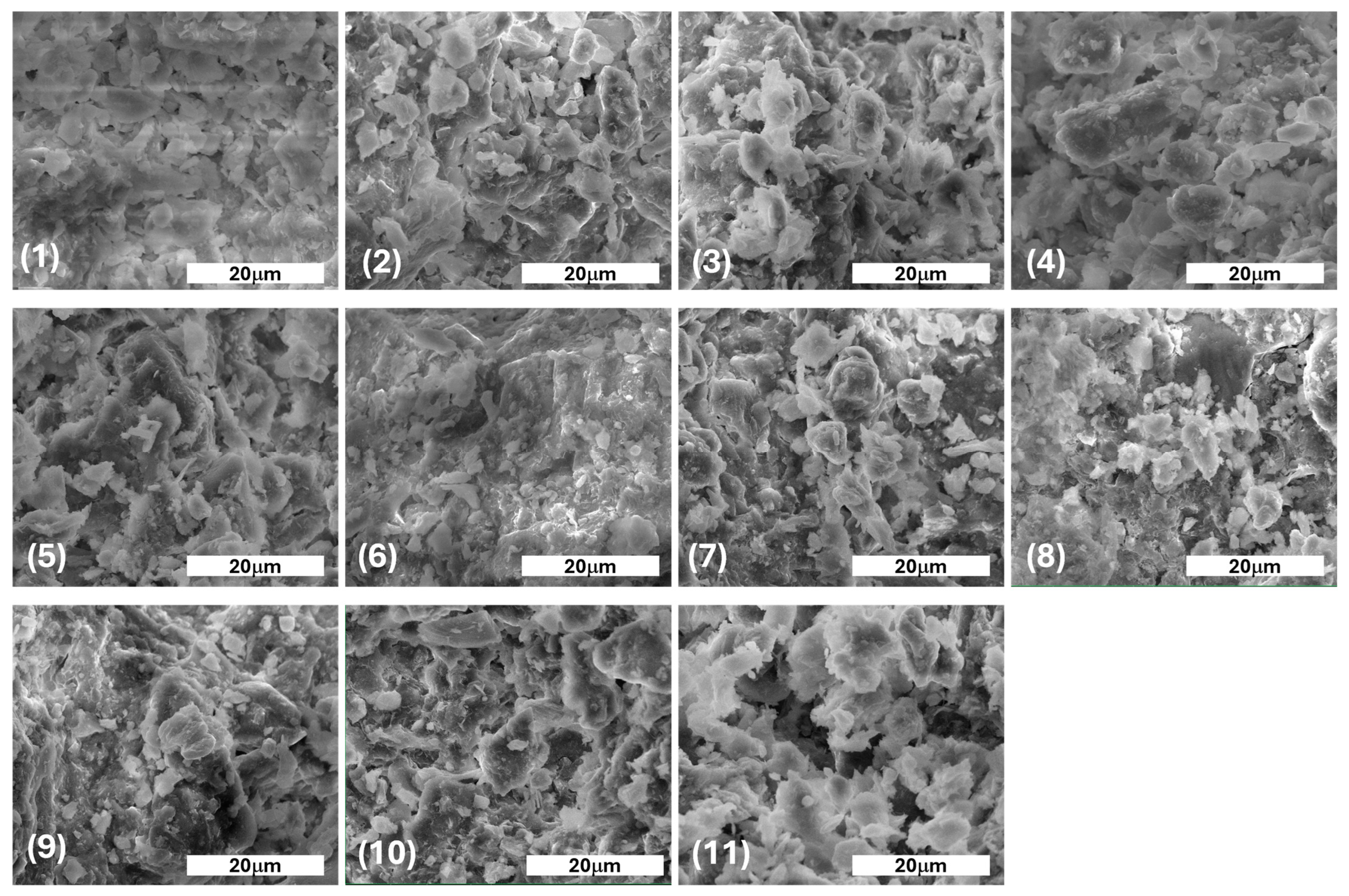
2.4.1. Micro-Imaging of Soil Samples Using Scanning Electron Microscopy

The scanning electron microscope (SEM) is an advanced piece of equipment used to analyse the surface of materials. In the SEM technique, the sample is bombarded with a focused electron beam having an acceleration voltage of 30 kV [53]. As the electron beam collides with the sample, several signals are emitted, which are further picked up by detectors. These detected signals are processed to produce an image [53].
When exposed to the electron beam, ‘elastic scattering’ occurs via interactions with the outer shell electrons or the atomic nucleus at similar energy levels. Electrons elastically scattered at angles greater than 90 degrees are called backscattered electrons (BSEs). The information received based on BSE is beneficial for understanding the compositional and topographical features of the specimen. On the other hand, when incident electrons collide with the sample atoms and electrons, ‘inelastic scattering’ occurs. In these inelastic interactions, the accelerated electrons transfer substantial energy to the specimen atoms, where the sample electrons are excited and secondary electrons (SEs) are generated, which typically possess energies below 50 eV [54]. SEs are used mainly as a signal in SEM because the electrons emitted are low in energy; as a result, they can originate only from a region that is a few nanometres distant from the sample and hence give accurate topographical information with excellent resolution [54].
The soil samples were micro-imaged using a Quanta 450 (FEI, Thermo Scientific, Hillsboro, USA) in this work. The microscope is an environmental SEM and does not need any prior preparation of the samples, so they can be imaged as they are. The soil was fixed using double-sided carbon tape onto aluminium stubs, then analysed using a 15 kV accelerated electron beam at low pressure (approx. 10−4 Pa).

2.4.2. Initial Evaluation of Elemental Composition Using Energy-Dispersive X-Ray Spectroscopy

Energy-dispersive X-ray spectroscopy (EDS) constitutes a sophisticated analytical technique employed to quantify variations in the elemental composition of nanomaterials within a defined sample. This methodology is implemented in conjunction with scanning electron microscopy (SEM) [55]. This technique employs X-ray excitation to ascertain the presence of specific chemical elements within a sample (qualitative analysis) or to evaluate their relative concentrations (quantitative analysis). In the realm of quantitative analysis, the concentration of an individual element within a sample is quantified through the measurement of peak intensities. Given that each element possesses a distinctive atomic configuration that produces a unique array of peaks on its electromagnetic emission spectrum, qualitative analysis involves the identification of various X-ray peaks located at predetermined positions within the spectrum [56].
This is not an accurate technique for surface determination because X-rays get information from a depth depending on the chemical composition of the analysed sample. During energy-dispersive X-ray spectroscopy (EDS) analysis, the electron beam is systematically directed across the specimen to generate an image representing the elemental distribution within the samples. This analytical procedure typically requires an extended duration, often spanning over several hours. In the context of EDS, the composition and concentration of heavy metal ions present in the nanoparticles, particularly those situated at or near the surface of a specimen, can be quantitatively assessed; however, elements possessing atomic numbers lower than 11 present significant challenges for detection via EDS methodologies [57]. In this case, the soil samples were analysed as they were after the soil sample’s imaging by SEM, quantifying the elemental composition using an EDS detector (EDAX, AMETEK Inc. Berwyn, PA, USA). For each sample, three areas were measured, and the operating software evaluated the relative concentrations of the elements after the background setting. The data are presented as averages with standard deviations determined from the three measurements. The EDS analysis was conducted using the TEAM version V4.1 system with prior calibration using a standard AlCu sample.

2.4.3. Determination of Heavy Metal Content by X-Ray Fluorescence Spectrometry

X-ray fluorescence spectrometry (XRFS) was carried out using a portable device (Vanta 4, Olympus, Waltham, MA, USA) that allows fast and efficient detection of heavy metals in soil through in situ or ex situ measurements. Because the XRFS method is entirely non-invasive, samples collected and measured in the field can be analysed in the laboratory without modification [58]. The principle of XRFS states that when an X-ray emission from a radioactive source encounters a sample, the X-rays can either be absorbed by atoms or scattered through the material. After absorption, the atoms become ‘excited’ and emit some X-ray characteristic photons to an energy level unique to each element [58]. Identifying the energy level of the emitted X-rays is used to identify the present metal species and measure the energy of the emitted X-ray, which gives a quantitative indication of the metal concentration in the sample. The results are expressed in parts per million (ppm) with confidence values provided by the device [58].

2.5. Pollution Assessment Methods of Heavy Metals

2.5.1. Contamination Factor and Degree of Contamination as Indicators of Soil Pollution—Method Description

The contamination factor (CF) is used for defining the contamination factor for each metal, and it is calculated with the following formula:
CF = C   metal C   background   value
where C metal refers to the metal concentration and C background value refers to the value of reference assigned to each element [59].
The subsequent terminologies are utilised to elucidate the contamination factor: CF < 1 signifies a low contamination factor; 1 ≤ CF < 3 denotes a moderate contamination factor; 3 ≤ CF < 6 indicates a significant contamination factor, and CF ≥ 6 represents a very high contamination factor [59].
The degree of contamination (DC) equals the sum of all CFs, visible in Formula (2). The subsequent nomenclature was employed to characterise the degree of contamination (DC values) for the specified metals: DC < 6: low degree of contamination; 6 ≤ DC < 12: moderate degree of contamination; 12 ≤ DC < 24: considerable degree of contamination; and DC = 24: very high degree of contamination signifying severe anthropogenic pollution [59].
DC = CF1 + CF2 + CF3 + … + CFn

2.5.2. Assessment of Soil Contamination Using the Pollution Load Index

All of the locations were assessed for the level of metal contamination based on the formula formulated by [60]:
PLI = CF 1   ×   CF 2   ×   CF 3   × ×   CFn n
where n is the number of metals examined, and CF is calculated for each metal according to Formula (1).
The pollution load index can be measured on a scale from 1 to 6, where 0—no pollution, 1—none to medium pollution, 2—medium pollution, 3—medium to strong pollution, 4—strong pollution, 5—strong to extreme pollution, and 6—very strong pollution [60].

2.5.3. Geo-Accumulation Index as a Tool for Assessing Soil Pollution

The geo-accumulation index (Igeo) is calculated to assess the extent of anthropogenic pollution and to evaluate various metal concentrations within the soil [61]. Igeo is calculated with the following formula:
I geo = log 2 Cn     1.5   ×   Bn
where Cn is the measured concentration of the heavy metal found in the soil sample in mg/kg, Bn refers to the background value assigned to each element, and the 1.5 factor is used to reduce the potential fluctuations in the background value that may be attributed to lithogenic influences [61].
Förstner et al. [62] enumerated the geo-accumulation categories along with the associated levels of contamination: Igeo ≤ 0: practically free from contamination; 0 ≤ Igeo ≤ 1: free from contamination to moderately polluted; 1 ≤ Igeo ≤ 2: moderately polluted; 2 ≤ Igeo ≤ 3: moderately to severely polluted; 3 ≤ Igeo ≤ 4: severely polluted; 4 ≤ Igeo ≤ 5: severely to extremely polluted; and 5 < Igeo: extremely polluted.

2.6. Statistical Analysis

To highlight the relationships between the physicochemical parameters of the analysed soil samples, the metal content, and the pollution assessment indexes, the XLSTAT BASIC ACADEMIC 2024 software (Lumivero, Denver, CO, USA) was used. PCA (Principal Component Analysis) and correlation tests were performed in this regard.

3. Results and Discussions

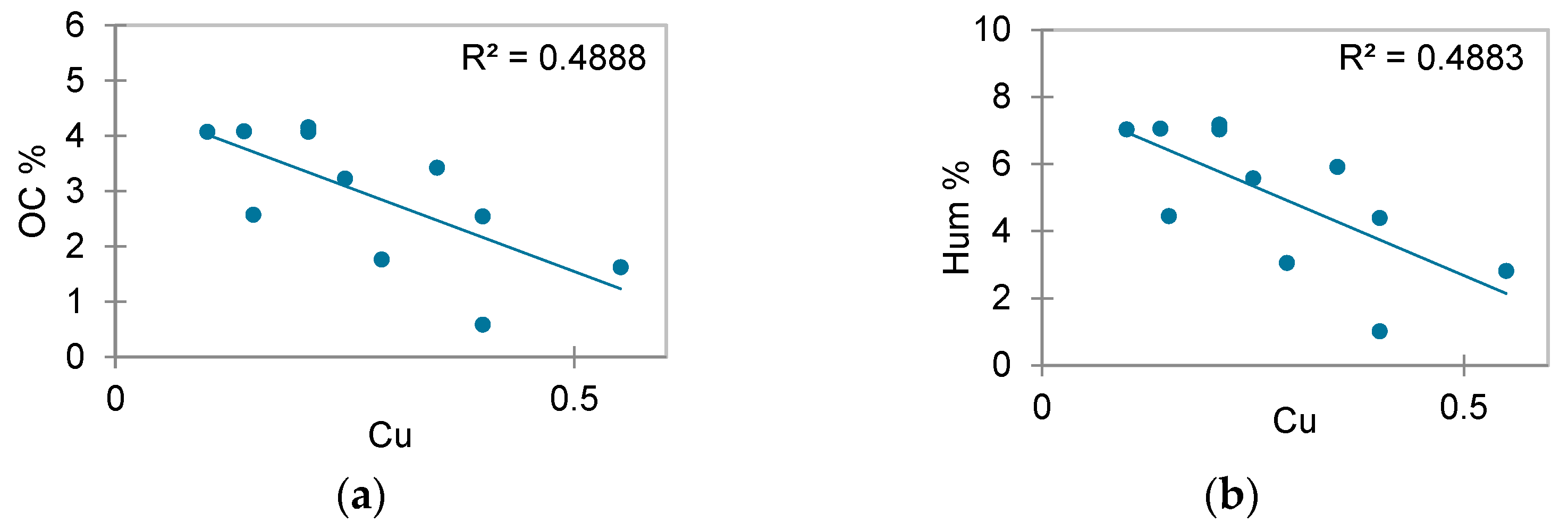
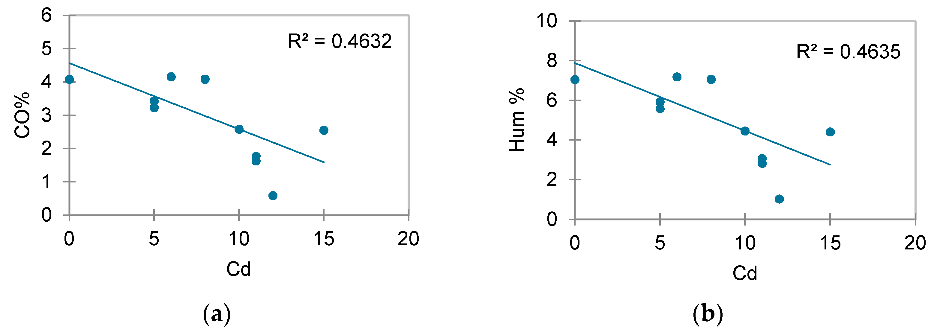
3.1. Physicochemical Properties

Table 4 highlights the humidity, organic carbon content, humus content, and soil pH determination results. The soil humidity varied for all samples between 11.58% (S6) and 23.3% (S8). Samples S1, S2, S3, S5, S9, S10, and S11 are close in value. Samples S4 and S7 were the average samples closest in value.
The humus content is calculated using the organic carbon content, varying from 1.02 (S6) to 7.18 (S8). Most samples show a slightly alkaline reaction.
pH plays a significant role in determining the bioavailability or immobilisation of heavy metals [63]. Consequently, there exists a direct relationship between the soil’s capacity to retain heavy metals and pH (achieving its peak near neutral pH), coupled with an inverse correlation between pH and the accessibility of elements such as Cu, Mn, and Zn (the availability of these elements for plant uptake diminishes as pH increases within the range of 5 to 8). The pH values ranged from 5.146 (slightly acidic) to 8.492 (moderately alkaline). S8 had a moderately alkaline pH, while S1, S3, S4, S5, S6, S7, S10, and S11 had a slightly alkaline pH. S2 was the only solution with a pH below 6.81 and a slightly acidic reaction, corresponding to forest soil. The neutral sample was sample S9, with a pH of 6.833. This can be because it is a commercial orchard where various amendments or specific treatments are applied, because most food crops flourish within a soil pH range of 5.5 to 7.0. Similarly, Liu and Hanlon [64] postulated that when the soil pH drops below 5.5, Al, Fe, and Mn solubility increases significantly. Elevated levels of Al and Fe can bind with phosphate, reducing the availability of phosphorus to plants. At the same time, Ca and Mg levels may be insufficient to meet crop needs. Conversely, when the pH exceeds 7.5, Ca and Mg may be in excess, while Fe and Mn may become less available for plant uptake. Additionally, excess Ca and Mg ions can cause phosphate to precipitate, potentially leading to phosphorus deficiencies in crops grown in high-pH soils.
By the classifications defined by international organisations [65], the soil samples from the investigational area can predominantly be categorised as slightly alkaline soils (72.73%). This category was followed by slightly acidic, moderately alkaline, and neutral, each with 9.09%.
Most of the pH samples align with the moderately alkaline soil classification (7.324–8.492). Given the neutral sub-alkaline conditions, the significance of this parameter regarding the distribution of heavy metals is notably limited, thereby substantially constraining their mobility [66].

3.2. Heavy Metal Quantification

Besides visualising the microstructure of the soil samples, the electron microscope (EDS) was used to determine the relative elemental composition. The values are presented in Table 5 as averages for three analysed areas in each case, with the average standard deviation.
Table 6 presents the XRFS results, which are expressed in parts per million (ppm) (1 ppm = 1 mg/kg), according to Tóth et al. [67]. Data on the CF, DC, and PLI for the metals analysed with XRFS are highlighted in Table 7.

3.2.1. Soil Characteristics Using SEM

Figure 2 shows the microstructure images of areas corresponding to the analysed soil samples at the same magnification. At first glance, the appearances seem very similar. However, several differences can be noticed in the distribution and size of soil aggregates. In some samples (such as S1, S4, S5, and S6), the soil aggregates look compacted together, and are much loosened in other samples (S2, S3, S5, S7, and S11). On the one hand, this can be linked with soil humidity (Table 4), with low-humidity soils being more compacted than those with higher moisture and humus content. In this regard, S6 looks the most compacted (Figure 2(6)) and looks like it the one with the lowest humus content. The grain size is directly linked with the soil’s permeability for water, air, and nutrients, determining the porosity. These factors might strongly influence the movement of heavy metal contaminants in the deeper soil layers and thus should always be considered. It was also shown that heavy metals can reduce porosity and produce clogging.

3.2.2. EDS Results

The EDS measurements in Table 5 show that, in this case, analysing a small area of the soil samples does not provide reliable results regarding heavy metal contamination. Not only is it a semi-quantitative method, but it is also hard to compare results between the samples since it offers a relative amount of an element. It also analyses a small area that could not be representative of the analysed sample.
Soil pH and organic carbon were found to be associated with the vertical movement of heavy metals such as Pb, Zn, Cd, Cu, and Mn. The highest values of the coefficient of determination were obtained for the relationship between Cu and the proportion of organic carbon and humus (R2 = 0.48). Nevertheless, it is a low dependence of the mentioned parameters, as other factors may influence the accumulation of Cu in the soil (Figure 3). According to the results, in acidic soils (low pH), heavy metals such as Cu become more mobile and available [68], while in alkaline soils (high pH), they tend to precipitate and be less available [69]. Therefore, it is essential to focus on soil properties rather than the contamination, such as trying to establish connections and understanding their migration in deep soil layers as a first step in taking remediation measures [70]. Thus, one conclusion is that XRFS is a faster and more accurate method compared to EDS.

3.2.3. XRFS Results

According to XRFS, for Mn, Cu, Ni, and Zn there is no excess in any of the samples. For Cr, for 45.45% of the samples an excess was found, namely S4, S5, S9, S10, and S11, which range from 106 mg/kg for S10 to 186 mg/kg for S11, the latter being almost double the alert threshold value. Nine of eleven samples have values over the alert threshold limit for the less sensitive soil type for Co (Table 6), except S1 and S2. The highest values, two times over the alert threshold, are observed in the case of S4 and S10. Regarding arsenic, S1, S4, S5, and S9 are below the limit value. A total of 63.63% of the samples have high values. For six samples, S3, S6, S7, S8, S10, and S11, there is an excess of two to six units, which can be considered negligible. For sample S2, the measured value is 959 mg/kg, which is 38.36 times higher than the allowed limit. Cadmium was found under the alert threshold in the case of the less sensitive soil, with the other samples having values four to ten times higher than the limit. Apart from S2, higher values than the limit were recorded for the other ten samples in the case of cadmium.
According to Figure 4, the organic carbon content appears to have a moderate impact on the distribution of Cd in soil. The other metals have a weaker correlation with organic carbon, suggesting that additional factors influence their distribution.
Regarding Hg, two samples had values over the detection limit: one was higher than the alert threshold value by one unit, while the other sample was 19.5 times higher. As such, there is a correlation between an increased amount of Hg in acid forest soils [71]. Al is one of the most abundant metals in the atmosphere, and is largely insoluble and therefore harmless. Increased acidity is the leading cause of Al mobilisation [72]. According to Table 4, the sole sample with acidic pH was S2, which had the lowest Al content (as seen in Table 4).
The soils from which the sampling was carried out are predominantly of the chernozem type (Table 2). According to Jonczak et al. [73], chernozems are moderately abundant in total Fe and Al. Soil structure is the result of elementary soil particles being bound together at specific points on their surface by cementing substances such as organic compounds, iron and Al oxides, colloidal silicon, or calcium carbonate (CaCO3) [74]. The relative importance of these stabilising agents depends on their nature and abundance in the soil. Therefore, elevated Al and Fe concentrations indicate a normal soil structure. Low values of Al and Fe can be observed in S1 and S2.
Sample S2 exhibited the highest level of As and Pb (40.7 times higher than the allowed limit), raising the question of whether the latter two are connected. As the area is now a protected natural site and it has been a forest for many years, one explanation could be due to the battles that took place there during World War I, as some reports indicate heavy metal contamination as a result of the artillery used during that period [75,76]. The same sample shows the lowest values for Al and Fe. This is the only sample with acid pH, which could be an aggravating factor along with the abovementioned situation.
The pH value and organic matter appear to be important factors controlling the geochemical behaviour of heavy metals like Pb and Hg [77], and soil acidification results in an increase in the effective fraction of Pb and Hg [77]. Exceeding values of Hg, Cd, and Co in the case of variant S10 can be explained by the chemical treatments applied to the crops [78]. Figure 5 illustrates a strong relation between the accumulation of Hg, As, and Pb levels in soils and pH value (R2 > 0.75), while a low correlation was observed for Ni, Zn, Fe, Co, Mn, and Zn concentrations. This highlights the influence of pH on metal solubility and mobility. Thus, the concentrations of metals accumulated in the soil are inversely proportional to the pH value for Hg, As, and Pb, and inversely proportional for the other metals represented in Figure 6.
For European soils, mean background value contents have shown a decrease over the years, highest in 2005 [79], almost halved, according to Mico et al. [80], in 2007, and just slightly lower in 2016 [67], except for Pb, where Tóth et al. [67] found the lowest value of them all. For the metals in this study, Co and Cu show exceedances for European soil. The Netherlands’ baseline values [81] are between the values for European soil, except for As, Cu, Pb, Sn, and Zn, where the values surpass those observed within European contexts. This study’s values are below those in the Netherlands for As and Pb, except S2, and for Zn, except S4. The world soil average has an increase in baseline values from 1992 [82] until 2010 [3], except for Cd and Hg. The range of values for chernozems on the world scale predominantly spans within the values for world soils, [3,82], except Cd and As, which exhibit higher values exceeding both extremes, or Pb, which presents the only lower value. In accordance with the legislation in force, normal values in Romania fall between those in Europe and those worldwide [83]. The only one above Europe and the world is the normal value of Mn.
Table 6. Heavy metal concentrations (mg/kg) in soil determined using XRFS.
SamplesAlCrMnFeCoNiCuZnAsCdHgPbSn
S12893 ± 534<LOD *40 ± 5150 ± 518 ± 2<LOD *53 ± 227 ± 16 ± 15 ± 1<LOD *2 ± 1<LOD *
S21312 ± 32323 ± 740 ± 4<LOD *16 ± 2<LOD *36 ± 112 ± 1959 ± 9<LOD *78 ± 210,176 ± 32<LOD *
S37546 ± 81685 ± 13866 ± 1626,884 ± 112174 ± 1647 ± 346 ± 3117 ± 321 ± 111 ± 1<LOD *14 ± 168 ± 7
S48580 ± 809119 ± 13816 ± 1530,571 ± 118209 ± 1655 ± 356 ± 3153 ± 315 ± 115 ± 1<LOD *24 ± 166 ± 7
S52743 ± 716122 ± 11730 ± 1325,108 ± 96163 ± 1439 ± 352 ± 3116 ± 313 ± 18 ± 1<LOD *16 ± 139 ± 6
S610,904 ± 79096 ± 13803 ± 1528,921 ± 113184 ± 1641 ± 363 ± 3107 ± 318 ± 112 ± 1<LOD *20 ± 154 ± 7
S712,544 ± 80678 ± 13834 ± 1531,587 ± 122139 ± 1739 ± 348 ± 3116 ± 319 ± 111 ± 1<LOD *15 ± 164 ± 7
S88596 ± 74789 ± 13750 ± 1428,264 ± 108174 ± 1646 ± 361 ± 3101 ± 217 ± 16 ± 1<LOD *29 ± 128 ± 6
S97380 ± 728137 ± 13787 ± 1426,517 ± 101110 ± 1528 ± 340 ± 3100 ± 210 ± 18 ± 1<LOD *22 ± 156 ± 6
S1012,888 ± 761106 ± 13757 ± 1427,960 ± 106248 ± 1627 ± 374 ± 3118 ± 318 ± 110 ± 15 ± 116 ± 1<LOD *
S1114,377 ± 777186 ± 15828 ± 1429,004 ± 113166 ± 1754 ± 352 ± 3113 ± 319 ± 15 ± 1<LOD *20 ± 173 ± 7
Normal values in soil [83]-30900-152020100510.12020
Alert threshold, sensitive soil type [83]-1001500-307510030015315035
Alert threshold, less sensitive soil type [83]-3002000-1002002507002554250100
European soils
[67]-21.72237.68-6.3518.1513.01--0.090.048.33-
[79]-94.8524-10.43717.368.111.60.280.061324.5
[80]-26.529513,6087.120.922.552.8-0.34-22.8-
National baseline in the Netherlands [81]-55--153540140200.60.15506.5
World soils
[3]-59.5488-11.32938.9706.830.410.07272.5
[82]-42418-6.91814624.71.10.125-
Mean values for chernozems on the world scale [3]-77480-7.52524658.50.440.123-
* LOD—limit of detection.
Table 7. Results of pollution assessment methods in soil samples.
SamplesCF CrCF MnCF CoCF NiCF CuCF ZnCF AsCF CdCF HgCF PbCF SnDCDC statusPLIPLI Status
S10.010.041.200.012.650.271.205.000.010.010.0110.4Moderate0.11No pollution
S20.770.041.070.011.800.12191.800.01780.00508.800.011484.4Very high0.95No pollution
S32.830.9611.602.352.301.174.2011.000.010.703.4040.5Very high1.63None to medium pollution
S43.970.9113.932.752.801.533.0015.000.011.203.3048.4Very high1.88None to medium pollution
S54.070.8110.871.952.601.162.608.000.010.801.9534.8Very high1.47None to medium pollution
S63.200.8912.272.053.151.073.6012.000.011.002.7041.9Very high1.67None to medium pollution
S72.600.939.271.952.401.163.8011.000.010.753.2037.0Very high1.55None to medium pollution
S82.970.8311.602.303.051.013.406.000.011.451.4034.0Very high1.50None to medium pollution
S94.570.877.331.402.001.002.008.000.011.102.8031.0Very high1.40None to medium pollution
S103.530.8416.531.353.701.183.6010.0050.000.800.0191.5Very high2.13Moderate pollution
S116.200.9211.072.702.601.133.805.000.011.003.6538Very high1.70None to medium pollution

3.3. Pollution Assessment Methods

3.3.1. Degree of Contamination and Contamination Factor

For S1, the CFs for Cr, Mn, Ni, Zn, Hg, Pb, and Sn are below one. This indicates low contamination. The other CFs, for Co, Cu, As, and Cd, are between three and six, which indicates a significant contamination. S1 has the lowest DC, equal to 10.41, and this value is between 6 and 12, indicating moderate contamination. The highest CF can be observed for Co, especially for S10, whereas the lowest CF is mostly seen for Hg, the exception being for S2 and S10. Co has the highest CF for 10 out of 11 samples, which indicates that Co has a very high contamination factor. Based on the CF values presented in Table 7, the overall contamination of soils in Iași county shows that soils are low to moderately contaminated with Cr, Mn, Ni, Cu, Zn, Cd, and Sn, and very highly contaminated with Co. For S2, the highest CFs can be seen for As, Hg, and Pb, showing very high contamination with these metals. Medium values for DC are observed, between 31.08 and 48.40, for S3, S4, S5, S6, S7, S8, S9, and S11. S10 has the second highest DC, 91.55, whilst the highest DC is attributed to S2, 1484.43. There is no value of DC under 6, and the only value under 12 corresponds to S1, with a moderate degree of contamination. The values of DC for S2–S11 are above 24, representing a very high degree of contamination, signifying severe anthropogenic pollution. This suggests that at higher pH values, these metals might become more available or less stable in the soil.

3.3.2. Pollution Load Index

There are two samples with a PLI under one, S1 and S2, showing no pollution. The lowest PLI obtained for S1 is equal to 0.11. There is no sample with the PLI equal to 1, but S1 has a value of 0.95, closest to 1. Most samples (72.73%) range between 1.40 and 1.88. The highest PLI is attributed to S10, with a value of 2.13, which means moderate pollution. This is due to the fact that this sample has high overall values for CF, except for Sn. For nine samples (81.818%), the PLI is above one, suggesting none to medium pollution. The contamination index underlines the detrimental effects that each constituent may exert on both the ecosystem and human health. Moreover, the pollution load index demonstrates the repercussions of heavy metals present in the soil and underscores the comprehensive environmental implications associated with elevated concentrations of these metals.
PCA analysis provides a more precise visualisation of the samples based on the identified metals (Figure 6) and analysed pollution indexes (Figure 7). The proportions of organic carbon, humus, and soil humidity are positively correlated, suggesting that organic matter retention is linked to higher humidity content. High organic humus content and humidity are negatively correlated with heavy metal contamination, indicating that areas with high organic content, humus, and humidity tend to have lower levels of heavy metal contamination. On the other hand, the CF Pb, CF As, CF Hg, and DC are strongly associated and positioned far from most samples. Although it comes from a protected area, sample S2 appears to be contaminated with toxic heavy metals, possibly of anthropogenic origin. The PCA analysis (Figure 6) indicates high levels of metals such as Hg, As, and Pb, and low levels for Fe, Zn, Cu, etc. Other regions, such as S8 (agricultural region), S5, or S11 (also protected areas), are less affected. Samples S5 and S11 are characterised by a high content of organic matter, moisture, and organic carbon and, therefore, with a higher fertility degree, are suitable for agriculture. Thus, a typical positioning for soil unaffected by pollution is highlighted, with the sample representing a clean, protected area. Possible contamination with metals such as Cd and Cu is also highlighted for sample S4. Heavy metals such as Pb, As, and Hg are concentrated in specific locations, possibly due to pollution sources or variations in soil composition. Figure 7 underlines a very strong correlation between As, Pb, Hg, and the DC index (>0.99), suggesting that these elements originate from a common contamination source, likely industrial or agricultural activities. Additionally, Mn, Co, Ni, and Zn exhibit high correlations (>0.7), indicating that these metals may share a similar origin, such as natural erosion or fertiliser application. Soil pH influences the mobility of heavy metals, with significant correlations observed for As (0.750), Pb (0.756), Hg (0.763), and DC (0.754). Organic carbon and humus proportions do not show strong correlations with most metals, except for Cd (0.463–0.464), suggesting that Cd could be adsorbed or influenced by the presence of organic matter. The PLI shows high correlations with Mn (0.724), Co (0.835), and Zn (0.711), indicating that these metals significantly contribute to soil pollution levels. However, the correlation between the PLI and pH (0.140) is weak, suggesting that pH does not directly influence the pollution index and the primary contributing factors are metal concentrations.

3.3.3. Geo-Accumulation Index

Table 8 presents the geo-accumulation index (Igeo) values for each sample and associated heavy metal. In the case of chromium, two samples exhibit Igeo values ≤ 0, indicating they are practically uncontaminated. Three samples fall within the range of 0–1, suggesting an uncontaminated to moderately polluted status, while five samples fall within the 1–2 range, classifying them as moderately polluted. Only sample S11 shows an Igeo value > 2, corresponding to a moderately to severely polluted status.
For manganese, all Igeo values are negative, suggesting that the samples are virtually unaffected by Mn contamination. Regarding cobalt, two samples display values < 0, while eight fall between 2 and 3, and three between 3 and 4, reflecting moderate to considerable contamination levels.
Nickel shows four samples with Igeo < 0, while the remaining seven fall within the 0–1 interval, indicating a pollution level ranging from uncontaminated to moderately contaminated. The majority of copper values (eight samples) lie between 0 and 1, with three samples slightly exceeding 1. Thus, Cu contamination levels are generally low, falling in the uncontaminated to moderately polluted category.
Zinc contamination is minimal, with ten samples exhibiting Igeo values < 1 and one sample (S4 = 0.03) just above zero, indicating the samples are practically uncontaminated. In contrast, arsenic (As) presents a markedly high Igeo value in sample S2 (Igeo = 7), placing it within the category of extremely polluted soils. The remaining samples indicate moderate contamination levels.
Only sample S2 is practically uncontaminated for cadmium, while samples S4 and S6 fall into the severely polluted category. The rest of the samples range from moderately to severely polluted. Mercury contamination is extreme in samples S2 and S10 (Igeo > 5), while all other samples appear virtually unaffected.
Lead shows significant contamination in sample S2, with an Igeo value of 8.41, classifying it as heavily polluted. Tin exhibits low contamination in four samples, which are practically uncontaminated; the remaining samples range from uncontaminated to moderately polluted.
Overall, the average Igeo values across all analysed samples suggest a general pollution status ranging from uncontaminated to moderately contaminated.

4. Conclusions

The analysis of the samples from Iași County showed varying humidity and organic carbon content across the samples. Soil pH, along with organic matter, plays a crucial role in the geochemical behaviour of heavy metals. Drier soils with less organic matter tend to be more compact. XRFS was more reliable than EDS for detecting heavy metal contamination. Soils in the Iași region did not exceed any legal limits for Mn, Cu, Ni, and Zn. However, high Hg, Cd, and Co levels in some samples suggest potential contributions from chemical treatments applied to crops. The notable correlation between high Hg concentrations and acidic forest soils suggests that soil acidity influences the mobility of heavy metals, particularly Hg. The historical impact of World War I and the area’s status as a protected natural site may contribute to the observed contamination. It is important to emphasise that the designation of an area as protected does not inherently guarantee low contamination levels. Notably, the sample collected from the Mârzești Forest protected site exhibited significantly elevated mercury, arsenic, and lead concentrations, surpassing established alert thresholds. The sample from Podu Iloaiei, a region characterised by intensive agricultural activity, revealed severe contamination with mercury and cadmium, underscoring the impact of substantial anthropogenic pollution. A significant environmental and human health risk due to elevated concentrations of heavy metals in some regions was emphasised. These findings underscore the urgent need for effective soil management and pollution mitigation strategies in the area.

Author Contributions

Conceptualisation, C.E.L. and A.I.D.; methodology, I.G.C. and I.M.; software, E.C.S.; validation, C.E.L. and I.M.; formal analysis, I.G.C. and I.M.; investigation, C.E.L. and A.I.D.; resources, V.V.C. and G.J.; data curation, E.C.S. and L.C.C.; writing—original draft preparation, C.E.L., I.M. and A.I.D.; writing—review and editing, C.E.L., I.M. and A.I.D.; visualization, E.C.S. and L.C.C.; supervision, G.J.; project administration, G.J.; funding acquisition, V.V.C. All authors have read and agreed to the published version of the manuscript.

Funding

This research was funded by the “Ion Ionescu de la Brad” Iași University of Life Sciences.

Institutional Review Board Statement

Not applicable.

Data Availability Statement

The raw data supporting the conclusions of this article will be made available by the authors on request.

Conflicts of Interest

The authors declare no conflicts of interest.

References

  1. Chen, Q.; Song, Y.; An, Y.; Lu, Y.; Zhong, G. Soil microorganisms: Their role in enhancing crop nutrition and health. Diversity 2024, 16, 734. [Google Scholar] [CrossRef]
  2. Food and Agriculture Organisation of the United Nations. Available online: https://openknowledge.fao.org/bitstreams/4fb89216-b131-4809-bbed-b91850738fa1/download (accessed on 12 December 2024).
  3. Kabata-Pendias, A. Trace Elements in Soils and Plants, 4th ed.; CRC Press: Boca Raton, FL, USA, 2010. [Google Scholar] [CrossRef]
  4. Alloway, B.J. Heavy Metals in Soils: Trace Metals and Metalloids in Soils and Their Bioavailability, 3rd ed.; Springer: Dordrecht, The Netherlands, 2013. [Google Scholar]
  5. Pierzynski, G.M.; Vance, G.F.; Sims, J.T. Soils and Environmental Quality, 3rd ed.; CRC Press: Boca Raton, FL, USA, 2000. [Google Scholar] [CrossRef]
  6. Shi, H.; He, Z.; Deng, C.; Liu, A.; Feng, Y.; Li, L.; Ji, G.; Xie, M.; Liu, X. How has the source apportionment of heavy metals in soil and water evolved over the past 20 years? A bibliometric perspective. Water 2024, 16, 3171. [Google Scholar] [CrossRef]
  7. Pacyna, J.M. Atmospheric deposition. In Encyclopedia of Ecology; Jørgensen, S.E., Fath, B.D., Eds.; Academic Press: Cambridge, MA, USA, 2008; pp. 275–285. [Google Scholar] [CrossRef]
  8. Wang, M.; Markert, B.; Chen, W.; Peng, C.; Ouyang, Z. Identification of heavy metal pollutants using multivariate analysis and effects of land uses on their accumulation in urban soils in Beijing, China. Environ. Monit. Assess. 2012, 184, 5889–5897. [Google Scholar] [CrossRef]
  9. Kumar, V.; Sharma, A.; Kaur, P.; Sidhu, G.P.S.; Bali, A.S.; Bhardwaj, R.; Thukral, A.K.; Cerda, A. Pollution assessment of heavy metals in soils of India and ecological risk assessment: A state-of-the-art. Chemosphere 2019, 216, 449–462. [Google Scholar] [CrossRef] [PubMed]
  10. Zhang, Y.; Li, S.; Lai, Y.; Wang, L.; Wang, F.; Chen, Z. Predicting future contents of soil heavy metals and related health risks by combining the models of source apportionment, soil metal accumulation and industrial economic theory. Ecotoxicol. Environ. Saf. 2019, 171, 211–221. [Google Scholar] [CrossRef] [PubMed]
  11. Naila, A.; Meerdink, G.; Jayasena, V.; Sulaiman, A.Z.; Ajit, A.B.; Berta, G. A review on global metal accumulators—Mechanism, enhancement, commercial application, and research trend. Environ. Sci. Pollut. Res. 2019, 26, 26449–26471. [Google Scholar] [CrossRef]
  12. Wang, Q.; Xie, Z.; Li, F. Using ensemble models to identify and apportion heavy metal pollution sources in agricultural soils on a local scale. Environ. Poll. 2015, 206, 227–235. [Google Scholar] [CrossRef]
  13. Lin, X.; Gu, Y.; Zhou, Q.; Mao, G.; Zou, B.; Zhao, J. Combined toxicity of heavy metal mixtures in liver cells. J. Appl. Toxicol. 2016, 36, 1163–1172. [Google Scholar] [CrossRef]
  14. Pichhode, M.; Nikhil, K. Effect of heavy metals on plants: An overview. IJAIEM 2016, 3, 58–66. [Google Scholar] [CrossRef]
  15. Mustafa, G.; Komatsu, S. Toxicity of heavy metals and metal-containing nanoparticles on plants. Biochim. Biophys. Acta Proteins Proteomics 2016, 1864, 932–944. [Google Scholar] [CrossRef]
  16. Shahid, M.; Khalid, S.; Abbas, G.; Shahid, N.; Nadeem, M.; Sabir, M.; Aslam, M.; Dumat, C. Heavy metal stress and crop productivity. In Crop Production and Global Environmental Issues; Hakeem, K.R., Ed.; Springer International Publishing: Cham, Switzerland, 2015; pp. 1–25. [Google Scholar] [CrossRef]
  17. Giller, K.E.; Witter, E.; McGrath, S. Heavy metals and soil microbes. Soil Biol. Biochem. 2009, 41, 2031–2037. [Google Scholar] [CrossRef]
  18. Kapri, A.; Mohammed, A.S.; Goel, R. Heavy metal pollution: Source, impact, and remedies. In Biomanagement of Metal-Contaminated Soils; Khan, M., Zaidi, A., Goel, R., Musarrat, J.E., Eds.; Springer: Dordrecht, The Netherlands, 2011; pp. 1–28. [Google Scholar] [CrossRef]
  19. Bhat, A.S.; Hassan, T.; Majid, S. Heavy metal toxicity and their harmful effects on living organisms—A review. IJMSDR 2019, 3, 106–122. Available online: https://www.ijmsdr.com/index.php/ijmsdr/article/view/210/195 (accessed on 12 December 2024).
  20. Sun, Z.; Shao, Y.; Yan, K.; Yao, T. The link between trace metal elements and glucose metabolism: Evidence from Zinc, Copper, Iron, and Manganese-mediated metabolic regulation. Metabolites 2023, 13, 1048. [Google Scholar] [CrossRef]
  21. Achema, K.O.; Alhassan, K.J. Effect of biodegradable multiple pesticides on aquatic biospecies. In Insecticides—Impact and Benefits of Its Use for Humanity; Ranz, R.E.R., Ed.; IntechOpen: London, UK, 2022; pp. 225–244. [Google Scholar] [CrossRef]
  22. Mensah, A.K.; Marschner, B.; Shaheen, S.M.; Wang, J.; Wang, S.L.; Rinklebe, J. Arsenic contamination in abandoned and active gold mine spoils in Ghana: Geochemical fractionation, speciation, and assessment of the potential human health risk. Environ. Poll. 2020, 261, 114–116. [Google Scholar] [CrossRef] [PubMed]
  23. Mishra, S.; Bharagava, R.N.; More, N.; Yadav, A.; Zainith, S.; Mani, S.; Chowdhary, P. Heavy metal contamination: An alarming threat to environment and human health. In Environmental Biotechnology: For Sustainable Future; Sobti, R., Arora, N., Kothari, R., Eds.; Springer: Singapore, 2019; pp. 103–125. [Google Scholar] [CrossRef]
  24. Yin, N.; Wang, P.; Li, Y.; Du, H.; Chen, X.; Sun, G.; Cui, Y. Arsenic in rice bran products: In vitro oral bioaccessibility, arsenic transformation by human gut microbiota, and human health risk assessment. J. Agric. Food Chem. 2019, 67, 4987–4994. [Google Scholar] [CrossRef]
  25. Zhang, Y.; Xu, B.; Guo, Z.; Han, J.; Li, H.; Jin, L.; Chen, F.; Xiong, Y. Human health risk assessment of groundwater arsenic contamination in Jinghui irrigation district, China. J. Environ. Manag. 2019, 237, 163–169. [Google Scholar] [CrossRef]
  26. Shahriar, S.; Rahman, M.M.; Naidu, R. Geographical variation of cadmium in commercial rice brands in Bangladesh: Human health risk assessment. Sci. Total Environ. 2020, 716, 137049. [Google Scholar] [CrossRef]
  27. Suwatvitayakorn, P.; Ko, M.S.; Kim, K.W.; Chanpiwat, P. Human health risk assessment of cadmium exposure through rice consumption in cadmium-contaminated areas of the Mae Tao sub-district, Tak, Thailand. Environ. Geochem. Health 2020, 42, 2331–2344. [Google Scholar] [CrossRef]
  28. Manoj, S.; Ramya Priya, R.; Elango, L. Long-term exposure to chromium contaminated waters and the associated human health risk in a highly contaminated industrialised region. Environ. Sci. Poll. Res. 2020, 28, 4276–4288. [Google Scholar] [CrossRef]
  29. Yang, D.; Liu, J.; Wang, Q.; Hong, H.; Zhao, W.; Chen, S.; Yan, C.; Lu, H. Geochemical and probabilistic human health risk of chromium in mangrove sediments: A case study in Fujian, China. Chemosphere 2019, 233, 503–511. [Google Scholar] [CrossRef]
  30. Zeinali, T.; Salmani, F.; Naseri, K. Dietary intake of cadmium, chromium, copper, nickel, and lead through the consumption of meat, liver, and kidney and assessment of human health risk in Birjand, Southeast of Iran. Biol. Trace Elem. Res. 2019, 191, 338–347. [Google Scholar] [CrossRef]
  31. Julander, A.; Kettelarij, J.; Liden, C. Cobalt. Kanerva’s Occupational Dermatology; Springer: Cham, 2020; pp. 661–669. [Google Scholar] [CrossRef]
  32. van den Brink, S.; Kleijn, R.; Sprecher, B.; Tukker, A. Identifying supply risks by mapping the cobalt supply chain. Resour. Conserv. Recy. 2020, 156, 104743. [Google Scholar] [CrossRef]
  33. Radke, E.G.; Galizia, A.; Thayer, K.A.; Cooper, G.S. Phthalate exposure and metabolic effects: A systematic review of the human epidemiological evidence. Environ. Int. 2019, 132, 104768. [Google Scholar] [CrossRef]
  34. Hillman, R.S. Hematopoietic agents: Growth factors, minerals, and vitamins. In Goodman and Gilman’s, the Pharmacological Basis of Therapeutics; Hardman, J.G., Limbird, L.E., Gilman, A.G., Eds.; McGraw-Hill: New York, NY, USA, 2001; pp. 1487–1518. [Google Scholar]
  35. Santamaria, A.; Sulsky, S. Risk assessment of an essential element: Manganese. J. Toxicol. Environ. Health 2010, 73, 128–155. [Google Scholar] [CrossRef] [PubMed]
  36. Gyamfi, O.; Sorenson, P.B.; Darko, G.; Ansah, E.; Bak, J.L. Human health risk assessment of exposure to indoor mercury vapour in a Ghanaian artisanal small-scale gold mining community. Chemosphere 2020, 241, 125014. [Google Scholar] [CrossRef] [PubMed]
  37. Begum, W.; Rai, S.; Banerjee, S.; Bhattacharjee, S.; Mondal, M.H.; Bhattarai, A.; Saha, B. A comprehensive review on the sources, essentiality and toxicological profile of nickel. RSC Adv. 2022, 12, 9139–9153. [Google Scholar] [CrossRef]
  38. Du, B.; Zhou, J.; Lu, B.; Zhang, C.; Li, D.; Zhou, J.; Jiao, S.; Zhao, K.; Zhang, H. Environmental and human health risks from cadmium exposure near an active lead-zinc mine and a copper smelter, China. Sci. Total Environ. 2020, 720, 137585. [Google Scholar] [CrossRef] [PubMed]
  39. Huang, F.; Zhou, H.; Gu, J.; Liu, C.; Yang, W.; Liao, B.; Zhou, H. Differences in absorption of cadmium and lead among fourteen sweet potato cultivars and health risk assessment. Ecotoxicol. Environ. Saf. 2020, 203, 111012. [Google Scholar] [CrossRef]
  40. Cima, F. Tin: Environmental pollution and health effects. In Encyclopedia of Environmental Health; Elsevier: Padova, Italy, 2018; pp. 351–359. [Google Scholar] [CrossRef]
  41. Chen, F.; Wang, Q.; Meng, F.; Chen, M.; Wang, B. Effects of long-term zinc smelting activities on the distribution and health risk of heavy metals in agricultural soils of Guizhou province, China. Environ. Geochem. Health 2023, 45, 5639–5654. [Google Scholar] [CrossRef]
  42. Romania on the Map. Available online: https://pe-harta.ro/judete/Iasi.jpg (accessed on 12 April 2025).
  43. Simulated Historical Climate and Weather Data for Iași. Available online: https://www.meteoblue.com/ro/vreme/historyclimate/climatemodelled/ia%C8%99i_rom%C3%A2nia_675810 (accessed on 4 March 2025).
  44. Dick, R.P.; Thomas, D.R.; Halvorson, J.J. Standardized methods, sampling, and sample pretreatment. In Methods for Assessing Soil Quality; Doran, J.W., Jones, A.J., Eds.; SSSA Special Publication 49; Soil Science Society of America: Madison, WI, USA, 1997; pp. 107–121. [Google Scholar]
  45. Toti, M.; Dumitriu, S.; Vlad, V.; Eftene, A. Atlasul Pedologic al Podgoriilor României; Terra Nostra: Iași, Romania, 2017. [Google Scholar]
  46. Google Maps. Available online: https://www.google.com/maps (accessed on 4 March 2025).
  47. Carter, M.R. Soil sampling and methods of analysis. In Soil Sampling and Methods of Analysis, 2nd ed.; Carter, M.R., Gregorich, E.G., Eds.; CRC Press: Boca Raton, FL, USA, 2008; p. 16. [Google Scholar]
  48. Obrejanu, G.; Vintilă, I.; Moţoc, E.; Teodoru, O.I.; Trandafirescu, T.; Thaler, R.; Canarache, A.; Florescu, C.I.; Blănaru, V.; Stîngă, N.; et al. Metode de Cercetare a Solului; Academia R.P. Române: Bucureşti, Romania, 1964. [Google Scholar]
  49. ISO 11465; Soil Quality. Determination of Dry Matter and Water Content on a Mass Basis-Gravimetric Method. ISO: Geneva, Switzerland, 1993.
  50. ISO 10694; Soil Quality. Determination of Organic and Total Carbon after Dry Combustion. ISO: Geneva, Switzerland, 1993.
  51. Stoica, E.; Răuţă, C.; Florea, N. Metode de analiză Chimică a Solului; ICPA: Bucureşti, Romania, 1986. [Google Scholar]
  52. ISO 10390; Soil Quality. Determination of pH. ISO: Geneva, Switzerland, 2015.
  53. Inkson, B.J. Scanning electron microscopy (SEM) and transmission electron microscopy (TEM) for materials characterization, In Materials Characterization Using Non-Destructive Evaluation (NDE) Methods; Hübschen, G., Altpeter, I., Tschuncky, R., Herrmann, H.G., Eds.; Woodhead Publishing: Cambridge, UK, 2016; pp. 17–43. [Google Scholar] [CrossRef]
  54. Zhou, W.; Apkarian, R.P.; Wang, Z.L.; Joy, D. Fundamentals of scanning electron microscopy (SEM). In Scanning Microscopy for Nanotechnology; Zhou, W., Wang, Z.L., Eds.; Springer: New York, NY, USA, 2006; pp. 1–40. [Google Scholar] [CrossRef]
  55. Raghavendra, T.; Bhat, S.G. Enzyme immobilized nanomaterials. In Micro and Nano Technologies, Nanomaterials for Biocatalysis; Castro, G.R., Nadda, A.K., Nguyen, T.A., Qi, X., Yasin, G., Eds.; Elsevier: Amsterdam, The Netherlands, 2022; pp. 17–65. [Google Scholar] [CrossRef]
  56. Wollman, D.A.; Irwin, K.D.; Hilton, G.C.; Dulcie, L.L.; Newbury, D.E.; Martinis, J.M. High-resolution, energy-dispersive microcalorimeter spectrometer for X-ray microanalysis. J. Microsc. 2003, 188, 196–223. [Google Scholar] [CrossRef]
  57. Shojaei, T.R.; Soltani, S.; Derakhshani, M. Synthesis, properties, and biomedical applications of inorganic bionanomaterials. In Micro and Nano Technologies, Fundamentals of Bionanomaterials; Barhoum, A., Jeevanandam, J., Danquah, M.K., Eds.; Elsevier: Amsterdam, The Netherlands, 2022; pp. 139–174. [Google Scholar] [CrossRef]
  58. Ulmanu, M.; Anger, I.; Gamenţ, E.; Mihalache, M.; Plopeanu, G.; Ilie, L. Rapid determination of some heavy metals in soil using an X-ray fluorescence portable instrument. Res. J. Agric. Sci. 2011, 43, 235–241. [Google Scholar]
  59. Tomlinson, D.L.; Wilson, J.G.; Harris, C.R.; Jeffrey, D.W. Problems in the assessment of heavy-metal levels in estuaries and the formation of a pollution index. Helgol. Meeresunters. 1980, 33, 566–575. [Google Scholar] [CrossRef]
  60. Muhammad, S.; Ullah, R.; Jadoon, I.A.K. Heavy Metals contamination in soil and food and their evaluation for risk assessment in the Zhob and Loralai valleys, Baluchistan province, Pakistan. Microchem. J. 2019, 149, 103971. [Google Scholar] [CrossRef]
  61. Müller, G. Index of geoaccumulation in sediments of the Rhine River. Geojournal 1969, 2, 108–118. [Google Scholar]
  62. Förstner, U.; Ahlf, W.; Calmano, W. Sediment quality objectives and criteria development in Germany. Water Sci. Technol. 1993, 28, 307–316. [Google Scholar] [CrossRef]
  63. Cachada, A.; Dias, A.C.; Pato, P.; Mieiro, C.; Rocha-Santos, T.; Pereira, M.E.; Ferreira da Silva, E.; Duarte, A.C. Major inputs and mobility of potentially toxic elements contamination in urban areas. Environ. Monit. Assess. 2013, 185, 279–294. [Google Scholar] [CrossRef]
  64. Liu, G.D.; Hanlon, E. Soil pH Soil pH Range for Optimum Commercial Vegetable Production. Available online: https://edis.ifas.ufl.edu/hs1207 (accessed on 30 April 2025).
  65. USDA. Natural Resources Conservation Service. Soil Quality Indicators: pH. 1998. Available online: https://directives.nrcs.usda.gov/sites/default/files2/1719842780/Soil%20Quality%20-%20General%20190-08%2C%20Soil%20Quality%20Information%20Sheets.pdf (accessed on 9 March 2025).
  66. Manta, D.S.; Angelone, M.; Bellanca, A.; Neri, R.; Sprovieri, M. Heavy metals in urban soils: A case study from the city of Palermo (Sicily). Italy. Sci. Total Environ. 2002, 300, 229–243. [Google Scholar] [CrossRef]
  67. Tóth, G.; Hermann, T.; Szatmári, G.; Pásztor, L. Maps of heavy metals in the soils of the European Union and proposed priority areas for detailed assessment. Sci. Total Environ. 2016, 565, 1054–1062. [Google Scholar] [CrossRef]
  68. Sintorini, M.M.; Widyatmoko, H.; Sinaga, E.; Aliyah, N. Effect of pH on metal mobility in the soil. IOP Conf. Ser. Earth Environ. Sci. 2021, 737, 012071. [Google Scholar] [CrossRef]
  69. Mahmood, T. Phytoextraction of heavy metals—The process and scope for remediation of contaminated soils. Soil Syst. 2010, 29, 91–109. [Google Scholar]
  70. Ramakrishnaiah, H.; Somashaker, R.K. Heavy metal contamination in roadside soil and their mobility in relation to pH and organic carbon. Soil Sediment Contam. 2010, 11, 643–654. [Google Scholar] [CrossRef]
  71. Ettler, V.; Rohovec, J.; Navrátil, T.; Mihaljevič, M. Mercury distribution in soil profiles polluted by lead smelting. Bull. Environ. Contamin. Toxicol. 2007, 78, 13–17. [Google Scholar] [CrossRef] [PubMed]
  72. Bache, B.W. Soil acidification and aluminium-mobility. Soil Use Manag. 1985, 1, 10–14. [Google Scholar] [CrossRef]
  73. Jonczak, E.; Vladimír Šimanský, V.; Polláková, N. characteristics of iron and aluminium forms and quantification of soil forming processes in chernozems in western Slovakia. Pol. J. Soil Sci. 2015, XLVIII, 241–251. [Google Scholar] [CrossRef]
  74. Baver, L.D.; Gardner, W.H.; Gardner, W.R. Soil Physics, 4th ed.; John Wiley: New York, NY, USA, 1972. [Google Scholar]
  75. Williams, O.H.; Rintoul-Hynes, N.L. Legacy of war: Pedogenesis divergence and heavy metal contamination of the WWI front line a century after the battle. Eur. J. Soil Sci. 2022, 73, e13297. [Google Scholar] [CrossRef]
  76. Heiderscheidt, D. The impact of World War One on the forests and soils of Europe. Ursidae: Undergrad. Res. J. Univ. N. Colo. 2018, 7, 3. Available online: https://digscholarship.unco.edu/urj/vol7/iss3/3 (accessed on 11 March 2025).
  77. Cai, K.; Duan, Y.; Luan, W.; Li, Q.; Ma, Y. Geochemical behavior of heavy metals Pb and Hg in the farmland soil of Hebei plain. Geol. China 2016, 43, 1420–1428. [Google Scholar] [CrossRef]
  78. Hou, D.; O’Connor, D.; Igalavithana, A.D.; Alessi, D.S.; Luo, J.; Tsang, D.C.W.; Sparks, D.L.; Yamauchi, Y.; Rinklebe, J.; Ok, Y.S. Metal contamination and bioremediation of agricultural soils for food safety and sustainability. Nat. Rev. Earth Environ. 2020, 1, 366–381. [Google Scholar] [CrossRef]
  79. Salminen, R.; Batista, M.; Bidovec, M.; Demetriades, A.; De Vivo, B.; De Vos, W.; Duris, M.; Gilucis, A.; Gregorauskienė, V.; Halamić, J.; et al. FOREGS Geochemical Atlas of Europe, Part 1: Background Information, Methodology and Maps; EuroGeoSurveys: Brussels, Belgium, 2005. [Google Scholar]
  80. Micó, C.; Peris, M.; Recatalá, L.; Sánchez, J. Baseline values for heavy metals in agricultural soils in an European Mediterranean region. Sci. Total Environ. 2007, 378, 13–17. [Google Scholar] [CrossRef]
  81. Brus, D.J.; Lamé, F.P.J.; Nieuwenhuis, R.H. National baseline survey of soil quality in the Netherlands. Environ. Poll. 2009, 157, 2043–2052. [Google Scholar] [CrossRef]
  82. Kabata-Pendias, A.; Pendias, H. Trace Elements in Soils and Plants, 2nd ed.; CRC Press: Boca Raton, FL, USA, 1992. [Google Scholar]
  83. Order, no. 756 of 3 November 1997 Issued by the Minister of Water, Forests and Environmental Protection. 1997. Available online: https://legislatie.just.ro/Public/detaliidocument/13572 (accessed on 11 March 2025).
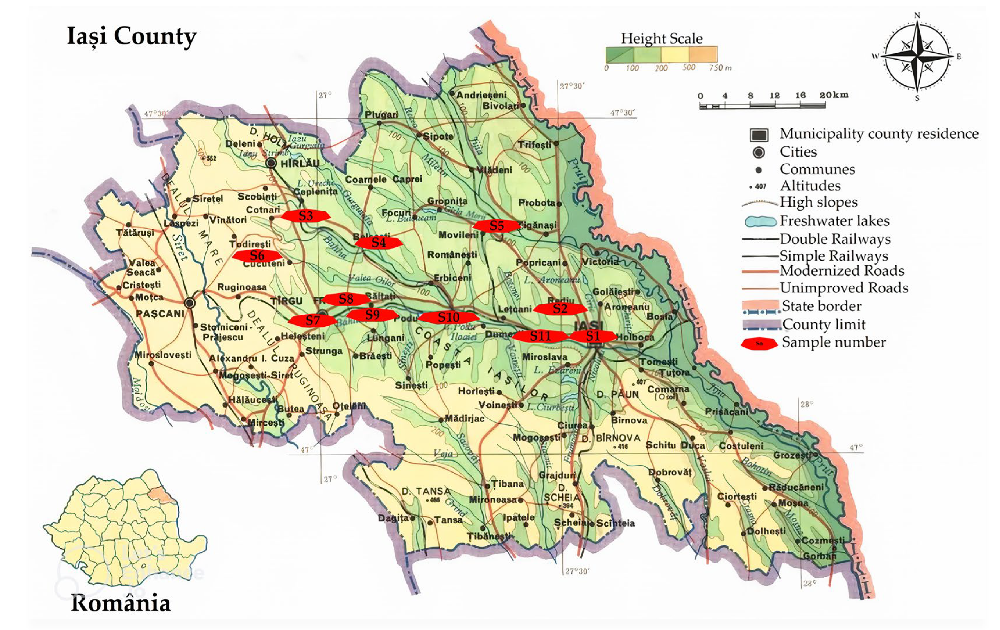
Figure 1. Location map of Iași County, Romania [42].
Agriculture 15 01070 g001
Figure 2. Micro-imaging of the soil samples (1–11 show the SEM images corresponding to each analyzed soil sample) using SEM.
Agriculture 15 01070 g002
Figure 3. Scatter plots on the relation between organic carbon (a) and humus (b) proportions and Cu accumulation.
Agriculture 15 01070 g003
Figure 4. Scatter plots on the relation between Cd and organic carbon (a) and humus (b) levels.
Agriculture 15 01070 g004
Figure 5. Scatter plots on the relationship between pH and some identified metals: Hg (a); As (b); Pb (c); Ni (d); Zn (e); Co (f); Fe (g); and Mn (h).
Agriculture 15 01070 g005aAgriculture 15 01070 g005b
Figure 6. Principal component analysis (a) and the correlation matrix (b) in metals and analysed soil samples (a). H—humidity; OC—organic carbon; Hum—humus. Samples from protected areas are represented with blue.
Agriculture 15 01070 g006
Figure 7. Principal component analysis (a) and the correlation matrix (b) for pollution assessment indexes and analysed soil samples (a). H—humidity; OC—organic carbon; Hum—humus. Samples from protected areas are represented in blue.
Agriculture 15 01070 g007
Table 2. Soil types found in the samples from Iași County, according to their geographical locations.
SampleSampling PlaceDominant Economic ActivitySoil Classification [45]Geographical Location [46]
S1Adamachi FarmAgricultureChernozem47.194374518197066, 27.55311250136081
S2Mârzești ForestProtected areaChernozem47.232779486481824, 27.497558910470836
S3Cotnari WineryWinemakingChernozem and phaeozem47.36383421700579, 26.945706995006784
S4Plopi Lake, BelceștiProtected areaChernozem47.325697560359906, 27.1010127547471
S5Moldova DeltaProtected areaChernozem47.35252959717897, 27.372164884260567
S6Todirești CommuneAgriculture and animal husbandryChernozem and phaeozem47.30612296028698, 26.842769644010666
S7Orchard, Târgu FrumosHorticultureChernozem47.21392362480122, 26.96193925069864
S8Meadow, Ion Neculce CommuneAgricultureChernozem47.244195859750484, 27.053936241207516
S9Olma Orchard, BălțațiHorticultureChernozem47.223306965075466, 27.10131728108934
S10Podu IloaieiAgricultureChernozem47.218037296762404, 27.25369206666353
S11Valea lui DavidProtected areaChernozem47.191101871447884, 27.468039211982386
Table 3. Evaluation of soil pH reactions.
Values in Aqueous SuspensionReaction Type
≤3.5Strongly acid
3.51–4.30Very strongly acidic
4.31–5.00Moderately strong acid
5.01–5.40
5.41–5.80
Moderately acid
5.81–6.40
6.41–6.80
Slightly acid
6.81–7.20Neutral
7.21–7.80
7.81–8.40
Slightly alkaline
8.41–9.00Moderately alkaline
>9.01Strongly alkaline
Table 4. Physicochemical properties.
Sample Humidity (%)Organic Carbon Content (%)Humus Content (%)pHReaction Type
S117.543.435.927.395Slightly alkaline
S219.244.087.045.146Slightly acid
S319.501.632.828.075Slightly alkaline
S414.492.554.407.901Slightly alkaline
S518.354.097.067.682Slightly alkaline
S611.580.591.027.777Slightly alkaline
S714.561.773.067.324Slightly alkaline
S823.304.167.188.492Moderately alkaline
S917.084.087.046.833Neutral
S1018.122.584.457.439Slightly alkaline
S1117.413.235.587.754Slightly alkaline
Table 5. Elemental composition of soil samples (wt.%) determined with X-ray energy-dispersive spectroscopy (EDS).
SamplesCONaMgAlSiHgPbCdKCaMnFeNiCoCuZn
S15.08 ± 0.6852.86 ± 2.270.18 ± 0.071.33 ± 0.158.83 ± 0.9220.87 ± 1.090.04 ± 0.010.10 ± 0.020.18 ± 0.062.34 ± 0.271.01 ± 0.140.32 ± 0.115.14 ± 0.830.29 ± 0.080.23 ± 0.080.35 ± 0.090.36 ± 0.08
S27.35 ± 0.5559.31 ± 0.220.09 ± 0.020.99 ± 0.046.94 ± 0.4818.78 ± 1.180.02 ± 0.0030.09 ± 0.0040.09 ± 0.011.17 ± 0.080.52 ± 0.020.18 ± 0.023.26 ± 0.050.14 ± 0.010.22 ± 0.020.21 ± 0.020.25 ± 0.01
S34.71 ± 0.5850.01 ± 2.810.19 ± 0.081.53 ± 0.287.22 ± 0.6618.47 ± 2.610.12 ± 0.030.19 ± 0.040.21 ± 0.042.43 ± 0.742.73 ± 0.930.49 ± 0.049.14 ± 1.840.40 ± 0.010.48 ± 0.060.55 ± 0.030.28 ± 0.07
S48.45 ± 1.7254.55 ± 2.470.05 ± 0.020.93 ± 0.025.63 ± 0.5819.52 ± 3.100.10 ± 0.020.08 ± 0.0020.15 ± 0.031.28 ± 0.332.79 ± 0.690.37 ± 0.084.23 ± 0.860.29 ± 0.040.31 ± 0.050.40 ± 0.070.54 ± 0.08
S515.36 ± 2.7656.38 ± 1.951.28 ± 0.580.97 ± 0.045.61 ± 0.6914.24 ± 1.110.01 ± 0.0010.08 ± 0.020.09 ± 0.021.00 ± 0.081.44 ± 0.170.10 ± 0.012.73 ± 0.700.09 ± 0.0020.10 ± 0.010.14 ± 0.010.19 ± 0.01
S63.77 ± 0.6554.33 ± 3.400.67 ± 0.280.74 ± 0.099.38 ± 0.3022.23 ± 2.570.07 ± 0.020.08 ± 0.020.16 ± 0.033.90 ± 0.550.64 ± 0.060.23 ± 0.022.23 ± 0.360.28 ± 0.020.23 ± 0.030.40 ± 0.060.34 ± 0.04
S78.61 ± 1.7157.89 ± 0.290.06 ± 0.021.78 ± 0.258.48 ± 0.2915.44 ± 0.920.10 ± 0.040.07 ± 0.010.11 ± 0.021.33 ± 0.031.07 ± 0.200.22 ± 0.013.41 ± 0.340.16 ± 0.020.21 ± 0.010.29 ± 0.010.29 ± 0.02
S85.41 ± 0.1843.90 ± 2.930.31 ± 0.051.23 ± 0.057.88 ± 0.1920.96 ± 1.040.06 ± 0.010.13 ± 0.020.21 ± 0.032.34 ± 0.176.43 ± 2.070.53 ± 0.127.30 ± 1.260.56 ± 0.120.52 ± 0.120.21 ± 0.070.28 ± 0.08
S914.65 ± 3.9257.93 ± 1.230.15 ± 0.041.01 ± 0.166.13 ± 0.7115.62 ± 2.440.06 ± 0.20.11 ± 0.040.05 ± 0.011.00 ± 0.130.74 ± 0.210.08 ± 0.011.88 ± 0.330.06 ± 0.010.07 ± 0.010.10 ± 0.020.13 ± 0.01
S105.62 ± 0.4058.53 ± 0.670.05 ± 0.031.25 ± 0.118.75 ± 0.1118.67 ± 0.370.05 ± 0.010.08 ± 0.020.08 ± 0.011.60 ± 0.080.73 ± 0.060.30 ± 0.053.07 ± 0.190.19 ± 0.020.20 ± 0.010.15 ± 0.020.28 ± 0.02
S115.35 ± 1.5952.10 ± 2.812.82 ± 1.602.77 ± 1.0610.19 ± 0.6220.35 ± 3.260.11 ± 0.020.08 ± 0.010.14 ± 0.020.72 ± 0.230.45 ± 0.110.22 ± 0.043.48 ± 1.090.21 ± 0.040.18 ± 0.020.25 ± 0.030.27 ± 0.07
Table 8. Results of the geo-accumulation index.
SamplesCrMnCoNiCuZnAsCdHgPbSnMean
S10−5.08−0.3200.82−2.47−0.321.740−3.910−0.86
S2−0.97−5.08−0.4900.26−3.647.0009.028.4101.32
S30.92−0.642.950.650.62−0.361.492.870−1.101.180.78
S41.40−0.733.220.870.900.031.003.320−0.321.140.99
S51.44−0.892.860.380.79−0.370.792.420−0.910.380.63
S61.09−0.753.030.451.07−0.491.263.000−0.580.850.81
S70.79−0.692.630.380.68−0.371.342.870−1.001.090.70
S80.98−0.852.950.621.02−0.571.182.000−0.05−0,100.65
S91.61−0.782.29−0.100.42−0.580.422.420−0.450.900.56
S101.24−0.833.46−0.151.30−0.351.262.745.06−0.9101.17
S112.05−0.712.880.850.79−0.411.341.740−0.581.280.84
Mean0.96−1.552.310.360.79−0.871.522.281.29−0.130.61-
Max2.05−0.643.460.871.300.037.003.329.028.411.28-
Min−0.97−5.08−0.49−0.150.26−3.64−0.3200−3.91−0.10-
Disclaimer/Publisher’s Note: The statements, opinions and data contained in all publications are solely those of the individual author(s) and contributor(s) and not of MDPI and/or the editor(s). MDPI and/or the editor(s) disclaim responsibility for any injury to people or property resulting from any ideas, methods, instructions or products referred to in the content.

