Water-Salt Thresholds of Cotton (Gossypium hirsutum L.) under Film Drip Irrigation in Arid Saline-Alkali Area

Abstract

Crop models are valuable tools for exploring the responses of crops to changes in environmental factors, and have been widely used to analyze the response of crops to varying soil water content and salinity levels in extreme drought and high salinity conditions. To obtain suitable water-salt thresholds and the total irrigation amount for cotton in the arid oasis of southern Xinjiang, the AquaCrop model was calibrated and validated using measured data from 2020 and 2021 (total irrigation amount: 255–480 mm; initial soil salinity levels: 0.2–0.6%). With the same initial soil water content, when the initial soil salinity < 7 dS/m, cotton yield did not significantly change under different levels of total irrigation amount, while when the initial soil salinity was 10 dS/m, there was a significant difference in cotton yield with a total irrigation amount > 300 mm. The total irrigation amount of 375 mm is the threshold for cotton at the low-salinity treatment, while it increases to 450 mm at the high-salinity treatment. Based on cotton performance with the AquaCrop model, the threshold values of soil salinity were 7, 9.3, 8.2 and 9.3 dS/m (EC_e) during the cotton stage of seedling, squaring, flower-boll and maturity, respectively. The total irrigation amount of 450 to 500 mm could achieve a win-win scenario for both cotton yield and water use efficiency under sandy loam soil. In summary, this study can serve as a reference for regulating water and salt in arid saline-alkali regions.

1. Introduction

Global freshwater resources are being consumed rapidly with the growth of the world population, agricultural scale and industrialization development. The diminishing global water availability has reduced crop productivity in arid and semi-arid regions [1]. In addition, the reduction of irrigation water increases the risk of soil salinization [2,3], which has gradually become a serious problem affecting the sustainable use of global agriculture and land resources [4,5]. Globally, 833 million hectares of agricultural land are affected by soil hazards of salinization [6]. It is imperative to explore the effects of water and salt stress on crops to optimize irrigation management and improve crop productivity [7,8,9,10]. However, field trials are usually time-consuming and expensive, and the results obtained cannot directly reflect variable farmland water–salt regulation and management. Compared to field observations, numerical simulations cost fewer human resources, material resources and time consumption, and can be analyzed for different environments, which can significantly help in improving crop and irrigation water management. Therefore, the application of crop model simulations to investigate the hydrological processes of farmland and its response to cultivation practices and climate change has become one of the main trends in current research [4,11,12,13].

A crop growth model usually refers to the logical mathematical expression of a crop growth system and its interaction with the climate and the soil systems. It can quantitatively describe the phenology, morphogenesis, material accumulation, distribution and production of a crop [14]. According to different crop species and crop growth driving principles, scientists have developed different crop models, such as WOFOST [15], EPIC [16,17], CropSyst [18,19], DSSAT [20] and APSIM [21,22], etc., which can all be used to improve crop management and optimize irrigation regimes. However, these models are very complex and require a large number of parameters, some of which are often difficult to obtain, and usually end users are not as aware and familiar with these parameters as the model developers [23], resulting in a higher cost for users to learn the model. In addition, some models are cultivar-specific and are not easily amenable for general use. To address these issues, FAO has developed a crop model that requires a relatively small number of model input parameters and performs well in terms of accuracy, simplicity and stability, i.e., AquaCrop (the software ‘AquaCrop’ is freely available, and the installation disk can be downloaded from the FAO website. In this study, AquaCrop model (version 6.1) was adopted using Windows 10) [24,25]. The AquaCrop model is a water-driven crop model, which can reflect the relationship between crop growth dynamics and water and yield in a relevant area. Compared with a radiation-driven model, one of the main advantages of the water-driven model is the opportunity to normalize the WP parameters (including evaporation requirements and atmospheric carbon dioxide concentration) in the former, so that under different spatio-temporal environments, it has greater applicability in different locations [26]. Hydrological models based on soil physics can also be used to simulate the effects of brackish water on both soil and crops. Kanzari et al. [27] used a calibrated Hydrus-1D model to simulate soil water–salt dynamic response and tomato yield under brackish water irrigation. However, it cannot simulate the continuous change of canopy cover on the time series.

Many scholars have applied the AquaCrop model to the growth prediction of various crops [28,29,30,31]. Abi Saab et al. [32] evaluated the performance of CropSyst and AquaCrop in simulating barley growth under different water and nitrogen regimes, and AquaCrop showed better performance than CropSyst under both optimal and non-optimal water supply. However, Ran et al. [33] used the experimental data of multiple maize varieties in Gansu to calibrate the parameters of the AquaCrop model, and the results showed that the simulation effect of the model was not as good as expected when the crops were subjected to severe water stress and crop senescence. The effect of salt is not considered in the above-mentioned scholars’ research. Using two years of cotton field trial data in Xinjiang, Che et al. [34] established a linear equation for soil salt and nitrogen relationships and obtained soil salinity thresholds. Tan et al. [11] and Zhang et al. [13] used 4-year cotton field data in Xinjiang and Hebei, respectively, to evaluate the AquaCrop model under the scenarios of drip irrigation and salt water irrigation, indicating that the model had acceptable reliability. In summary, many scholars have studied and discussed the reliability of the AquaCrop model, but some scholars have questioned its simulation expectations, indicating that the localization of the AquaCrop model parameters needs to be further determined. Meanwhile, some scholars have obtained salinity thresholds using field experiments, and, in this paper, we would like to investigate a simpler way of using the AquaCrop model to quickly simulate cotton growth.

Xinjiang is located in the northwest inland of China, and is a typical dry and water-deficient area with serious soil salinization problems [35]. As the main cotton-producing area in China [36,37], the local agriculture heavily relies on irrigation and soil salinity management. However, the interactive effects of irrigation and soil salinity on cotton growth and yield are not well understood, and the thresholds for soil water and salinity have not been determined. Therefore, the objectives of this study were: (1) to investigate the cotton response to different levels of soil water and salinity with AquaCrop, and (2) to determine the threshold of irrigation and soil salinity for cotton cultivation with scenario simulations using AquaCrop.

2. Materials and Method

2.1. Experimental Description

The experiment was carried out from 2020 to 2021 at the Soil and Water Conservation Monitoring Station (E81°12′12″, N40°37′23″) of the First Division of Xinjiang Production and Construction Corps, China. The station is located in Alar City on the northern edge of the Taklimakan Desert in the Tarim Basin at an altitude of 1014 m. It belongs to an extratropical arid continental desert climate zone with limited rainfall, a large day/night temperature variability, an annual precipitation of 46.7–61.2 mm, and an annual evaporation of up to 1877.5–2337.4 mm. The annual average temperature, precipitation, relative humidity, sunshine hours, pan evaporation and solar radiation are 11.3 °C, 45.7 mm, 48%, 2948 h, 2500 mm and 6000 MJ m⁻², respectively [4]. The soil texture is sandy loam, and the saturated water content, field capacity, permanent wilting point and saturated hydraulic conductivity are shown in

Table 1. Soil physical properties at the experimental site.

Depth. (cm)	Soil Texture	Saturated Water Content (cm3/cm3)	Field Capacity (cm3/cm3)	Wilting Water Content (cm3/cm3)	Soil Bulk Density (g/cm3)
0–20	Sandy loam	41	22	7	1.61
20–40	Sandy loam	41	22	7	1.60
40–60	Sandy loam	36	18	6	1.56
60–80	Sandy loam	36	18	6	1.56
80–100	Sandy loam	44	22	7	1.63

.

The soil data include soil depth and the number of layers, soil texture, bulk density (SBD), wilting water content (PWP), field capacity (FC) and saturated water content (θs) of each soil layer. Soil samples were collected at 0–20 cm, 20–40 cm, 40–60 cm and 60–80 cm with soil drills. The sampling location is shown in Figure 1; the SWC and soil salinity of each soil layer are expressed as mean values. The samples were air-dried and passed through a 2 mm sieve, and then the soil texture was determined by a laser particle size analyzer (BT-9300H, BETTERSIZE, China). Soil bulk density, field capacity and saturated water content of each soil layer were measured by the cutting ring method. The soil moisture characteristic curve was measured by the centrifugal method. The detailed soil parameters are shown in Table 1.

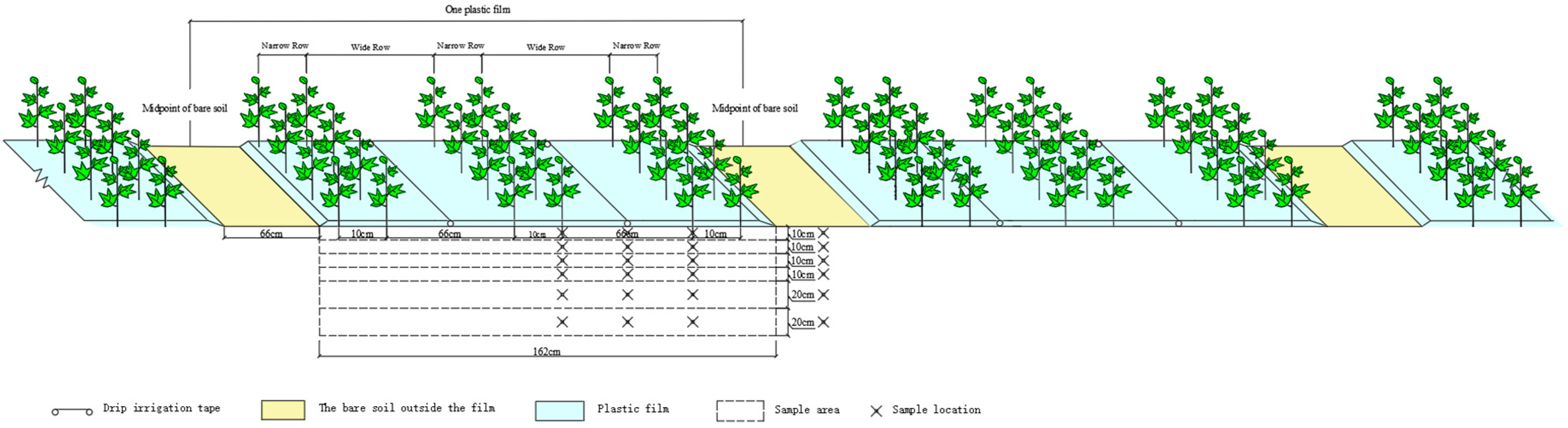
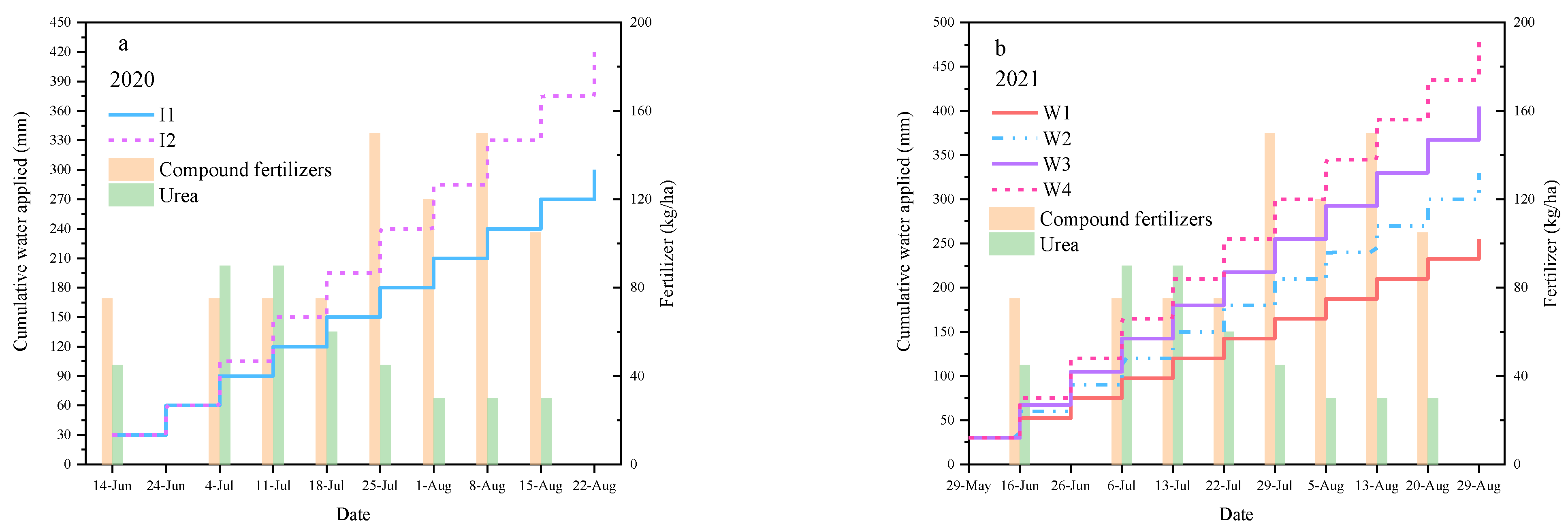
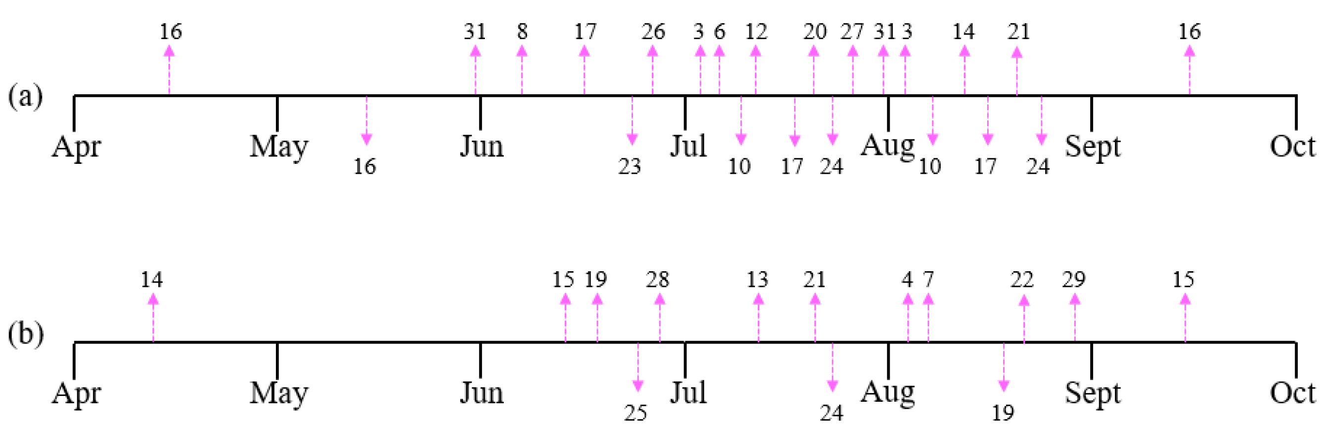
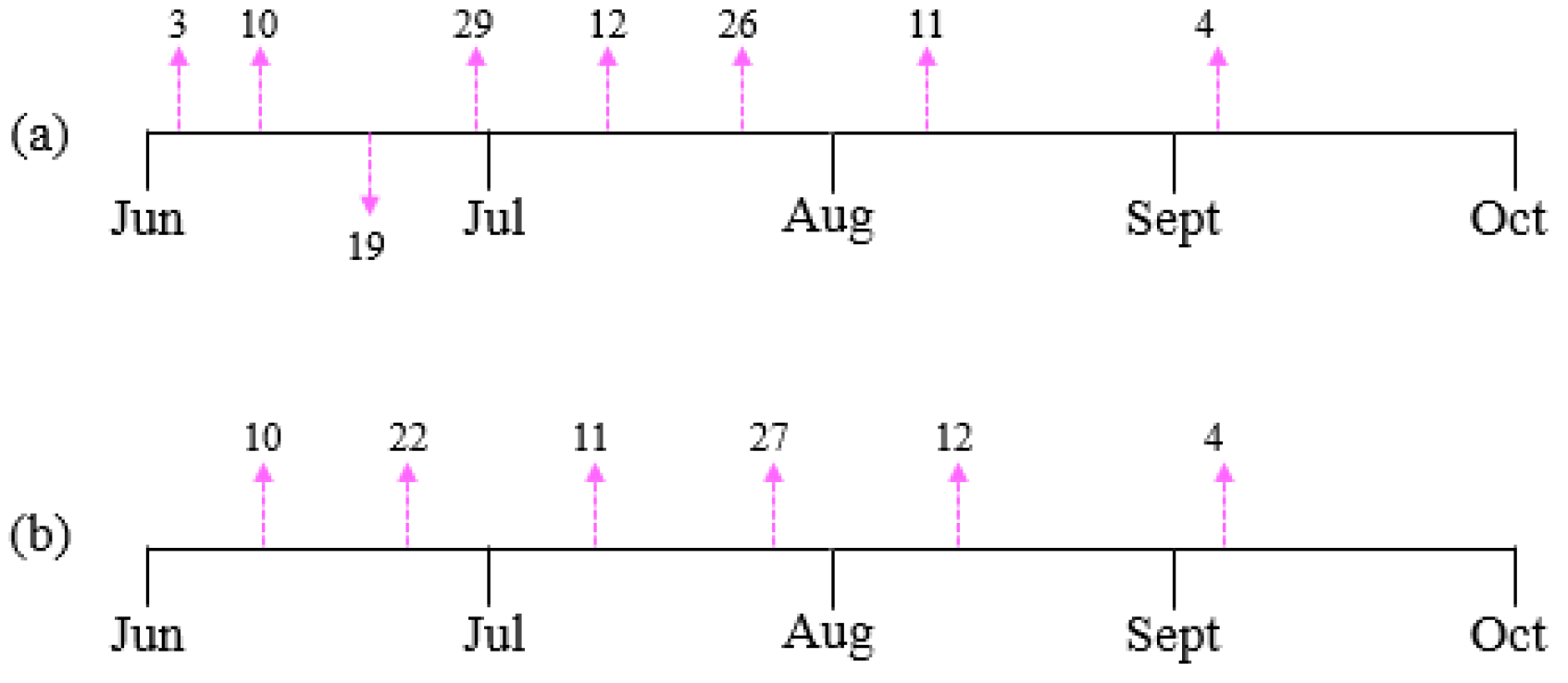
2.2. Experimental Design

The experiment consists of two factors, including salinity levels and irrigation rates. In 2020, three levels of soil salinity were designed as: 0.2% (S1), 0.4% (S2), and 0.6% (S3), respectively. The undisturbed soil in the experimental station has low salinity content (about 0.2%), which could be treated as S1. For S2 and S3, 2 g/kg and 4 g/kg of salt shells, collected from the drainage channels around the station, were mixed with the topsoil before sowing, respectively. The two irrigation rates were 30 mm (I1) and 45 mm (I2). Based on the results of the 2020 season, two irrigation levels of 22.5 and 37.5 mm were supplemented into the design for the 2021 season. The four levels were 22.5 mm (W1), 30 mm (W2), 37.5 mm (W3) and 45 mm (W4) [38]. There were 6 treatments in the 2020 season and 12 treatments in the 2021 season (Figure 2). Plots were arranged in a complete randomized grouping design with three replicates per treatment.

2.3. Agronomic Measures

The experiment dates for 2020 and 2021 were April 16 to October 10 and April 14 to October 10, respectively. The cotton variety in 2020 was Xinluzhong-27, and the variety in 2021 was Zhongmian-40, due to a variety of alternative upland cottons. Cotton was planted in a pattern of wide and narrow rows spaced 66 and 10 cm apart under film mulching, with two drip lines and six rows of cotton within each film (Figure 1) for a density of 220,000 plants/ha. The drip line was laid in the middle of the wide row with an emitter distance of 30 cm, a discharge rate of 3.0 L/h, and a working pressure of 0.1 Mpa. The experimental units were located outdoors.

Before sowing, 750 kg ha⁻¹ compound fertilizer (15% N, 15% P₂O₅, 15% K₂O) and 75 kg ha⁻¹ urea (46% N) were applied as base fertilizer. During the cotton growing season, 300 kg ha⁻¹ fertilizer (10% N, 30% P₂O₅, 10% K₂O) and 285 kg ha⁻¹ urea (46% N) were fertigated before topping, and 525 kg ha⁻¹ fertilizer (10% N, 10% P₂O₅, 30% K₂O) and 135 kg ha⁻¹ urea (46% N) were fertigated after topping (Figure 2). Weeds were controlled with herbicides from the beginning of squaring stage, and insecticides were applied according to disease and pest conditions.

2.4. Data Collection and Calculations

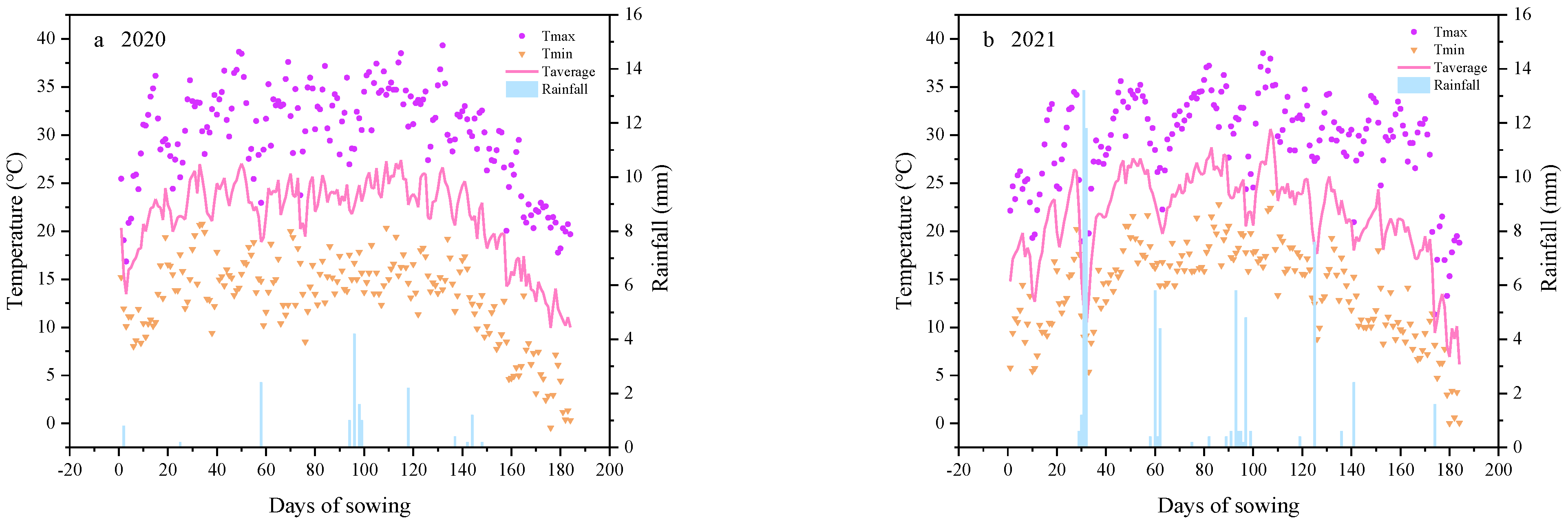
2.4.1. Meteorological Data

The meteorological data required by the AquaCrop model are minimum and maximum air temperature, reference crop evapotranspiration (ETo), rainfall and mean annual carbon dioxide concentration [40]. The air temperature and rainfall during the cotton growing in 2020 and 2021 are shown in Figure 3. The rainfall was mainly distributed in 30–140 days and 30–40 days after sowing, and the cumulative rainfall during the growth period was 15.4 mm and 64.6 mm, respectively. Most rainfall during the experiment period was ineffective (<5 mm). The meteorological data were recorded every hour by the local automatic weather station (HOBO, USA). ETo was estimated using the ETo calculator, which is a free available software developed by FAO. The ETo calculator assesses ETo from meteorological data by means of the FAO Penman–Monteith equation [41].

2.4.2. Soil Data

(Soil data) Soil conductivity (EC_1:5) was determined by measuring a 1:5 soil–water ratio mixed solution with a DDSJ-308A conductivity meter (Shanghai Instruments and Electronics Scientific Instrument, China). Soil samples were taken at depths of 10, 20, 30, 40, 60 and 80 cm. The electrical conductivity of saturated soil extracts (EC_e) was calculated with EC_1:5 as follows [42].

$$E{C}_e=8.22E{C}_{1:5}-0.33 (R^2=0.98)$$

(1)

The sampling dates for two seasons are shown in Figure 4.

2.4.3. Crop Data

(Canopy cover) To reduce transparency and simplicity for end users when using the AquaCrop model, FAO replaced the leaf area index (LAI) parameter used in most models with canopy cover (CC). The CC values in this paper were obtained by converting the LAI values. The empirical formula for canopy cover (CC) [43] was as follows:

$$CC=\frac{(1-e^{-LAI/1.3})}{(1+e^{-LAI/1.3})}$$

(2)

LAI was calculated as follows:

$$LA=L\times W\times n$$

(3)

$$LAI=LA/GA$$

(4)

where LA is the leaf area, cm²; GA is the ground area, cm²; L is leaf length, cm; W is leaf width, cm; n is the reduction factor, 0.7 [44,45].

The sampling dates for crop are shown in Figure 5. Three cotton plants were taken from each plot and were dried at 105 °C for 30 min, then dried at 75 °C to constant weight, and the dry samples were weighed. For measuring yield, three sample areas were used for each treatment, and the area of each sample area was 6.67 m². Cotton was manually picked and weighed.

2.5. Model Calibration and Validation

The AquaCrop model evolves from the K_y approach [26,46].

$$\left(1-\frac{Y}{Y_x}\right)=K_y\left(1-\frac{ET}{E{T}_x}\right)$$

(5)

where Y_x and Y are the maximum and actual yield, ET_x and ET are the maxima and actual evapotranspiration, and K_y is the proportionality factor.

Raese et al. improved the K_y approach: (1) the actual evapotranspiration (ET) became soil evaporation (E) and crop transpiration (Tr); (2) the final yield (Y) became biomass (B) and harvest index (HI) [26,46,47]. The changes described lead to the following Equations (6) and (7) at the core of the AquaCrop.

$$B=WP\times {\displaystyle \sum Tr}$$

(6)

$$Y=B\times HI$$

(7)

where Tr is the crop transpiration and WP is the water productivity parameter.

Crop production might be affected by soil salinity stress. The soil salinity stress considered by AquaCrop and its effects are presented in Figure 6 [48]. The effect of salinity stress is mainly reflected in two aspects: (1) Step 1 mainly affects canopy development, and (2) Step 2 mainly induces stomatal closure. Under the above effects, the final yield will be reduced.

The AquaCrop model consists of a meteorological module, crop module, soil module, management module and calculation module, which can simulate the dynamics of crop canopy development, biomass accumulation and yield formation. A full description of the conceptual basis and principles of AquaCrop is found in Raes et al. [26]. In this paper, the AquaCrop model Version 6.1 was used. Based on the test situation and the cotton module in the reference parameter Recommendation Manual [25], the parameters involved in the model were adjusted to make it more suitable for local conditions and various requirements.

The model was calibrated using data from the six treatments in the 2020 season, including parameters of soil, crop and management. According to the arrangement of one film, two drip lines and six rows, the film cover rate of soil was set at 70%. The phenological development time of cotton was determined by the average time of the two seasons, and the results were as follows: seedling emergence lasted for 10 days, flowering for 65 days, maximum root depth for 80 days, maximum canopy for 92 days, canopy senescence for 138 days and maturation for 171 days. The flowering and yield formation durations were 30 and 71 days, respectively. The initial soil water content and soil salinity were determined with the data obtained in the field. Calibration was carried out in Growing degree-days (GDD) mode with reference to the calibration sequence introduced by [23]: (1) Calibrate canopy cover; (2) Calibrate aboveground biomass; (3) Calibrate yield. All the simulated and measured values (SWC, Soil salinity, CC, Biomass and Yield) were within acceptable values in the six treatments in 2020.

After calibration, the model was verified using the measured data in 2021. The following statistical indexes were used to evaluate the accuracy of model calibration and validation: coefficient of determination (R²), root mean square error (RMSE) and consistency index (d). The calculation formula is as follows:

$$RMSE=\sqrt{\frac{1}{n}{\displaystyle {\sum }_{i=1}^n{(S_i-Q_i)}^2}}$$

(8)

$$R^2={\left(\frac{{\displaystyle {\sum }_{i=1}^n\left(S_i-\overline{S}\right)\left(O_i-\overline{O}\right)}}{\sqrt{{{\displaystyle {\sum }_{i=1}^n{\left(S_i-\overline{S}\right)}^2{\displaystyle {\sum }_{i=1}^n\left(O_i-\overline{O}\right)}}}^2}}\right)}^2$$

(9)

$$d=1-\frac{{\displaystyle {\sum }_{i=1}^n{\left(S_i-Q_i\right)}^2}}{{\displaystyle {\sum }_{i=1}^n{\left(\left|S_i-\overline{O}\right|+\left|O_i-\overline{O}\right|\right)}^2}}$$

(10)

where O_i and S_i are the observed and simulated values, respectively, n is the number of measured values, and O and S are the mean values of the observed and simulated values, respectively. The three statistical indicators are commonly used indicators to evaluate the performance of the model. When R² and d are closer to 1, it indicates that the prediction ability of the model is better, and the smaller the RMSE value is, the smaller the simulation error is. It has been reported that simulation results are considered acceptable if R² > 0.5 or d > 0.65 [11].

2.6. Scenario Simulation and Analysis

To obtain the optimal irrigation water amount of cotton field under different levels of soil salinity, considering the influence of initial soil moisture content, initial soil salinity and irrigation amount on cotton growth, the AquaCrop model was used to simulate the growth process of cotton during the growth period, and water use efficiency (WUE), the relative yield (Y_rel) and relative WUE (WUE_rel) were used to evaluate the response of cotton under various scenarios. Thus, the optimum irrigation amount was obtained. Upon analyzing the meteorological data in the experimental area from 1988 to 2021, the difference in local cotton reproductive periods of rainfall was small, so this study did not consider the influence of different hydrological years on cotton growth and water consumption. The groundwater depth in the station was set to 4 m. In addition, 224 scenarios were designed in this paper, including 4 levels of initial soil moisture content (0.55 FC, 0.70 FC, 0.85 FC and 1.0 FC), 8 levels of initial soil salinity (EC_e of 1, 4, 7, 10, 13, 16, 19 and 22 dS/m respectively, corresponding to EC_1:5 of 0.16, 0.53, 0.89, 1.26, 1.62, 1.99, 2.35 and 2.72 dS/m, respectively) and 7 levels of total irrigation amount (150, 225, 300, 375, 450, 525 and 600 mm, respectively). The irrigation salinity was 3 dS/m.

$$WUE=100Y/ET$$

(11)

$$Y_{rel}=Y/Y_m$$

(12)

$$WU{E}_{rel}=WUE/WU{E}_m$$

(13)

where Y is the simulated final yield (t/ha), Y_m is the simulated maximum yield (t/ha) of the initial SWC and salinity scenarios, WUE_m is the simulated maximum WUE (kg/m³) of the initial SWC and salinity scenarios, and ET is the simulated evapotranspiration (mm) throughout the growing season.

3. Results and Discussion

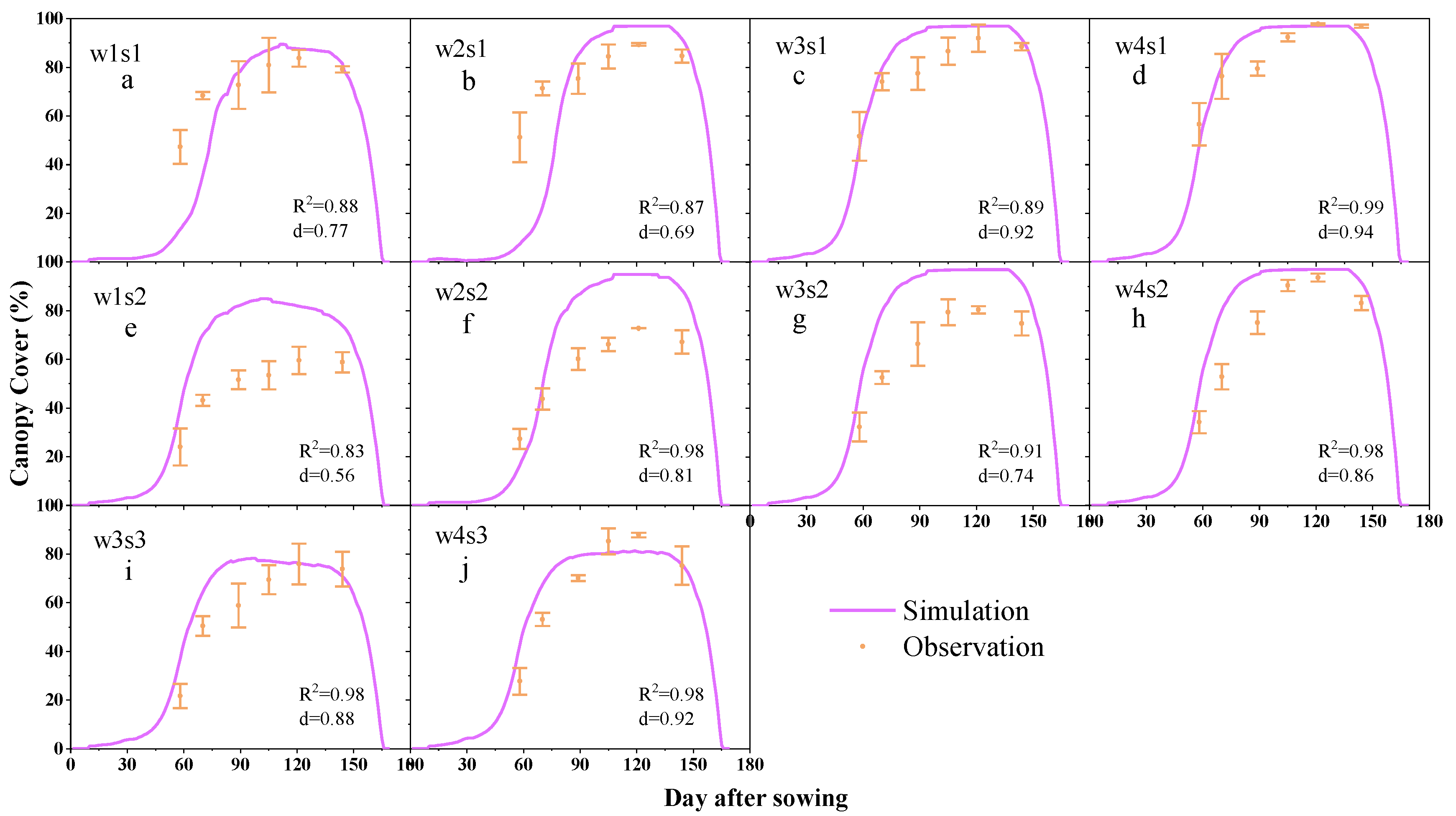
3.1. Model Calibration

AquaCrop was calibrated using data measured in 2020, and the main crop parameters in the model are shown in

Table 2. Crop parameters in AquaCrop model for cotton.

Parameter	Description	Units	Value	Remarks
CCo	Initial canopy cover	%	1.10	Calibrated
CGC	Canopy-growth coefficient	%/day	9.4	Calibrated
CDC	Canopy-decline coefficient	%/GDD	1.028	Calibrated
CCx	Maximum canopy cover	%	97	Measured
Zm	Maximum effective rooting depth	m	0.8	Measured
Zn	Minimum effective rooting depth	m	0.1	Measured
KcTR,X	Crop transpiration coefficient when complete canopy cover (CC = 1) but prior to senescence		1.10	Recommended [11,25]
WP*	Crop water productivity normalized for climate and CO2	g/m2	20	Calibrated
fyield	Reduction coefficient describing the effect of the products synthesized during yield formation on the normalized water productivity	%	72	Calibrated
HI0	Reference harvest index	%	40	Calibrated
Pexp,upper	Soil water depletion threshold for canopy expansion—Upper threshold		0.30	Calibrated
Pexp,lower	Soil water depletion threshold for canopy expansion—Lower threshold		0.65	Calibrated
fexp,w	Shape factor for water-stress coefficient of canopy expansion		1.5	Recommended [11,25]
Psto	Soil water depletion threshold for stomatal control—Upper threshold		0.35	Calibrated
fshape,sto	Shape factor for water-stress coefficient of stomatal closure		2.5	Recommended [11,25]
Psen	Soil water depletion threshold for canopy senescence—Upper threshold		0.6	Calibrated
fshape,sen	Shape factor for water-stress coefficient of early canopy senescence		2.5	Recommended [11,25]
ECen	ECe at which crop starts to be affected	dS/m	8	Calibrated
ECex	ECe at which crop can no longer grow	dS/m	35	Calibrated

. The crop model adopted the average development time of phenology from the two cotton seasons. GDD of emergence, flowering, maximum canopy and root depth, the beginning of senescence and maturity were 68, 705, 996, 926, 1755 and 2104 °C, respectively. In terms of canopy growth and development, CC₀ and CC_x were 1.10% and 97.00%; the values of CGC and CDC obtained by the change correction of the measured CC data were 9.40%/day and 1.028%/GDD, respectively, which were higher than the recommended values in the reference manual [25], which was due to different crop species and climatic conditions. The values of WP*, HI₀ and Kc_TR,X were 20 g/m², 40% and 1.10, respectively; these three parameters were all within the recommended range of the manual, and were similar to prior findings [11,13,49]. In terms of water stress, the soil moisture thresholds for canopy expansion, stomatal conductance, and canopy senescence were lower than those recommended in the parameter manual, which could be attributed to drip irrigation and mulching. For salinity stress, the EC_en and EC_ex of cotton were adjusted to 8 dS/m and 35 dS/m, respectively. The measured soil and crop data of the six treatments in 2020 were used to correct the model. The results are shown in

Table 3. Calibration of the AquaCrop model with the data set in the 2020 cotton season.

Indicator	Treatment	n	R2	RMSE	d
Soil water content	All data	138	0.98	3.21%	0.76
Soil salinity	All data	126	0.92	5.77 dS m−1	0.51
Canopy cover	All data	48	0.94	17.93%	0.78
Aboveground biomass	All data	36	0.94	1.73 t ha−1	0.96
Yield	All data	6	0.99	0.44 t ha−1	0.70

Note: n—Number of samples, R²—Coefficient of determination, RMSE—Root mean square error, d—Wilmott’s index of agreement.

, with R² > 0.92 and d > 0.7, indicating a good effect. However, its applicability needs to be verified with the measured data in 2021.

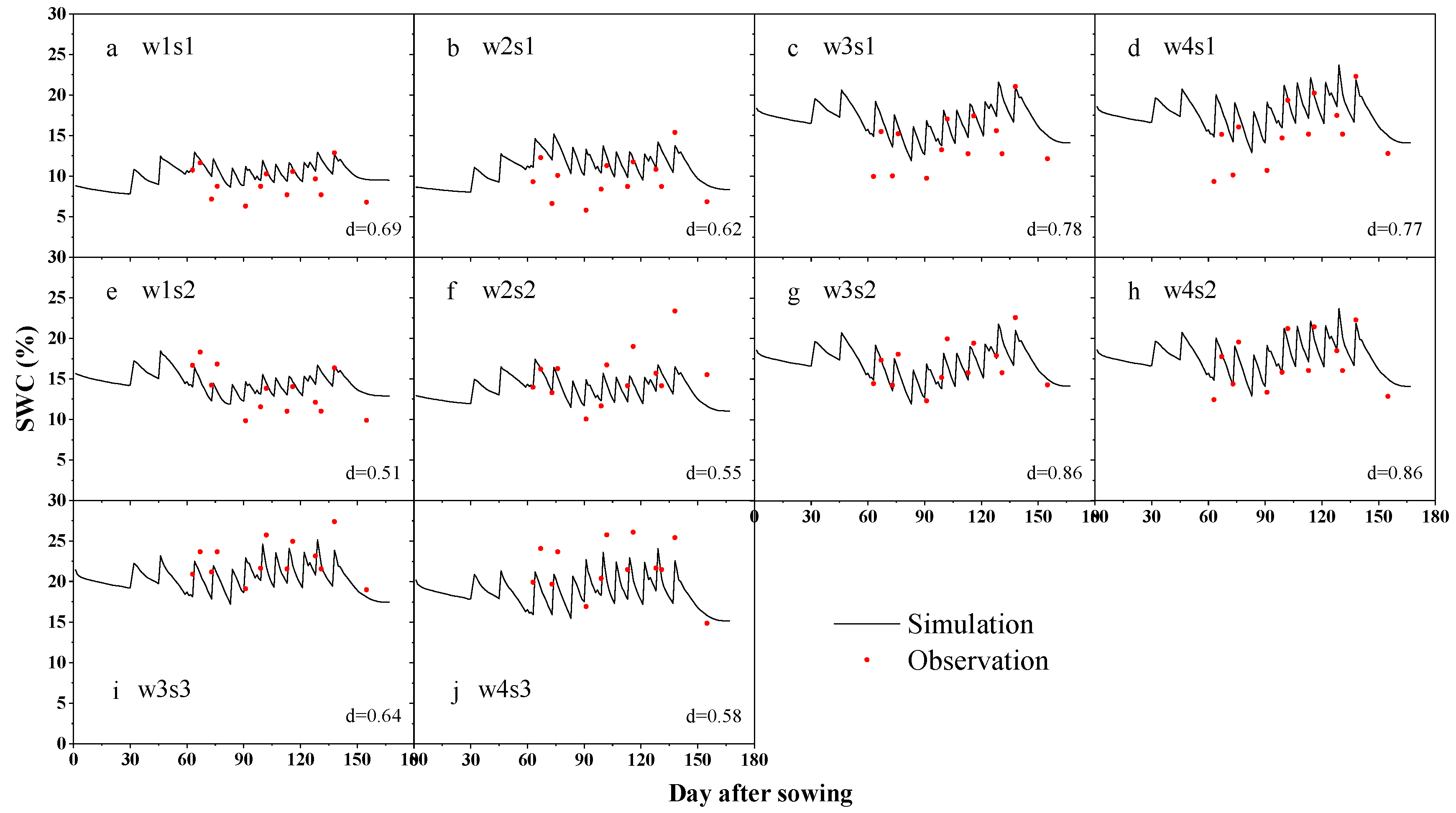
3.2. Model Validation

3.2.1. Canopy Cover

The simulation of CC with AquaCrop in the 2021 season is presented in Figure 7 and the error analysis is shown in

Table 4. Evaluation of the AquaCrop model for simulating soil water content (SWC), soil salinity, canopy cover (CC), aboveground biomass, and yield with the data set in the 2021 cotton season.

Indicator	Treatment	n	R2	RMSE	d
Soil water content	All data	130	0.97	2.88%	0.88
Soil salinity	All data	130	0.92	3.39 dS m−1	0.91
Canopy cover	All data	60	0.96	17.95%	0.81
Aboveground biomass	All data	60	0.96	2.30 t ha−1	0.94
Yield	All data	10	0.99	0.74 t ha−1	0.93

Note: n—Number of samples, R²—Coefficient of determination, RMSE—Root mean square error, d—Wilmott’s index of agreement.

. R², RMSE and d of CC simulation were 0.96, 17.95% and 0.81, respectively, indicating that the simulated CC was close to the measured value and the error was small, which could describe the variation trend of CC in the growth period under local irrigation and planting patterns. In Figure 7a,b, the simulated values of CC during the cotton rapid growth period (40–70 days after sowing) were lower than the measured values, which may be due to the lack of a soil temperature compensation module in the model, and the significant influence of film mulching on soil temperature. The increased soil temperature by film mulching can effectively accelerate the development process of the crop growth period, especially at the seedling stage [45]. Moreover, the initial SWC in W1S1 and W2S1 was low, so the simulated phenological stage was later than the actual development of cotton, and the simulated CC was less than the measured value. The simulated values of Figure 7e,f, and g were greater than the measured values in the middle stage of canopy development, similar to the study of Katerji et al. (2013) and Tan et al. (2018). The results indicated that under the condition of moderate water and salt stress, the model overestimated canopy cover. The reason may be that the maximum crop coefficient (KC_Tr,M = 1.10) given in the crop module adopts the recommended value [25] without corresponding calibration. In summary, the simulation suggested that the model’s sensitivity to water and salt stress in the vegetative growth stage needs further optimization [11,33].

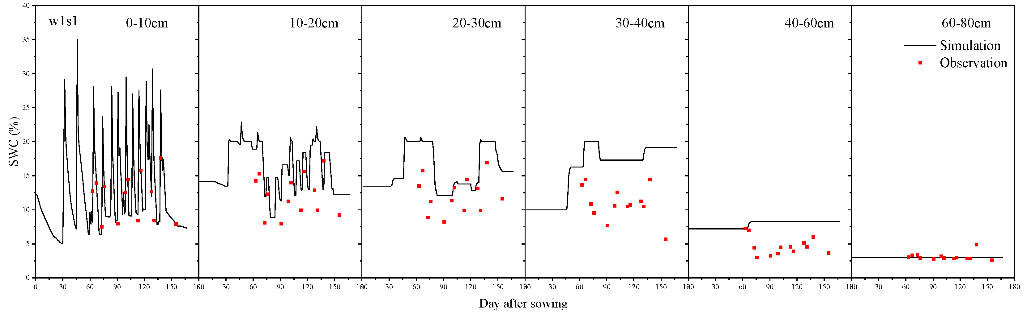
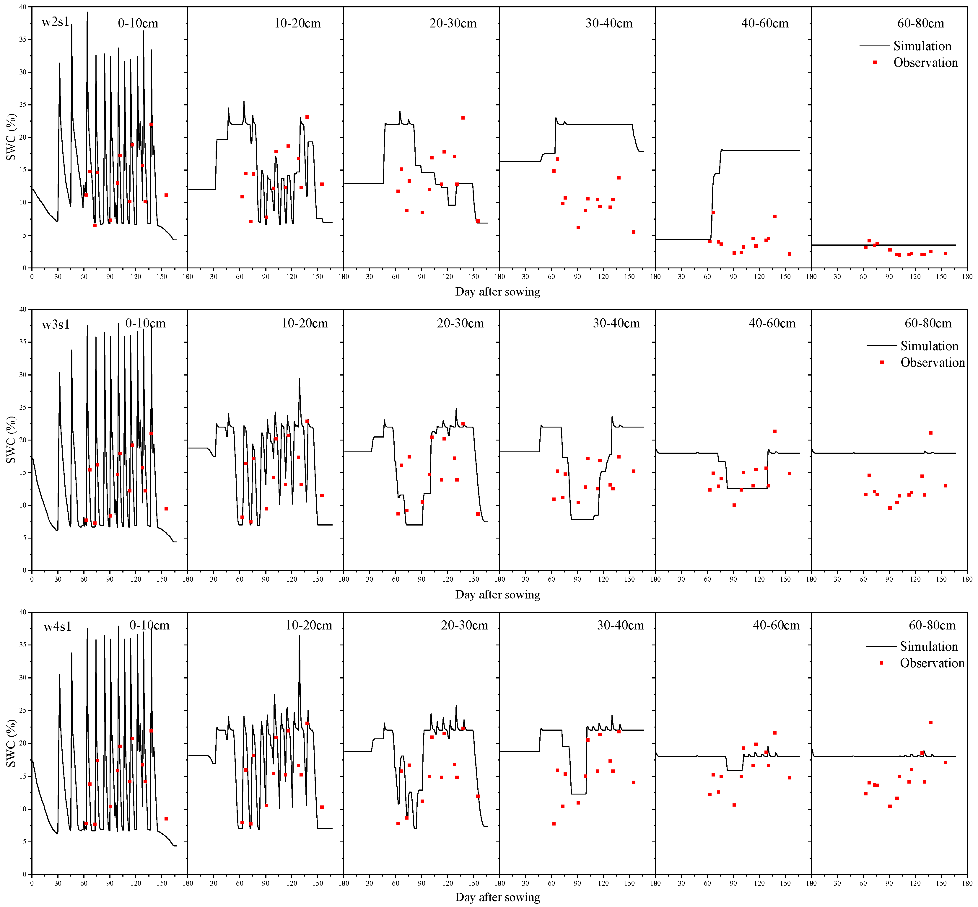
3.2.2. Soil Moisture Content

The simulation results of SWC are shown in Figure 8 and the error analysis results are shown in Table 4. R², RMSE and d were 0.97, 2.88% and 0.88, respectively, which were within the acceptable range of model simulation. The model overestimated SWC slightly, especially for W1S1, W2S1, W3S1, and W4S1 (Figure 8a–d). To further explain the difference, the seasonal changes of SWC in each soil layer of 0–80 cm depth were analyzed and are shown in Figure 9. The simulated SWC in the soil layer of 0–10 and 10–20 cm was acceptable compared to the measured values, while the simulated SWC values below the 20 cm soil layer were higher than the measured values (0–20 cm: d > 0.55; else: d < 0.55). The differences in SWC between simulated and measured values were increased with the decrease in irrigation rate. This was similar to the results of a prior AquaCrop simulation [11,13,33]. The reason for the above discrepancy may be that AquaCrop has a simplistic representation of root development, as the root growth model only includes development time and maximum effective root depth. Although the effects of water stress on root development have been considered, drip irrigation under film would increase the variability of root distribution, leading to an underestimation of root development in the model [11,50]. In addition, the spatial variability of soil in the experimental area may also lead to the above phenomenon.

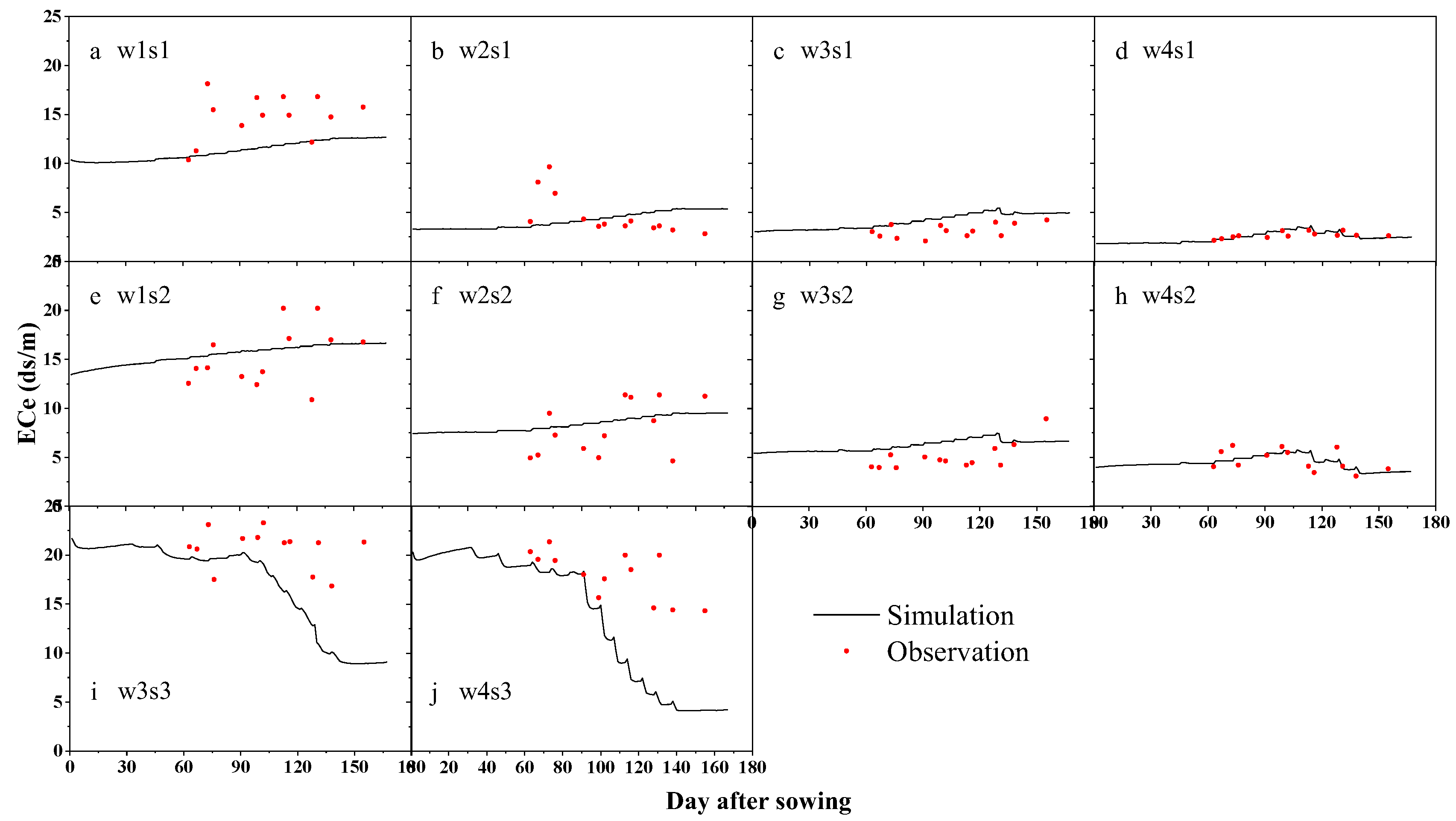
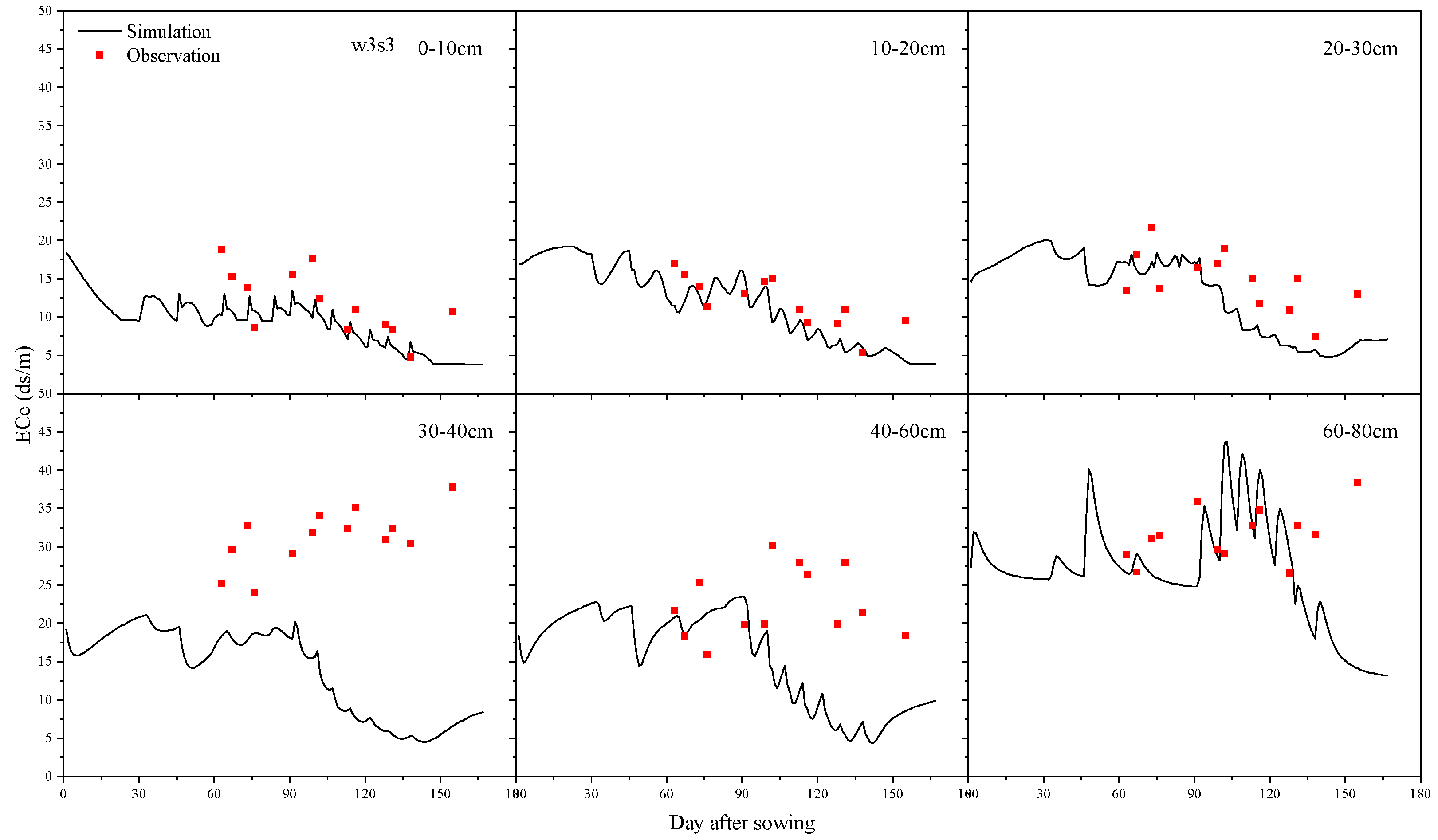
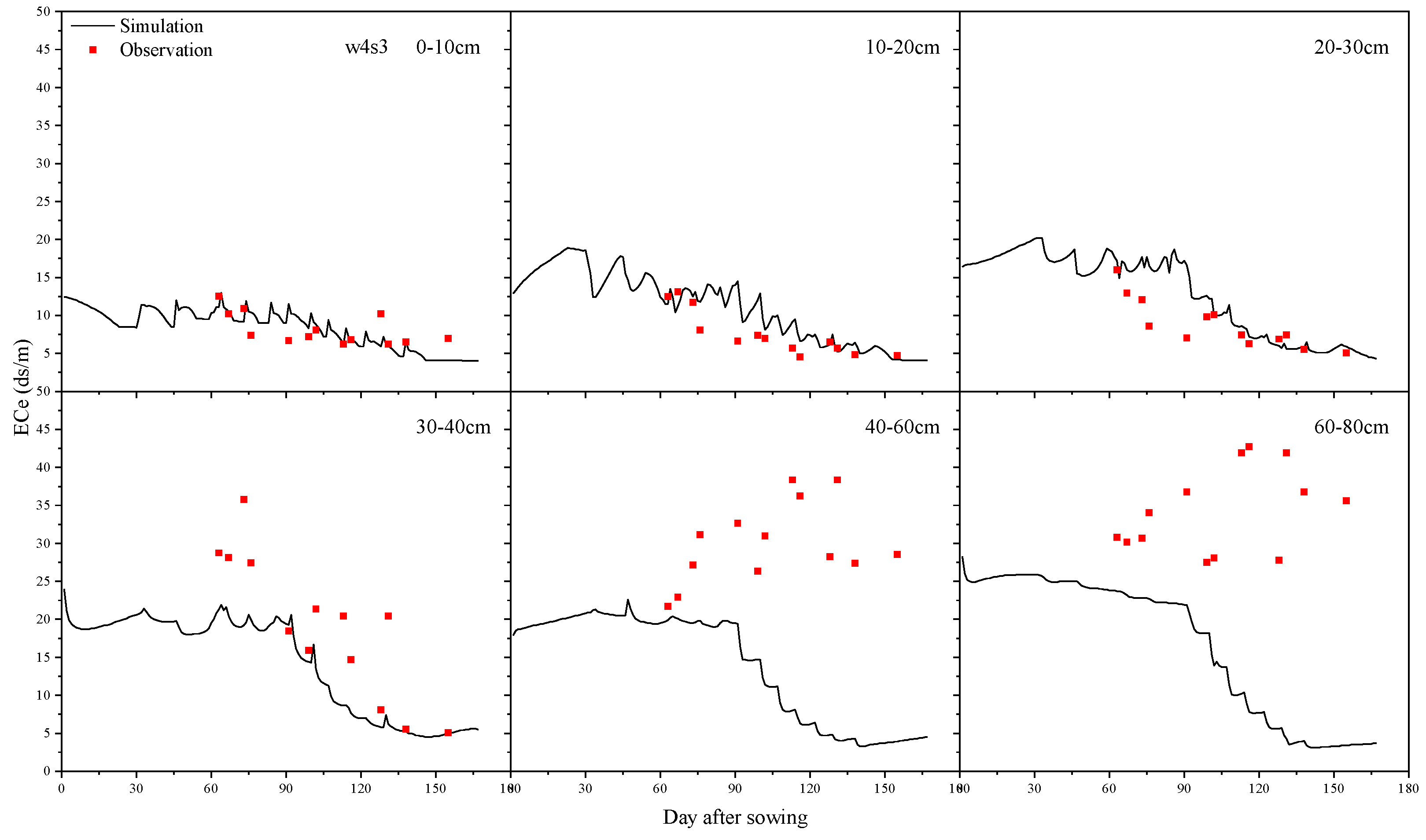
3.2.3. Soil Salinity

Although cotton is a salt-tolerant crop, the growing process and yield formation in southern Xinjiang are still affected by high salt content. The AquaCrop model was used to simulate the changes of EC_e in the 0–80 cm soil layer during the cotton growth period, as shown in Figure 10. The statistical analysis results are shown in Table 4. R², RMSE and d were 0.92, 3.39 dS/m and 0.91, respectively, which are within the acceptable range for the model simulation. The EC_e values in the 0–80 cm soil layer during the growth period were underestimated in W3S3 and W4S3, as shown in Figure 10i,j. To further explain the difference, the seasonal changes of soil salinity in each soil layer of 0–80 cm depth were analyzed and are shown in Figure 11. The simulated and measured values of EC_e in the 0–30 cm soil layer of W3S3 and W4S3 were relatively close, which can predict the changes of EC_e. However, this difference increased with the increase of soil depth (Figure 11) (0–30 cm: d > 0.6; else: d < 0.3). The reason may be that the model simulating the change of soil salinity in the root layer was too simplified. The factors affecting the solute transport in the soil profile include convection, diffusion, dispersion, adsorption and degradation, while the salinity module of the AquaCrop model only considers convection and diffusion [51]. In addition, the differences may be related to the fact that the AquaCrop model cannot effectively simulate the root development process during the growth period [11].

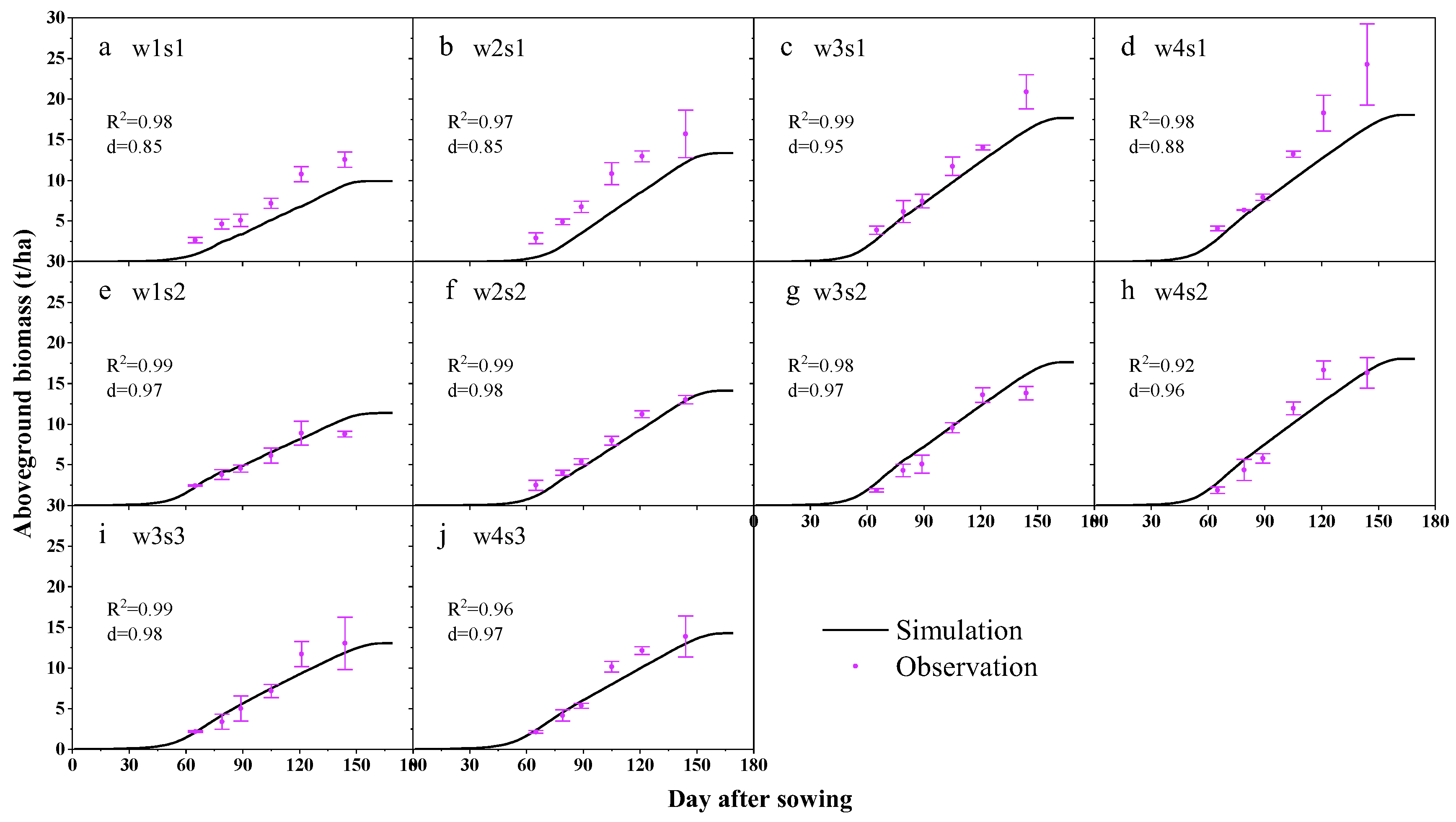
3.2.4. Aboveground Biomass and Yield

Comparison between the simulated and measured values of aboveground biomass in different treatments and the results of the statistical analysis are shown in Figure 12 and Table 4, respectively. R², RMSE and d were 0.96, 2.3 t/ha and 0.94, respectively, indicating that AquaCrop could accurately simulate the change of aboveground biomass of cotton under drip irrigation under mulch film. This was consistent with the simulation of cotton growth in southern Xinjiang, northern Greece and Hebei by AquaCrop [11,12,13]. In the late season of cotton, as shown in Figure 12a,b, the simulated aboveground biomass was slightly less than the measured value, especially for W1S1 and W2S1, which may be caused by the low WP*, because the AquaCrop model used the same WP* value to calculate biomass during the whole season. However, Ran et al. [33] and Hsiao et al. [52] suggested that the cumulative biomass could be accurately estimated by using different WP* values at different growth stages, especially in the late season. In terms of cotton yield, the comparison and statistical analysis of simulated and measured values are presented in Figure 13 and Table 4, respectively. The AquaCrop model accurately simulated cotton yield with R² of 0.99, RMSE of 0.74 t/ha, and d of 0.93. This was consistent with the results of Tan et al. [11], Jalil et al. [29] and Paredes et al. [30] on cotton, wheat and maize, respectively. Therefore, the AquaCrop model can be used to evaluate the influence of water and salt stress on cotton yield accurately.

3.3. Scenario Analysis

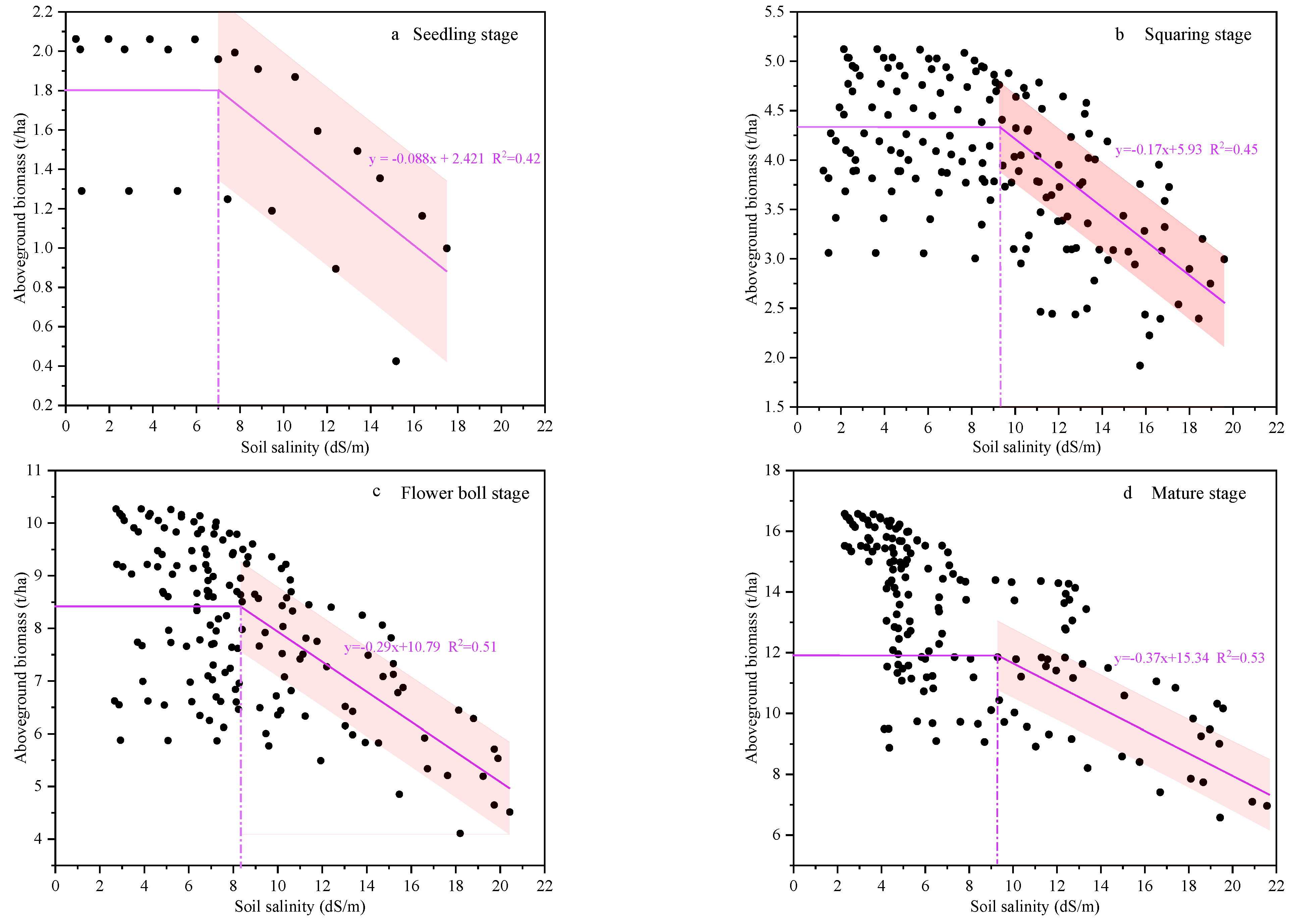
3.3.1. Response of Aboveground Biomass to Soil Salinity

The relationship between soil salinity and aboveground biomass at different growth stages is shown in Figure 14 under different scenarios. EC_e at seedling, squaring, flower boll and mature stages were 0–17.5 dS/m, 0–19.5 dS/m, 0–20.5 dS/m and 0–22 dS/m, respectively. Under low soil salinity, the aboveground biomass of cotton during the whole growing season did not change significantly under the same irrigation amount and initial SWC, ranging from 0.47 to 7 dS/m, 1.2 to 9.3 dS/m, 2.63 to 8.2 dS/m, and 2.2 to 9.3 dS/m, respectively. This was the first stage of the effect of soil salinity on the aboveground biomass. Cotton is classified as a moderately salt-tolerant crop, but salinity is still a serious threat to cotton growth, yield, and fiber quality [53]. However, several studies have shown that low salinity has no adverse effect on cotton growth [54], and that low-intensity salt stress increases bud growth, possibly due to the sparing effect of nutrients or the presence of micronutrients in the form of impurities in the saline growth medium [55]. The aboveground biomass decreased with increasing soil salinity, which was the second stage of the salt stress response function [56], and the intersection of the two stages was the salinity threshold. When the soil salinity was greater than the threshold, the relationship between the aboveground biomass and the salinity developed into a linear regression equation (the pink area in the figure was 60% of the prediction interval). The results indicated that the threshold of soil salinity at the seedling, budding, bolling and boll opening stages of cotton were 7, 9.3, 8.2 and 9.3 dS/m, respectively. The sensitivity of cotton to salt stress depends on the stage of growth and the type of salt. As the level of salinity increased, the yield of cotton decreased accordingly due to the reduction in the number of bolls and boll weight [53]. Several studies have shown that cotton germination, emergence and young seedling stage are more prone to salt stress than other stages; with the advance of the growth period, the threshold of cotton increases [57], followed by the flower and boll stages, the bud stage and the boll opening stage [58]. When the salinity exceeded the threshold, salinity significantly affected cotton growth. This was similar to the result of Che et al. [34].

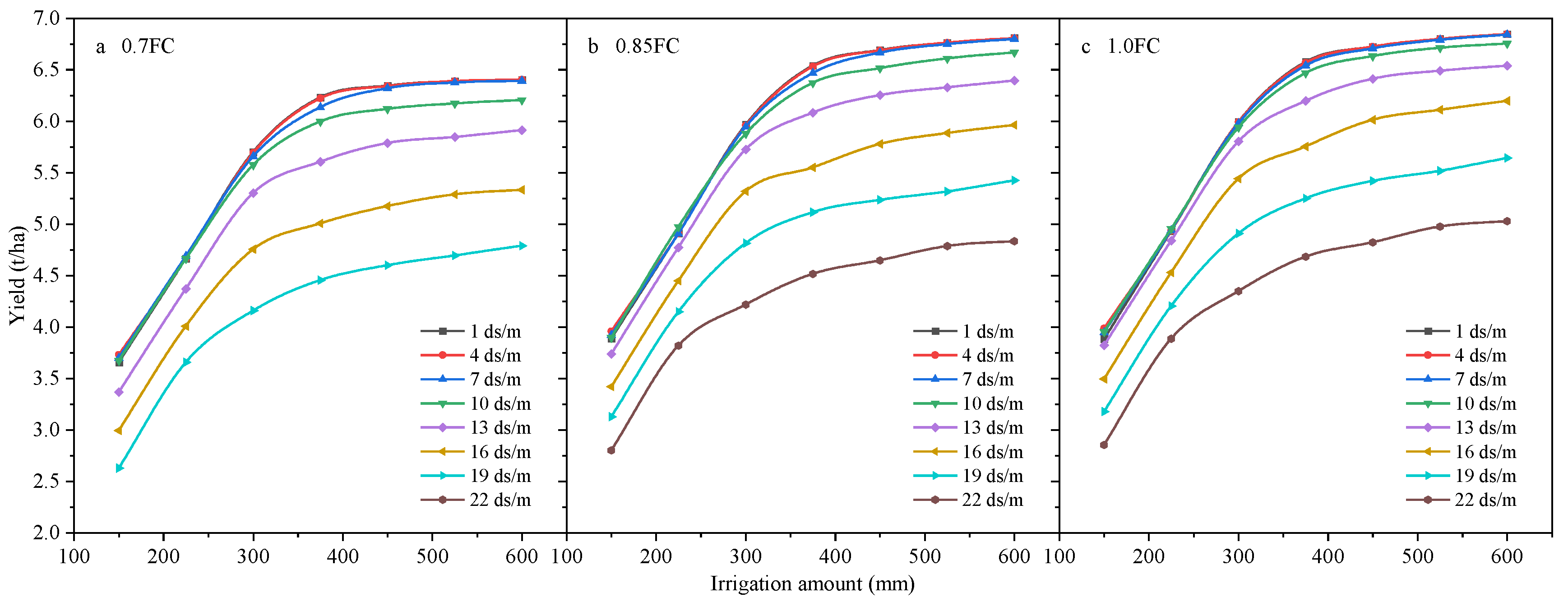
3.3.2. Cotton Yield Response to Irrigation

Cotton is not considered a drought-tolerant crop [58,59]. In the scenario simulations presented in this paper, cotton could not be grown properly with an initial soil moisture content of 0.55 FC for all scenarios with soil salinity and the initial soil moisture content of 0.7 FC with a salinity of 22 dS/m, resulting in no yield at harvesting. This was because the severe water stress and salinity stress at the seedling stage affected the emergence of cotton and the normal advancement of the phenological stage. Water and salt stress accounted for more than 50% within 15 days after sowing.

Some studies have shown that severe water stress can significantly reduce cotton yields [60]. Meanwhile, a drastic reduction in the germination percentage was observed for salinity above 10 dS/m. In response to salinity stress, the germination and emergence stages are also delayed in cotton [61,62]. At the same condition of initial soil moisture content, the yield in the treatments of the initial soil salinity of 1, 4 and 7 dS/m are robust under different total irrigation amounts (Figure 15). For the initial soil salinity <10 dS/m and the total irrigation amounts <300 mm, there was little difference in yield between the salinity treatments of 1, 4 and 7 dS/m (Figure 14a–c). When the total irrigation amounts were greater than 300 mm, the yield began to show differences between different soil salinity. The yield gap enlarged with the rise in initial soil salinity. In general, for the low soil salinity, the total irrigation amount of 375 mm was the turning point of the rapid growth period and the moderate period of each treatment, while under high salinity treatments, the corresponding irrigation amount increased to 450 mm. After that, the total irrigation amounts increased, while the yield did not increase significantly. It is not necessary to increase the irrigation amount at this point because water productivity begins to decrease [63].

When the initial soil salinity was higher than 10 dS/m, the yield decreased with increasing initial soil salinity. At the same time, under the same soil salinity, the yield under the initial water content of 0.85 FC (Figure 15b) and 1.0 FC (Figure 15c) had little difference (0–0.23 t/ha) but had a significant difference (0.23–0.86 t/ha) with that under the initial water content of 0.7 FC (Figure 15a). From the principle of calculating dry matter mass in the AquaCrop model (Figure 6), the reason was that the decrease of initial water content increased the water stress and salt stress during the whole growth period of cotton, which would reduce the development rate of CC at the seedling stage and lead to the decrease of CC_x in serious cases. In addition, water and salt stresses reduced the stomatal conductance, leading to a smaller Tr, thus reducing the dry matter quality. Therefore, reasonable initial water and salt regulation of the soil in cotton fields can moderately increase yields in the early stages of cotton growth.

3.3.3. Appropriate Irrigation Amount

Both Y_rel and WUE_rel were obtained by dividing the simulated yield and water productivity by the simulated maximum yield and water productivity, respectively. According to the simulation results in Figure 15, when the initial soil salinity was less than 10 dS/m, there was little difference in the relative yield of cotton at different total irrigation amounts. When the initial soil salinity was greater than 10 dS/m, the relative yield decreased with the increasing salinity at the same total irrigation amounts. When the initial water content was 0.85 FC and 1.0 FC, the relative yield difference was insignificant.

Therefore, values of 0.7 FC, 1.0 FC, 7 dS/m, 19 dS/m (because there is no yield at 22 dS/m under 0.7 FC) and 22 dS/m were used to analyze the changes of Y_rel and WUE_rel with irrigation quota (Figure 15). Y_rel and WUE_rel first increased and then decreased with the increase of total irrigation amounts, showing a quadratic parabolic relationship. Therefore, the intersection of the two parabolas was the optimal value for the total irrigation amount. When the initial soil salinity <10 dS/m, and the initial soil water content ≥0.70 FC, the appropriate total irrigation amount was 450 mm. For 10 dS/m ≤ the initial soil salinity ≤ 22 dS/m, the initial soil water content >0.7 FC, with a proper total irrigation amount of 500 mm. In conclusion, the appropriate total amount of drip irrigation for sandy loam cotton fields under film-mulched ranges from 450 and 500 mm. The appropriate total irrigation amounts obtained in this paper were higher than that of 240–345 mm proposed by Cai et al. [63] in Shihezi, Northern Xinjiang. These values were not that different from the total irrigation amounts of 406–462 mm obtained by Tan et al. [11] in Korla, Southern Xinjiang. The differences were related to climate, soil properties and cotton varieties.

4. Conclusions

Based on two years of data, the AquaCrop model’s performance was evaluated under different initial water contents and soil salinity in drip-irrigated cotton with film mulching in southern Xinjiang. The total irrigation amount of 375 mm was the turning point between a period of rapid yield growth and a period of slow yield growth under the low salinity treatment. The total irrigation amount under the high salinity treatment was 450 mm. The threshold values for soil water and salinity were determined using the AquaCrop scenario simulation. The results suggested that for achieving high yield and WUE of drip-irrigated cotton with film mulching, a soil salinity <10 dS/m and an initial soil moisture of 0.85 FC should be controlled, as well as the seasonal irrigation amount of 450–500 mm.

The results indicated that the model needs to be optimized for the confirmation mode of WP*, Kc_TR,X and other parameters. Considering the dynamic growth process of a crop, a fixed parameter cannot be used to represent the response of the crop at different growth stages to changes in environmental factors. At the same time, due to the complex process of salt migration and conversion in the soil, the salt module should be further improved to consider the actual situation to achieve better simulation results in water and salt simulation, since crop growth and yield formation are influenced by many factors, such as meteorological factors, cultural practices, etc. As AquaCrop has the fertilizer module, the cotton response to fertilizer should be considered in the future, to guide the irrigation management of cotton production in the region.

References

1. Mao, W.; Zhu, Y.; Wu, J.; Ye, M.; Yang, J. Evaluation of Effects of Limited Irrigation on Regional-Scale Water Movement and Salt Accumulation in Arid Agricultural Areas. Agric. Water Manag. 2022, 262, 107398. [Google Scholar] [CrossRef]
2. Devkota, K.P.; Devkota, M.; Rezaei, M.; Oosterbaan, R. Managing Salinity for Sustainable Agricultural Production in Salt-Affected Soils of Irrigated Drylands. Agric. Syst. 2022, 198, 103390. [Google Scholar] [CrossRef]
3. Poustie, A.; Yang, Y.; Verburg, P.; Pagilla, K.; Hanigan, D. Reclaimed Wastewater as a Viable Water Source for Agricultural Irrigation: A Review of Food Crop Growth Inhibition and Promotion in the Context of Environmental Change. Sci. Total Environ. 2020, 739, 139756. [Google Scholar] [CrossRef]
4. Yu, Q.; Kang, S.; Hu, S.; Zhang, L.; Zhang, X. Modeling Soil Water-Salt Dynamics and Crop Response under Severely Saline Condition Using WAVES: Searching for a Target Irrigation Volume for Saline Water Irrigation. Agric. Water Manag. 2021, 256, 107100. [Google Scholar] [CrossRef]
5. Hussain Shah, S.H.; Wang, J.; Hao, X.; Thomas, B.W. Modelling Soil Salinity Effects on Salt Water Uptake and Crop Growth Using a Modified Denitrification-Decomposition Model: A Phytoremediation Approach. J. Environ. Manag. 2022, 301, 113820. [Google Scholar] [CrossRef]
6. FAO. Mapping of Salt-Affected Soils—Technical Manual; FAO: Rome, Italy, 2020; ISBN 978-92-5-132687-9. [Google Scholar]
7. Chen, X.; Qi, Z.; Gui, D.; Sima, M.W.; Zeng, F.; Li, L.; Li, X.; Gu, Z. Evaluation of a New Irrigation Decision Support System in Improving Cotton Yield and Water Productivity in an Arid Climate. Agric. Water Manag. 2020, 234, 106139. [Google Scholar] [CrossRef]
8. Che, Z.; Wang, J.; Li, J. Effects of Water Quality, Irrigation Amount and Nitrogen Applied on Soil Salinity and Cotton Production under Mulched Drip Irrigation in Arid Northwest China. Agric. Water Manag. 2021, 247, 106738. [Google Scholar] [CrossRef]
9. Hunsaker, D.J.; Bronson, K.F. FAO56 Crop and Water Stress Coefficients for Cotton Using Subsurface Drip Irrigation in an Arid US Climate. Agric. Water Manag. 2021, 252, 106881. [Google Scholar] [CrossRef]
10. Hou, X.; Fan, J.; Zhang, F.; Hu, W.; Yan, F.; Xiao, C.; Li, Y.; Cheng, H. Determining Water Use and Crop Coefficients of Drip-Irrigated Cotton in South Xinjiang of China under Various Irrigation Amounts. Ind. Crops Prod. 2022, 176, 114376. [Google Scholar] [CrossRef]
11. Tan, S.; Wang, Q.; Zhang, J.; Chen, Y.; Shan, Y.; Xu, D. Performance of AquaCrop Model for Cotton Growth Simulation under Film-Mulched Drip Irrigation in Southern Xinjiang, China. Agric. Water Manag. 2018, 196, 99–113. [Google Scholar] [CrossRef]
12. Tsakmakis, I.D.; Kokkos, N.P.; Gikas, G.D.; Pisinaras, V.; Hatzigiannakis, E.; Arampatzis, G.; Sylaios, G.K. Evaluation of AquaCrop Model Simulations of Cotton Growth under Deficit Irrigation with an Emphasis on Root Growth and Water Extraction Patterns. Agric. Water Manag. 2019, 213, 419–432. [Google Scholar] [CrossRef]
13. Zhang, J.; Li, K.; Gao, Y.; Feng, D.; Zheng, C.; Cao, C.; Sun, J.; Dang, H.; Hamani, A.K.M. Evaluation of Saline Water Irrigation on Cotton Growth and Yield Using the AquaCrop Crop Simulation Model. Agric. Water Manag. 2022, 261, 107355. [Google Scholar] [CrossRef]
14. Hammer, G.; Cooper, M.; Tardieu, F.; Welch, S.; Walsh, B.; van Eeuwijk, F.; Chapman, S.; Podlich, D. Models for Navigating Biological Complexity in Breeding Improved Crop Plants. Trends Plant Sci. 2006, 11, 587–593. [Google Scholar] [CrossRef] [PubMed]
15. van Diepen, C.A.; Wolf, J.; van Keulen, H.; Rappoldt, C. WOFOST: A Simulation Model of Crop Production. Soil Use Manag. 1989, 5, 16–24. [Google Scholar] [CrossRef]
16. Williams, J.R. The Erosion-Productivity Impact Calculator (EPIC) Model: A Case History. Philos. Trans. Biol. Sci. 1990, 329, 421–428. [Google Scholar] [CrossRef]
17. Cabelguenne, M.; Debaeke, P.; Bouniols, A. EPICphase, a Version of the EPIC Model Simulating the Effects of Water and Nitrogen Stress on Biomass and Yield, Taking Account of Developmental Stages: Validation on Maize, Sunflower, Sorghum, Soybean and Winter Wheat. Agric. Syst. 1999, 60, 175–196. [Google Scholar] [CrossRef]
18. Stöckle, C.O.; Donatelli, M.; Nelson, R. CropSyst, a Cropping Systems Simulation Model. Eur. J. Agron. 2003, 18, 289–307. [Google Scholar] [CrossRef]
19. Stockle, C.O.; Martin, S.A.; Campbell, G.S. CropSyst, a Cropping Systems Simulation Model: Water/Nitrogen Budgets and Crop Yield. Agric. Syst. 1994, 46, 335–359. [Google Scholar] [CrossRef]
20. Jones, J.W.; Hoogenboom, G.; Porter, C.H.; Boote, K.J.; Batchelor, W.D.; Hunt, L.A.; Wilkens, P.W.; Singh, U.; Gijsman, A.J.; Ritchie, J.T. The DSSAT Cropping System Model. Eur. J. Agron. 2003, 18, 235–265. [Google Scholar] [CrossRef]
21. Keating, B.A.; Carberry, P.S.; Hammer, G.L.; Probert, M.E.; Robertson, M.J.; Holzworth, D.; Huth, N.I.; Hargreaves, J.N.G.; Meinke, H.; Hochman, Z.; et al. An Overview of APSIM, a Model Designed for Farming Systems Simulation. Eur. J. Agron. 2003, 18, 267–288. [Google Scholar] [CrossRef]
22. McCown, R.L.; Hammer, G.L.; Hargreaves, J.N.G.; Holzworth, D.P.; Freebairn, D.M. APSIM: A Novel Software System for Model Development, Model Testing and Simulation in Agricultural Systems Research. Agric. Syst. 1996, 50, 255–271. [Google Scholar] [CrossRef]
23. Vanuytrecht, E.; Raes, D.; Steduto, P.; Hsiao, T.C.; Fereres, E.; Heng, L.K.; Garcia Vila, M.; Mejias Moreno, P. AquaCrop: FAO’s Crop Water Productivity and Yield Response Model. Environ. Model. Softw. 2014, 62, 351–360. [Google Scholar] [CrossRef]
24. Foster, T.; Brozović, N.; Butler, A.P.; Neale, C.M.U.; Raes, D.; Steduto, P.; Fereres, E.; Hsiao, T.C. AquaCrop-OS: An Open Source Version of FAO’s Crop Water Productivity Model. Agric. Water Manag. 2017, 181, 18–22. [Google Scholar] [CrossRef]
25. Raes, D.; Steduto, P.; Hsiao, C.T.; Fereres, E. Reference Manual, Annexes—AquaCrop, Version 6.0–6.1, May 2018; FAO: Rome, Italy, 2016. [Google Scholar]
26. Raes, D.; Steduto, P.; Hsiao, C.T.; Fereres, E. Reference Manual, Chapter 1—AquaCrop, Version 6.0–6.1 May 2018; FAO: Rome, Italy, 2016. [Google Scholar]
27. Kanzari, S.; Daghari, I.; Šimůnek, J.; Younes, A.; Ilahy, R.; Ben Mariem, S.; Rezig, M.; Ben Nouna, B.; Bahrouni, H.; Ben Abdallah, M.A. Simulation of Water and Salt Dynamics in the Soil Profile in the Semi-Arid Region of Tunisia—Evaluation of the Irrigation Method for a Tomato Crop. Water 2020, 12, 1594. [Google Scholar] [CrossRef]
28. Maniruzzaman, M.; Talukder, M.S.U.; Khan, M.H.; Biswas, J.C.; Nemes, A. Validation of the AquaCrop Model for Irrigated Rice Production under Varied Water Regimes in Bangladesh. Agric. Water Manag. 2015, 159, 331–340. [Google Scholar] [CrossRef]
29. Jalil, A.; Akhtar, F.; Awan, U.K. Evaluation of the AquaCrop Model for Winter Wheat under Different Irrigation Optimization Strategies at the Downstream Kabul River Basin of Afghanistan. Agric. Water Manag. 2020, 240, 106321. [Google Scholar] [CrossRef]
30. Paredes, P.; de Melo-Abreu, J.P.; Alves, I.; Pereira, L.S. Assessing the Performance of the FAO AquaCrop Model to Estimate Maize Yields and Water Use under Full and Deficit Irrigation with Focus on Model Parameterization. Agric. Water Manag. 2014, 144, 81–97. [Google Scholar] [CrossRef] [Green Version]
31. Stricevic, R.; Cosic, M.; Djurovic, N.; Pejic, B.; Maksimovic, L. Assessment of the FAO AquaCrop Model in the Simulation of Rainfed and Supplementally Irrigated Maize, Sugar Beet and Sunflower. Agric. Water Manag. 2011, 98, 1615–1621. [Google Scholar] [CrossRef]
32. Abi Saab, M.T.; Todorovic, M.; Albrizio, R. Comparing AquaCrop and CropSyst Models in Simulating Barley Growth and Yield under Different Water and Nitrogen Regimes. Does Calibration Year Influence the Performance of Crop Growth Models? Agric. Water Manag. 2015, 147, 21–33. [Google Scholar] [CrossRef]
33. Ran, H.; Kang, S.; Li, F.; Du, T.; Tong, L.; Li, S.; Ding, R.; Zhang, X. Parameterization of the AquaCrop Model for Full and Deficit Irrigated Maize for Seed Production in Arid Northwest China. Agric. Water Manag. 2018, 203, 438–450. [Google Scholar] [CrossRef]
34. Che, Z.; Wang, J.; Li, J. Determination of Threshold Soil Salinity with Consideration of Salinity Stress Alleviation by Applying Nitrogen in the Arid Region. Irrig. Sci. 2022, 40, 283–296. [Google Scholar] [CrossRef]
35. Zhou, B.; Yang, L.; Chen, X.; Ye, S.; Peng, Y.; Liang, C. Effect of Magnetic Water Irrigation on the Improvement of Salinized Soil and Cotton Growth in Xinjiang. Agric. Water Manag. 2021, 248, 106784. [Google Scholar] [CrossRef]
36. Ma, K.; Wang, Z.; Li, H.; Wang, T.; Chen, R. Effects of Nitrogen Application and Brackish Water Irrigation on Yield and Quality of Cotton. Agric. Water Manag. 2022, 264, 107512. [Google Scholar] [CrossRef]
37. Yang, G.; Li, F.; Tian, L.; He, X.; Gao, Y.; Wang, Z.; Ren, F. Soil Physicochemical Properties and Cotton (Gossypium Hirsutum L.) Yield under Brackish Water Mulched Drip Irrigation. Soil Tillage Res. 2020, 199, 104592. [Google Scholar] [CrossRef]
38. Yao, B.; Li, G.; Ye, H.; Li, F. Characteristic of Spatial and Temporal Changes in Soil Salt Content in Cotton Fields under Mulched Drip Irrigation in Arid Oasis Regions. Trans. Chin. Soc. Agric. Mach. 2016, 47, 151–161. [Google Scholar] [CrossRef]
39. Wang, K.; Ma, J.; Zhou, J.; Zheng, G.; He, S. The Impacts of Irrigation Frequency on Distribution Charac-teristics of Soil Water and Salt for Salinized Cotton Soil in Southern Xinjiang. J. Irrig. Drain. 2013, 32, 118–121. [Google Scholar] [CrossRef]
40. Abedinpour, M.; Sarangi, A.; Rajput, T.B.S.; Singh, M.; Pathak, H.; Ahmad, T. Performance Evaluation of AquaCrop Model for Maize Crop in a Semi-Arid Environment. Agric. Water Manag. 2012, 110, 55–66. [Google Scholar] [CrossRef]
41. Allen, R.; Pereira, L.; Raes, D.; Smith, M.; Allen, R.G.; Pereira, L.S.; Martin, S. Crop Evapotranspiration: Guidelines for Computing Crop Water Requirements, FAO Irrigation and Drainage Paper 56. FAO 1998, 56, e156. [Google Scholar]
42. Sonmez, S.; Buyuktas, D.; Okturen, F.; Citak, S. Assessment of different soil to water ratios (1:1, 1:2.5, 1:5) in soil salinity studies. Geoderma Antarct. Soils Soil Form. Process. A Chang. Environ. 2008, 144, 361–369. [Google Scholar] [CrossRef]
43. García-Vila, M.; Fereres, E.; Mateos, L.; Orgaz, F.; Steduto, P. Deficit Irrigation Optimization of Cotton with AquaCrop. Agron. J. 2009, 101, 477–487. [Google Scholar] [CrossRef]
44. Ran, H.; Kang, S.; Li, F.; Tong, L.; Ding, R.; Du, T.; Li, S.; Zhang, X. Performance of AquaCrop and SIMDualKc Models in Evapotranspiration Partitioning on Full and Deficit Irrigated Maize for Seed Production under Plastic Film-Mulch in an Arid Region of China. Agric. Syst. 2017, 151, 20–32. [Google Scholar] [CrossRef]
45. Li, M.; Du, Y.; Zhang, F.; Bai, Y.; Fan, J.; Zhang, J.; Chen, S. Simulation of Cotton Growth and Soil Water Content under Film-Mulched Drip Irrigation Using Modified CSM-CROPGRO-Cotton Model. Agric. Water Manag. 2019, 218, 124–138. [Google Scholar] [CrossRef]
46. Doorenbos, J.; Kassam, A.H.; Bentvelsen, C.; Uittenbogaard, G. Yield Response to Water. In Irrigation and Agricultural Development; Johl, S.S., Ed.; Elsevier: Pergamon, Iraq, 1980; pp. 257–280. ISBN 978-0-08-025675-7. [Google Scholar] [CrossRef]
47. Raes, D.; Steduto, P.; Hsiao, C.T.; Fereres, E. Reference Manual, Chapter 2—AquaCrop, Version 6.0–6.1 May 2018; FAO: Rome, Italy, 2016. [Google Scholar]
48. Raes, D.; Steduto, P.; Hsiao, C.T.; Fereres, E. Reference Manual, Chapter 3—AquaCrop, Version 6.0–6.1 May 2018; FAO: Rome, Italy, 2016. [Google Scholar]
49. Wang, X.; Jiang, F.; Wang, H.; Cao, H.; Yang, Y.; Gao, Y. Irrigation Scheduling Optimization of Drip-irrigated without Plastic Film Cotton in South Xinjiang Based on AquaCrop model. Trans. Chin. Soc. Agric. Mach. 2021, 52, 293–301+335. [Google Scholar]
50. Ning, S.; Shi, J.; Zuo, Q.; Wang, S.; Ben-Gal, A. Generalization of the Root Length Density Distribution of Cotton under Film Mulched Drip Irrigation. Field Crops Res. 2015, 177, 125–136. [Google Scholar] [CrossRef]
51. Hassanli, M.; Ebrahimian, H.; Mohammadi, E.; Rahimi, A.; Shokouhi, A. Simulating Maize Yields When Irrigating with Saline Water, Using the AquaCrop, SALTMED, and SWAP Models. Agric. Water Manag. 2016, 176, 91–99. [Google Scholar] [CrossRef]
52. Hsiao, T.; Heng, L.; Steduto, P.; Rojas-Lara, B.; Fereres, E. AquaCrop—The FAO Crop Model to Simulate Yield Response to Water: III. Parameterization and Testing for Maize. Agron. J. 2009, 101, 448–459. [Google Scholar] [CrossRef]
53. Sharif, I.; Aleem, S.; Farooq, J.; Rizwan, M.; Younas, A.; Sarwar, G.; Chohan, S.M. Salinity Stress in Cotton: Effects, Mechanism of Tolerance and Its Management Strategies. Physiol. Mol. Biol. Plants. 2019, 25, 807–820. [Google Scholar] [CrossRef]
54. Khan, A.N.; Qureshi, R.H.; Ahmad, N. Performance of Cotton Cultivars in Saline Growth Media at Germination Stage. Sarhad J. Agric. 1995, 11, 643–646. [Google Scholar]
55. Kent, L.M.; Läuchli, A. Germination and Seedling Growth of Cotton: Salinity-Calcium Interactions. Plant Cell Environ. 1985, 8, 155–159. [Google Scholar] [CrossRef]
56. Zeng, W.; Xu, C.; Wu, J.; Huang, J. Sunflower Seed Yield Estimation under the Interaction of Soil Salinity and Nitrogen Application. Field Crops Res. 2016, 198, 1–15. [Google Scholar] [CrossRef]
57. Ahmad, S.; Khan, N.; Iqbal, M.Z.; Hussain, A. Salt Tolerance of Cotton (Gossypium Hirsutum L.). Asian J. Plant Sci. 2002, 1, 78–86. [Google Scholar] [CrossRef] [Green Version]
58. Wu, H.; Kang, S.; Li, X.; Guo, P.; Hu, S. Optimization-Based Water-Salt Dynamic Threshold Analysis of Cotton Root Zone in Arid Areas. Water 2020, 12, 2449. [Google Scholar] [CrossRef]
59. Penna, J.C.V.; Verhalen, L.M.; Kirkham, M.B.; McNew, R.W. Screening Cotton Genotypes for Seedling Drought Tolerance. Genet. Mol. Biol. 1998, 21, 545–549. [Google Scholar] [CrossRef]
60. Hu, M.; Tian, C.; Ma, Y. The Effect of Water and Fertilizer on Cotton Growth, Nutrition Absorption and Water Utilization. Agric. Res. Arid. Areas 2002, 20, 35–37. [Google Scholar] [CrossRef]
61. Khorsandi, F.; Anagholi, A. Reproductive Compensation of Cotton after Salt Stress Relief at Different Growth Stages. Blackwell Publ. Ltd. 2009, 195, 278–283. [Google Scholar] [CrossRef]
62. Dong, H. Genetic Improvement of Cotton Tolerance to Salinity Stress. Afr. J. Agric. Res. 2011, 6, 6798–6803. [Google Scholar] [CrossRef]
63. Cai, H.; Shao, G.; Zhang, Z. Water Demand and Irrigation Scheduling of Drip Irrigation for Cotton under Plastic Mulch. J. Hydraul. Eng. 2002, 33, 119–123. [Google Scholar] [CrossRef]
Figure 1. Planting pattern of drip-irrigated cotton with film mulching and depth of soil sampling. Spring irrigation amount of 1800 m3/ha was carried out on 8 April 2020 and 7 April 2021. Cotton seeds were sown on 16 April 2020 and 14 April 2021. The chemical topping was conducted on 18 July 2020 and 17 July 2021; defoliant (Thidiazuron) was sprayed on 24 September 2020 and 21 September 2021. The yield test was carried out on 10 October in both seasons, and the sampling range for the yield test was 2.18 m × 2.98 m (15% hectare), which was repeated three times.
Agriculture 12 01769 g001
Figure 2. Irrigation and fertilization scheduling for the 2020 (a) and 2021 (b) seasons. I1, I2, W1, W2, W3 and W4 are the different irrigation levels in 2020 and 2021, respectively. The irrigation rate was applied according to the design as shown in Figure 2. The width and length of each plot were 2.18 m and 20 m, respectively. The water source for irrigation was well water, and pressurized irrigation was used with a drip irrigation system. Water meters were installed in each plot to measure the amount of irrigation water. The designed irrigation period was 10 days for the squaring stage and 7 days for the flower boll stage [39].
Agriculture 12 01769 g002
Figure 3. The maximum temperature (Tmax), minimum temperature (Tmin), average temperature (Taverage) and rainfall during (a) 2020 and (b) 2021 seasons.
Agriculture 12 01769 g003
Figure 4. The sampling dates in 2020 (a) and 2021 (b) seasons.
Agriculture 12 01769 g004
Figure 5. The sampling dates in 2020 (a) and 2021 (b) seasons.
Agriculture 12 01769 g005
Figure 6. The relationship between salinity and crop yield. CC*: green canopy cover adjusted for micro advection; WP*: the normalized biomass water productivity.
Agriculture 12 01769 g006
Figure 7. Comparison between observed and simulated canopy cover of cotton for different irrigation and salinity treatments (aj). (The dots represent the measured data, the lines represent the simulated values, the error bars represent standard deviations. W1, W2, W3 and W4 represent irrigation amount of 22.5, 30, 37.5 and 45 mm. S1, S2 and S3 represent the soil salinity of 0.2%, 0.4% and 0.6%).
Agriculture 12 01769 g007
Figure 8. Comparison between observed and simulated average soil–water storage in the soil depth of 0–80 cm for different irrigation and salinity treatments (aj). (The dots represent the measured data, the lines represent the simulated values. W1, W2, W3 and W4 represent irrigation amount of 22.5, 30, 37.5 and 45 mm. S1, S2 and S3 represent the soil salinity of 0.2%, 0.4% and 0.6%).
Agriculture 12 01769 g008
Figure 9. Comparison between observed and simulated SWC in the 0–80 cm soil profiles for different irrigation treatments.
Agriculture 12 01769 g009aAgriculture 12 01769 g009b
Figure 10. Comparison between observed and simulated average ECe in the 0–80 cm soil profile for different irrigation and salinity treatments (aj). (The dots represent the measured data, the lines represent the simulated values. W1, W2, W3 and W4 represent irrigation amount of 22.5, 30, 37.5 and 45 mm. S1, S2 and S3 represent the soil salinity of 0.2%, 0.4% and 0.6%).
Agriculture 12 01769 g010
Figure 11. Comparison between observed and simulated ECe in the 0–80 cm soil profile for different irrigation and salinity treatments (W3S3; W4S3).
Agriculture 12 01769 g011aAgriculture 12 01769 g011b
Figure 12. Comparison between observed and simulated aboveground biomass for different irrigation and salinity treatments (aj). (The dots represent the measured data, the lines represent the simulated values, the error bars represent standard deviations. W1, W2, W3 and W4 represent irrigation amount of 22.5, 30, 37.5 and 45 mm. S1, S2 and S3 represent the soil salinity of 0.2%, 0.4% and 0.6%).
Agriculture 12 01769 g012
Figure 13. Relationship between AquaCrop on observation and simulation of cotton yield under different irrigation and salinity treatments. (The dots represent the relationship between observation and simulation).
Agriculture 12 01769 g013
Figure 14. Relationship between the aboveground biomass and the soil salinity (ECe) at different growth stages of cotton. (a, b, c and d represent the different growth stages, respectively).
Agriculture 12 01769 g014
Figure 15. Relationship between irrigation amount and cotton yield under the scenarios of initial SWC (soil water content) and soil salinity at the different FC (field capacity). (a) 0.7 FC, (b) 0.8 FC and (c) 1.0 FC.
Agriculture 12 01769 g015