Article

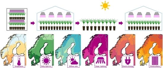
Enabling Year-round Cultivation in the Nordics-Agrivoltaics and Adaptive LED Lighting Control of Daily Light Integral

by
Marco Hernandez Velasco
1,2
1
Department of Energy and Built Environments, Dalarna University, 791 88 Falun, Sweden
2
Department of Materials Science and Engineering, Solar Cell Technology, Uppsala University, 751 21 Uppsala, Sweden
Agriculture 2021, 11(12), 1255; https://doi.org/10.3390/agriculture11121255
Submission received: 20 September 2021 / Revised: 27 November 2021 / Accepted: 8 December 2021 / Published: 11 December 2021
(This article belongs to the Special Issue Impact of Light on Horticultural Crops)

Abstract

:
High efficacy LED lamps combined with adaptive lighting control and greenhouse integrated photovoltaics (PV) could enable the concept of year-round cultivation. This concept can be especially useful for increasing the production in the Nordic countries of crops like herbaceous perennials, forest seedlings, and other potted plants not native of the region, which are grown more than one season in this harsh climate. Meteorological satellite data of this region was analyzed in a parametric study to evaluate the potential of these technologies. The generated maps showed monthly average temperatures fluctuating from −20 °C to 20 °C throughout the year. The natural photoperiod and light intensity also changed drastically, resulting in monthly average daily light integral (DLI) levels ranging from 45–50 mol·m−2·d−1 in summer and contrasting with 0–5 mol·m−2·d−1 during winter. To compensate, growth room cultivation that is independent of outdoor conditions could be used in winter. Depending on the efficacy of the lamps, the electricity required for sole-source lighting at an intensity of 300 µmol·m−2·s−1 for 16 h would be between 1.4 and 2.4 kWh·m−2·d−1. Greenhouses with supplementary lighting could help start the cultivation earlier in spring and extend it further into autumn. The energy required for lighting highly depends on several factors such as the natural light transmittance, the light threshold settings, and the lighting control protocol, resulting in electric demands between 0.6 and 2.4 kWh·m−2·d−1. Integrating PV on the roof or wall structures of the greenhouse could offset some of this electricity, with specific energy yields ranging from 400 to 1120 kWh·kW−1·yr−1 depending on the region and system design.

Graphical Abstract

1. Introduction

The climate in the Nordics (Denmark, Sweden, Finland, Norway, and Iceland) as well as in the Baltic countries (Estonia, Latvia, and Lithuania) is characterized by strong seasonal variations with short, moderately warm, and moist summers contrasted by long, very cold winters. These extreme variations considerably restrict the vegetation period, which is the time of the year when the ambient temperature stays above a certain threshold, usually of +5 °C, and allows for outdoor plant cultivation [1]. For the Nordic and Baltic countries, depending on the location, the start of the vegetation period can be delayed to halfway through spring and last just until early autumn.
Controlled environment agriculture consists in using structures that allow manipulating the indoor climate conditions and provide shelter to the crops [2]. Greenhouse cultivation allows optimizing the use of space and resources, giving protection and maintaining optimal conditions during the growth of the plants. In Northern Europe, greenhouses enable growers to cultivate their crops for longer periods and grow products locally that would have normally been imported [3]. However, this usually comes with high energy demands for heating to achieve a better indoor environment [4,5,6].
Besides the cold temperatures of the winter months, the low amounts of sunlight during this period further restrict plant cultivation in northern latitudes. While artificial lighting can be used as a remedy, using high-intensity discharge (HID) lamps to provide all the light that the plants need can result in prohibitive electricity costs and for most species, it is rarely done in practice [7,8]. Instead, the strategies adopted by growers consist of extending the day length by providing photoperiodic lighting or increasing the photosynthesis by delivering supplementary light additional to sunlight [9,10,11].
Plants use to light both as an energy source to drive photosynthesis as well as an information source with signals that trigger different processes [12,13,14]. Photosynthesis is mainly driven by photons of wavelengths between 400 nm and 700 nm. This spectral range is known as photosynthetically active radiation (PAR) [15,16]. Although the light quality, which is determined by the spectral distribution, has a strong influence on the plant’s morphology [17,18,19,20]; it is the PAR quantity that mainly affects growth and biomass production [21,22,23,24,25]. The total amount of radiation reaching the canopy is determined by the light intensity at the surface and the duration of exposure. When the photosynthetic photon flux density (PPFD, µmol·m−2·s−1) is integrated over the course of a day (photoperiod, h·d−1), the resulting daily light integral (DLI, mol·m−2·d−1) represents the accumulated PAR photons delivered on the given area during that day [26].
The DLI has proven to be a very useful and reliable tool for greenhouse cultivation, allowing growers to assess their light requirements with a simple quantity, similar to a “rain gauge” that accumulates all the PAR photons received in an area each day [27,28]. For northern latitudes where the natural light varies considerably throughout the year, the DLI can help determine the need for supplementary lighting and the strategy to use, either to reach an intensity threshold or to extend the photoperiod [29,30,31,32].
Improvements in light-emitting diodes (LED) have made them a feasible option for greenhouse lighting [33,34,35] that is economically viable [7,36] and can be adjusted to provide additional benefits for plant growth [37,38]. These new technologies have opened the possibility for new lighting strategies such as adaptive control. This consists in regulating in real-time the intensity and even the spectral output of the lamps based on the outdoor conditions to supplement only the necessary light [39,40,41,42]. This type of flexibility was not previously possible with HID lamps since they have a fixed spectral output, are usually not dimmable, and could be damaged if they are switched and cycled too often [43].
Modern artificial lights with higher efficiencies and lower heat production have also enabled the development of year-round cultivation concepts in areas where the outdoor conditions would not allow it [44,45,46,47]. LED lighting can now be used as sole-source lighting for indoor cultivation in single or multi-layered growth rooms also called vertical farms or plant factories [48,49,50,51,52,53,54]. While one of the main drawbacks of using artificial lights for plant growth is the high electricity consumption [55], renewable energy technologies such as solar photovoltaics (PV) could provide an alternative to offset some of this energy demand and produce the electricity at the place where it is needed.
Although PV essentially competes with plants for sunlight, recent years have shown an increased interest in finding ways to combine agricultural production and PV energy generation in the form of agrivoltaics [56,57]. Besides mounting PV on agricultural open fields [58,59], integrating PV directly onto the structure of greenhouses was presented as a realistic option about a decade ago [60,61,62] and since then this idea has been widely implemented in several countries [63]. This solution requires an optimization to balance the PV energy output and the crop yield [64,65,66] as well as the economic aspects [67,68], but studies have shown that it is possible to find an adequate PV roof coverage depending on the location that still allows sufficient light into the greenhouse for the plants [59,69,70].
The main goal of this work is to make a broad assessment through a parametric analysis of the potential for a year-round cultivation concept in Northern Europe using:
  • sole-source LED lighting for indoor cultivation during the winter months;
  • adaptive LED lighting control of DLI to supplement the light changes and extend the greenhouse growing season through spring and autumn;
  • an outdoor cultivation phase in the summer months;
  • greenhouses or other buildings with integrated PV to produce electricity.

2. Materials and Methods

2.1. Data Sources

To analyze these different cultivation concepts, calculations were done based on meteorological and geographical data publicly available from the European Commission Joint Research Centre in Ispra, Italy; through their online service Photovoltaic Geographical Information System-PVGIS version 5.1 [71,72]. The weather and solar radiation data source used in this study consist of a reanalysis made by the European Centre for Medium-range Weather Forecast (ECMWF-ERA-5) which includes hourly values extended between 2005 and 2016 at a spatial resolution of 0.25° for latitude and longitude forming roughly a 30 km global grid [73,74]. Despite having higher uncertainties, the ECMWF-ERA-5 dataset is the default source for the Nordic countries in PVGIS because it provides data for these regions where geostationary satellites normally have no cover.
The values were retrieved using the non-interactive service of PVGIS, using a grid cell of 0.1° × 0.1° in both latitude and longitude for the Nordic countries (except for Iceland) and the Baltics. The coordinates for this region went from 54.5° N to 70.0° N in latitude and from 4.5° E to 31.5° E in longitude: forming cells of approximately 11 km in latitude by 6 km in longitude in the south part of the region. Due to the Earth’s curvature, as the latitude increases, the distance along the longitude is reduced to 4 km per cell. When the coordinates of the requested points did not match the data points available, PVGIS’ algorithm resolved this by interpolation [75]. In total, 33,051 coordinate pairs were retrieved without counting the points over the ocean. For comparability, the cells of the geographical grid were selected with the same angular distance (0.1° × 0.1°) as those reported in similar maps for the United States [28].
A different grid was queried for Iceland since it is separated from the rest of the countries and is relatively small in comparison. The data retrieved went from 63° N to 67.5° N in latitude and from 13° W to 25° W in longitude using a cell size of 0.05° × 0.05° in both latitude and longitude. Since the values were very similar to those at the same latitudes, it was decided to present the corresponding figures for Iceland in Appendix A.
The values extracted were hourly averages of a representative day for each month. This means that for every hour of the day, the average was calculated from all the days in that month and from all years when data was available. This resulted in 24 values for each month at each point in the geographic grid (one per hour of the representative day of the month; 288 values in total for the year). The variables for which data were extracted were:
  • Global irradiance on the horizontal plane (Gh, W·m−2);
  • Direct irradiance component on the horizontal plane (Gb, W·m−2);
  • Diffuse irradiance component on the horizontal plane (Gd, W·m−2);
  • Ambient temperature calculated at 2 m above the ground (Ta, °C).

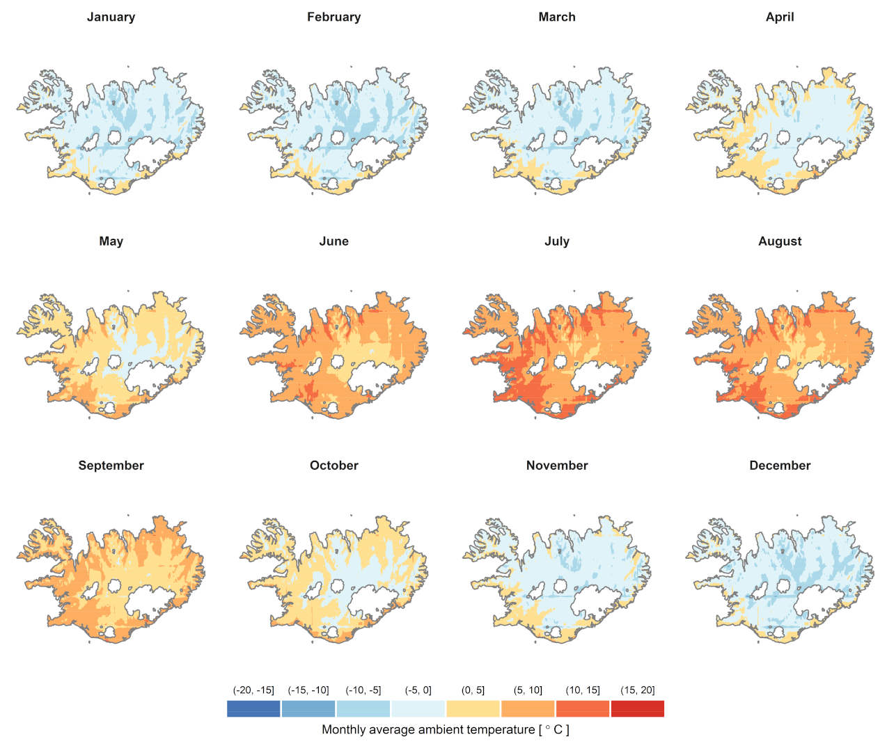
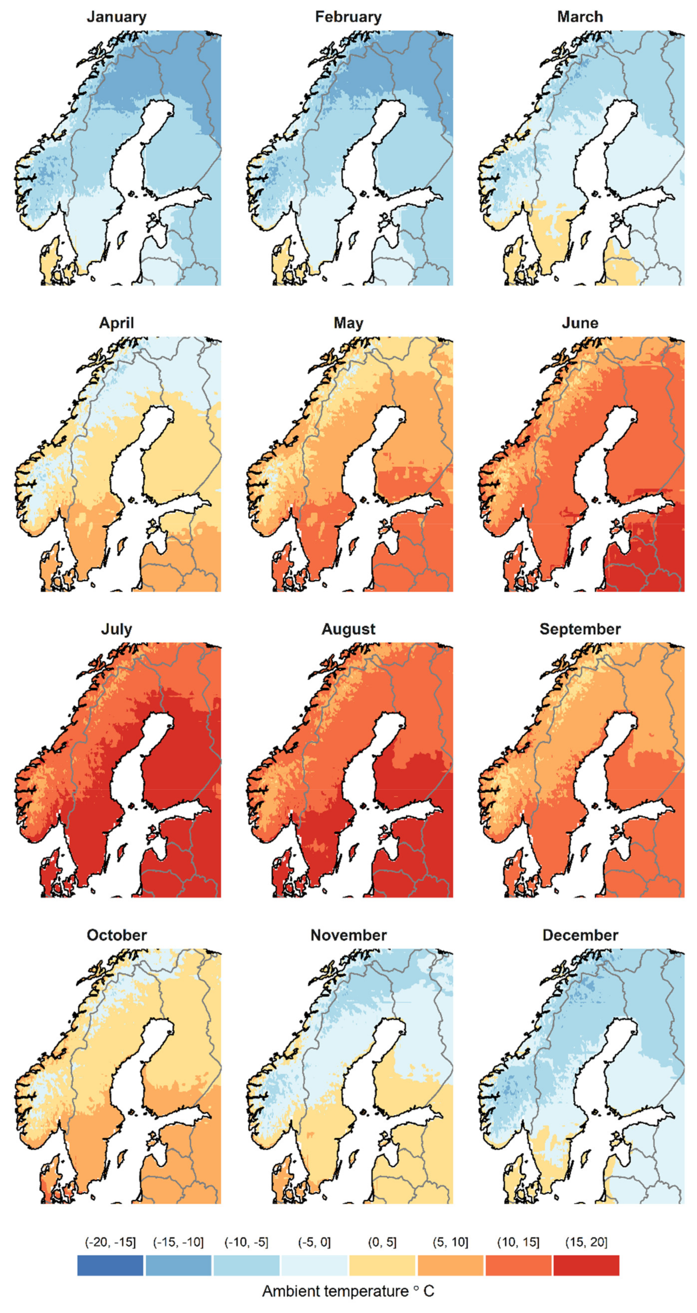
2.2. Ambient Temperature

The role of temperature in the development of plants is so important, that it allows methods like the Growing Degree Days to accurately estimate different growth stages using only the accumulation of heat units [76,77,78]. In northern climates, temperature determines the vegetation period, contributes to the cold acclimation of plants during autumn, and is one of the main cues for de-acclimation in spring together with the photoperiod [79]. Based on the monthly average ambient temperature presented in Figure 1 for the Nordic and Baltic countries (for Iceland see Appendix A, Figure A1), it was estimated that outdoor plant cultivation would be limited to the periods from [1]:
  • April to October in southern latitudes (at 55° N, about 210 days);
  • May to September in the central regions (at 63° N, about 180 days);
  • June to August in Iceland and the northernmost regions (at 70° N, about 100 days).

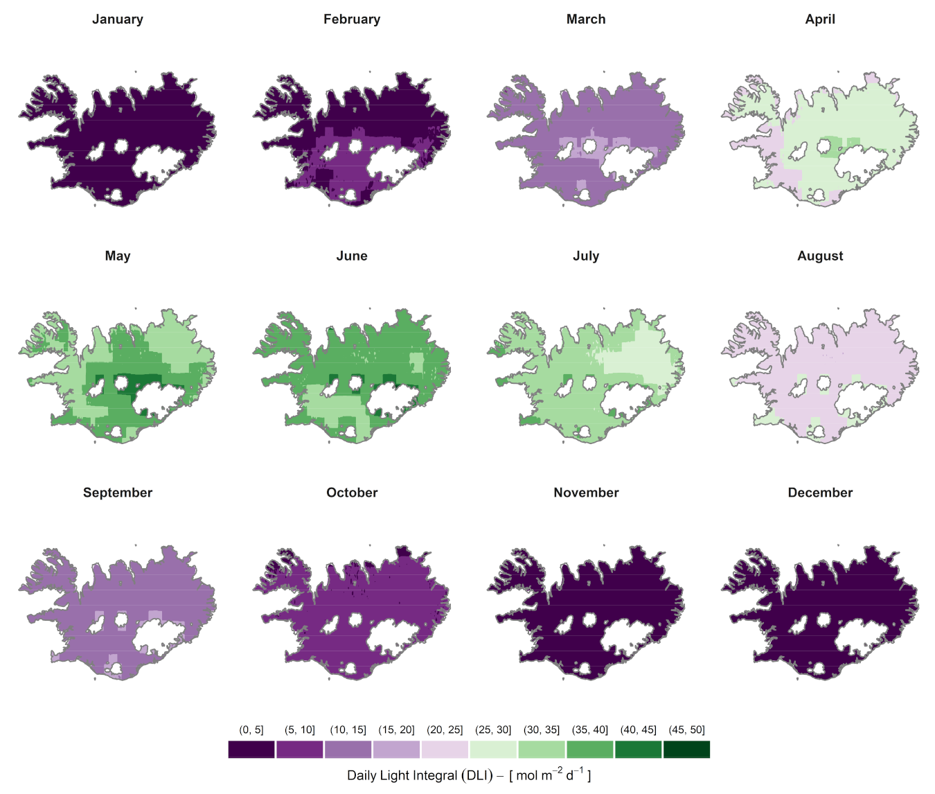
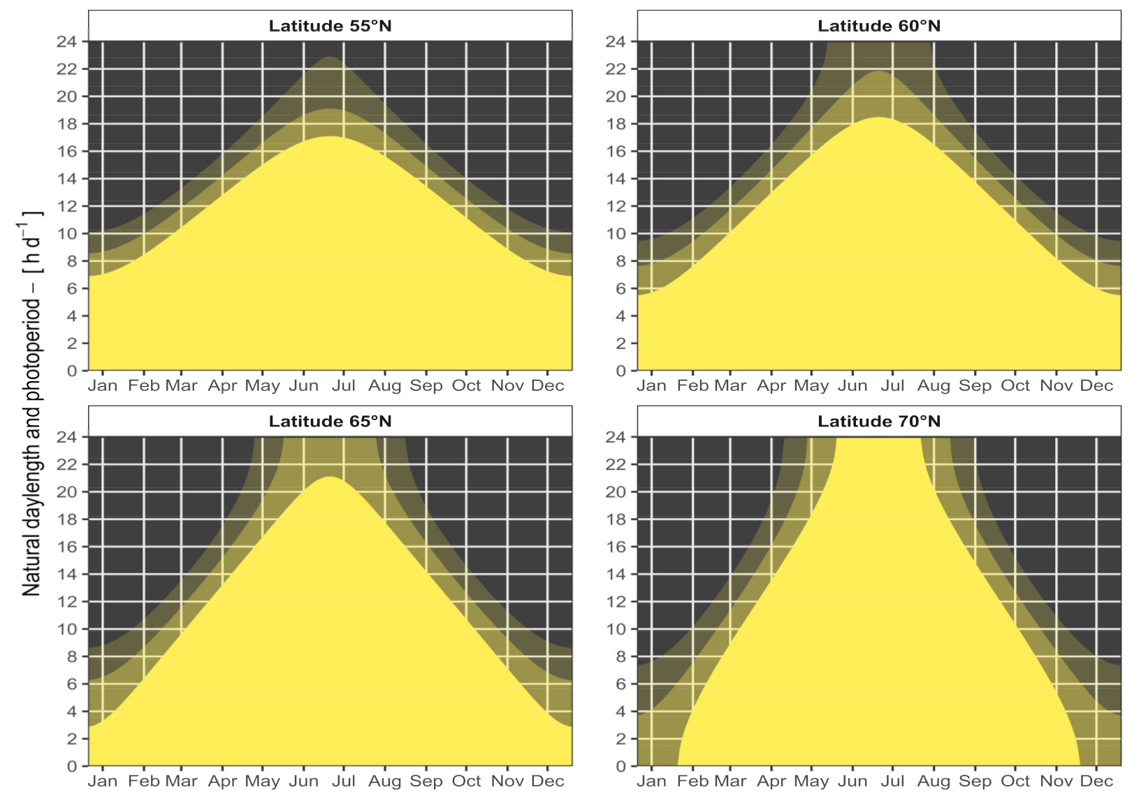
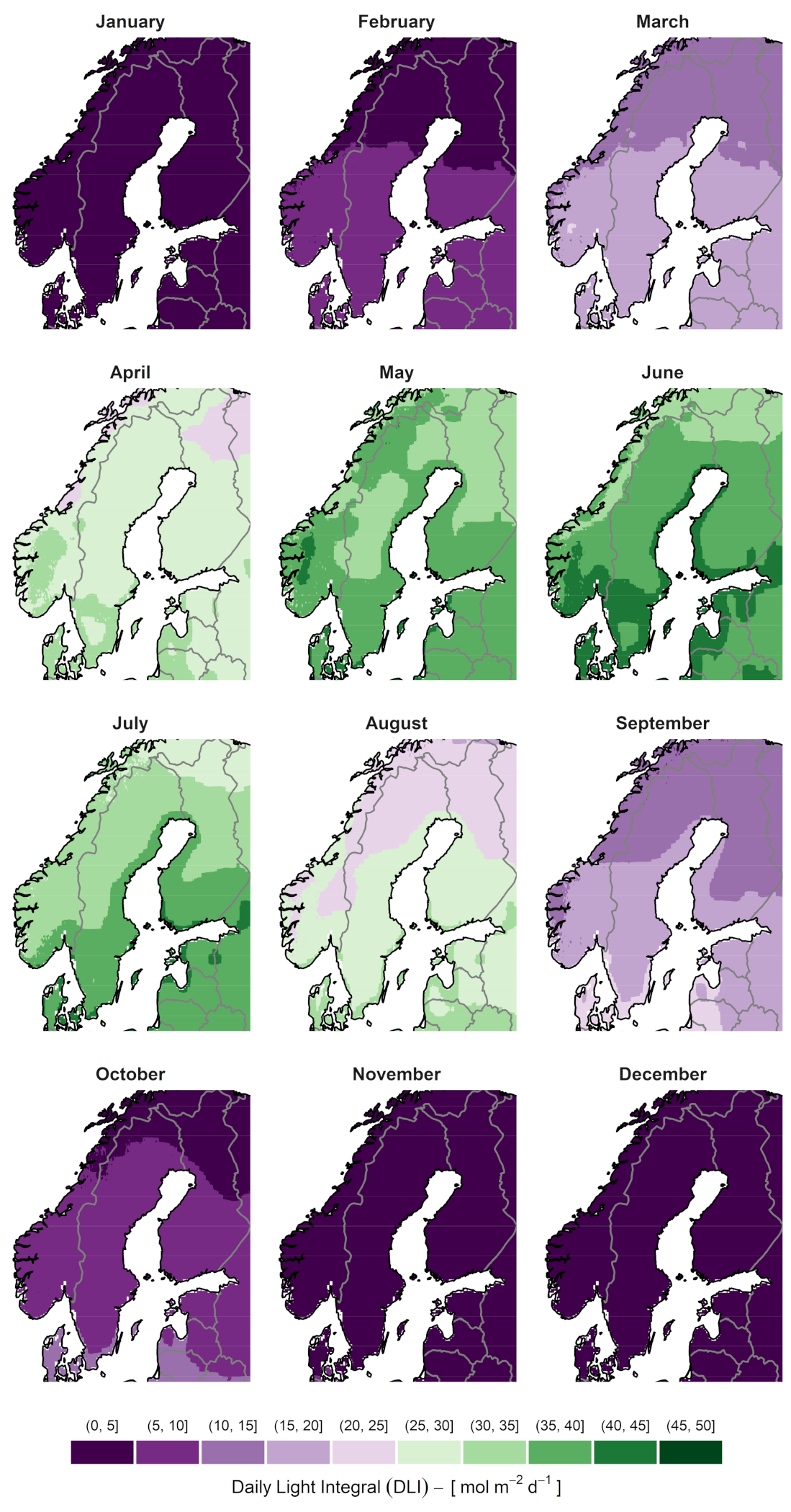
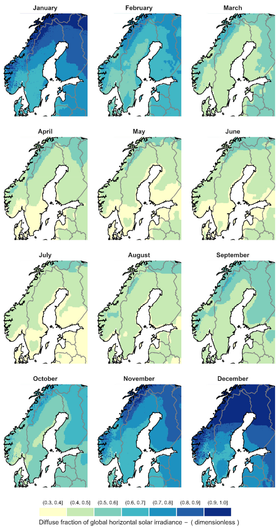
2.3. Outdoor Light Conditions

To develop a useful year-round cultivation concept, the following properties of light relevant to plant growth were analyzed: the duration of the photoperiod, the spectral composition (PAR), the intensity (PPFD), and the daily availability (DLI) [12]. Other characteristics such as light uniformity, ray direction, and intermittency might become more relevant in the future as the use of sole-source artificial lighting spreads [80].

2.3.1. Natural Daylength and Photoperiod

The seasonal differences in the duration of a day occur because of the orbital and translational movements of the Earth. These variations become more evident as the latitude increases and they are independent of changes in the global climate because they depend only on the latitude and time of the year. Plants have evolved to detect these differences in the natural photoperiod and use them as signals to adjust their development phases to the seasons and the local weather conditions [81].
Successful cultivation practices require considering the local photoperiod at the cultivation site together with the conditions at the provenance of the seeds used. Modern greenhouses and growth rooms allow to adapt and regulate the light duration by either extending the photoperiod [82,83], providing night interruption cycles [84,85], or creating short days with reduced hours of light by restricting the light [86,87,88,89,90,91].
Although most photosynthesis happens while the sun is above the horizon, plants’ photoreceptors are very sensitive and able to detect considerably small amounts of radiation (PPFD < 1 µmol·m−2·s−1). This allows them to also use the faint light before sunrise and after sunset as cues for the daily photoperiod [92]. The twilight is this illumination in the atmosphere when the sun disk is below the horizon, with civil twilight defined when the sun is 6° below the horizon and nautical twilight until 12° below [93]. Using the geometric relationships from Earth’s movements [94,95], Figure 2 shows the natural daylength together with the civil and nautical twilights for different latitudes throughout the year.

2.3.2. Estimating PPFD from Global Irradiance

All PPFD quantities presented in this work were calculated using the traditional definition of the PAR range (400–700 nm) [16]. However, research in recent years has shown that far-red photons (up to 750 nm) also contribute and influence photosynthetic activity. This suggests that updating the PAR concept towards an extended range (ePAR; 400–750 nm) might be needed as this understanding improves [96,97].
The amount of photosynthetic radiation at a place is not among the most commonly used meteorological parameters and is therefore not usually contained in standard satellite datasets. In addition, despite being relatively low-priced and easily available, quantum sensors are not normally installed in weather stations. Instead, sensors for measuring solar shortwave radiation (SWi) such as pyranometers that have a broad spectral response (normally between 280–3000 nm) are included. To use the measurements of these instruments for plant growth, numerous studies have been made in different locations to understand the relationship between PAR and SWi as well as the dependence on the atmospheric conditions and seasonal changes [98,99,100,101,102,103,104,105,106,107].
To estimate the outdoors PPFDsun from commonly reported Gh, the proportion of PAR in the SWi is needed (PAR(400–700 nm)/SWi,(280–3000 nm), unitless). Then, the amount of energy of the photons within the PAR range (EPAR, J·µmol−1) has to be measured or calculated based on the photons’ wavelengths. These two amounts can be then substituted in Equation (1) to obtain the PPFD [107]:
PPFD sun = G h PAR SW i 1 E PAR
A recent study on PAR proportion showed that if a constant of PAR/SWi = 0.45 and an EPAR = 0.223 J·µmol−1 were assumed (corresponding to the mean of the different sky conditions observed), the calculated PPFDsun deviated less than 5% from the measured value [107]. These constants can be conveniently combined with a conversion factor (0.0036 J·mol·Wh−1·µmol−1) to modify Equation (1) into a summation over 24 h to obtain the DLI (see Equation (2)) [28]. Since the average Gh values are normally reported in hourly steps, it is common to assume a constant irradiance throughout each interval.
DLI sun = t   = 1 24 G h , t · 0.0072646   mol · Wh 1
Equation (2) implies that 45% of the solar spectrum is within the PAR region and there is 0.0072646 mol of PAR photons for every Wh of SWi. Figure 3 was calculated using the Gh data extracted from PVGIS and applying Equation (2) (see Figure A2 for Iceland). The hourly radiometric data (W·m−2) was accumulated into daily quantum units (mol·m−2·d−1). This generated monthly average DLI maps with data bins of 5 mol·m−2·d−1 and a range between 0–50 mol·m−2·d−1, similar to those existing for the United States [28].
In reality, both the ratio PAR/SWi and the EPAR are not constant and depend heavily on the solar spectrum. This is in turn affected by the atmospheric conditions and the distance that light has to travel. When the sun is low in the sky e.g., at sunset or during winter, the path traveled by sunlight is longer and more photons in the PAR region are absorbed compared to those with longer wavelengths [107]. Air pollution and aerosols can also significantly scatter and attenuate the PAR irradiance [104,108]. Conversely, cloudy days with an overcast sky present a higher fraction of PAR because water vapor mainly absorbs longer wavelengths of near-infrared radiation (NIR, 760–4000 nm) [106,109].
Diffuse radiation is the light that gets scattered in the atmosphere before reaching the ground [71,94]. Figure 4 provides the monthly average diffuse fraction of global horizontal radiation (Gd/Gh) calculated from the extracted data (see Figure A3 for Iceland). Due to the influence of the atmospheric conditions on the solar spectrum, knowing the proportion of diffuse radiation in a place can be important as an indicator of the cloudiness [107] and help estimate the overall light transmittance into the greenhouse [110].

2.4. Indoor Light Conditions

During the indoor cultivation phases, either in a growth room or a greenhouse, at least part of the light would come from artificial sources. It is therefore important to define the characteristics of the lamps and the lighting control protocols planned.

2.4.1. Sole-Source Lighting

The daily output of the lamps (DLIlamps, mol·m−2·d−1) can be calculated by adding the photosynthetic light intensity at the cultivation surface (PPFDlamps, µmol·m−2·s−1) for each timestep during the photoperiod (h·d−1). Equation (3) assumes hourly timesteps and adjusts the units with a conversion factor:
DLI lamps = t   = 1 h PPFD lamps , t · 0.0036   mol · s · μ mol 1 · h 1
In a closed growth room where the light intensity is constant all day, the DLIlamps can be simply calculated by multiplying the PPFDlamps at the cultivation area by the duration of the photoperiod (h·d−1) and adjusting the units (see Equation (4)):
DLI lamps = PPFD lamps · photoperiod · 0.0036   mol · s · μ mol 1 · h 1
The efficiency of a growth lamp is measured as the ratio of the luminous power output to the electrical power input (Wlight/Wel). However, for cultivation purposes, it is more useful to compare the efficacy which is a measure of photon output rate (measured in µmol·s1) against the electrical power input (Wel). If only the PAR photons are considered, then the parameter is called photosynthetic photon efficacy (PPE, µmol·J−1) [7,54].
When the lamp efficacy measurements are done using a flat-plane integration method and assuming no other energy losses [7]; the PPE (µmol·J−1) can be used to calculate the daily electrical energy consumption (Eel, lamps, kWh·m−2·d−1) per cultivation surface. Equation (5) accounts also for the conversion from quantum to energy units:
E el ,   lamps = DLI lamps PPE · 3.6   mol · J · μ mol 1 · kWh 1
Equations (4) and (5) can then be combined into Equation (6) to calculate Eel, lamps directly from the PPFDlamps, the photoperiod, and the lamp efficacy. This can be useful to directly compare and select the best lamp for a specific growth light protocol.
E el ,   lamps = PPFD lamps · photoperiod PPE · 1000   W · kW 1

2.4.2. Greenhouse Light Transmission

The amount of outdoor light that is transmitted into a greenhouse depends in great measure on the covering material properties together with the angle of incidence at which the irradiance arrives [110]. When the light reaches the surface, it is either reflected, absorbed, or transmitted through the material [111,112]. The highest transmittance of PAR occurs when the incoming light is at 90° from the roof surface; this is called the perpendicular PAR transmittance (τp, PAR, %) [112]. However, since the position of the sun in the sky varies with time and latitude, so does the proportion of light reaching inside. A better indicator of the natural light available is the global or hemispherical PAR transmittance (τh, PAR, %) which considers the total transmission inside the greenhouse [111,112].
Due to the broad number of locations in this study, it was decided to use the assumption of a uniformly bright sky [113]. This implies that all sunlight reaching the greenhouse surface is diffuse and has the same spectrum. Thus, τh,PAR is a constant value regardless of season or roof orientation. The light inside the greenhouse (PPFDgreenhouse) was then calculated as a percentage of the outdoor PPFDsun using Equation (7) [112]:
PPFD greenhouse = τ h ,   PAR · PPFD sun
To compensate for the shortcomings of this simplification, the calculations were done for different values of τh,PAR (40%, 55% or 70%) selected to be within the range of those reported in different studies of various greenhouse materials and at various locations, obtained through simulations or from measurements [65,110,111,114,115,116,117,118].

2.4.3. Greenhouse Lighting Control Protocols

Two previously established lighting control protocols were compared in this study: an on-off control vs. an adaptive control [42]. In both cases, dimmable LED fixtures were assumed to be used to maintain a predefined minimum light level (PPFDthreshold) throughout the entire photoperiod. In the two protocols, when the natural light transmitted inside the greenhouse reached or surpassed the threshold (PPFDgreenhouse ≥ PPFDthreshold), the lamps would turn off and emit no light (PPFDlamps = 0).
With the on-off control protocol (Equation (8)), if the threshold was not reached with natural light (PPFDgreenhouse < PPFDthreshold), the lamps would then produce exactly the amount of light at the setting level (PPFDlamps = PPFDthreshold). This would be equivalent to having lamps set exactly at the PPFDthreshold and just switching them on and off. In contrast, the adaptive control protocol (Equation (9)) considers the dimmability of the LED fixtures. The output of the lamps is assumed to be continuously adjusting and regulated to provide only the necessary output to reach the desired threshold while considering the incoming sunlight (PPFDlamps = PPFDthreshold − PPFDgreenhouse).
PPFD   on off = 0 , PPFD greenhouse PPFD threshold PPFD threshold , PPFD greenhouse < PPFD threshold
PPFD   adaptive = 0 ,                                                   PPFD greenhouse PPFD threshold PPFD threshold PPFD greenhouse ,     PPFD greenhouse < PPFD threshold

2.5. Year-Round Cultivation Concept

In the proposed year-round concept, indoor cultivation in northern Europe would need to be done for at least 6 months and up to 9 months depending on the location. After evaluating Figure 1, Figure 2 and Figure 3, it was decided to consider an extreme scenario with about 3 months outdoor cultivation complemented by 9 months of indoor cultivation as follows:
  • late-May to late-August: transfer outside for outdoor cultivation;
  • late-August to October: greenhouse cultivation with supplementary lighting;
  • November to January: indoor growth room cultivation with sole-source lighting;
  • February to late May: greenhouse cultivation with supplementary lighting.

2.5.1. Outdoor Cultivation

The outdoor cultivation phase was assumed to last 92 days, from 21 May to 20 August. This is of course a generalization for the whole region during a fictitious average year. A detailed plan should be done when introducing a similar concept to a particular location adjusting to the actual climatic conditions.

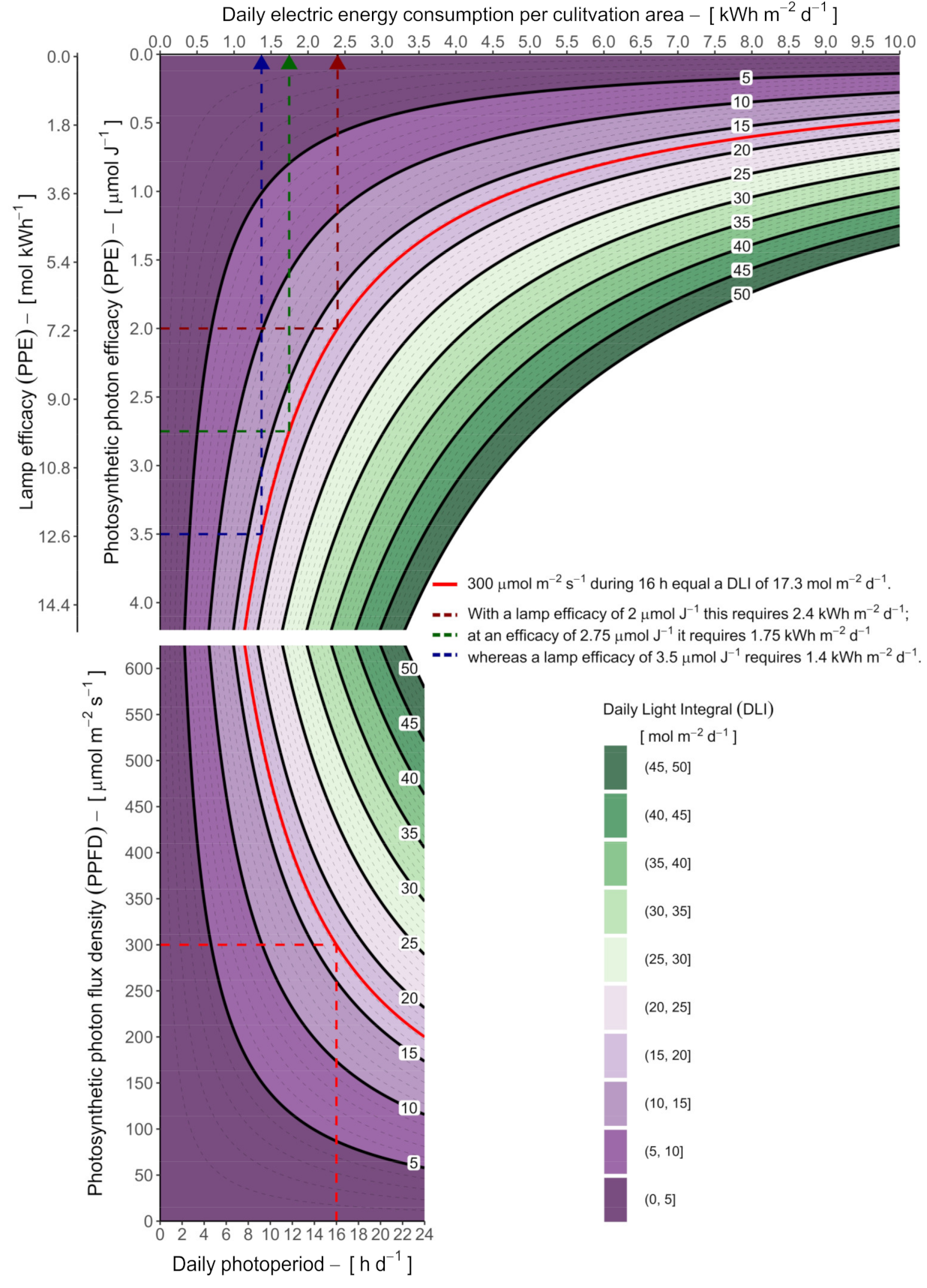
2.5.2. Indoor Cultivation in Growth Room with Sole-Source Lighting

The indoor growth room cultivation phase under sole-source lighting was assumed to be of 92 days, from 1 November to 31 January using a photoperiod of 16 h·d−1 at a constant PPFDlamps of 300 µmol·m−2·s−1. These conditions are similar to those that have already been tested in different studies in the region [18,25,82,90,119,120]. Using Equation (4), the resulting DLIlamps is 17.3 mol·m−2·d−1 which is considered enough for most cut flowers, greenhouse vegetables, and forest seedlings [8,9,28,31]. The lamps were assumed to be adjustable LED fixtures with efficacies equal to either:
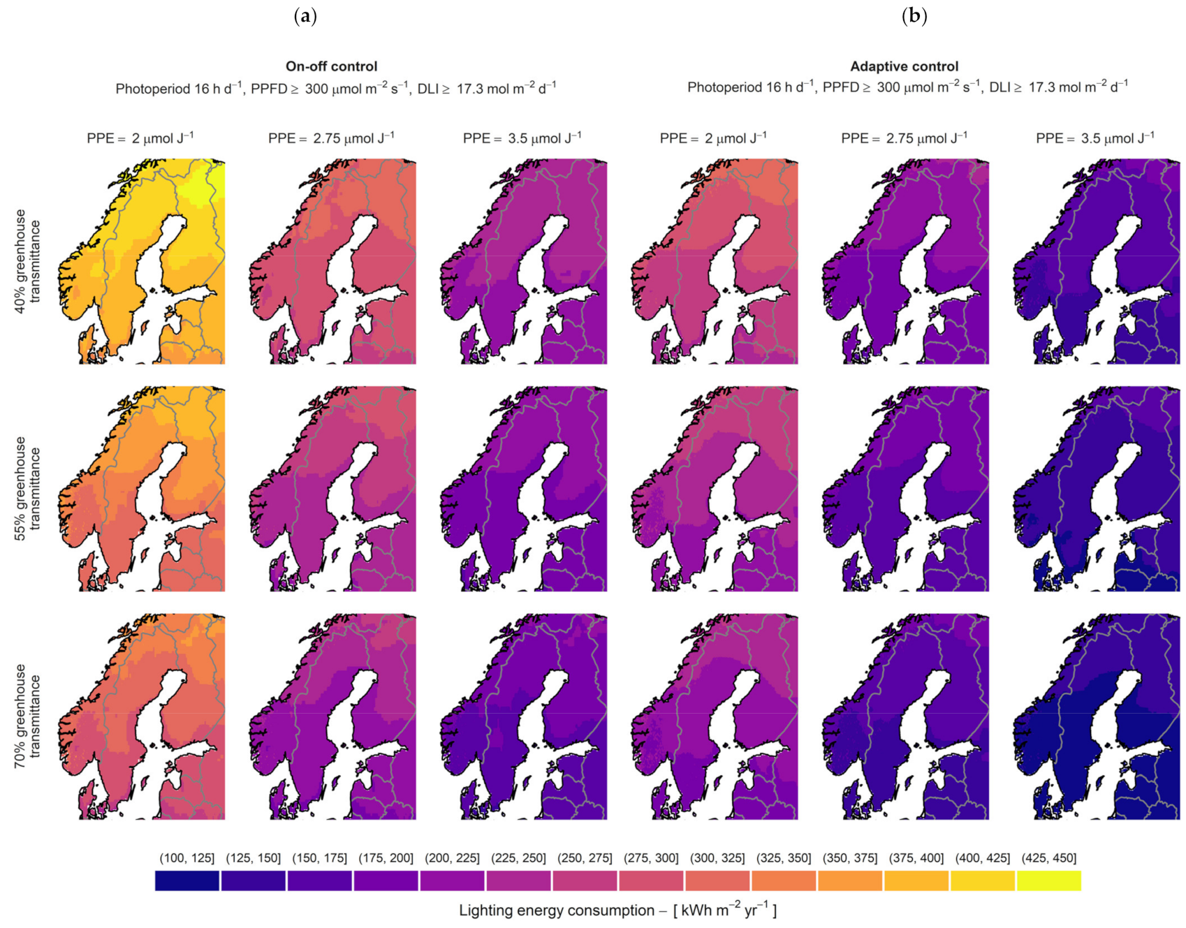
  • PPE = 2.0 µmol·J−1, considering a standard LED luminaire;
  • PPE = 2.75 µmol·J−1, for a state-of-the-art standard, LED luminaire;
  • PPE = 3.5 µmol·J−1, to account for upcoming developments.

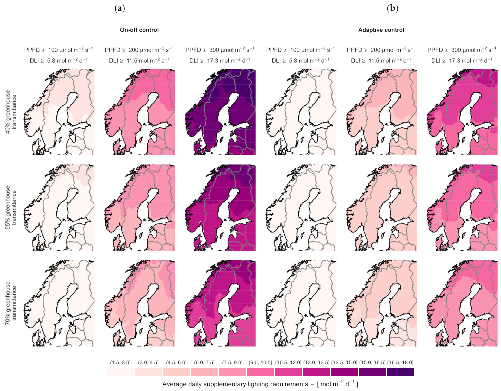
2.5.3. Greenhouse Cultivation with Supplementary Lighting

The assumed greenhouse cultivation period consisted of 181 days, from 1 February to 20 May and from 20 August to 31 October. The objective was to maintain at least the set PPFDthreshold (100, 200, or 300 µmol·m−2·s−1) inside the greenhouse during a 16 h·d−1 photoperiod (04:00–20:00) to reach the minimum equivalent DLIthreshold value.
The hourly average natural light levels inside the greenhouse (PPFDgreenhouse) were calculated using Equation (7) for the different values of τh, PAR (40%, 55%, or 70%). Then, the two lighting control protocols were compared using Equations (8) and (9) to calculate the hourly supplementary light provided by the lamps (PPFDlamps). The average daily supplementary lighting requirement (DLIlamps) was determined by adding the hourly PPFDlamps values using Equation (3) and dividing it by the number of cultivation days.
The same three PPE values as in the sole-source lighting phase were assumed. The energy consumption corresponding to the DLIlamps was estimated using Equation (5) for the different PPFDthreshold settings and added for the complete season at each location in the geographic grid. Table 1 shows a summary of the parameters used for the calculations during the greenhouse cultivation period.

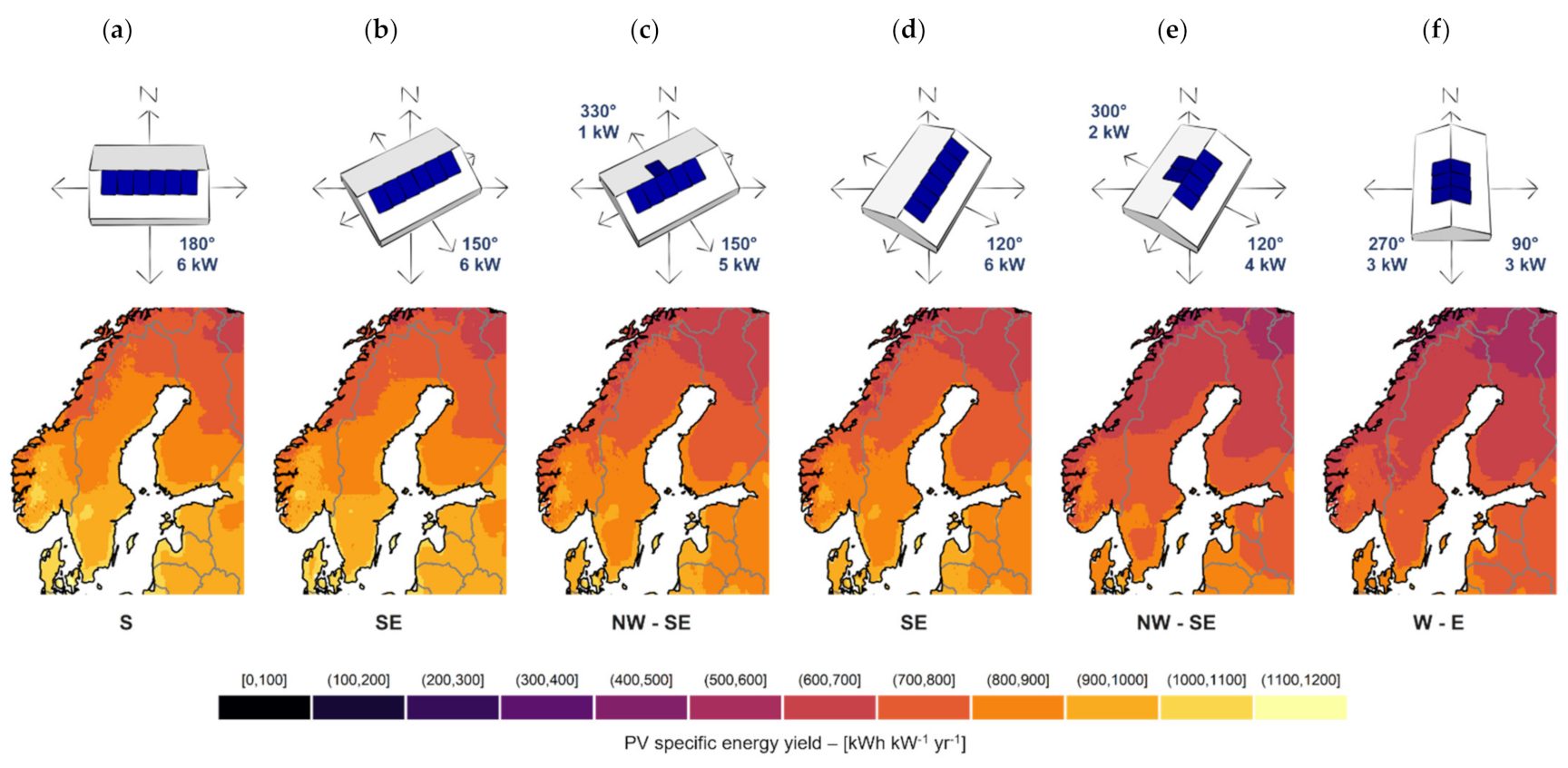
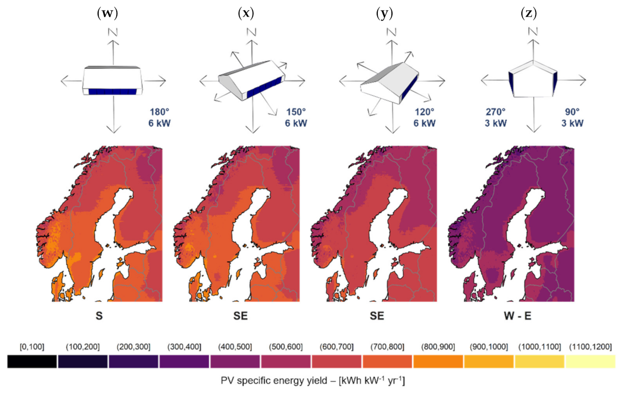
2.6. Photovoltaics on Greenhouses

The nominal peak power of a PV installation (PPV, STC, W) is a quantity used in industry to describe the output measured at standard test conditions (STC). The STC are defined for the device temperature (TPV = 25 °C), input irradiance (GSTC = 1000 W·m−2), and light spectrum (Air mass 1.5) [121]. The efficiency at STC (ηSTC, %) relates the PPV, STC to the input irradiance (GSTC) over the PV area (APV, m2) as shown in Equation (10).
Commercially available PV modules have efficiencies ranging from 12–22% depending on their material [122]. Different PV technologies have differences in their spectral responsivity and thermal behaviors. In practice, however, it is usually assumed that systems with equal PPV,STC will have a similar yearly energy output [123]. When the ηSTC is known, Equation (10) can be used to calculate the surface needed for a specific PPV,nom.
η STC , % = P PV ,   STC G STC · A PV · 100
The ratio between the APV and the available area on the ground or roof (Aground or Aroof, m2) is called the PV coverage ratio (PVR) (Equation (11)). Selecting the ideal PVR value is an optimization task that should balance the electricity output goals with the light requirements of the species to cultivate, also considering the irradiance available at the location and the transmittance of the greenhouse [59,64,65,70].
PV R , % = A PV A roof · 100
Once the target PVR is decided either by calculations or measurements, Equation (12) can be used to estimate the maximum recommended PPV,STC that should be installed as a function of the efficiency of the PV modules and the roof area of the greenhouse.
P PV , STC PV R · A roof G STC · η STC
Neither a specific PPV,STC or PVR were defined for this study; instead, relative energy output values were estimated which can then be used later to choose the system size.

PV System Parameters

The energy output of a PV system depends on many aspects besides the installed peak power and the irradiance at the location. Among the main factors influencing the yield are the temperature, the tilt and orientation of the surface (also known as slope and azimuth angle), and the material of the solar cells [123]. Considering these parameters [71], PVGIS was used to estimate the monthly energy output of different PV system configurations in multiple locations. The same geographic grid and data source (ECMWF-ERA-5) were used as previously described.
The PV modules were assumed to be mounted either on the roof with a slope of 25° or the wall (slope of 90°) of a wide-span greenhouse with a double-pitched roof, typical of northern Europe [116,124]. A symmetrical yearly irradiance around the North-South line was assumed; implying that an inclined surface with an azimuth towards the East receives the same amount of sunshine as one with the same angle mirrored towards the West. Four different orientations were compared using the direction perpendicular to the roof ridge as reference. The corresponding azimuth angle was measured clockwise using the navigation convention with North = 0° [93]. For some of the orientations, the planned PPV,STC was divided between two surfaces in opposing directions (see Table 2).
The following system parameters were used in common for all systems and locations; a detailed explanation of the parameters can be found in the user manual of PVGIS [70]:
  • PPV,STC: 6 kW;
  • PV technology: crystalline silicon (c-Si);
  • mounting position: fixed and building-integrated;
  • horizon: yes;
  • estimated system losses: 14% (PVGIS default).
A system size of 6 kW was chosen for all the configurations because this amount allows to easily divide the planned PPV,STC among the two sides of the roof using whole number ratios (6:0, 5:1, 4:2, 3:3) that can be later scaled to larger systems. Finally, the yearly energy output (EPV, kWh·yr−1) extracted from PVGIS was divided by the PPV,STC to obtain the PV specific energy yield (Erel,PV, kWh·kW−1·yr−1) for all locations.

2.7. Data Analysis

The analysis of the different parameters was performed using the statistical software R version 4.1.1 [125] with the tidyverse package collection for the various calculations [126,127] including the division in bins and interpolations for the contour plots. The vector data for the maps were plotted using ggplot2 [128,129] and sf packages [130,131]. The geographical data of the different regions were retrieved from the public dataset Natural Earth [132] using the R package rnaturalearth [133].

3. Results

3.1. Outdoor Ambient Conditions

The environmental data extracted confirmed the strong seasonal variations in the north European region. The monthly average daily ambient temperature (Figure 1 and Figure A1 for Iceland) ranged during the winter between −20 °C and −15 °C in the northern and mountainous areas. For most of the regions, the temperature remained below 0 °C for several months. Only in Denmark and the southernmost part of Sweden, the monthly average temperature stays above freezing for the complete year. In contrast, the summer months exhibited average temperatures close to 20 °C for the Baltic countries, Denmark, and half of Sweden and Finland. Norway and Iceland had lower summer temperatures averaging closer to 15 °C. The coldest temperatures were registered during January and February while the warmest period was in July and August. Since these are averaged values, the actual temperatures are expected to reach beyond these levels, accounting for differences of more than 60 °C between summer and winter.
The available light also varied drastically between the seasons and along the different latitudes analyzed; changing the duration of the photoperiod (Figure 2) as well as the daily amount of light suitable for photosynthesis (Figure 3 and Figure A2). The daylength in the south (latitude 55° N) changed from 6.5 h in the winter to almost 18 h in summer. In the northernmost latitudes, the day length shifted between days of constant sunshine in summer to periods in the winter when the sun remained below the horizon.
The DLI levels (Figure 3 and Figure A2) also exhibited a large variation, reaching a maximum range of 45–50 mol·m−2·d−1 during summer; contrasting to the minimum range in winter between 0–5 mol·m−2·d−1. Figure 4 and Figure A3 show how the proportion of scattered light (Gd/Gh) increases after the summer months, being more than 40% from August to March in most locations. Although the climate is a very complex system with many factors intertwined, the regions with lower ratios of diffuse light (which is related to the cloudiness) match well to the regions with higher DLI and warmer summers.

3.2. Sole-Source Lighting Requirements

The DLI maps and the photoperiod lengths (Figure 2, Figure 3 and Figure A2) can be used as a reference for the light levels required during indoor cultivation. The chosen photoperiod of 16 h·d−1 roughly corresponds to the daylengths during early spring (March–April) or early autumn (late August–September) depending on the latitude. Setting the intensity of the lamps to PPFDlamps = 300 µmol·m−2·s−1 during the entire photoperiod creates a DLIlamps of 17.3 mol·m2·d1 which also matches well the outdoor DLIsun levels during those seasons.
Having these settings and the resulting DLIlamps, Figure 5 combines Equations (3)–(6) to calculate the daily electric energy consumption for the cultivation area based on the efficacy of the lamps. A standard LED fixture with a PPE = 2 µmol·J−1 would require daily 2.4 kWh·m−2 while a state-of-the-art luminaire with PPE = 2.75 µmol·J−1 could reduce the energy consumption by 27% to 1.75 kWh·m−2·d−1. Expected technological improvements in LEDs (PPE ≈ 3.5 µmol·J−1) could bring the savings further down for consumption of 1.4 kWh·m−2·d−1 under the same settings. During the assumed 92 days of indoor cultivation with sole-source lighting, the growth room would require 221 kWh·m−2, 161 kWh·m−2, or 129 kWh·m−2 of electricity for lighting considering these respective lamp efficacies.

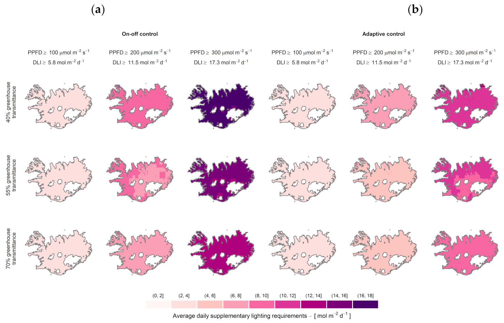
3.3. Greenhouse Supplementary Lighting Requirements

The parametric analysis of the greenhouse supplementary lighting showed a large variation across the different settings. When comparing only the control protocols for all locations while maintaining the other variables equal, the average supplementary light delivered was always lower for the adaptive control (Figure 6 and Figure A4 for Iceland; panels a vs. b). The differences ranged between 0.3 and 1.5 mol·m−2·d−1 for the lowest PPFDthreshold of 100 µmol·m−2·s−1, from 1.1 to 3.6 mol·m−2·d−1 at 200 µmol·m−2·s−1, and for 300 µmol·m−2·s−1 the difference range went from 2.4 to 5.7 mol·m−2·d−1.
At the lowest PPFDthreshold of 100 µmol·m−2·s−1, regardless of the control protocol, the light transmitted into the greenhouse was often enough to reach the threshold resulting in a lower need for supplementary light. Only when the transmittance was below 55% combined with the on-off control protocol did the supplementary lighting requirements increase to 4.5 mol·m2·d1 in some places (see Figure 6, upper left corner). The transmission levels caused larger differences when using the on-off protocol (observed when comparing by rows in Figure 6 and Figure A4). The reason is that with the on-off protocol the lamps are assumed to be turned on at full power when the threshold is not reached; with lower transmittance and higher thresholds settings, this happens more often.
As the PPFDthreshold increased, these combined effects were more evident. In the “worst-case scenario”, with the lowest transmittance and the highest PPFDthreshold, the differences between control protocols were higher (Figure 6 and Figure A4, upper right corner in each panel). In this setting, the available natural light inside the greenhouse did not reach the minimum threshold during most of the day. While the adaptive control was able to make use of the low available light and provide only the difference to reach the threshold; with the on-off protocol, the lamps were active at full power throughout the entire photoperiod (DLIthreshold = DLIlamps).
The electrical energy needed for lighting was calculated considering the three different lamp efficacies. Figure 7 and Figure A5 show the estimated yearly consumption during the 181 days of greenhouse cultivation using the highest PPFDthreshold of 300 µmol·m−2·s−1.
The variations in the Eel, lamps follow similar trends as the supplementary light requirements regarding greenhouse transmittance and lighting control protocols. However, the differences were more pronounced between the PPFDthreshold levels due to the interaction effects with the PPE of the lamps, where lower efficacy values resulted in higher energy consumptions (comparing by column in Figure 7 and Figure A5).
The energy consumption approaches infinity as the PPE decreases (Figure 5). This means that at some point the DLIthreshold can become too high and it is not possible for lamps with very low efficacy to supply it. When the PPFDthreshold was set to 100 µmol·m−2·s−1, the maximum Eel, lamps range was 110–120 kWh·m−2·yr−1; doubling the value raised the highest range to 280–300 kWh·m−2·yr−1 (data not shown). Finally, the PPFDthreshold of 300 µmol·m−2·s−1 (Figure 7 and A5) resulted in a maximum range of 425–450 kWh·m−2·yr−1.

3.4. PV Systems Specific Energy Yield

The specific energy yield of the roof-mounted PV systems varied between the different regions and system designs, ranging from around 400 to 1120 kWh·kW−1·yr−1. This almost threefold increase is clearly shown in Figure 8 (data for Iceland not shown); where the output decreases noticeably as the latitude increases. The output also gradually decreases as the azimuth turns away from the optimal south-facing orientation (Figure 8a) towards an east-west layout (Figure 8f). Shifting some of the installed power from the south-east-facing roof onto the north-west roof side reduced the relative output (Figure 8, panel b vs. c and panel d vs. e). The coastal regions, particularly along the Baltic Sea presented higher PV outputs compared to areas inland at the same latitude.
The yearly specific yields of wall-mounted PV systems also presented a wide variation from around 400 to 925 kWh·kW−1·yr−1 for the same installed power (Figure 9). However, with vertically mounted PV modules, the effect of the latitude became less important when the azimuth rotated away from 180° facing south. Systems distributed at a combined azimuth of 90° and 270° towards the east-west (Figure 9z), had a much lower variation along the latitude with all the locations presenting specific system yields in the range of 400–600 kWh·kW−1·yr−1. Interestingly, PV modules on the south and south-east facade (azimuths 180° and 150°; in Figure 9w,x), presented similar specific energy yield as the combined roof-mounted systems with azimuths 120° and 300° (Figure 8e) and azimuths 90° and 270° (Figure 8f) respectively.

3.5. Year-Round Concept Implementation for One Location

Perhaps the best way to describe the year-round cultivation concept is to calculate the values for one location. Table 3 shows the average monthly values for the environmental variables extracted for the city of Borlänge, Sweden (lat. 60.5° N, lon. 15.4° E); showing the different cultivation phases as well. The day length can be found in Figure 2.
Using the following parameters for indoor cultivation at PPFDlamps = 300 µmol·m−2·s−1 during a photoperiod of 16 h·d−1 would result in a DLIlamps of 17.3 mol·m 2·d 1. These settings agree well with the average DLIsun values for March and October in this location (Table 3). Depending on the efficacy of the lamps (using Figure 5b), 92 days of indoor cultivation would require 221 kWh·m−2, 161 kWh·m−2, or 129 kWh·m−2.
Table 4 presents the estimated daily supplementary lighting requirements and corresponding electric energy consumption for lighting during the greenhouse cultivation phase (181 days), according to the different parameter values for the two control protocols.
Assuming a moderate greenhouse transmittance of 55% and using an on-off control protocol, the lamps would provide on average 12.9 mol·m−2·d−1 of supplementary lighting. Depending on the efficacy, the corresponding energy consumption for the whole greenhouse cultivation period of 181 days would be 325 kWh·m−2yr−1 for standard LED lamps, 236 kWh·m−2yr−1 if state-of-the-art standard LED luminaires are used and future developments could potentially reduce it to 185 kWh·m−2yr−1 (see Table 4, orange shades).
For comparison, the adaptive control protocol (Table 4, purple shades) would provide instead 9.0 mol·m−2·d−1 of supplementary lighting. Which, depending on the efficacy of the lamps, would translate into 227 kWh·m−2yr−1, 165 kWh·m−2yr−1 or 130 kWh·m−2yr−1 for the same period. Finally, selecting state-of-the-art standard LED luminaires for both indoor and greenhouse cultivation as well as adaptive control would require per year an estimate of 326 kWh·m−2yr−1 (161 kWh·m−2 for 92 days of indoor cultivation and 165 kWh·m−2 for 181 days of greenhouse cultivation).
Knowing the energy requirements makes it possible to estimate the needed PPVSTC and as well as how many m2 of cultivation with supplementary lighting can be compensated with the installed PV. The yearly specific energy yields for the different greenhouse integrated PV systems at this location are shown in Table 5. The different system types correspond to those presented in Table 2 and Figure 8 and Figure 9.
In a commercial greenhouse (assuming a roof area, Aroof = 2000 m2) cultivating of a shade-intolerant species that would be negatively affected if PVR,% ≥ 15%; the maximum PPV,STC installed could be 54 kW with PV modules of 18% efficiency (using Equation (12)). If all PV modules are installed on a south-facing roof (Table 5, system a), the expected yearly electrical yield would be 48,816 kWh·yr−1. Considering an example of a forest nursery producing Scots pine (Pinus sylvestris L.) seedlings on a year-round basis using an LED growth room during germination and early growth [18,25,86,134], the electricity generated by the PV of the greenhouse would be enough to compensate for the lighting of roughly 300 m2 of indoor cultivation for 92 days during the winter months.

4. Discussion

Although in optimal conditions, many species could grow better and produce higher quality plants when growing outdoors due to the higher light levels, better air movement, lower relative humidity, and less overheating [28,31]; damages to the crops due to climate phenomena such as droughts and floods as well as biological menaces such as pests and diseases considerably affect and reduce productivity. For species that can be cultivated entirely in greenhouses, this option presents a more sustainable and resource-efficient form of cultivation [6,10].
In the Nordic countries, the outdoor vegetation period is very short and limited to only a few months, restricting the outdoor cultivation of crops like herbaceous perennials, forest seedlings, and other potted plants that are grown for more than one season. During the summer, there are long days with abundant sunlight, the DLIsun levels peak in June, and the warmest temperatures come in July and August (Figure 1, Figure 2 and Figure 3). In contrast, during the winter the available PAR light is almost negligible, and the temperatures can go well below the freezing point during several weeks in most parts of the region.
The year-round cultivation concept presented here aims to work with the harsh northern climate and adapt to the natural conditions instead of trying to go against them. When the outside environment is not suitable anymore for cultivation, the plants can be transported inside modern greenhouses with transparent covers which present the best option to provide additional heating and supplementary lighting to the plants [10,110].
The amount of natural light reaching inside a greenhouse depends heavily on multiple factors including the building design [114,124], roof shape and inclination [110,115], location and orientation [135], the position of the supporting structures as well as hanging objects inside like pots or lamps [111,136], and the covering material of the greenhouse [116,117,137,138]. Weathering and aging of the glazing as well as other local factors like condensation, dust, snow accumulation, and buildings nearby can obstruct the light that enters a greenhouse [112].
From all these factors, the covering material is probably one of the most important for light transmission and therefore has been broadly studied [110]. Distinct wavelengths behave differently depending on the material composition and the angle of incidence, affecting the spectral distribution at the cultivation area [137,139]. Determining the natural light inside a greenhouse involves complex calculations once the main specifications such as location, structure design, and covering material have been decided [4,64,113,140]; or requires extensive simultaneous measurements of the outdoors and indoors illumination levels [110,111,116,117]. Instead, the parametric study here described aimed to provide a broad perspective and a range of plausible hemispherical PAR transmittance values within reasonable limits ranging from 40% to 70%.
Compared to other environmental variables, the amount of PAR inside modern greenhouses is usually less accurately regulated and depends heavily on outdoor conditions [9,112]. Different greenhouse lighting control protocols have been proposed in the past including strategies for extending the day length [9,10,141], ensuring a consistent DLI [39], and using adaptive control to reach a minimum PPFD threshold [40,42]. Usually, the implementation of these concepts has been restricted to the technical limitations of the available HID lamps. However, as LED grow lights become commonly adopted, more advanced and dynamic control protocols can benefit from the LEDs flexible spectra, dimmability, rapid response, and tolerance to numerous switching cycles [142].
Two supplementary lighting control protocols were compared in this study: on-off and adaptive control. Regardless of parameter combinations and locations, the adaptive LED lighting control had the best outcomes with the lowest supplementary lighting requirements. The adaptive control allowed to reach and maintain the PPFDthreshold throughout the entire photoperiod while considering the natural light inside the greenhouse. This resulted in lower energy consumption for lighting. The potential energy savings that followed could justify doing a lamp retrofit in relatively new greenhouses that are in good conditions but still use HID lamps [7,51,54].
Although greenhouses can extend the cultivation period during spring and autumn in the Nordics, at some moment in the year, there is very low radiation gain from the sun and too high heat loss through the glazing. In the summer, the opposite happens as it becomes difficult to naturally dissipate the excess heat from the abundant sunlight [4,116].
Closed plant production systems with sole-source lighting are designed to maximize the yield using multi-level cultivation and have the advantage of a standardized and controlled environment independent from outdoor conditions. Nevertheless, they also have the evident disadvantage of excluding sunlight which is a valuable and free resource. This results in the high energy consumption for lighting and climate control [55,112]. It has been estimated that between 70% and 80% of the electricity consumption in indoor growth rooms is due to lighting while the rest is mainly cooling and dehumidification [53,142].
Increasing the planting density assures a better use of the space and selecting efficient lamps prevents unnecessary energy consumption. The efficacy of growth lights has developed significantly in the past years, especially for LEDs. In 2014 the best-in-class HID and LED lamps had similar efficacies of around 1.70 µmol·J−1 [7,143]. While HID lamps were improved to 2.1 µmol·J−1 by 2018 [7,144,145]; LED fixtures in 2020 reached efficacies between 2.5 and 2.8 µmol·J−1 and are expected to reach even higher values between 3.4 and 4.1 µmol·J−1 during this decade [54]. Irrespectively of how advanced the lighting technologies are, there will always exist a certain investment and energy cost for artificial lighting compared to sunlight [51]. Under some circumstances and for certain species, the advantages of a fully controlled growth space and the possibility of year-round cultivation might outweigh some of those costs [52,53,55].
To partly offset the energy used for supplementary lighting during the darker months, some of the solar energy abundant during the summer can be transformed into electricity integrating PV on the roof of the greenhouses. Agrivoltaics can reduce the competition for space between energy and plants production but if not planned carefully it can increase competition for sunlight [57]. Hence, proper optimization for the particular location and targeted plant species is required, depending on if the main goal is to maximize crop yield or increase the electrical output [58,59].
Using Equation (10), it was possible to calculate that 1 kW of PV with 18% efficiency takes up approximately 5.6 m2 and if it is mounted on a south-facing roof of a greenhouse or growth chamber (Table 5, system a), each m2 of PV will have a yearly output of 162.5 kWh·m−2·yr−1. This corresponds more or less with the amount of electricity for lighting needed per m2 in a location in mid-Sweden, either for indoor cultivation for 92 days or greenhouse cultivation for 181 days. Nevertheless, concluding that 1 m2 of PV would compensate the lighting for 1 m2 of cultivation would not be correct. The scenarios presented in this study assumed only 92 days of indoor cultivation with sole-source lighting, however, one of the main purposes of a growth room is to save space by using multi-layer cultivation on a year-round basis. This means that the growth area and cultivation time indoors would be by several factors larger for the available roof area directly on the growth room [52,55].
An adequate PVR requires considering the shading effect that the integrated PV will have inside the greenhouse and its impact on the light levels for the crop. Plant species with a low (5–10 mol·m−2·d−1) and moderate light needs (10–20 mol·m−2·d−1) are more tolerant to shading compared to plants with high (20–30 mol·m−2·d−1) or very high (DLI > 30 mol·m−2·d−1) requirements [28,29,30,31,32]. Greenhouses in southern Europe with a PVR,% between 10% and 15% showed a very small decrease in the crop yields, even when cultivating shade-intolerant plants like tomatoes [66,69]. Roof coverage ratios between 20–25% showed minimal negative effects on the yield of low and moderate light-demanding species [59,70]. However, at higher coverage ratios (PVR,% ≥ 60%) even species requiring moderate light were affected [70].
Naturally, parametric studies like the one here presented come with clear limitations due to the great number of variables assumed. For the implementation of greenhouses with integrated PV in the Nordics, additional studies with detailed simulations for specific locations are necessary to determine the ideal PV coverage ratios for different species when cultivated in the region and how the greenhouse environment can influence the PV energy yield. Practical implementation of the concept will increase the understanding and validate the results while providing valuable data for the improvement of the concept.
Finally, the electrical equipment used inside the growth rooms and greenhouses will have an important effect on the ambient temperature in the cultivation area. The lamps’ efficiency, as well as the amount of time they are used, can impact the amount of heating and cooling load necessary. Although not included in the scope of this study, these types of calculations are necessary for the year-round cultivation concept using LED lamps and some examples regarding the thermal energy requirements for controlled-environment cultivation exist already in the literature [4,55,146,147,148].

5. Conclusions

New technological developments such as LED grow lights, adaptive lighting control protocols, as well as greenhouse integrated PV, have the potential of making the concept of year-round cultivation a feasible option, even in the harsh conditions of the Nordic countries. After analyzing satellite meteorological data for the region, it can be concluded that:
  • Ambient temperature and natural DLI levels are suitable for outdoor cultivation during at least three months in the summer for most of the region.
  • Greenhouses can be used to start the cultivation earlier in spring and extend the vegetation period until later in autumn.
  • Transmittance levels of natural light inside the greenhouse can significantly influence the supplementary lighting needed for the plants.
  • Among the options compared, LED lamps with adaptive lighting control have the highest energy-saving potential. They can benefit from the available sunlight inside the greenhouse, avoiding unnecessary energy waste and supplementing only enough light to reach the DLI target for the cultivated species.
  • During the winter months, indoor cultivation in closed growth chambers offers a standardized and controlled environment independent from outdoor conditions.
  • Light intensity and duration of the photoperiod together with the efficacy of the lamps determine the amount of electricity needed for lighting in the growth room.
  • Greenhouses with integrated PV provide an alternative for using the abundant sunshine in the summer and offsetting some of the electricity used for lighting during the darker months.
  • To avoid negative effects on the plants caused by excessive shading from the solar panels, careful planning is required based on the design, location, and orientation of the greenhouse.
  • Additional studies that consider the investment and running costs for heating and cooling of the growth rooms and greenhouses with regard to the lighting control protocols and LED lamps are necessary. Only when both electrical and thermal energy requirements are evaluated together can the feasibility of the year-round cultivation concept be truly evaluated.

Funding

This research project was supported by FP7 Environment [Grant Number ZEPHYR-Project ID: 308313].

Data Availability Statement

Publicly available datasets were analyzed in this study. This data can be found here: PVGIS © European Communities, 2001–2021.

Acknowledgments

The author would like to thank Anders Mattsson (Dalarna University), Frank Fiedler (Dalarna University), Uwe Zimmermann (Uppsala University), and Sofia Lindblad (Uppsala University) for their constructive comments on the content and general improvements. The irradiance and meteorological data as well as the PV simulations were extracted from PVGIS © European Communities, 2001–2021.

Conflicts of Interest

The authors declare no conflict of interest. The funders had no role in the design of the study; in the collection, analyses, or interpretation of data; in the writing of the manuscript, or in the decision to publish the results.

Appendix A

The figures presented in this appendix are similar to those in the main text but for the region covering Iceland. The data was retrieved from the same source, from 63° N to 67.5° N in latitude and from 13° E to 25° E in longitude using a cell size of 0.05° × 0.05° in both latitude and longitude.
Figure A1. Monthly average daily ambient temperature maps for Iceland. Values from the ECMWF-ERA-5 dataset with a coverage period of 2005–2016 retrieved from PVGIS as a 0.05° × 0.05° grid both in latitude and longitude, extending from 63° N to 67.5° N in latitude and 13° W to 25° W in longitude.
Agriculture 11 01255 g0a1
Figure A2. Monthly average photosynthetic daily light integral (DLIsun, mol·m−2·d−1) maps for Iceland. Values from the ECMWF-ERA-5 dataset with a coverage period of 2005–2016 retrieved from PVGIS as a 0.05° × 0.05° grid both in latitude and longitude, extending from 63° N to 67.5° N in latitude and 13° W to 25° W in longitude.
Agriculture 11 01255 g0a2
Figure A3. Monthly average diffuse fraction of global horizontal irradiance (Gd/Gh) for Iceland. Values from the ECMWF-ERA-5 dataset with a coverage period of 2005–2016 retrieved from PVGIS as a 0.05° × 0.05° grid both in latitude and longitude, extending from 63° N to 67.5° N in latitude and 13° W to 25° W in longitude.
Agriculture 11 01255 g0a3
Figure A4. Average daily supplementary lighting requirements (DLIlamps, mol·m−2·d−1) maps of Iceland for the chosen greenhouse cultivation period of 181 days: from 1 February to 20 May and from 20 August to 31 October. A photoperiod of 16 h·d−1 was assessed considering three minimum light settings (PPFDthreshold: 100, 200 or 300 µmol·m−2·s−1) and three possible greenhouse hemispherical transmittances (τh, PAR: 40%, 55% or 70%). The two panels compare different control protocols: (a) On-off control vs. (b) Adaptive control. Values presented as a 0.05° × 0.05° grid both in latitude and longitude, extending from 63° N to 67.5° N in latitude and 13° W to 25° W in longitude.
Agriculture 11 01255 g0a4
Figure A5. Yearly lighting energy consumption (Eel, lamps, kWh·m−2·yr−1) maps of Iceland for the chosen greenhouse cultivation period of 181 days: from 1 February to 20 May and from 20 August to 31 October. The electric energy demand of the lamps was calculated for a photoperiod of 16 h·d−1 with a PPFDthreshold of 300 µmol·m−2·s−1, considering three different photosynthetic photon efficacies (PPE: 2, 2.75 or 3.5 µmol·J−1) and three possible greenhouse hemispherical transmittances (τh, PAR: 40%, 55% or 70%). The two panels compare different lighting control protocols: (a) On-off control; (b) Adaptive control. Values presented as a 0.05° × 0.05° grid both in latitude and longitude, extending from 63° N to 67.5° N in latitude and 13° W to 25° W in longitude.
Agriculture 11 01255 g0a5

References

  1. Swedish Meteorological and Hydrological Institute (SMHI) Climate Indicators—Length of Vegetation Period. Available online: https://www.smhi.se/en/climate/climate-indicators/climate-indicators-length-of-vegetation-period-1.91482 (accessed on 23 August 2020).
  2. Albright, L.D.; Langhans, R.W. Controlled Environment Agriculture Scoping Study; Electric Power Research Institute: Ithaca, NY, USA, 1996. [Google Scholar]
  3. Despommier, D. The Vertical Farm: Feeding the World in the 21st Century; Macmillan: New York, NY, USA, 2010. [Google Scholar]
  4. Vadiee, A.; Martin, V. Energy Analysis and Thermoeconomic Assessment of the Closed Greenhouse—The Largest Commercial Solar Building. Appl. Energy 2013, 102, 1256–1266. [Google Scholar] [CrossRef]
  5. Nimmermark, S.; Nielsen, J.M. Klimatisering, Belysning, Bevattning Och Mekanisering I Växthus; Alnarp, Sweden, 2014; p. 30. [Google Scholar]
  6. Stanghellini, C.; Van’t Ooster, B.; Heuvelink, E. Greenhouses: Why? In Greenhouse Horticulture; Wageningen Academic Publishers: Wageningen, The Netherlands, 2018; pp. 15–25. ISBN 978-90-8686-329-7. [Google Scholar]
  7. Nelson, J.A.; Bugbee, B. Economic Analysis of Greenhouse Lighting: Light Emitting Diodes vs. High Intensity Discharge Fixtures. PLoS ONE 2014, 9, e99010. [Google Scholar] [CrossRef] [PubMed] [Green Version]
  8. Fisher, P.; Both, A.J.; Bugbee, B. Supplemental Lighting—Technology, Costs, and Efficiency. In Light Management in Controlled Environments; Lopez, R., Runkle, E.S., Eds.; CreateSpace Independent Publishing Platform: Willoughby, OH, USA, 2017; pp. 74–81. ISBN 978-1-5442-5449-4. [Google Scholar]
  9. Landis, T.D.; Tinus, R.W.; McDonald, S.E.; Barnett, J.P. Chapter 3: Light. In Atmospheric Environment—The Container Tree Nursery Manual; Agriculture Handbook 674; USDA Forest Service: Washington, DC, USA, 1992; Volume 3, p. 145. [Google Scholar]
  10. Nelson, P. Greenhouse Operation and Management, 7th ed.; Pearson: Boston, MA, USA, 2011; ISBN 978-0-13-243936-7. [Google Scholar]
  11. Runkle, E. Strategies for Supplemental Lighting; Greenhouse Product News: Sparta, MI, USA, 2009; p. 50. [Google Scholar]
  12. Bugbee, B. Effects of Radiation Quality, Intensity, and Duration on Photosynthesis and Growth; Plants, Soils, and Biometeorology Department Utah State University: Logan, UT, USA, 1994; N96-18128; p. 12. [Google Scholar]
  13. Aphalo, P.J.; Ballaré, C.L.; Scopel, A.L. Plant-Plant Signalling, the Shade-Avoidance Response and Competition. J. Exp. Bot. 1999, 50, 1629–1634. [Google Scholar] [CrossRef]
  14. Aphalo, P.J. Light Signals and the Growth and Development of Plants—A Gentle Introduction; Department of Biosciences Plant Biology University of Helsinki: Helsinki, Finland, 2010. [Google Scholar]
  15. McCree, K.J. The Action Spectrum, Absorptance and Quantum Yield of Photosynthesis in Crop Plants. Agric. Meteorol. 1971, 9, 191–216. [Google Scholar] [CrossRef]
  16. McCree, K.J. Test of Current Definitions of Photosynthetically Active Radiation against Leaf Photosynthesis Data. Agric. Meteorol. 1972, 10, 443–453. [Google Scholar] [CrossRef]
  17. Craver, J.K.; Lopez, R.G. Control of Morphology by Manipulating Light Quality and Daily Light Integral Using LEDs. In LED Lighting for Urban Agriculture; Springer: Berlin/Heidelberg, Germany, 2016; pp. 203–217. [Google Scholar]
  18. Riikonen, J.; Kettunen, N.; Gritsevich, M.; Hakala, T.; Särkkä, L.; Tahvonen, R. Growth and Development of Norway Spruce and Scots Pine Seedlings under Different Light Spectra. Environ. Exp. Bot. 2016, 121, 112–120. [Google Scholar] [CrossRef]
  19. Bantis, F.; Radoglou, K. Morphology, Development, and Transplant Potential of Prunus avium and Cornus sanguinea Seedlings Growing under Different LED Lights. Turk. J. Biol. 2017, 41, 314–321. [Google Scholar] [CrossRef]
  20. Hernandez, R.; Kubota, C. Light Quality and Photomorphogenensis. In Light Management in Controlled Environments; Lopez, R., Runkle, E.S., Eds.; CreateSpace Independent Publishing Platform: Willoughby, OH, USA, 2017; pp. 29–37. ISBN 978-1-5442-5449-4. [Google Scholar]
  21. Stuefer, J.F.; Huber, H. Differential Effects of Light Quantity and Spectral Light Quality on Growth, Morphology and Development of Two Stoloniferous Potentilla Species. Oecologia 1998, 117, 1–8. [Google Scholar] [CrossRef] [PubMed]
  22. Marcelis, L.F.M.; Broekhuijsen, A.G.M.; Meinen, E.; Nijs, E.; Raaphorst, M.G.M. Quantification of the Growth Response to Light Quantity of Greenhouse Grown Crops. In Proceedings of the V International Symposium on Artificial Lighting in Horticulture 711, Lillehammer, Norway, 21–24 June 2005; pp. 97–104. [Google Scholar]
  23. Gerovac, J.R.; Craver, J.K.; Boldt, J.K.; Lopez, R.G. Light Intensity and Quality from Sole-Source Light-Emitting Diodes Impact Growth, Morphology, and Nutrient Content of Brassica Microgreens. HortScience 2016, 51, 497–503. [Google Scholar] [CrossRef] [Green Version]
  24. Poorter, H.; Niinemets, Ü.; Ntagkas, N.; Siebenkäs, A.; Mäenpää, M.; Matsubara, S.; Pons, T. A Meta-Analysis of Plant Responses to Light Intensity for 70 Traits Ranging from Molecules to Whole Plant Performance. New Phytol. 2019, 223, 1073–1105. [Google Scholar] [CrossRef] [Green Version]
  25. Hernandez Velasco, M.; Mattsson, A. Light Quality and Intensity of Light-Emitting Diodes during Pre-Cultivation of Picea abies (L.) Karst. and Pinus sylvestris L. Seedlings—Impact on Growth Performance, Seedling Quality and Energy Consumption. Scand. J. For. Res. 2019, 34, 159–177. [Google Scholar] [CrossRef] [Green Version]
  26. Canham, A.E.; Canham, A.F. Plants and Light. Sci. Hortic. 1964, 17, 155–160. [Google Scholar]
  27. Hutchinson, V.A.; Currey, C.J.; Lopez, R.G. Photosynthetic Daily Light Integral during Root Development Influences Subsequent Growth and Development of Several Herbaceous Annual Bedding Plants. HortScience 2012, 47, 856–860. [Google Scholar] [CrossRef] [Green Version]
  28. Faust, J.E.; Logan, J. Daily Light Integral: A Research Review and High-Resolution Maps of the United States. HortScience 2018, 53, 1250–1257. [Google Scholar] [CrossRef] [Green Version]
  29. Spaargaren, J.J. Supplemental Lighting for Greenhouse Crops; Hortilux Schreder: Monster, The Netherlands, 2001. [Google Scholar]
  30. Korczynski, P.C.; Logan, J.; Faust, J.E. Mapping Monthly Distribution of Daily Light Integrals across the Contiguous United States. HortTechnology 2002, 12, 12–16. [Google Scholar] [CrossRef] [Green Version]
  31. Faust, J.E. Light. In Ball RedBook: Crop Production; Hamrick, D., Ed.; Ball Publishing: Batavia, IL, USA, 2003; Volume 2, pp. 71–84. ISBN 978-1-883052-35-5. [Google Scholar]
  32. Torres, A.P.; Lopez, R.G. Measuring Daily Light Integral in a Greenhouse; Purdue University Extension; Purdue Department of Horticulture and Landscape Architecture: West Lafayette, IN, USA, 2010; p. 7. [Google Scholar]
  33. Morrow, R.C. LED Lighting in Horticulture. HortScience 2008, 43, 1947–1950. [Google Scholar] [CrossRef] [Green Version]
  34. Mitchell, C.A.; Dzakovich, M.P.; Gomez, C.; Lopez, R.; Burr, J.F.; Hernández, R.; Kubota, C.; Currey, C.J.; Meng, Q.; Runkle, E.S.; et al. Light-Emitting Diodes in Horticulture. In Horticultural Reviews; John Wiley & Sons: Hoboken, NJ, USA, 2015; Volume 43, pp. 1–88. [Google Scholar]
  35. Bantis, F.; Smirnakou, S.; Ouzounis, T.; Koukounaras, A.; Ntagkas, N.; Radoglou, K. Current Status and Recent Achievements in the Field of Horticulture with the Use of Light-Emitting Diodes (LEDs). Sci. Hortic. 2018, 235, 437–451. [Google Scholar] [CrossRef]
  36. Bugbee, B. Economics of LED Lighting. In Light Emitting Diodes for Agriculture: Smart Lighting; Dutta Gupta, S., Ed.; Springer: Singapore, 2017; pp. 81–99. ISBN 978-981-10-5807-3. [Google Scholar]
  37. Massa, G.D.; Kim, H.-H.; Wheeler, R.M.; Mitchell, C.A. Plant Productivity in Response to LED Lighting. HortScience 2008, 43, 1951–1956. [Google Scholar] [CrossRef]
  38. Craver, J.K.; Boldt, J.K.; Lopez, R.G. Comparison of Supplemental Lighting Provided by High-Pressure Sodium Lamps or Light-Emitting Diodes for the Propagation and Finishing of Bedding Plants in a Commercial Greenhouse. HortScience 2019, 54, 52–59. [Google Scholar] [CrossRef] [Green Version]
  39. Albright, L.D.; Both, A.-J.; Chiu, A.J. Controlling Greenhouse Light to a Consistent Daily Integral. Trans. ASAE 2000, 43, 421. [Google Scholar] [CrossRef]
  40. Pinho, P.; Hytönen, T.; Rantanen, M.; Elomaa, P.; Halonen, L. Dynamic Control of Supplemental Lighting Intensity in a Greenhouse Environment. Light Res. Technol. 2013, 45, 295–304. [Google Scholar] [CrossRef]
  41. Clausen, A.; Maersk-Moeller, H.M.; Soerensen, J.C.; Joergensen, B.N.; Kjaer, K.H.; Ottosen, C.O. Integrating Commercial Greenhouses in the Smart Grid with Demand Response Based Control of Supplemental Lighting; Atlantis Press: Dordrecht, The Netherlands, 2015; pp. 199–213. [Google Scholar]
  42. van Iersel, M.W.; Gianino, D. An Adaptive Control Approach for Light-Emitting Diode Lights Can Reduce the Energy Costs of Supplemental Lighting in Greenhouses. HortScience 2017, 52, 72–77. [Google Scholar] [CrossRef]
  43. Ji, Y.; Davis, R.; O’Rourke, C.; Chui, E.W.M. Compatibility Testing of Fluorescent Lamp and Ballast Systems. IEEE Trans. Ind. Appl. 1999, 35, 1271–1276. [Google Scholar] [CrossRef]
  44. Moe, R.; Grimstad, S.O.; Gislerod, H.R. The Use of Artificial Light in Year Round Production of Greenhouse Crops in Norway. Acta Hortic. 2006, 711, 35–42. [Google Scholar] [CrossRef]
  45. Panova, G.G.; Chernousov, I.N.; Udalova, O.R.; Alexandrov, A.V.; Karmanov, I.V.; Anikina, L.M.; Sudakov, V.L.; Yakushev, V.P. Scientific Basis for Large Year-Round Yields of High-Quality Crop Products under Artificial Lighting. Russ. Agric. Sci. 2015, 41, 335–339. [Google Scholar] [CrossRef]
  46. Särkkä, L.E.; Jokinen, K.; Ottosen, C.-O.; Kaukoranta, T. Effects of HPS and LED Lighting on Cucumber Leaf Photosynthesis, Light Quality Penetration and Temperature in the Canopy, Plant Morphology and Yield. Agric. Food Sci. 2017, 26, 102–110. [Google Scholar] [CrossRef] [Green Version]
  47. Van Delm, T.; Stoffels, K.; Melis, P.; Vervoort, M.; Vanderbruggen, R. Overcoming Climatic Limitations: Cultivation Systems and Winter Production under Assimilation Lighting Resulting in Year-Round Strawberries. Acta Hortic. 2017, 1156, 517–528. [Google Scholar] [CrossRef]
  48. Despommier, D. The Vertical Farm: Controlled Environment Agriculture Carried out in Tall Buildings Would Create Greater Food Safety and Security for Large Urban Populations. J. Verbraucherschutz. Leb. 2010, 6, 233–236. [Google Scholar] [CrossRef]
  49. Goto, E. Plant Production in a Closed Plant Factory with Artificial Lighting. In Proceedings of the VII International Symposium on Light in Horticultural Systems 956, Wageningen, The Netherlands, 14–18 October 2012. [Google Scholar]
  50. Randall, W.C.; Lopez, R.G. Comparison of Bedding Plant Seedlings Grown Under Sole-Source Light-Emitting Diodes (LEDs) and Greenhouse Supplemental Lighting from LEDs and High-Pressure Sodium Lamps. HortScience 2015, 50, 705–713. [Google Scholar] [CrossRef] [Green Version]
  51. Pattison, P.M.; Tsao, J.Y.; Brainard, G.C.; Bugbee, B. LEDs for Photons, Physiology and Food. Nature 2018, 563, 493–500. [Google Scholar] [CrossRef]
  52. Stanghellini, C.; Van’t Ooster, B.; Heuvelink, E. Vertical Farms. In Greenhouse Horticulture; Wageningen Academic Publishers: Wageningen, The Netherlands, 2018; pp. 279–285. ISBN 978-90-8686-329-7. [Google Scholar]
  53. Kozai, T.; Niu, G. Role of the Plant Factory with Artificial Lighting (PFAL) in Urban Areas. In Plant Factory, 2nd ed.; Kozai, T., Niu, G., Takagaki, M., Eds.; Academic Press: Cambridge, MA, USA, 2020; pp. 7–34. ISBN 978-0-12-816691-8. [Google Scholar]
  54. Kusuma, P.; Pattison, P.M.; Bugbee, B. From Physics to Fixtures to Food: Current and Potential LED Efficacy. Hortic. Res. 2020, 7, 56. [Google Scholar] [CrossRef] [Green Version]
  55. Graamans, L.; Baeza, E.; van den Dobbelsteen, A.; Tsafaras, I.; Stanghellini, C. Plant Factories versus Greenhouses: Comparison of Resource Use Efficiency. Agric. Syst. 2018, 160, 31–43. [Google Scholar] [CrossRef]
  56. Dinesh, H.; Pearce, J.M. The Potential of Agrivoltaic Systems. Renew. Sustain. Energy Rev. 2016, 54, 299–308. [Google Scholar] [CrossRef] [Green Version]
  57. Trommsdorff, M.; Kang, J.; Reise, C.; Schindele, S.; Bopp, G.; Ehmann, A.; Weselek, A.; Högy, P.; Obergfell, T. Combining Food and Energy Production: Design of an Agrivoltaic System Applied in Arable and Vegetable Farming in Germany. Renew. Sustain. Energy Rev. 2021, 140, 110694. [Google Scholar] [CrossRef]
  58. Campana, P.E.; Stridh, B.; Amaducci, S.; Colauzzi, M. Optimization of Vertically Mounted Agrivoltaic Systems. arXiv 2021, arXiv:2104.02124. [Google Scholar]
  59. Toledo, C.; Scognamiglio, A. Agrivoltaic Systems Design and Assessment: A Critical Review, and a Descriptive Model towards a Sustainable Landscape Vision (Three-Dimensional Agrivoltaic Patterns). Sustainability 2021, 13, 6871. [Google Scholar] [CrossRef]
  60. Yano, A.; Furue, A.; Kadowaki, M.; Tanaka, T.; Hiraki, E.; Miyamoto, M.; Ishizu, F.; Noda, S. Electrical Energy Generated by Photovoltaic Modules Mounted inside the Roof of a North–South Oriented Greenhouse. Biosyst. Eng. 2009, 103, 228–238. [Google Scholar] [CrossRef]
  61. Sonneveld, P.J.; Swinkels, G.L.A.M.; Campen, J.; van Tuijl, B.A.J.; Janssen, H.J.J.; Bot, G.P.A. Performance Results of a Solar Greenhouse Combining Electrical and Thermal Energy Production. Biosyst. Eng 2010, 106, 48–57. [Google Scholar] [CrossRef]
  62. Poncet, C.; Muller, M.M.; Brun, R.; Fatnassi, H. Photovoltaic Greenhouses, Non-Sense or a Real Opportunity for the Greenhouse Systems? Acta Hortic. 2012, 927, 75–79. [Google Scholar] [CrossRef]
  63. Yano, A.; Cossu, M. Energy Sustainable Greenhouse Crop Cultivation Using Photovoltaic Technologies. Renew. Sustain. Energy Rev. 2019, 109, 116–137. [Google Scholar] [CrossRef]
  64. Fatnassi, H.; Poncet, C.; Bazzano, M.M.; Brun, R.; Bertin, N. A Numerical Simulation of the Photovoltaic Greenhouse Microclimate. Sol. Energy 2015, 120, 575–584. [Google Scholar] [CrossRef]
  65. Cossu, M.; Cossu, A.; Deligios, P.A.; Ledda, L.; Li, Z.; Fatnassi, H.; Poncet, C.; Yano, A. Assessment and Comparison of the Solar Radiation Distribution inside the Main Commercial Photovoltaic Greenhouse Types in Europe. Renew. Sustain. Energy Rev. 2018, 94, 822–834. [Google Scholar] [CrossRef]
  66. López-Díaz, G.; Carreño-Ortega, A.; Fatnassi, H.; Poncet, C.; Díaz-Pérez, M. The Effect of Different Levels of Shading in a Photovoltaic Greenhouse with a North–South Orientation. Appl. Sci. 2020, 10, 882. [Google Scholar] [CrossRef] [Green Version]
  67. Barbera, E.; Sforza, E.; Vecchiato, L.; Bertucco, A. Energy and Economic Analysis of Microalgae Cultivation in a Photovoltaic-Assisted Greenhouse: Scenedesmus Obliquus as a Case Study. Energy 2017, 140, 116–124. [Google Scholar] [CrossRef]
  68. Bambara, J.; Athienitis, A.K. Energy and Economic Analysis for the Design of Greenhouses with Semi-Transparent Photovoltaic Cladding. Renew. Energy 2019, 131, 1274–1287. [Google Scholar] [CrossRef]
  69. Ureña-Sánchez, R.; Callejón-Ferre, Á.J.; Pérez-Alonso, J.; Carreño-Ortega, Á. Greenhouse Tomato Production with Electricity Generation by Roof-Mounted Flexible Solar Panels. Sci. Agric. 2012, 69, 233–239. [Google Scholar] [CrossRef]
  70. Cossu, M.; Yano, A.; Solinas, S.; Deligios, P.A.; Tiloca, M.T.; Cossu, A.; Ledda, L. Agricultural Sustainability Estimation of the European Photovoltaic Greenhouses. Eur. J. Agron. 2020, 118, 126074. [Google Scholar] [CrossRef]
  71. Huld, T.; Müller, R.; Gambardella, A. A New Solar Radiation Database for Estimating PV Performance in Europe and Africa. Sol. Energy 2012, 86, 1803–1815. [Google Scholar] [CrossRef]
  72. PVGIS© European Communities JRC Photovoltaic Geographical Information System (PVGIS 5.1). Available online: https://ec.europa.eu/jrc/en/pvgis (accessed on 10 September 2021).
  73. Hersbach, H.; Bell, B.; Berrisford, P.; Biavati, G.; Horányi, A.; Muñoz Sabater, J.; Nicolas, J.; Peubey, C.; Radu, R.; Rozum, I. ERA5 Hourly Data on Single Levels from 1979 to Present. In Copernicus Climate Change Service (C3S) Climate Data Store (CDS); European Union: Luxembourg, 2018; Volume 10. [Google Scholar] [CrossRef]
  74. Hersbach, H.; Bell, B.; Berrisford, P.; Hirahara, S.; Horányi, A.; Muñoz-Sabater, J.; Nicolas, J.; Peubey, C.; Radu, R.; Schepers, D.; et al. The ERA5 Global Reanalysis. Q. J. R. Meteorol. Soc. 2020, 146, 1999–2049. [Google Scholar] [CrossRef]
  75. Suri, M.; Huld, T.; Dunlop, E.; Albuisson, M.; Wald, L. Online Data and Tools for Estimation of Solar Electricity in Africa: The PVGIS Approach. In Proceedings of the International Conference; WIP-Renewable Energies, Dresden, Germany, 4 October 2006; pp. 2623–2626. [Google Scholar]
  76. Baskerville, G.L.; Emin, P. Rapid Estimation of Heat Accumulation from Maximum and Minimum Temperatures. Ecology 1969, 50, 514–517. [Google Scholar] [CrossRef]
  77. McMaster, G.S.; Wilhelm, W.W. Growing Degree-Days: One Equation, Two Interpretations. Agric. For. Meteorol. 1997, 87, 291–300. [Google Scholar] [CrossRef] [Green Version]
  78. Miller, P.; Lanier, W.; Brandt, S. Using Growing Degree Days to Predict Plant Stages. AgExtension Commun. Coord. Commun. Serv. Mont. State Univ.-Bozeman Bozeman MO 2001, 59717, 994–2721. [Google Scholar]
  79. Bigras, F.J.; Ryyppö, A.; Lindström, A.; Stattin, E. Cold Acclimation and Deacclimation of Shoots and Roots of Conifer Seedlings. In Conifer Cold Hardiness; Bigras, F.J., Colombo, S.J., Eds.; Tree Physiology; Springer: Dordrecht, The Netherlands, 2001; pp. 57–88. ISBN 978-94-015-9650-3. [Google Scholar]
  80. Xu, Y. Seven Dimensions of Light in Regulating Plant Growth. In Proceedings of the VIII International Symposium on Light in Horticulture 1134, East Lansing, MI, USA, 22–26 May 2016; pp. 445–452. [Google Scholar]
  81. Serrano-Bueno, G.; Romero-Campero, F.J.; Lucas-Reina, E.; Romero, J.M.; Valverde, F. Evolution of Photoperiod Sensing in Plants and Algae. Curr. Opin. Plant Biol. 2017, 37, 10–17. [Google Scholar] [CrossRef]
  82. Clapham, D.H.; Dormling, I.; Ekberg, L.; Eriksson, G.; Qamaruddin, M.; Vince-Prue, D. Latitudinal Cline of Requirement for Far-Red Light for the Photoperiodic Control of Budset and Extension Growth in Picea abies (Norway Spruce). Physiol. Plant. 1998, 102, 71–78. [Google Scholar] [CrossRef]
  83. Chiang, C.; Aas, O.T.; Jetmundsen, M.R.; Lee, Y.; Torre, S.; Fløistad, I.S.; Olsen, J.E. Day Extension with Far-Red Light Enhances Growth of Subalpine Fir (Abies lasiocarpa (Hooker) Nuttall) Seedlings. Forests 2018, 9, 175. [Google Scholar] [CrossRef] [Green Version]
  84. Riikonen, J.; Lappi, J. Responses of Norway Spruce Seedlings to Different Night Interruption Treatments in Autumn. Can. J. Res. 2016, 46, 478–484. [Google Scholar] [CrossRef]
  85. Riikonen, J. Efficiency of Night Interruption Treatments with Red and Far-Red Light-Emitting Diodes (LEDs) in Preventing Bud Set in Norway Spruce Seedlings. Can. J. For. Res. 2018, 48, 1001–1006. [Google Scholar] [CrossRef]
  86. Mattsson, A. Regeneration Practices in Scandinavia: State-of-the-Art and New Trends. Thin Green Line 2005, 25–30. [Google Scholar]
  87. Fløistad, I.S.; Granhus, A. Timing and Duration of Short-Day Treatment Influence Morphology and Second Bud Flush in Picea Abies Seedlings. Silva Fenn. 2013, 47, 1–10. [Google Scholar] [CrossRef]
  88. Mattsson, A. Reforestation Challenges in Scandinavia. Reforesta 2016, 1, 67–85. [Google Scholar] [CrossRef] [Green Version]
  89. Wallin, E.; Gräns, D.; Jacobs, D.F.; Lindström, A.; Verhoef, N. Short-Day Photoperiods Affect Expression of Genes Related to Dormancy and Freezing Tolerance in Norway Spruce Seedlings. Ann. For. Sci. 2017, 74, 59. [Google Scholar] [CrossRef] [Green Version]
  90. Riikonen, J.; Luoranen, J. Use of Short-Day Treatment in the Production of Norway Spruce Mini-Plug Seedlings under Plant Factory Conditions. Scand. J. For. Res. 2018, 33, 625–632. [Google Scholar] [CrossRef]
  91. Riikonen, J.; Luoranen, J. An Assessment of Storability of Norway Spruce Container Seedlings in Freezer Storage as Affected by Short-Day Treatment. Forests 2020, 11, 692. [Google Scholar] [CrossRef]
  92. Bennie, J.; Davies, T.W.; Cruse, D.; Gaston, K.J. Ecological Effects of Artificial Light at Night on Wild Plants. J. Ecol. 2016, 104, 611–620. [Google Scholar] [CrossRef] [Green Version]
  93. Bowditch, N. 2019 American Practical Navigator Bowditch Vol 1 & 2 Combined Edition; Paradise Cay Publications: Blue Lake, CA, USA, 2020; ISBN 978-1-951116-05-7. [Google Scholar]
  94. Duffie, J.; Beckman, W. Solar Engineering of Thermal Processes, 3nd ed.; John Wiley & Sons: Hoboken, NJ, USA, 2006; ISBN 978-0-471-69867-8. [Google Scholar]
  95. Herbert Glarner Length of Day and Twilight. Available online: http://www.gandraxa.com/length_of_day.xml (accessed on 31 August 2021).
  96. Zhen, S.; Bugbee, B. Substituting Far-Red for Traditionally Defined Photosynthetic Photons Results in Equal Canopy Quantum Yield for CO2 Fixation and Increased Photon Capture During Long-Term Studies: Implications for Re-Defining PAR. Front. Plant Sci. 2020, 11, 1433. [Google Scholar] [CrossRef] [PubMed]
  97. Zhen, S.; van Iersel, M.; Bugbee, B. Why Far-Red Photons Should Be Included in the Definition of Photosynthetic Photons and the Measurement of Horticultural Fixture Efficacy. Front. Plant Sci. 2021, 12, 1158. [Google Scholar] [CrossRef]
  98. Britton, C.M.; Dodd, J.D. Relationships of Photosynthetically Active Radiation and Shortwave Irradiance. Agric. Meteorol. 1976, 17, 1–7. [Google Scholar] [CrossRef]
  99. Thimijan, R.W.; Heins, R.D. Photometric, Radiometric, and Quantum Light Units of Measure: A Review of Procedures for Interconversion. HortScience 1983, 18, 818–822. [Google Scholar]
  100. Rodskjer, N. Spectral Daily Insolation at Uppsala, Sweden. Arch. Meteorol. Geophys. Bioclimatol. Ser. B 1983, 33, 89–98. [Google Scholar] [CrossRef]
  101. Howell, T.A.; Meek, D.W.; Hatfield, J.L. Relationship of Photosynthetically Active Radiation to Shortwave Radiation in the San Joaquin Valley. Agric. Meteorol. 1983, 28, 157–175. [Google Scholar] [CrossRef]
  102. Papaioannou, G.; Papanikolaou, N.; Retalis, D. Relationships of Photosynthetically Active Radiation and Shortwave Irradiance. Theor. Appl. Climatol. 1993, 48, 23–27. [Google Scholar] [CrossRef]
  103. Alados, I.; Foyo-Moreno, I.; Alados-Arboledas, L. Photosynthetically Active Radiation: Measurements and Modelling. Agric. For. Meteorol. 1996, 78, 121–131. [Google Scholar] [CrossRef]
  104. Jacovides, C.P.; Timbios, F.; Asimakopoulos, D.N.; Steven, M.D. Urban Aerosol and Clear Skies Spectra for Global and Diffuse Photosynthetically Active Radiation. Agric. For. Meteorol. 1997, 87, 91–104. [Google Scholar] [CrossRef]
  105. Hassika, P.; Berbigier, P. Annual Cycle of Photosynthetically Active Radiation in Maritime Pine Forest. Agric. For. Meteorol. 1998, 90, 157–171. [Google Scholar] [CrossRef]
  106. Akitsu, T.; Kume, A.; Hirose, Y.; Ijima, O.; Nasahara, K.N. On the Stability of Radiometric Ratios of Photosynthetically Active Radiation to Global Solar Radiation in Tsukuba, Japan. Agric. For. Meteorol. 2015, 209–210, 59–68. [Google Scholar] [CrossRef]
  107. Blonquist, J.M.; Bugbee, B. Solar, Net, and Photosynthetic Radiation. In Agroclimatology; John Wiley & Sons: Hoboken, NJ, USA, 2018; pp. 1–49. ISBN 978-0-89118-358-7. [Google Scholar]
  108. Jacovides, C.P.; Steven, M.D.; Asimakopoulos, D.N. Spectral Solar Irradiance and Some Optical Properties For Various Polluted Atmospheres. Sol. Energy 2000, 69, 215–227. [Google Scholar] [CrossRef]
  109. Escobedo, J.F.; Gomes, E.N.; Oliveira, A.P.; Soares, J. Modeling Hourly and Daily Fractions of UV, PAR and NIR to Global Solar Radiation under Various Sky Conditions at Botucatu, Brazil. Appl. Energy 2009, 86, 299–309. [Google Scholar] [CrossRef]
  110. Von Zabeltitz, C. Light Transmittance of Greenhouses. In Integrated Greenhouse Systems for Mild Climates: Climate Conditions, Design, Construction, Maintenance, Climate Control; Von Zabeltitz, C., Ed.; Springer: Berlin, Heidelberg, 2011; pp. 137–143. ISBN 978-3-642-14582-7. [Google Scholar]
  111. Both, A.J.; Faust, J.E. Light Transmission: The Impact of Glazing Material and Greenhouse Design. In Light Management in Controlled Environments; Lopez, R., Runkle, E.S., Eds.; CreateSpace Independent Publishing Platform: Willoughby, OH, USA, 2017; pp. 74–81. ISBN 978-1-5442-5449-4. [Google Scholar]
  112. Stanghellini, C.; Van’t Ooster, B.; Heuvelink, E. Radiation, Greenhouse Cover and Temperature. In Greenhouse Horticulture; Wageningen Academic Publishers: Wageningen, The Netherlands, 2018; pp. 15–25. ISBN 978-90-8686-329-7. [Google Scholar]
  113. Kozai, T.; Goudriaan, J.; Kimura, T. Light Transmission and Photosynthesis in Greenhouses; Pudoc: Wageningen, The Netherlands, 1978; ISBN 90-220-0646-8. [Google Scholar]
  114. Roberts, W.J. Glazing Materials, Structural Design, and Other Factors Affecting Light Transmission in Greenhouses. In GreenHouse Glazing and Solar Radiation Transmission Workshop; Rutgers University: New Brunswick, NJ, USA, 1998; Volume 8. [Google Scholar]
  115. Von Elsner, B.; Briassoulis, D.; Waaijenberg, D.; Mistriotis, A.; von Zabeltitz, C.; Gratraud, J.; Russo, G.; Suay-Cortes, R. Review of Structural and Functional Characteristics of Greenhouses in European Union Countries: Part I, Design Requirements. J. Agric. Eng. Res. 2000, 75, 1–16. [Google Scholar] [CrossRef] [Green Version]
  116. Mattsson, A. Odlingsmiljö: En analys av 80-talets Växthus för Produktion av Skogsplantor; Institutionen För Skogsproduktion; Sveriges Lantbruksuniversitet: Garpenberg, Sweden, 1982; Volume 7, ISBN 91-576-1214-5. [Google Scholar]
  117. Tantau, H.-J.; Hinken, J.; von Elsner, B.; Max, J.; Ulbrich, A.; Schurr, U.; Hofmann, T.; Reisinger, G. Solar Transmittance of Greenhouse Covering Materials. Acta Hortic. 2012, 956, 441–448. [Google Scholar] [CrossRef]
  118. Hemming, S.; Mohammadkhani, V.; Dueck, T. Diffuse Greenhouse Covering Materials-Material Technology, Measurements and Evaluation of Optical Properties. In Proceedings of the International Workshop on Greenhouse Environmental Control and Crop Production in Semi-Arid Regions 797, Tucson, AZ, USA, 20–24 October 2008; pp. 469–475. [Google Scholar]
  119. Bergstrand, K.-J.; Mortensen, L.M.; Suthaparan, A.; Gislerød, H.R. Acclimatisation of Greenhouse Crops to Differing Light Quality. Sci. Hortic. 2016, 204, 1–7. [Google Scholar] [CrossRef]
  120. Navidad, H.; Fløistad, I.S.; Olsen, J.E.; Torre, S. Subalpine Fir (Abies Laciocarpa) and Norway Spruce (Picea Abies) Seedlings Show Different Growth Responses to Blue Light. Agronomy 2020, 10, 712. [Google Scholar] [CrossRef]
  121. IEC 60904-1:2020. Photovoltaic Devices—Part 1: Measurement of Photovoltaic Current-Voltage Characteristics; International Electrotechnical Commission: Geneva, Switzerland, 2020; Volume 67. [Google Scholar]
  122. Kurtz, S.; Repins, I.; Metzger, W.K.; Verlinden, P.J.; Huang, S.; Bowden, S.; Tappan, I.; Emery, K.; Kazmerski, L.L.; Levi, D. Historical Analysis of Champion Photovoltaic Module Efficiencies. IEEE J. Photovolt. 2018, 8, 363–372. [Google Scholar] [CrossRef]
  123. Deutsche Gesellschaft für Sonnenenergie (Ed.) Planning and Installing Photovoltaic Systems: A Guide for Installers, Architects and Engineers; Routledge: Oxfordshire, UK, 2013. [Google Scholar]
  124. Von Elsner, B.; Briassoulis, D.; Waaijenberg, D.; Mistriotis, A.; von Zabeltitz, C.; Gratraud, J.; Russo, G.; Suay-Cortes, R. Review of Structural and Functional Characteristics of Greenhouses in European Union Countries, Part II: Typical Designs. J. Agric. Eng. Res. 2000, 75, 111–126. [Google Scholar] [CrossRef] [Green Version]
  125. R Core Team. R: A Language and Environment for Statistical Computing; R Foundation for Statistical Computing: Vienna, Austria, 2021. [Google Scholar]
  126. Wickham, H. Tidy Data. J. Stat. Softw. 2014, 59, 1–23. [Google Scholar] [CrossRef] [Green Version]
  127. Wickham, H.; Averick, M.; Bryan, J.; Chang, W.; McGowan, L.D.; François, R.; Grolemund, G.; Hayes, A.; Henry, L.; Hester, J.; et al. Welcome to the Tidyverse. J. Open Source Softw. 2019, 4, 1686. [Google Scholar] [CrossRef]
  128. Wickham, H. Ggplot2: Elegant Graphics for Data Analysis; Springer: New York, NY, USA, 2009; ISBN 978-0-387-98140-6. [Google Scholar]
  129. Wickham, H.; Chang, W.; Henry, L.; Pedersen, T.L.; Takahashi, K.; Wilke, C.; Woo, K.; Yutani, H.; Dunnington, D. RStudio Ggplot2: Create Elegant Data Visualisations Using the Grammar of Graphics; CRAN.R Project 2021. Available online: https://ggplot2.tidyverse.org (accessed on 29 August 2021).
  130. Pebesma, E. Simple Features for R: Standardized Support for Spatial Vector Data. R J. 2018, 10, 439–446. [Google Scholar] [CrossRef] [Green Version]
  131. Pebesma, E.; Bivand, R.; Racine, E.; Sumner, M.; Cook, I.; Keitt, T.; Lovelace, R.; Wickham, H.; Ooms, J.; Müller, K.; et al. Sf: Simple Features for R; CRAN.R Project, 2021. Available online: https://CRAN.R-project.org/package=sf (accessed on 29 August 2021).
  132. Natural Earth—Free Vector and Raster Map Data. Available online: https://www.naturalearthdata.com/ (accessed on 29 August 2021).
  133. South, A. Rnaturalearth: World Map Data from Natural Earth; CRAN.R Project 2017. Available online: https://CRAN.R-project.org/package=rnaturalearth (accessed on 29 August 2021).
  134. Smirnakou, S.; Ouzounis, T.; Radoglou, K. Effects of Continuous Spectrum LEDs Used in Indoor Cultivation of Two Coniferous Species Pinus sylvestris L. and Abies Borisii-Regis Mattf. Scand. J. Res. 2017, 32, 115–122. [Google Scholar] [CrossRef]
  135. Soriano, T.; Suárez-Rey, E.M.; Morales, M.I.; Romero, M.; Hernández, J.; Montero, J.I.; Antón, A.; Castilla, N. Solar Radiation Transmission in Mediterranean Plastic Greenhouses. Acta Hortic. 2009, 807, 73–78. [Google Scholar] [CrossRef]
  136. Critten, D.L. Greenhouse Light Transmission: The Shading Effect of Infinite Parallel Cylinders under Diffuse Light. J. Agric. Eng. Res. 1983, 28, 569–572. [Google Scholar] [CrossRef]
  137. Kittas, C.; Baille, A.; Giaglaras, P. Influence of Covering Material and Shading on the Spectral Distribution of Light in Greenhouses. J. Agric. Eng. Res. 1999, 73, 341–351. [Google Scholar] [CrossRef]
  138. Hemming, S.; Dueck, T.A.; Marissen, N.; Jongschaap, R.E.E.; Kempkes, F.L.K.; van de Braak, N.J. Diffuus Licht: Het Effect van Lichtverstrooiende Kasdekmaterialen op Kasklimaat, Lichtdoordringing en Gewasgroei; Rapport/Wageningen UR, Agrotechnology & Food Innovations; Agrotechnology & Food Innovations: Wageningen, The Netherlands, 2005; ISBN 978-90-6754-978-3. [Google Scholar]
  139. Kotilainen, T.; Robson, T.M.; Hernández, R. Light Quality Characterization under Climate Screens and Shade Nets for Controlled-Environment Agriculture. PLoS ONE 2018, 13, e0199628. [Google Scholar] [CrossRef] [PubMed]
  140. Cossu, M.; Ledda, L.; Urracci, G.; Sirigu, A.; Cossu, A.; Murgia, L.; Pazzona, A.; Yano, A. An Algorithm for the Calculation of the Light Distribution in Photovoltaic Greenhouses. Sol. Energy 2017, 141, 38–48. [Google Scholar] [CrossRef]
  141. Bakker, J.C.; Bot, G.P.A.; Challa, H.; van de Braak, N.J. Greenhouse Climate Control: An Integrated Approach; Wageningen Academic Publishers: Wageningen, The Netherlands, 1995; ISBN 978-90-74134-17-0. [Google Scholar]
  142. Graamans, L.; van den Dobbelsteen, A.; Meinen, E.; Stanghellini, C. Plant Factories; Crop Transpiration and Energy Balance. Agric. Syst. 2017, 153, 138–147. [Google Scholar] [CrossRef]
  143. Wallace, C.; Both, A.J. Evaluating Operating Characteristics of Light Sources for Horticultural Applications. Acta Hortic. 2016, 435–444. [Google Scholar] [CrossRef]
  144. Radetsky, L.C. LED and HID Horticultural Luminaire Testing Report; Lighting Research Center, Rensselaer Polytechnic Institute: Troy, NY, USA, 2018. [Google Scholar]
  145. Stober, K.; Lee, K.; Yamada, M.; Pattison, M. Energy Savings Potential of SSL in Horticultural Applications; EERE Publication and Product Library: Washington, DC, USA, 2017. [Google Scholar]
  146. Harbick, K.; Albright, L.D. Comparison of Energy Consumption: Greenhouses and Plant Factories. Acta Hortic. 2016, 1134, 285–292. [Google Scholar] [CrossRef] [Green Version]
  147. Molin, E.; Martin, M. Assessing the Energy and Environmental Performance of Vertical Hydroponic Farming; IVL Swedish Environmental Research Institute: Stockholm, Sweden, 2018; p. 36. [Google Scholar]
  148. Liaros, S.; Botsis, K.; Xydis, G. Technoeconomic Evaluation of Urban Plant Factories: The Case of Basil (Ocimum basilicum). Sci. Total Environ. 2016, 554–555, 218–227. [Google Scholar] [CrossRef] [PubMed]
Figure 1. Monthly average daily ambient temperature (Ta, °C) maps for the Nordic and Baltic countries. Values from the ECMWF-ERA-5 dataset with a coverage period of 2005–2016 retrieved from PVGIS as a 0.1° × 0.1° grid both in latitude and longitude, extending from 54.5° N to 70° N in latitude and 4.5° E to 31.5° E in longitude.
Agriculture 11 01255 g001
Figure 2. Natural daylength and photoperiod (h·d−1) throughout the year in four northern latitudes (55°, 60°, 65°, and 70°). The solid yellow region represents the daytime or period when the sun is above the horizon. The two increasing levels of transparency correspond to the civil twilight (0° to 6° below the horizon) and the nautical twilight (6° to 12° below the horizon) respectively.
Agriculture 11 01255 g002
Figure 3. Monthly average photosynthetic daily light integral (DLIsun, mol·m−2·d−1) maps for the Nordic and Baltic countries. Values from the ECMWF-ERA-5 dataset with a coverage period of 2005–2016 retrieved from PVGIS as a 0.1° × 0.1° grid both in latitude and longitude, extending from 54.5° N to 70° N in latitude and 4.5° E to 31.5° E in longitude.
Agriculture 11 01255 g003
Figure 4. Monthly average diffuse fraction of global horizontal irradiance (Gd/Gh) for the Nordic and Baltic countries. Values from the ECMWF-ERA-5 dataset with a coverage period of 2005–2016 retrieved from PVGIS as a 0.1° × 0.1° grid both in latitude and longitude, extending from 54.5° N to 70° N in latitude and 4.5° E to 31.5° E in longitude.
Agriculture 11 01255 g004
Figure 5. Daily PAR output of sole-source lighting (DLIlamps, mol·m−2·d−1) and the corresponding electric energy consumption per cultivation area (Eel, lamps, kWh·m−2·d−1) based on the photoperiod (h·d−1) and PPFD (µmol·m−2·s−1) settings; as well as the efficacy of the lamps (PPE, µmol·J−1) used, expressed also in the equivalent units typically found commercially (mol·kWh−1) for convenience. The red dashed lines indicate the growth-room settings selected in this study while the contiguous red line is the resulting DLIlamps. The three dashed lines of different colors in represent the lamp efficacies by matching their corresponding energy consumptions on the right.
Agriculture 11 01255 g005
Figure 6. Average daily supplementary lighting requirements (DLIlamps, mol·m−2·d−1) maps of the Nordic and Baltic counTable 181 days: from 1 February to 20 May and from 20 August to 31 October. A photoperiod of 16 h·d−1 was assessed considering three minimum light settings (PPFDthreshold: 100, 200 or 300 µmol·m−2·s−1) and three possible greenhouse hemispherical transmittances (τh, PAR: 40%, 55% or 70%). The two panels compare the different control protocols: (a) On-off control vs. (b) Adaptive control. Values presented as a 0.1° × 0.1° grid both in latitude and longitude, ex-tending from 54.5° N to 70° N in latitude and 4.5° E to 31.5° E in longitude.
Agriculture 11 01255 g006
Figure 7. Yearly lighting energy consumption (Eel, lamps, kWh·m−2·yr−1) maps of the Nordic and Baltic countries for the chosen greenhouse cultivation period of 181 days: from 1 February to 20 May and from 20 August to 31 October. The electric energy demand of the lamps was calculated for a photoperiod of 16 h·d−1 with a PPFDthreshold of 300 µmol·m−2·s−1, considering three different photosynthetic photon efficacies (PPE: 2, 2.75 or 3.5 µmol·J−1) and three possible greenhouse hemispherical transmittances (τh, PAR: 40%, 55% or 70%). The two panels compare different lighting control protocols: (a) On-off control vs. (b) Adaptive control. Values presented as a 0.1° × 0.1° grid both in latitude and longitude, extending from 54.5° N to 70° N in latitude and 4.5° E to 31.5° E in longitude.
Agriculture 11 01255 g007
Figure 8. Yearly PV specific energy yield (Erel, PV, kWh·kW−1·yr−1) maps of the Nordic and Baltic countries for roof-mounted PV systems at a 25° slope with an installed peak power (PPV,STC) of 6 kW. The values were estimated using PVGIS version 5.1 assuming the solar cell technology was c-Si and the estimated system losses were 14%. The irradiance values used were from the ECMWF-ERA-5 dataset with a coverage period of 2005–2016 retrieved as a 0.1° × 0.1° grid both in latitude and longitude, extending from 54.5° N to 70° N in latitude and 4.5° E to 31.5° E in longitude. Depending on the orientation of the building and the distribution of the PV modules among the two roof directions, the studied system designs were: (a) 6 kW at azimuth 180°; (b) 6 kW at azimuth 150°; (c) 5 kW at azimuth 150° combined with 1 kW at azimuth 330°; (d) 6 kW with azimuth 120°; (e) 4 kW at azimuth 120° combined with 2 kW at azimuth 300°; (f) 3 kW at azimuth 90° combined with 3 kW at azimuth 270°.
Agriculture 11 01255 g008
Figure 9. Yearly PV specific energy yield (Erel,PV, kWh·kW−1·yr−1) maps of the Nordic and Baltic countries for wall-mounted PV systems at a 90° slope with an installed peak power (PPV,STC) of 6 kW. The values were estimated using PVGIS version 5.1 assuming the solar cell technology was c-Si and the estimated system losses were 14%. The irradiance values used were from the ECMWF-ERA-5 dataset with a coverage period of 2005–2016 retrieved as a 0.1° × 0.1° grid both in latitude and longitude, extending from 54.5° N to 70° N in latitude and 4.5° E to 31.5° E in longitude. Depending on the orientation of the building and the distribution of the PV modules, the studied system designs were: (w) 6 kW at azimuth 180°; (x) 6 kW at azimuth 150°; (y) 6 kW with azimuth 120°; (z) 3 kW at azimuth 90° combined with 3 kW at azimuth 270°.
Agriculture 11 01255 g009
Table 1. Values used in the parametric study for the greenhouse cultivation period.
Lighting ControlPPFDthresholdDLIthreshold 1τh, PARPPE
On-off control100 µmol·m−2·s−15.8 mol·m−2·d−140%2.0 µmol·J−1
Adaptive control200 µmol·m−2·s−111.5 mol·m−2·d−155%2.75 µmol·J−1
300 µmol·m−2·s−117.3 mol·m−2·d−170%3.5 µmol·J−1
1 Equivalent DLIthreshold when maintaining the PPFDthreshold for 16 h·d−1 photoperiod.
Table 2. Orientation and nominal peak power of PV systems analyzed.
Roof-mounted
systems
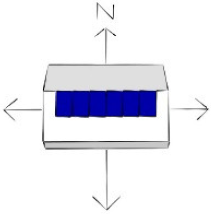
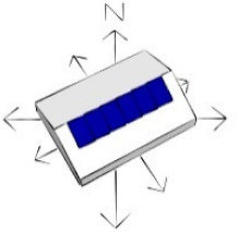
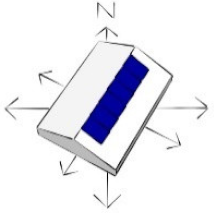
Agriculture 11 01255 i001 Agriculture 11 01255 i002 Agriculture 11 01255 i003 Agriculture 11 01255 i004
slope: 25°
orientationN―SNW―SENW―SEW―E
azimuth180°330°150°300°120°270°90°
PPV,STC 6 kW 6 kW 6 kW3 kW3 kW
PPV,STC 1 1 kW5 kW2 kWp4 kW
Wall-mounted
systems
Agriculture 11 01255 i005 Agriculture 11 01255 i006 Agriculture 11 01255 i007 Agriculture 11 01255 i008
slope: 90°
orientationN―SNW―SENW―SEW―E
azimuth180°330°150°300°120°270°90°
PPV,STC 6 kW 6 kW 6 kW3 kW3 kW
1 Additional energy yield estimation dividing the PPV,STC between the two roofs.
Table 3. Summary of monthly values for the year-round cultivation concept in Borlänge, Sweden.
Monthly Average ValuesJanFebMarAprMayJunJulAugOctNovDec
Ambient temperature-Ta (°C)−4.8−4.4−0.94.710.014.116.715.111.35.51.4
Daily global horizontal irradiation—Hh (kWh·m−2·d−1)0.30.92.33.94.85.34.83.72.41.10.4
Daily Light Integral-DLIsun (mol·m−2·d−1)2.26.617.128.334.838.835.226.917.58.12.5
Diffuse to global horizontal irradiance ratio (Gd/Gh)67%59%44%41%41%40%41%43%46%51%64%
Indoor cultivation with sole-source LED lighting 1 Agriculture 11 01255 i009 Agriculture 11 01255 i010
Greenhouse cultivation with supp. LED lighting Agriculture 11 01255 i011 Agriculture 11 01255 i012
Outdoor cultivation with natural light Agriculture 11 01255 i013
1 Arrows and shaded regions indicate the months when each cultivation type could be used.
Table 4. Parametric comparison of the estimated daily supplementary lighting and corresponding electric energy consumption for a 181 days greenhouse cultivation from February to May and from August to October in Borlänge, Sweden.
Greenhouse parametersOn−off lighting control protocol
 Minimum PAR level (PPFDthreshold)100 µmol·m−2·s−1200 µmol·m−2·s−1300 µmol·m−2·s−1
 Transmittance (τh, PAR)40%55%70%40%55%70%40%55%70%
 Daily supplementary lighting requirements
(DLIlamps, mol·m−2·d−1)
2.92.52.38.47.36.315.612.912.0
Lamps’ photosynthetic photon efficacy (PPE)Yearly 1 lighting energy consumption (Eel, lamps, kWh·m−2·yr−1)
 PPE = 2 µmol·J−1736358210183159393325302
 PPE = 2.75 µmol·J−1534643153133116286236219
 PPE = 3.5 µmol·J−142363312010491225185172
Greenhouse parametersAdaptive lighting control protocol
 Minimum PAR light level (PPFDthreshold)100 µmol·m−2·s−1200 µmol·m−2·s−1300 µmol·m−2·s−1
 Transmittance (τh, PAR)40%55%70%40%55%70%40%55%70%
 Daily supplementary lighting requirements
(DLIlamps, mol·m−2·d−1)
2.22.01.85.85.04.510.59.08.1
Lamps’ photosynthetic photon efficacy (PPE)Yearly 1 lighting energy consumption (Eel, lamps, kWh·m−2·yr−1)
 PPE = 2 µmol·J−1544946146126114264227204
 PPE = 2.75 µmol·J−13936341069183192165148
 PPE = 3.5 µmol·J−1312827837265151130116
1 Calculation made for 180 greenhouse cultivation days from 1 February to 20 May and from 20 August to 31 October.
Table 5. Yearly specific energy yields for the different greenhouse integrated PV systems in Borlänge, Sweden.
Roof-Mounted (25°)Wall-Mounted (90°)
Greenhouse Integrated PV Systemsabcdefwxyz
Yearly PV specific energy yield (Erel,PV, kWh·kW−1·yr−1)904888823825743708745732648484
Publisher’s Note: MDPI stays neutral with regard to jurisdictional claims in published maps and institutional affiliations.

