Prediction of Wheat Stripe Rust Occurrence with Time Series Sentinel-2 Images

Abstract

Wheat stripe rust has a severe impact on wheat yield and quality. An effective prediction method is necessary for food security. In this study, we extract the optimal vegetation indices (VIs) sensitive to stripe rust at different time-periods, and develop a wheat stripe rust prediction model with satellite images to realize the multi-temporal prediction. First, VIs related to stripe rust stress are extracted as candidate features for disease prediction from time series Sentinel-2 images. Then, the optimal VI combinations are selected using sequential forward selection (SFS). Finally, the occurrence of wheat stripe rust in different time-periods is predicted using the support vector machine (SVM) method. The results of the features selected demonstrate that, before the jointing period, the optimal VIs are related to the biomass, pigment, and moisture of wheat. After the jointing period, the red-edge VIs related to the crop health status play important roles. The overall accuracy and Kappa coefficient of the prediction model, which is based on SVM, is generally higher than those of the k-nearest neighbor (KNN) and back-propagation neural network (BPNN) methods. The SVM method is more suitable for time series predictions of wheat stripe rust. The model obtained accuracy based on the optimal VI combinations and the SVM increased over time; the highest accuracy was 86.2%. These results indicate that the prediction model can provide guidance and suggestions for early disease prevention of the study site, and the method combines time series Sentinel-2 images and the SVM, which can be used to predict wheat stripe rust.

1. Introduction

Wheat stripe rust is a devastating airborne disease caused by Puccinia striiformis f. sp. tritici (Pst) [1]. Stripe rust delays wheat growth, noticeably affects the wheat yield and quality, and can result in yield losses of more than 30% in epidemic years if field mismanagement and unfavorable weather conditions occur [2,3,4,5]. Stripe rust occurs in more than 60 countries globally, and the disease-affected area has been expanding in recent years [6]. Due to the extensive damage and rapid spread of wheat stripe rust, it is urgent to develop a timely and efficient disease control method to ensure food security; specifically, high-precision wheat stripe rust prediction methods that are applicable to large areas are needed [4,7,8].

Traditional methods typically use meteorological data to predict the occurrence of crop diseases, as spore germination, infection, and survival require suitable environmental conditions, such as suitable temperatures, humidity conditions, and rainfall. Several scholars have developed prediction models by combining weather forecasting and microclimate measurement data [9,10,11]. Jarroudi et al. used a Monte Carlo simulation method to determine the optimal ranges of rainfall, relative humidity, and air temperature that are favorable for wheat stripe rust occurrence and established two weather-based models to predict stripe rust severity in Morocco and Luxembourg [12,13]. Allen–Sader et al. used numerical weather prediction (NWP) meteorological forecast data to extract temperature, humidity, and solar radiation data and combined environmental suitability models, constructing disease early warning systems (EWS) for assessing the risks of stripe rust in Ethiopia [14]. Meyer et al. used the UK Met Office’s Unified Model to extract global meteorological data, combined with a Lagrangian dispersion model, successfully predicting dispersal routes and severity of stripe rust [15]. Models driven by meteorological data demonstrate good performances in representing disease occurrence trends for long-time-series disease predictions. However, the accuracy of these models is influenced by meteorological parameters, and their spatial scales are relatively coarse.

Remote sensing is an effective method used to obtain continuous spatiotemporal data and has been increasingly used for large-scale monitoring and prediction of crop diseases [16,17,18,19]. Zheng et al. used hyperspectral data to simulate Sentinel-2 satellite image bands and developed the red-edge disease stress index (REDSI) to monitor wheat stripe rust successfully [20]. Dutta et al. used RESOURCESAT-1 (IRS-P6) satellite data to extract the normalized difference vegetation index (NDVI) and land surface water index (LSWI) and established a prediction model for stripe rust occurrence, based on the spectral profile analysis method [21]. Du et al. used RapidEye satellite data to extract crop growing conditions and combined three classification methods (the maximum likelihood classifier (MLC), support vector machine (SVM), and random forest (RF)) to predict wheat stripe rust in the filling period; the results showed that all three methods achieved high accuracies [22]. Existing research on remote sensing-based crop disease prediction mostly established disease prediction models by extracting remote sensing features within a single period and predicted disease occurrence at regional scales to improve the spatial prediction accuracy. Since wheat stripe rust occurs almost throughout the entire wheat growth period, a multi-temporal prediction method is urgently needed to guide disease prevention and control measures throughout the entire growing period.

Several researchers have used time series remote sensing images to develop prediction methods for crop diseases. Pryzant et al. used time series moderate-resolution imaging spectroradiometer (MODIS) data throughout the wheat growing season and combined it with convolutional and long short-term memory networks, presented a framework for predicting stripe rust, and achieved a good result comparing it with the use of Triangular Vegetation Index (TVI), NDVI, the Chlorophyll Absorption in Reflectance Index (CARI), and other traditional vegetation indices [23]. Dong et al. used multi-source remote sensing data (MODIS, Landsat 8 and Sentinel-2 images) to extract the plant senescence reflectance index (PSRI), the red-edge vegetation stress index (RVSI), and land surface temperature (LST), and established a multi-period prediction model based on SVM, in order to predict stripe rust severity in China [24].

The damage caused by wheat stripe rust and the associated morphological and physiological characteristics changes over time as the disease develops [2,3,4,25]. In the early infection period, chlorotic spots are formed on the leaf surface, followed by yellow uredinia, and large numbers of uredinia forms stripes. In the later infection period, due to the destruction of the cell structure and lack of nutrients and water, infected wheat wilts and forms many necrotic streaks. These symptoms only appear after the jointing period as the disease worsens [3,4]. The changes in the pigment, biomass, moisture, and other characteristics of wheat caused by diseases can influence its multi-band reflectance. Vegetation indices (VIs) obtained from the combination of spectral bands are often used to characterize these changes [26]. Salarux et al. successfully characterized algal bloom biomass in the field by using NDVI, which was established by the normalized difference between the near-infrared and red band [27,28]. Fensholt et al. established the shortwave infrared water stress index (SIWSI), which uses near-infrared and shortwave infrared bands based on MODIS data, and successfully estimated vegetation canopy water stress in a semiarid Sahelian environment [29]. The SIWSI has been widely used to characterize water content changes, such as the detection of variations in the land-surface moisture and vegetation moisture statuses in the semiarid Sahel [30]. Merzlyak et al. used the red-edge band and visible light band to create the plant senescence reflectance index (PSRI) based on a spectrophotometer; PSRI proved to be sensitive to fruit pigment changes in greenhouses and the natural environment [31]. Combining time series remote sensing images and agronomy can provide accurate information on the occurrence and development of diseases. In particular, the filling period is an important wheat-growing period that affects the wheat yield. Infections during this period cause significant wheat yield and quality losses [4]. However, most of the existing remote sensing prediction methods for wheat yellow rust depend on the characteristics of a single period to predict the occurrence of the disease [20,21,22], and few studies have considered the differences of these characteristics among different periods [23,24]. In this study, we used time series remote sensing images to establish a prediction model and predict the occurrence of wheat stripe rust in the filling period. Time series Sentinel-2 images were adopted in this study. The objectives of this study were (1) to extract the optimal VI combinations at different time periods, to be used to predict wheat stripe rust during the filling period, and (2) to evaluate the performance of the wheat stripe rust prediction model, based on the SVM method.

2. Materials and Methods

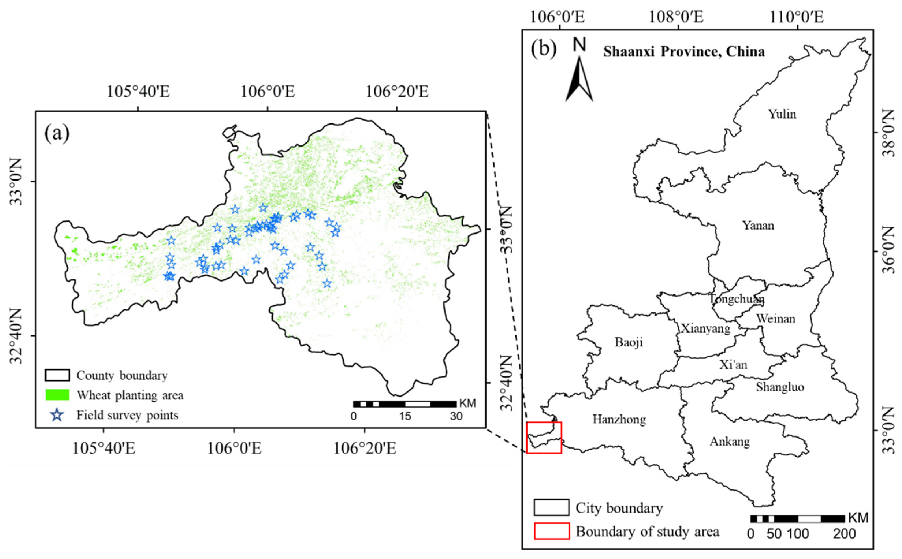
2.1. Study Site

The study site is located in Ningqiang County, Hanzhong City, Shaanxi Province, China (32°27′06″–33°12′42″ N, 105°20′10″–106°35′18″ E) (Figure 1). The county is located in the southwest corner of Shaanxi Province. It is the boundary between the over-summering and over-wintering regions of the Chinese wheat stripe rust pathogen [32,33]. The annual average temperature and precipitation of the county are 13 °C, and 1812.2 mm, respectively [34]. Low-temperature and high-humidity environmental conditions increase the occurrence of wheat stripe rust in this region [20,35]. Stripe rust is the major wheat disease in the county and severely affected the local crops in 2018. The wheat in this county is usually sown in early October, and enters the regreening period in the subsequent early March, in which the peak period of stripe rust begins to occur. In mid-May, wheat enters the filling period, which is the serious period of stripe rust damage, and is harvested in mid-June.

2.2. Data Acquisition and Preprocessing

During the field survey (11–12 May 2018), a total of 58 plots were identified and the occurrence degree of stripe rust in each plot was recorded. The geographical information (latitude and longitude) of each plot was also recorded using a submeter-precision handheld global positioning system (GPS) receiver. Meanwhile, the growing stage was obtained from the local plant protection station. The 10 × 10 m plot was selected at a 20 × 20 m spatial extent, where the disease was relatively uniform to match the plots and satellite image pixels. Next, five 1 m × 1 m quadrats were selected at each plot, and ten leaves were randomly selected at each quadrat. The severity level of stripe rust on the leaves was divided into 9 categories (0%, 1%, 5%, 10%, 20%, 40%, 60%, 80%, and 100%). The severity level was assessed according to the percentage of the infected spot area in the total leaf area and was performed by one professional. Then, the disease index (DI) values of the quadrats were calculated using the following equation:

$$DI=F\times D\times 100, D=\frac{{\displaystyle \sum (i\times l_i)}}{L}, F=\frac{l}{L}$$

(1)

where F is the incidence of quadrats and represents the percentage of the number of infected leaves in the total number of investigated leaves, D is the average severity of the quadrats, i is the severity level, l_i is the total number of leaves associated with each severity level, L is the total number of leaves investigated, and l is the number of infected leaves.

The average DI value of the five quadrats represents the disease occurrence degree of the corresponding plot. The disease occurrence degree reflects the overall occurrence of stripe rust at the plot. The severity level, DI, and disease occurrence degree calculations for wheat stripe rust were based on monitoring and forecasting rules of wheat stripe rust (GB/T15795-2011) [20]. The disease occurrence degree of plot was grouped into two classes for constructing the prediction model. The classes included healthy (disease occurrence degree ≤ 5) and diseased (disease occurrence degree > 5), and were represented by values 1 and 2, respectively. If the plot occurs seriously, the plot disease occurrence degree obviously exceeds the threshold range; we directly marked this as diseased.

Sentinel-2 satellite images were downloaded from the European Space Agency Sentinels Scientific Date Hub (https://scihub.copernicus.eu/ accessed on 15 October 2021) on the following five dates: March 13 (regreening period), March 28 (standing period), April 02 (jointing period), April 22 (heading period), and April 27 (flowering period) of 2018. The remote sensing images were preprocessed for atmospheric corrections using the Sen2cor module, and resampled to 10 m using the resampling tool in the Sentinel Application Platform software (SNAP). The spatial distribution of wheat in the study area was extracted using the decision tree method and multi-temporal phenological information methods [36,37,38]. We used 58 field survey plots to verify the accuracy of extracted wheat area, 55 plots were correctly extracted, and the overall validation accuracy of 95% was obtained.

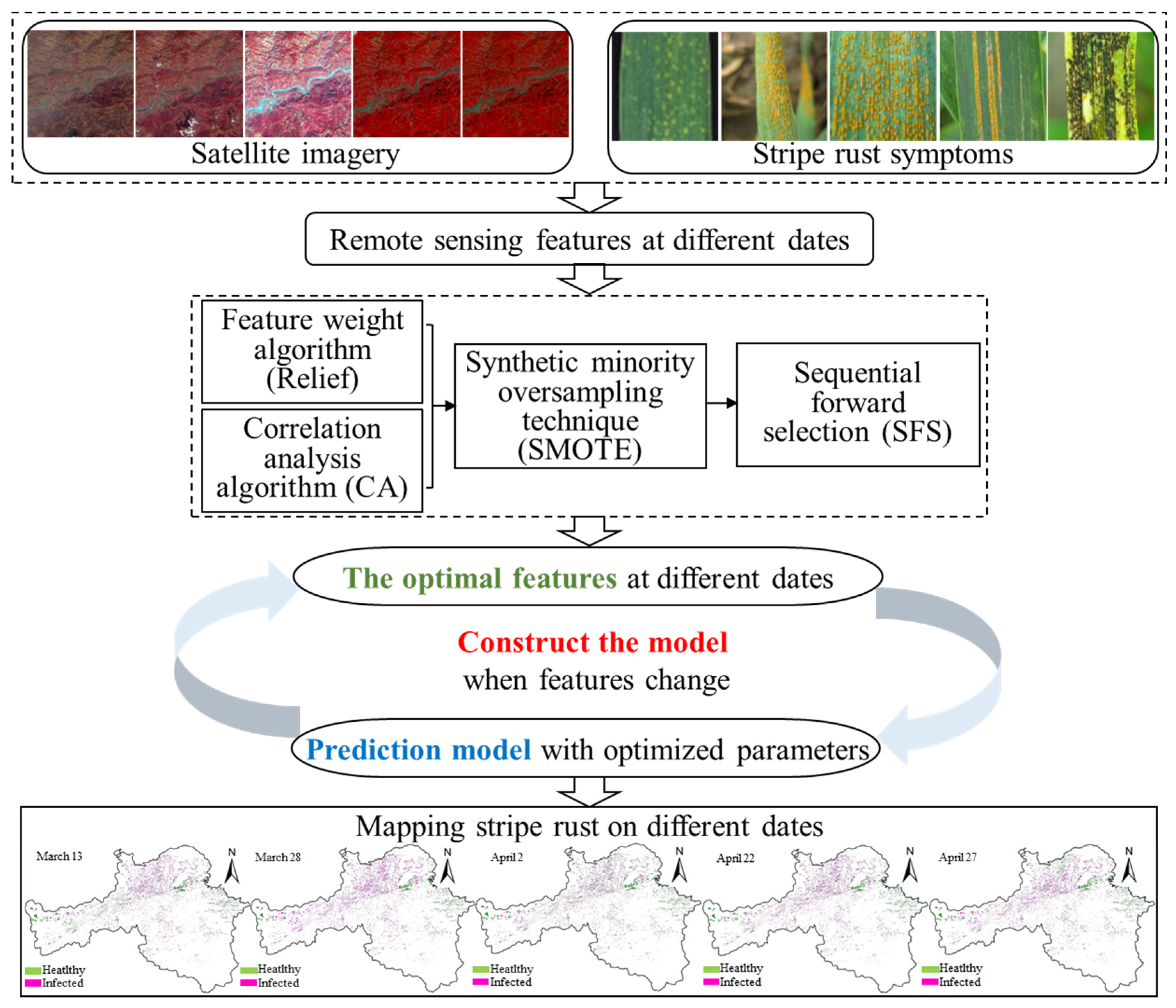
2.3. Prediction of Wheat Stripe Rust by Using Time Series Remote Sensing Images

The establishment of stripe rust prediction model included two steps. First, the time series satellite images were used to extract the remote sensing features as candidate features. The optimal feature combination in each time period was determinized using the feature selection. Then, the stripe rust prediction model was established using the SVM method. The occurrence of stripe rust was predicted with the change of the optimal feature combinations and model parameters. Figure 2 shows a flowchart of the wheat stripe rust prediction using time series Sentinel-2 images.

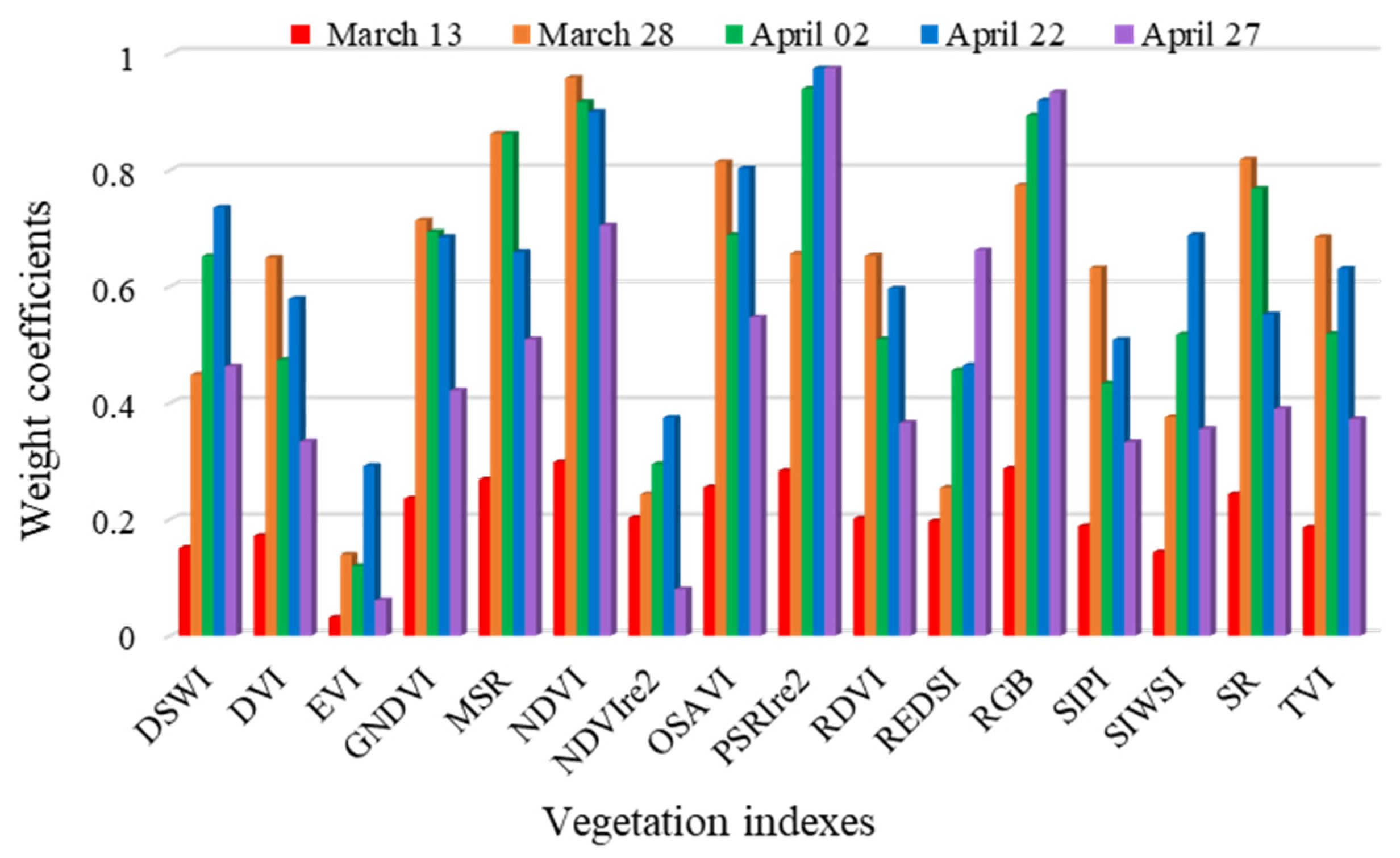
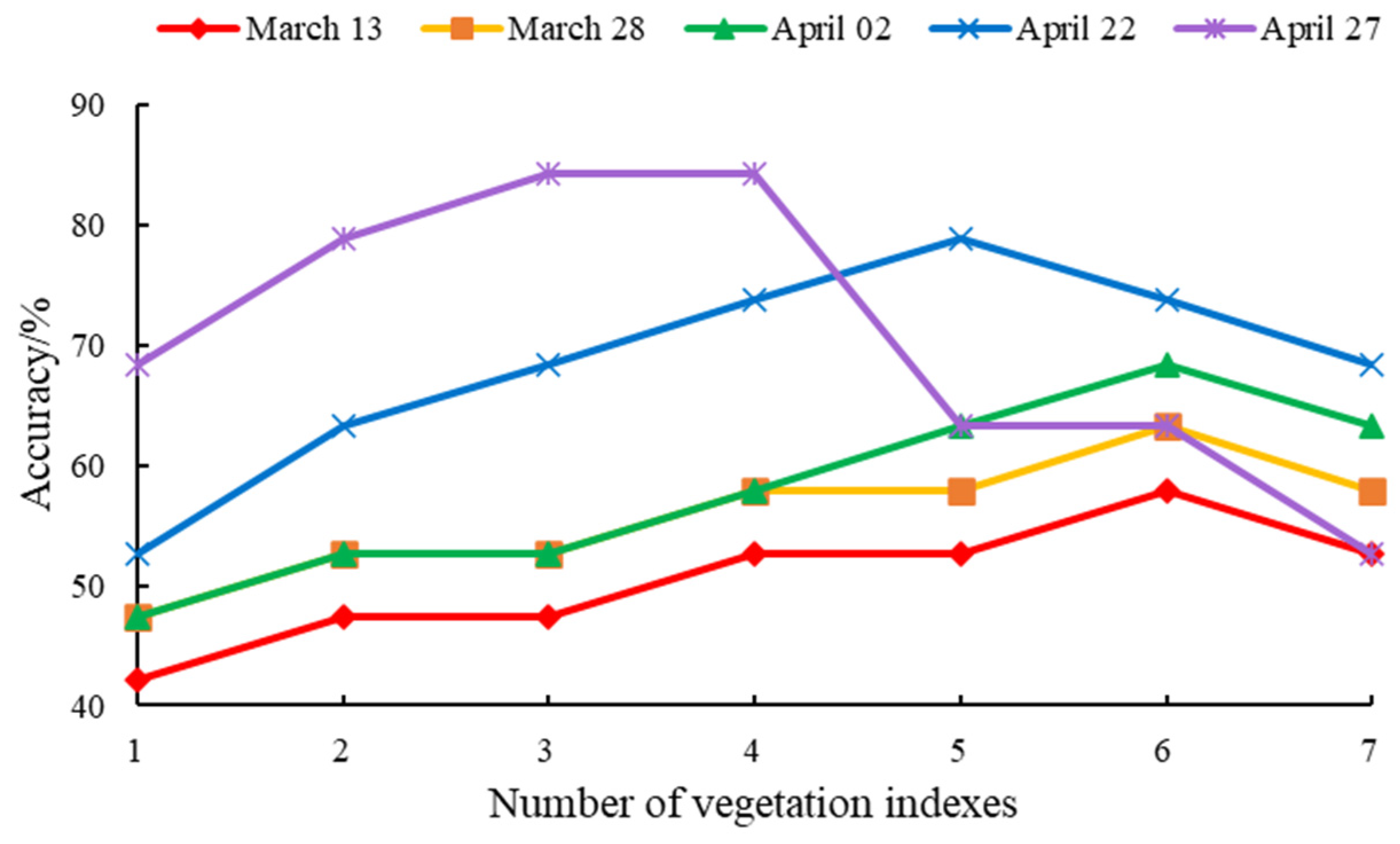
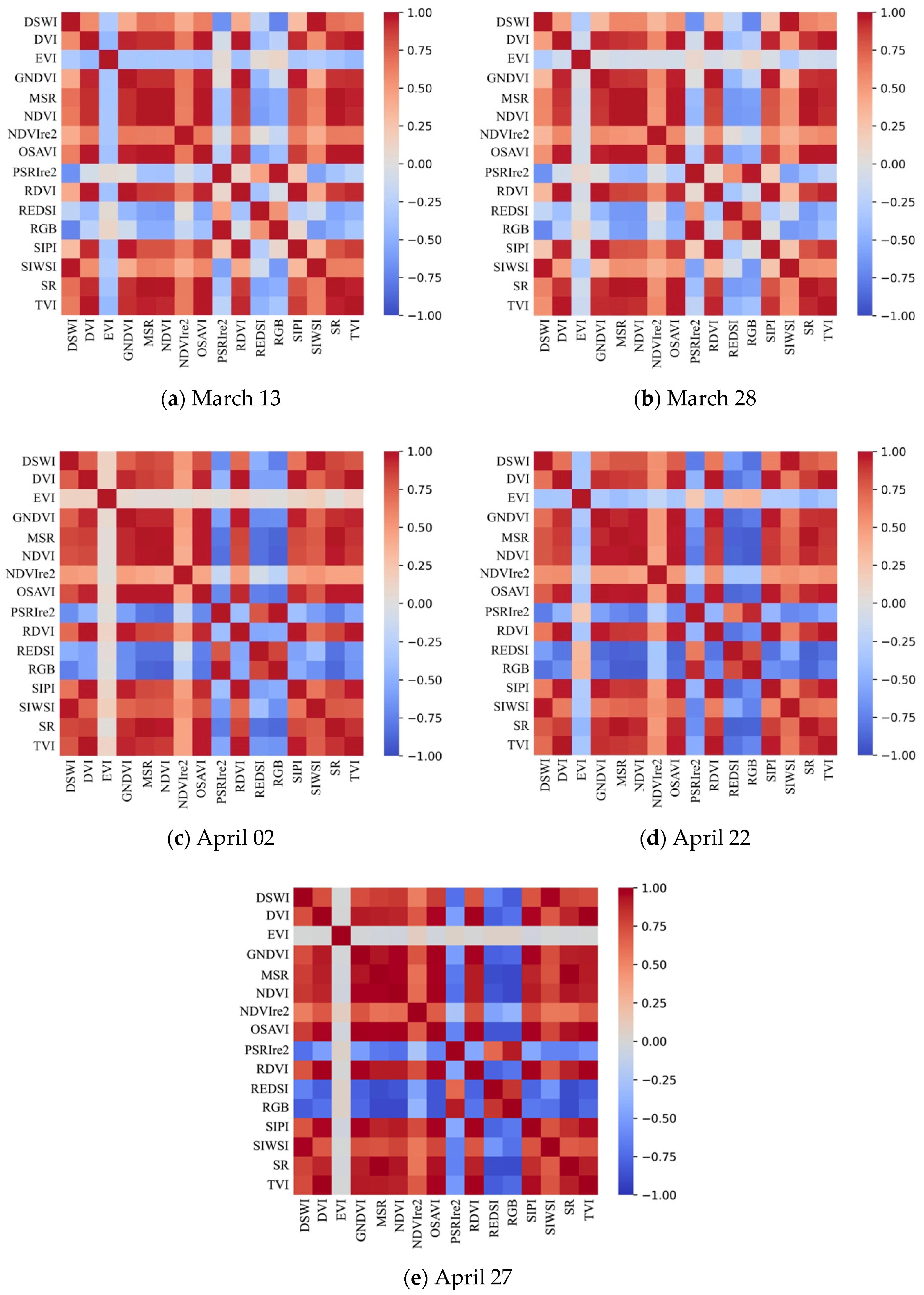
2.3.1. Selection of Optimal Vegetation Indice Combinations

The primary step in constructing the wheat strip rust prediction model was to extract the optimal VI combinations characterizing the occurrence and development of the disease at different time periods. Before the feature extraction, the effects of stripe rust on wheat at different growing conditions were evaluated. A total of 16 VIs were selected to categorize the changes into pigment, biomass, water, and other growing conditions of wheat under stripe rust stress as candidate features (Table 1). The similarity of VIs, correlation between VIs and stripe rust, and the differences in the stripe rust effects with growing conditions impact the accuracy of prediction models. To overcome these effects and improve the accuracy, feature extraction using the candidate features was performed to determine the optimal VI combinations at different time periods.

First, the correlation analysis was used to measure the correlation coefficients of the VIs. The weighted coefficients of the VIs and the occurrence of stripe rust in each time period were calculated using a relief algorithm. The relief algorithm is a feature weight algorithm that gives different weight coefficients to features by calculating the correlations between features and categories [39,40]. The high weight coefficient indicates that the feature has a strong ability to distinguish different categories. To minimize similarity among the VIs, the VIs with the highest weight coefficient was used as a benchmark, and the other VIs with correlation coefficients greater than 0.9 were removed [41]. All VIs were processed in the same manner.

Then, the sequential forward selection (SFS)-based SVM was used to obtain the optimal VI combinations. SFS is a bottom-up search method that selects one feature, adds a feature subset at a given time, and inputs an SVM to calculate the classification accuracies of different feature combinations [42]. The feature subset with the highest accuracy is the optimal combination. After removing the similarities from the Vis, they were added in descending order of the weight coefficients, as inputs of the SVM. The field survey samples were used to train the SVM and test the accuracies of different VI combinations in extracting the optimal VI combinations of different time periods. Due to the imbalance between the healthy and diseased sample categories, the synthetic minority oversampling technique (SMOTE) algorithm was used to balance the sample categories and prevent overfitting during SFS. SMOTE is an oversampling technique that reduces the imbalance between categories by artificially synthesizing new minority samples [43,44,45,46]. The 58 samples were divided into training and validation sets using a 7:3 ratio. The training samples contained 15 healthy samples and 24 wheat stripe rust-infected samples, and the training samples were balanced using the SMOTE algorithm. The VI combinations with the highest accuracy in each time period were considered as the optimal remote sensing feature set for that period.

Table 1. Vegetation indices used for stripe rust predictions. These vegetation indices were used as candidate features.

Vegetation Indices Definition	Formula	Correlation
Normalized difference Vegetation index, NDVI [27]	$(R_{NIR}-R_R)/(R_{NIR}+R_R)$	LAI, biomass
Normalized difference vegetation Index red-edge2, NDVIre2 [47]	$(R_{NIR}-R_{\mathrm{Re}2})/(R_{NIR}+R_{\mathrm{Re}2})$	LAI, biomass
Green normalized difference Vegetation index, GNDVI [48]	$(R_{NIR}-R_G)/(R_{NIR}+R_G)$	Pigment concentration
Ratio of red and green, RGB [49]	$R_R/R_G$	Leaf pigment content
Modified simple ratio index, MSR [50]	$(R_{NIR}/R_R-1)/(\sqrt{(R_{NIR}+R_R)}+1)$	Vegetation status
Simple ratio index, SR [51]	$R_{NIR}/R_R$	Photosynthetic area
Enhanced vegetation index, EVI [52]	$2.5(R_{NIR}-R_R)/(R_{NIR}+6R_R-0.5R_B+1)$	Sensitive to canopy
Renormalized difference Vegetation index, RDVI [53]	$(R_{NIR}-R_R)/\sqrt{(R_{NIR}+R_R)}$	Vegetation coverage
Structural independent Pigment index, SIPI [54]	$(R_{NIR}-R_B)/(R_{NIR}+R_B)$	Pigment content
Difference vegetation index, DVI [55]	$(R_{NIR}-R_R)$	Vegetation coverage
Optimized soil-adjusted Vegetation index, OSAVI [56]	$(R_{NIR}-R_R)/(R_{NIR}+R_R+0.16)$	Minimize brightness-related soil effects
Plant senescence reflectance Index, PSRI2 [31]	$(R_R-R_G)/R_{\mathrm{Re}2}$	Pigment content, vegetation health
Red-edge disease stress Index, REDSI [20]	$((705-665)(R_{\mathrm{Re}3}-R_R)-(783-665)(R_{\mathrm{Re}1}-R_R))/(2R_R)$	Sensitive to stripe rust
Triangular vegetation index, TVI [57]	$0.5[120(R_{NIR}-R_G)-200(R_R-R_G)]$	Vegetation status
Shortwave infrared water Stress index, SIWSI [29]	$(R_{NIR}-R_{SWIR})/(R_{NIR}+R_{SWIR})$	Water status
Disease water stress index, DSWI [58]	$(R_{NIR}+R_G)/(R_{SWIR}+R_R)$	Water status

Table 1. Vegetation indices used for stripe rust predictions. These vegetation indices were used as candidate features.

Vegetation Indices Definition	Formula	Correlation
Normalized difference Vegetation index, NDVI [27]	$(R_{NIR}-R_R)/(R_{NIR}+R_R)$	LAI, biomass
Normalized difference vegetation Index red-edge2, NDVIre2 [47]	$(R_{NIR}-R_{\mathrm{Re}2})/(R_{NIR}+R_{\mathrm{Re}2})$	LAI, biomass
Green normalized difference Vegetation index, GNDVI [48]	$(R_{NIR}-R_G)/(R_{NIR}+R_G)$	Pigment concentration
Ratio of red and green, RGB [49]	$R_R/R_G$	Leaf pigment content
Modified simple ratio index, MSR [50]	$(R_{NIR}/R_R-1)/(\sqrt{(R_{NIR}+R_R)}+1)$	Vegetation status
Simple ratio index, SR [51]	$R_{NIR}/R_R$	Photosynthetic area
Enhanced vegetation index, EVI [52]	$2.5(R_{NIR}-R_R)/(R_{NIR}+6R_R-0.5R_B+1)$	Sensitive to canopy
Renormalized difference Vegetation index, RDVI [53]	$(R_{NIR}-R_R)/\sqrt{(R_{NIR}+R_R)}$	Vegetation coverage
Structural independent Pigment index, SIPI [54]	$(R_{NIR}-R_B)/(R_{NIR}+R_B)$	Pigment content
Difference vegetation index, DVI [55]	$(R_{NIR}-R_R)$	Vegetation coverage
Optimized soil-adjusted Vegetation index, OSAVI [56]	$(R_{NIR}-R_R)/(R_{NIR}+R_R+0.16)$	Minimize brightness-related soil effects
Plant senescence reflectance Index, PSRI2 [31]	$(R_R-R_G)/R_{\mathrm{Re}2}$	Pigment content, vegetation health
Red-edge disease stress Index, REDSI [20]	$((705-665)(R_{\mathrm{Re}3}-R_R)-(783-665)(R_{\mathrm{Re}1}-R_R))/(2R_R)$	Sensitive to stripe rust
Triangular vegetation index, TVI [57]	$0.5[120(R_{NIR}-R_G)-200(R_R-R_G)]$	Vegetation status
Shortwave infrared water Stress index, SIWSI [29]	$(R_{NIR}-R_{SWIR})/(R_{NIR}+R_{SWIR})$	Water status
Disease water stress index, DSWI [58]	$(R_{NIR}+R_G)/(R_{SWIR}+R_R)$	Water status

2.3.2. Establishment and Performance Test of the Wheat Stripe Rust Prediction Model

Subsequently, the SVM method was used to establish a prediction model for wheat stripe rust [59,60,61]. The prediction of stripe rust was accomplished by inputting the optimal VI combinations and model parameters. The occurrence of stripe rust in each pixel was predicted, and the maps of stripe rust occurrence in each time period were outputted by the prediction model. In the SVM method, the main idea was to determine an optimal decision boundary and maximize the distance between the two kinds of samples as much as possible [62]. Radial basis function (RBF) was used as the kernel function of SVM classification, which shows superior performance in the case of online inseparability [63]. SVM method contained two important parameters, namely, the cost constraint (C) and gamma (γ). C is the tolerance to error. γ is a parameter of RBF function. It implicitly determines the distribution of data after mapping to the new feature space. Higher gamma indicates fewer support vectors. The number of support vectors affects the speed of training and prediction. The balanced field survey samples by SMOTE algorithm and a grid search (GS) method were used to optimize C and γ and train the model in each period [64]. The 10-fold cross validation method was used to determine the performance of the model in predicting the occurrence of stripe rust [65]. This method split the 58 samples into 10 folds; one of them was selected as the validation set, and the remaining folds for model training; 10 iterations were performed so that each fold was used as the validation set and the rest as the training set. Finally, the average accuracy was calculated as the final accuracy. The overall accuracy (OA), producer accuracy (PA), user accuracy (UA), and kappa coefficient of the prediction model in each period were used to assess the performance of the prediction model (Table 2) [66]. The OA can directly reflect the proportion of correct classifications. The high OA indicates that the model has good overall classification effect. The kappa coefficient is a metric used to measure the agreement between the predicted results and actual results. The high Kappa coefficient indicates that the model has strong consistency. The PA and UA indicate the accuracies of individual categories.

The SVM method was compared with the k-nearest neighbor (KNN) and the back-propagation neural network (BPNN) methods [67]. The KNN method was a majority voting method, based on the closest k training samples in the feature space. The performance of KNN is affected by the parameter, k [68]. The GS method was used to optimize k in each time-period. The BPNN method was designed to minimize the total error (or average error) between actual output and desired output, through optimizing the weights of neural network. The network was composed of the input layer, output layer, and hidden layer [67]. The performance of BPNN is affected by the number of layers, which is determined by the dimension of the input features and category of the output [69].

The SVM-, KNN-, and BPNN-based prediction models were developed using MATLAB 2018a software. Among them, the SVM method and the optimization of parameter C and γ were realized by LibSVM Toolbox; KNN was realized by Statistics and Machine Learning Toolbox and BPNN was realized by Deep Learning Toolbox.

The influences of the VIs and parameters on the performance of the prediction model were considered. The similarity among the VIs is the correlation between the VIs and the occurrence of stripe rust, and the differences in VIs among different time periods due to stripe rust were considered. Then, the optimal VI combinations in different time periods were extracted as the model inputs. We also optimized the model parameters in different time periods by the GS method. Finally, the stripe rust prediction model was realized with the VI combinations and model parameters and changed over time.

Table 2. Summary of the accuracy measures applied for the prediction models.

Name	Formula	References
Overall accuracy, OA	$U{A}_i=x_{ii}/x_{i+}$	[70]
Producer accuracy, PA	$P{A}_i=x_{ii}/x_{+i}$	[70]
User accuracy, UA	$OA={\displaystyle \sum _{i=1}^m{x}_{ii}}/x$	[70]
Kappa coefficient	$Kappa=(OA-EA)/(1-EA), EA={\displaystyle \sum _{i=1}^m\frac{x_{i+}}{x}}\frac{x+i}{x}$	[71]

Note: i is the wheat category in this study; i = 1 and i = 2 indicate healthy and stripe rust-infected wheat, respectively. UA_i, PA_i, and OA indicate the user accuracy of category i, the producer accuracy of category i, and the overall accuracy of the prediction model, respectively. x_ii, x_i+, x_+i, x denote the correct prediction number of category i, the total number of category i samples obtained from the ground-truth survey, the total number of category i samples obtained from the prediction model, and the total prediction number of all categories, respectively. m is the number of categories, which equals 2 in this study.

Table 2. Summary of the accuracy measures applied for the prediction models.

Name	Formula	References
Overall accuracy, OA	$U{A}_i=x_{ii}/x_{i+}$	[70]
Producer accuracy, PA	$P{A}_i=x_{ii}/x_{+i}$	[70]
User accuracy, UA	$OA={\displaystyle \sum _{i=1}^m{x}_{ii}}/x$	[70]
Kappa coefficient	$Kappa=(OA-EA)/(1-EA), EA={\displaystyle \sum _{i=1}^m\frac{x_{i+}}{x}}\frac{x+i}{x}$	[71]

Note: i is the wheat category in this study; i = 1 and i = 2 indicate healthy and stripe rust-infected wheat, respectively. UA_i, PA_i, and OA indicate the user accuracy of category i, the producer accuracy of category i, and the overall accuracy of the prediction model, respectively. x_ii, x_i+, x_+i, x denote the correct prediction number of category i, the total number of category i samples obtained from the ground-truth survey, the total number of category i samples obtained from the prediction model, and the total prediction number of all categories, respectively. m is the number of categories, which equals 2 in this study.

3. Results

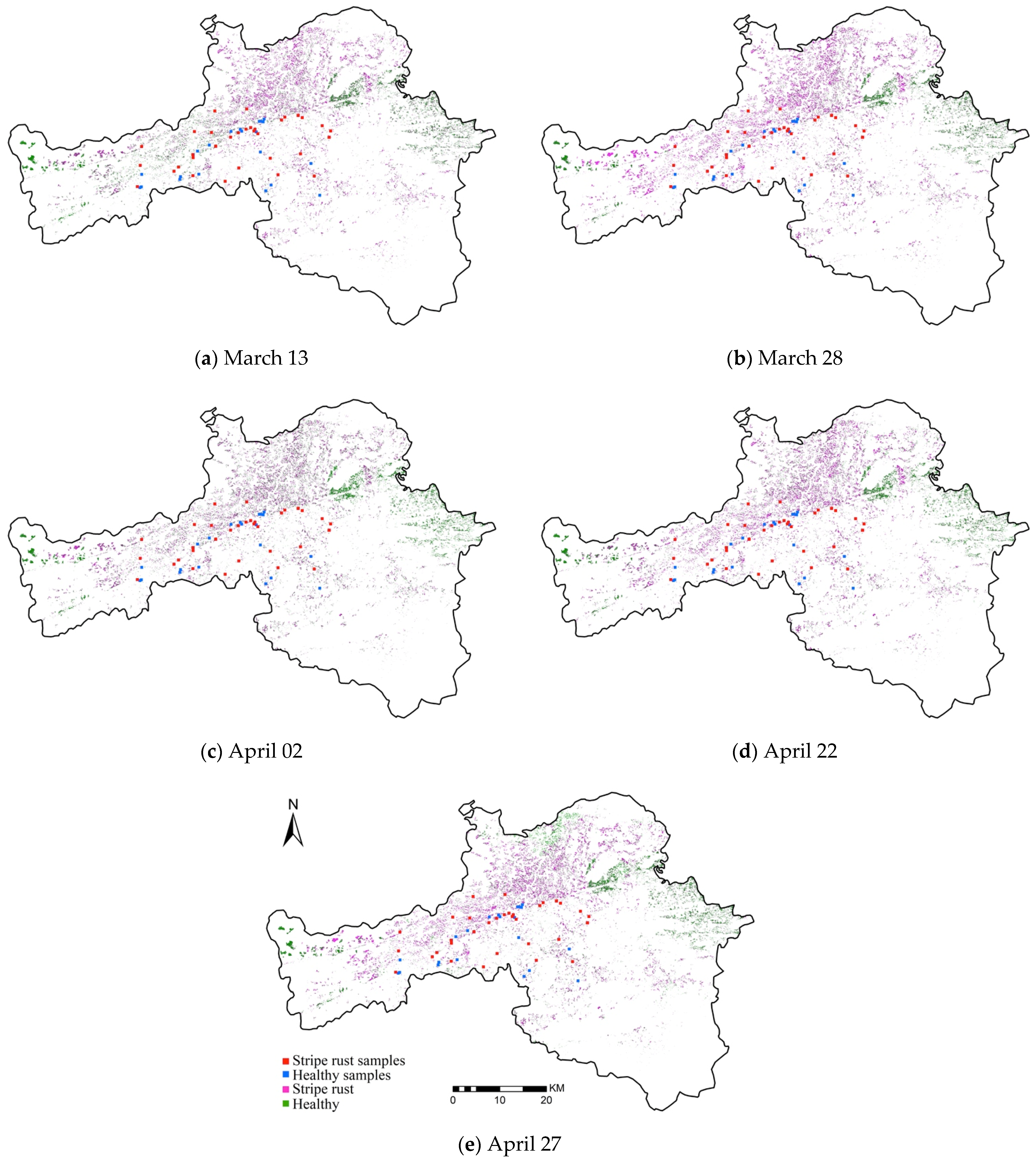
3.1. Time Series Remote Sensing Stripe Rust Feature Extraction

The first step of constructing the prediction model was to extract the optimal VI combinations representing different time periods. The candidate features included 16 Vis, which can characterize changes in the growing conditions of wheat under stripe rust stress (Table 1). First, the correlations among the VIs at five dates were analyzed using a correlation analysis; the results are shown in Figure 3. The results demonstrated that the NDVI and green normalized the difference in the vegetation index (GNDVI), modified the simple ratio index (MSR), optimized the soil-adjusted vegetation index (OSAVI), and the simple ratio index (SR) showed high positive correlations on five dates. The DSWI and SIWSI had high positive correlations on five dates, and the ratio of red and green (RGB) and PSRIre2 had high positive correlations on five dates. The overall results indicated high correlations among the candidate features.

The relief algorithm was used to calculate the weight coefficients between the VIs and the occurrence of wheat stripe rust at the five studied dates to minimize the similarity among VIs. The results are shown in Figure 4, indicating that the NDVI, RGB, and PSRIre2 had higher weight coefficients than the other VIs at the five studied dates. The weight coefficients of RGB, PSRIre2, and REDSI increased over time. The NDVI had the highest weight coefficients on March 13 and March 28. PSRIre2 had the highest weight coefficients on April 02, April 22, and April 27, and the enhanced vegetation index (EVI) had the smallest weight coefficients at the five studied dates. If the correlation coefficient between two VIs was greater than 0.9, the VIs with the smaller weight was discarded. The selected VIs are shown in

Table 3. Vegetation indice combinations after similarity removal at five dates. Each row represents the vegetation indice combinations after the similarity removal on the corresponding date.

Date	Vegetation Indices Combination
March 13	NDVI, RGB, NDVIre2, RDVI, REDSI, DSWI, EVI
March 28	NDVI, RGB, NDVIre2, RDVI, REDSI, DSWI, EVI
April 02	PSRIre2, NDVI, NDVIre2, TVI, REDSI, DSWI, EVI
April 22	PSRIre2, NDVI, NDVIre2, TVI, REDSI, DSWI, EVI
April 27	PSRIre2, NDVI, NDVIre2, TVI, REDSI, DSWI, EVI

. Table 3 shows that the selected VIs were the same on March 13 and March 28, and the same VIs were selected on April 02, April 22, and April 27. However, the weight coefficients of the VIs differed between the five studied dates.

Finally, the accuracies of different VI combinations were calculated using SFS to extract the optimal VI combinations of the five studied dates. The training samples were balanced using the SMOTE algorithm. The results obtained before and after the SMOTE algorithm were listed in

Table 4. The sample distribution of the original training samples and balanced training samples calculated by the synthetic minority oversampling technique (SMOTE) algorithm. The training samples were obtained from 58 field survey samples using a 7:3 ratio.

Type	Original Training Samples		Balanced Training Samples after Using SMOTE
	Number	Ratio	Number	Ratio
Healthy	15	38.5%	24	50.0%
Diseased	24	61.5%	24	50.0%
Sum	39	100%	48	100%

. The proportion of healthy samples in the balanced training set increased to 24, and the healthy and stripe rust-infected samples each accounted for 50.0%, balancing the distribution of the sample categories. Then, the new training samples were applied to the SFS-based SVM. The results in Figure 5 show that the highest accuracies on March 13 and March 28 were achieved by the combination of NDVI, RGB, NDVIre2, RDVI, REDSI, and DSWI. On April 02, the highest accuracy was achieved by combining PSRIre2, NDVI, DSWI, TVI, REDSI, and NDVIre2. On April 22, the combination achieving the highest accuracy comprised PSRIre2, NDVI, DSWI, TVI, REDSI, and NDVIre2. On April 27, the highest accuracy was achieved by combining PSRIre2, NDVI, and REDSI (

Table 5. The optimal vegetation indice combinations at five dates. Each row represents the optimal vegetation indice combinations on the corresponding date.

Date	Vegetation Indice Combinations
March 13	NDVI, REDSI, DSWI, NDVIre2, RDVI, RGB
March 28	NDVI, REDSI, DSWI, NDVIre2, RDVI, RGB
April 02	NDVI, REDSI, DSWI, NDVIre2, TVI, PSRIre2
April 22	NDVI, REDSI, DSWI, TVI, PSRIre2
April 27	NDVI, REDSI, PSRIre2

).

3.2. Establishment and Verification of the Prediction Model of Wheat Stripe Rust

After extracting the optimal VI combinations of the five stages, the SVM method was used to establish the wheat stripe rust prediction model. The parameters of prediction models are shown in

Table 6. The model parameters of the support vector machine (SVM), k-nearest neighbor (KNN), and back propagation neural network (BPNN) on (a) March 13; (b) March 28; (c) April 02; (d) April 22; and (e) April 27.

Model			Date			Parameter
						C			γ
SVM			March 13			90.5097			0.0221
			March 28			90.5097			0.3535
			April 02			2.8248			0.0441
			April 22			45.2548			0.011
			April 27			1.0			0.0625
Model			Date			Parameter
						k
KNN			March 13			5
			March 28			5
			April 02			5
			April 22			3
			April 27			3
Model			Date			The number of layers
						Input		Hidden		Output
BPNN			March 13			6		7		2
			March 28			6		7		2
			April 02			6		7		2
			April 22			5		6		2
			April 27			3		4		2

. Figure 6 shows the prediction results of stripe rust spatial distribution: on March 13, stripe rust mainly occurred in the northern part of the study area; on March 28, April 02, and April 22, the disease did not occur in the western or eastern parts of the study area; on April 27, stripe rust did not occur in the western, eastern, or northern parts of the study area.

Table 7. Prediction model validations on (a) March 13; (b) March 28; (c) April 02; (d) April 22; and (e) April 27, based on the support vector machine (SVM), k-nearest neighbor (KNN), and back propagation neural network (BPNN) methods, using the optimal vegetation indice combinations.

Date	Method		Healthy	Infected	Sum	UA	OA	Kappa
March 13	SVM	Healthy	13	11	24	54.2%	65.5%	0.280
		Infected	9	25	34	73.5%
		Sum	22	36	58
		PA	59.1%	69.4%
	BPNN	Healthy	12	12	24	50.0%	62.1%	0.208
		Infected	10	24	34	70.1%
		Sum	22	36	58
		PA	54.5%	66.7%
	KNN	Healthy	11	13	24	45.8%	58.6%	0.136
		Infected	11	23	34	67.6%
		Sum	22	36	58
		PA	50.0%	63.9%
March 28	SVM	Healthy	14	10	24	58.3%	69.0%	0.352
		Infected	8	26	34	76.5%
		Sum	22	36	58
		PA	63.6%	72.2%
	BPNN	Healthy	13	11	24	54.2%	65.5%	0.280
		Infected	9	25	34	73.5%
		Sum	22	36	58
		PA	59.1%	69.4%
	KNN	Healthy	12	12	24	50.0%	62.1%	0.208
		Infected	10	24	34	70.1%
		Sum	22	36	58
		PA	54.5%	66.7%
April 02	SVM	Healthy	15	8	23	65.2%	74.1%	0.456
		Infected	7	28	35	80.0%
		Sum	22	36	58
		PA	68.2%	77.8%
	BPNN	Healthy	14	9	23	60.9%	70.7%	0.382
		Infected	8	27	35	77.1%
		Sum	22	36	58
		PA	63.6%	75.0%
	KNN	Healthy	13	11	24	54.2%	65.5%	0.280
		Infected	9	25	34	73.5%
		Sum	22	36	58
		PA	59.1%	69.4%
April 22	SVM	Healthy	17	7	24	70.8%	79.3%	0.568
		Infected	5	29	34	85.3%
		Sum	22	36	58
		PA	77.3%	80.6%
	BPNN	Healthy	16	8	24	66.7%	75.9%	0.496
		Infected	6	28	34	82.4%
		Sum	22	36	58
		PA	72.7%	77.8%
	KNN	Healthy	15	10	25	60.0%	70.7%	0.394
		Infected	7	26	33	78.8%
		Sum	22	36	58
		PA	68.2%	72.2%
April 27	SVM	Healthy	18	4	22	81.8%	86.2%	0.707
		Infected	4	32	36	88.9%
		Sum	22	36	58
		PA	81.8%	88.9%
	BPNN	Healthy	17	6	23	73.9%	81.0%	0.601
		Infected	5	30	35	85.7%
		Sum	22	36	58
		PA	77.3%	83.3%
	KNN	Healthy	16	7	23	69.6%	77.6%	0.528
		Infected	6	29	35	82.9%
		Sum	22	36	58
		PA	72.7%	80.6%

shows the confusion matrix of the prediction results at the five studied dates, calculated by the 58 samples from wheat stripe rust field surveys on May 11 and 12, 2018. The overall accuracy and Kappa coefficient increased over time. The prediction accuracies at the five dates (March 13, March 28, April 02, April 22, and April 27) were 65.5%, 69.0%, 74.1%, 79.3%, and 86.2%, and the kappa coefficients were 0.280, 0.352, 0.456, 0.568, and 0.707, respectively.

We compared the SVM method with the KNN and BPNN methods using the same VI combinations for each time period (Table 6). The overall accuracies and Kappa coefficients of the three methods increased over time. The overall accuracies of the BPNN method on March 13, March 28, April 02, April 22, and April 27 were 62.1%, 65.5%, 70.7%, 75.9%, and 81.0%, and the overall accuracies of the KNN method were 58.6%, 62.1%, 65.5%, 70.7%, and 77.6%. The Kappa coefficients of BPNN were 0.208, 0.280, 0.382, 0.496, and 0.601, and the Kappa coefficients of KNN were 0.136, 0.208, 0.280, 0.394, and 0.528, respectively. For three methods, the accuracy and Kappa coefficient of the SVM method was higher than those of the KNN and BPNN methods on the five dates. The accuracy of the SVM model was 3.4%, 4.5%, 3.4%, and 3.4% higher than the BPNN method and 6.9%, 6.9%, 8.6%, 8.6%, and 8.6% higher than the KNN method on the five studied dates, respectively. Moreover, the UA and PA of healthy and infected wheat, based on the SVM method, were higher than the BPNN and KNN method on the five studied dates. These results indicate that the prediction model, based on the SVM, provided a better performance than the prediction models, based on the KNN and BPNN methods.

4. Discussion

This study used time series remote sensing images to predict stripe rust by optimizing remote sensing feature inputs at different time periods. Stripe rust changes the physiological and biochemical of wheat. The damage caused by stripe rust also changes over time. VIs can reflect these changes caused by stripe rust [72,73]. We selected VIs sensitive to stripe rust stress and extracted the optimal VI combinations at five stages. At regreening and standing stages, NDVI, REDSI, DSWI, NDVIre2, RDVI, and RGB were the optimal VI combinations; at the jointing stage, NDVI, REDSI, DSWI, NDVIre2, TVI, and PSRIre2 were the optimal VI combinations; at the heading stage, NDVI, REDSI, DSWI, TVI, and PSRIre2 were the optimal VI combinations; at flowering stage, NDVI, REDSI, and PSRIre2 were the optimal VI combinations. This is primarily related to the different effects of stripe rust on the wheat-growing conditions at different stages. In the early stage of stripe rust infestation, the stripe rust fungus relies on nutrients and water from the host to proliferate, destroying the pigment cells of wheat and reducing its biomass and water contents. After the jointing stage, stripe rust damages the cell structure, causing the shift of the spectrum on the red-edge [26,74]. In this study, the optimal VI combinations of the regreening and standing stage were used to reflect the pigment, biomass, and water content changes of crops. After the jointing stage, the red-edge indices PSRIre2 and REDSI, which are sensitive to wheat health, showed excellent performances in predicting stripe rust, and the weight coefficient increased over time (Figure 4) [20,31]. Our results were consistent with previously reported conclusions, indicating that the optimal VI combinations are consistent with the occurrence and development of stripe rust [20,26,31,74]. Meanwhile, the results showed that it is necessary to extract the optimal VI combinations at different stages. The comparison of the OA and Kappa coefficients, UA and PA of the SVM method, and two other methods (KNN and BPNN methods) showed that the prediction model, based on SVM, provided a better performance than the other two methods-based models, with a classification accuracy of 65.5–86.2%. The likely reason for this result is that the SVM provides good performances when small sample sizes are considered [75,76]. In addition, the closer the date was to the filling period, the higher the prediction accuracy of the models. Meanwhile, the UA and PA of the healthy and infected, based on the three methods, were also increased with time. The reason for this trend is that the filling period is the most seriously damaging stripe rust period, and the damage caused by stripe rust increases over time before this period is reached, resulting in large differences between healthy wheat and stripe rust-infected wheat [77]. Our results indicate that the proposed SVM-based prediction model that uses time series Sentinel-2 images is well suited for predicting stripe rust.

Although this study provided satisfactory results in predicting wheat stripe rust, some limitations must be addressed in future studies. First, although disease-favorable meteorological conditions led to the disease outbreak at the study site, and will cause the change in physiological and biochemical parameters of wheat, the meteorological conditions of the study site were relatively consistent through time. Therefore, we only considered the effect of wheat-growing conditions during the occurrence and development of stripe rust. A subsequent study will consider the influence of the crop habitat on the occurrence and development of the disease [78,79,80]. By combining meteorological station-derived data and satellite-derived data, we constructed prediction indicators that integrated growing conditions and habitat conditions to improve the predictive ability of the indicators to characterize diseases [45,81]. Second, in this study, the SVM was successfully applied to predict stripe rust. The SVM parameters change with the input features over time. The next step will be to update the SVM parameters, based on the spectral and habitat parameters and their time series characteristics, to integrate information on the disease mechanism and model, as well as to improve the accuracy of the prediction model. Third, some biotic and abiotic factors, such as other pests and diseases, fertilizers, water variability, soil properties, genetic variability of cultivars, and management practices, also cause changes in the physiological and biochemical parameters of wheat. Finally, due to the influence of weather and manpower, the field samples were divided into healthy and diseased, and the samples were small. However, at our study site, stripe rust is a major disease, and other biotic and abiotic factors are regulated by the local authorities. In order to extend our method to a larger area, we will try to collect this information, consider the different disease occurrence degree, the differentiation of pests and diseases, and develop a prediction method for stripe rust under different stress conditions in future research.

5. Conclusions

In this study, a wheat strip rust prediction method was developed based on time series Sentinel-2 images. Our study clarified the optimal VI combinations in different stages. A comparison of the prediction accuracies of the SVM-, KNN-, and BPNN-based methods showed that the SVM outperformed the other two methods. The optimal VI combinations and the SVM method were found to be optimal for predicting stripe rust, with the highest accuracy of 86.2%. The proposed method is a feasible solution for using satellite images to predict wheat stripe rust and provide early warning information to farmers and plant protection departments. In the future, we will explore the fusion of multiple sources of information, such as meteorological data and remote sensing data, to improve the performance and robustness of crop disease prediction techniques.

References

1. Wellings, C.R. Global status of stripe rust: A review of historical and current threats. Euphytica 2011, 179, 129–141. [Google Scholar] [CrossRef]
2. Ali, S.; Rodriguez-Algaba, J.; Thach, T.; Sorensen, C.K.; Hansen, J.G.; Lassen, P.; Nazari, K.; Hodson, D.P.; Justesen, A.F.; Hovmoller, M.S. Yellow rust epidemics worldwide were caused by pathogen races from divergent genetic lineages. Front. Plant Sci. 2017, 8, 1057. [Google Scholar] [CrossRef] [PubMed] [Green Version]
3. Chen, X. Epidemiology and control of stripe rust [Puccinia striiformis f. sp. tritici] on wheat. Can. J. Plant Pathol. 2005, 27, 314–337. [Google Scholar] [CrossRef]
4. Chen, X. Pathogens which threaten food security: Puccinia striiformis, the wheat stripe rust pathogen. Food Secur. 2020, 12, 239–251. [Google Scholar] [CrossRef]
5. Khanfri, S.; Boulif, M.; Lahlali, R. Yellow rust (Puccinia striiformis): A serious threat to wheat production worldwide. Not. Sci. Biol. 2018, 10, 410. [Google Scholar] [CrossRef] [Green Version]
6. Boshoff, W.; Visser, B.; Lewis, C.; Adams, T.M.; Pretorius, Z.A. First report of Puccinia striiformis f. sp. tritici, causing stripe rust of wheat, in Zimbabwe. Plant Dis. 2019, 104, 290. [Google Scholar] [CrossRef]
7. Boshoff, W.; Pretorius, Z.A.; Niekerk, B.V. Fungicide efficacy and the impact of stripe rust on spring and winter wheat in South Africa. S. Afr. J. Plant Soil 2003, 20, 11–17. [Google Scholar] [CrossRef]
8. Sankaran, S.; Mishra, A.; Ehsani, R.; Davis, C. A review of advanced techniques for detecting plant diseases. Comput. Electron. Agric. 2010, 72, 1–13. [Google Scholar] [CrossRef]
9. Line, R.F. Stripe rust of wheat and barley in North America: A retrospective historical review. Annu. Rev. Phytopathol. 2002, 40, 75–118. [Google Scholar] [CrossRef]
10. Rapilly, F. Yellow rust epidemiology. Annu. Rev. Phytopathol. 1979, 17, 59–73. [Google Scholar] [CrossRef]
11. Birr, T.; Verreet, J.A.; Klink, H. Prediction of deoxynivalenol and zearalenone in winter wheat grain in a maize-free crop rotation based on cultivar susceptibility and meteorological factors. J. Plant Dis. Prot. 2019, 126, 13–27. [Google Scholar] [CrossRef]
12. Jarroudi, M.; Kouadio, L.; Bock, C.H.; Jarroudi, M.E.; Junk, J.; Pasquali, M.; Maraite, H.; Delfosse, P. A threshold-based weather model for predicting stripe rust infection in winter wheat. Plant Dis. 2016, 101, 693–703. [Google Scholar] [CrossRef] [Green Version]
13. Jarroudi, M.; Lahlali, R.; Kouadio, L.; Denis, A.; Tychon, B. Weather-based predictive modeling of wheat stripe rust infection in Morocco. Agronomy 2020, 10, 280. [Google Scholar] [CrossRef] [Green Version]
14. Allen-Sader, C.; Thurston, W.; Meyer, M.; Nure, E.; Bacha, N.; Alemayehu, Y.; Stutt, R.O.; Safka, D.; Craig, A.P.; Derso, E. An early warning system to predict and mitigate wheat rust diseases in Ethiopia. Environ. Res. Lett. 2019, 14, 115004. [Google Scholar] [CrossRef]
15. Meyer, M.; Cox, J.; Hitchings, M.; Burgin, L.; Hort, M.; Hodson, D.; Gilligan, C. Quantifying airborne dispersal routes of pathogens over continents to safeguard global wheat supply. Nat. Plants 2017, 3, 780–786. [Google Scholar] [CrossRef]
16. Yuan, L.; Zhang, J.; Shi, Y.; Nie, C.; Wei, L.; Wang, J. Damage mapping of powdery mildew in winter wheat with high-resolution satellite image. Remote Sens. 2014, 6, 3611–3623. [Google Scholar] [CrossRef] [Green Version]
17. Ma, H.; Huang, W.; Jing, Y.; Dong, Y.; Huang, L. Remote sensing monitoring of wheat powdery mildew based on AdaBoost model combining mRMR algorithm. Trans. Chin. Soc. Agric. Eng. 2017, 33, 162–169. [Google Scholar]
18. Yuan, L.; Pu, R.; Zhang, J.; Wang, J.; Yang, H. Using high spatial resolution satellite imagery for mapping powdery mildew at a regional scale. Precis. Agric. 2016, 17, 332–348. [Google Scholar] [CrossRef]
19. Zhang, J.; Yuan, L.; Nie, C.; Wei, L.; Yang, G. Forecasting of powdery mildew disease with multi-sources of remote sensing information. In Proceedings of the 2014 The Third International Conference on Agro-Geoinformatics, Beijing, China, 11–14 August 2014; pp. 1–5. [Google Scholar]
20. Zheng, Q.; Huang, W.; Cui, X.; Yue, S.; Liu, L. New spectral index for detecting wheat yellow rust using Sentinel-2 multispectral imagery. Sensors 2018, 18, 868. [Google Scholar] [CrossRef] [Green Version]
21. Dutta, S.; Singh, S.K.; Khullar, M. A case study on forewarning of yellow rust affected areas on wheat crop using satellite data. J. Indian Soc. Remote Sens. 2014, 42, 335–342. [Google Scholar] [CrossRef]
22. Du, X.; Li, Q.; Shang, J.; Liu, J.; Qian, B.; Jing, Q.; Dong, T.; Fan, D.; Wang, H.; Zhao, L. Detecting advanced stages of winter wheat yellow rust and aphid infection using RapidEye data in North China Plain. GISci. Remote Sens. 2019, 56, 1093–1113. [Google Scholar] [CrossRef]
23. Pryzant, R.; Ermon, S.; Lobell, D. In Monitoring Ethiopian wheat fungus with satellite imagery and deep feature learning. In Proceedings of the IEEE Conference on Computer Vision and Pattern Recognition Workshops, Honolulu, HI, USA, 21–26 July 2017; pp. 39–47. [Google Scholar]
24. Dong, Y.; Xu, F.; Liu, L.; Du, X.; Ren, B.; Guo, A.; Geng, Y.; Ruan, C.; Ye, H.; Huang, W. Automatic system for crop pest and disease dynamic monitoring and early forecasting. IEEE J. Sel. Top. Appl. Earth Obs. Remote Sens. 2020, 13, 4410–4418. [Google Scholar] [CrossRef]
25. Sørensen, C. Infection Biology and Aggressiveness of Puccinia striiformis on Resistant and Susceptible Wheat. Ph.D. Thesis, University of Aarhus, Research Center Flakkebjerg, Aarhus, Denmark, 2012. [Google Scholar]
26. Zhang, J.; Huang, Y.; Pu, R.; Gonzalez-Moreno, P.; Yuan, L.; Wu, K.; Huang, W. Monitoring plant diseases and pests through remote sensing technology: A review. Comput. Electron. Agric. 2019, 165, 104943. [Google Scholar] [CrossRef]
27. Rouse, J.W.; Haas, R.W.; Schell, J.A.; Deering, D.W.; Harlan, J.C. Monitoring the Vernal Advancement and Retrogradation (Green Wave Effect) of Natural Vegetation; NASA/GSFC Type III. Final Report; Texas A & M University, Remote Sensing Center: Greenbelt, MD, USA, 1974. [Google Scholar]
28. Salarux, C.; Kaewplang, S. Estimation of algal bloom biomass using UAV-Based remote sensing with NDVI and GRVI. Mahasarakham Int. J. Eng. Technol. 2020, 6, 1–6. [Google Scholar]
29. Fensholt, R.; Sandholt, I. Derivation of a shortwave infrared water stress index from MODIS near-and shortwave infrared data in a semiarid environment. Remote Sens. Environ. 2003, 87, 111–121. [Google Scholar] [CrossRef]
30. Olsen, J.L.; Ceccato, P.; Proud, S.R.; Fensholt, R.; Grippa, M.; Mougin, E.; Ardö, J.; Sandholt, I. Relation between seasonally detrended shortwave infrared reflectance data and land surface moisture in Semi-Arid Sahel. Remote Sens. 2013, 5, 2898–2927. [Google Scholar] [CrossRef] [Green Version]
31. Merzlyak, M.N.; Gitelson, A.A.; Chivkunova, O.B.; Rakitin, V.Y. Non-destructive optical detection of pigment changes during leaf senescence and fruit ripening. Physiol. Plant. 1999, 106, 135–141. [Google Scholar] [CrossRef] [Green Version]
32. Chen, W.; Kang, Z.; Ma, Z.; Xu, S.; Jin, S.; Jiang, Y. Integrated management of wheat stripe rust caused by Puccinia striiformis f. sp. tritici in China. Sci. Agric. Sin. 2013, 46, 4254–4262. [Google Scholar]
33. Xie, F.Z.; Feng, X.J.; Wen, Y.D.; Wang, B.T.; Zhi, X.M.; Kang, Z.S. Preliminary study on over-summer of Puccinia striiformis f. sp. tritici in Shaanxi Province during 2004–2011. J. Triticeae Crop. 2012, 32, 774–778. [Google Scholar]
34. Zheng, Q.; Ye, H.; Huang, W.; Dong, Y.; Jiang, H.; Wang, C.; Li, D.; Wang, L.; Chen, S. Integrating spectral information and meteorological data to monitor wheat yellow rust at a regional scale: A case study. Remote Sens. 2021, 13, 278. [Google Scholar] [CrossRef]
35. Dengke, L.; Zhao, W.; Feizhou, X. Occurrence regularity and meteorological influencing factors of wheat stripe rust in Shaanxi province. J. Catastrophol. 2019, 34, 59–65. [Google Scholar]
36. Korhonen, L.; Packalen, P.; Rautiainen, M. Comparison of Sentinel-2 and Landsat 8 in the estimation of boreal forest canopy cover and leaf area index. Remote Sens. Environ. 2017, 195, 259–274. [Google Scholar] [CrossRef]
37. Li, Z.; Yang, P.; Zhou, Q.; Wang, Y.; Wu, W.; Zhang, L.; Zhang, X. Research on spatiotemporal pattern of crop phenological characteristics and cropping system in North China based on NDVI time series data. Acta Ecol. Sin. 2009, 29, 6216–6226. [Google Scholar]
38. Wang, L.; Liu, J.; Yang, F.; Fu, C.; Teng, F.; Gao, J. Early recognition of winter wheat area based on GF-1 satellite. Trans. Chin. Soc. Agric. Eng. 2015, 31, 194–201. [Google Scholar]
39. Huang, L.; Ruan, C.; Huang, W.; Shi, Y.; Peng, D.; Ding, W. Wheat powdery mildew monitoring based on GF-1 remote sensing image and relief-mRMR-GASVM model. Trans. Chin. Soc. Agric. Eng. 2018, 34, 167–175. [Google Scholar]
40. Zhang, L.X.; Wang, J.X.; Zhao, Y.N.; Yang, Z.H. Combination feature selection based on relief. J. Fudan Univ. Nat. Sci. Ed. 2004, 43, 893–898. [Google Scholar]
41. Ma, H.; Huang, W.; Jing, Y.; Pignatti, S.; Laneve, G.; Dong, Y.; Ye, H.; Liu, L.; Guo, A.; Jiang, J. Identification of Fusarium Head Blight in winter wheat ears using continuous wavelet analysis. Sensors 2020, 20, 20. [Google Scholar] [CrossRef] [Green Version]
42. Ververidis, D.; Kotropoulos, C. Sequential forward feature selection with low computational cost. In Proceedings of the 13th European Signal Processing Conference, Antalya, Turkey, 4–8 September 2005; pp. 1–4. [Google Scholar]
43. Chawla, N.V.; Bowyer, K.W.; Hall, L.O.; Kegelmeyer, W.P. SMOTE: Synthetic minority over-sampling technique. J. Artif. Intell. Res. 2002, 16, 321–357. [Google Scholar] [CrossRef]
44. Liu, X.Y.; Wu, J.; Zhou, Z.H. Exploratory undersampling for class-imbalance learning. IEEE Trans. Syst. Man Cybern. Part B Cybern. 2008, 39, 539–550. [Google Scholar]
45. Ma, H.; Huang, W.; Jing, Y.; Yang, C.; Han, L.; Dong, Y.; Ye, H.; Shi, Y.; Zheng, Q.; Liu, L. Integrating growth and environmental parameters to discriminate powdery mildew and aphid of winter wheat using bi-temporal Landsat-8 imagery. Remote Sens. 2019, 11, 846. [Google Scholar] [CrossRef] [Green Version]
46. Wang, Q.; Luo, Z.; Huang, J.; Feng, Y.; Liu, Z. A novel ensemble method for imbalanced data learning: Bagging of extrapolation-SMOTE SVM. Comput. Intell. Neurosci. 2017, 2017, 1–11. [Google Scholar] [CrossRef]
47. Gitelson, A.; Merzlyak, M.N. Quantitative estimation of chlorophyll-a using reflectance spectra: Experiments with autumn chestnut and maple leaves. J. Photochem. Photobiol. B Biol. 1994, 22, 247–252. [Google Scholar] [CrossRef]
48. Gitelson, A.A.; Kaufman, Y.J.; Merzlyak, M.N. Use of a green channel in remote sensing of global vegetation from EOS-MODIS. Remote Sens. Environ. 1996, 58, 289–298. [Google Scholar] [CrossRef]
49. Gamon, J.; Surfus, J. Assessing leaf pigment content and activity with a reflectometer. New Phytol. 1999, 143, 105–117. [Google Scholar] [CrossRef]
50. Chen, J.M. Evaluation of vegetation indices and a modified simple ratio for boreal applications. Can. J. Remote Sens. 1996, 22, 229–242. [Google Scholar] [CrossRef]
51. Peñuelas, J.; Filella, I. Visible and near-infrared reflectance techniques for diagnosing plant physiological status. Trends Plant Sci. 1998, 3, 151–156. [Google Scholar] [CrossRef]
52. Huete, A.; Didan, K.; Miura, T.; Rodriguez, E.P.; Gao, X.; Ferreira, L.G. Overview of the radiometric and biophysical performance of the MODIS vegetation indices. Remote Sens. Environ. 2002, 83, 195–213. [Google Scholar] [CrossRef]
53. Roujean, J.-L.; Breon, F.-M. Estimating PAR absorbed by vegetation from bidirectional reflectance measurements. Remote Sens. Environ. 1995, 51, 375–384. [Google Scholar] [CrossRef]
54. Peñuelas, J.; Inoue, Y. Reflectance indices indicative of changes in water and pigment contents of peanut and wheat leaves. Photosynthetica 1999, 36, 355–360. [Google Scholar] [CrossRef]
55. Jordan, C.F. Derivation of leaf-area index from quality of light on the forest floor. Ecology 1969, 50, 663–666. [Google Scholar] [CrossRef]
56. Rondeaux, G.; Steven, M.; Baret, F. Optimization of soil-adjusted vegetation indices. Remote Sens. Environ. 1996, 55, 95–107. [Google Scholar] [CrossRef]
57. Broge, N.H.; Leblanc, E. Comparing prediction power and stability of broadband and hyperspectral vegetation indices for estimation of green leaf area index and canopy chlorophyll density. Remote Sens. Environ. 2001, 76, 156–172. [Google Scholar] [CrossRef]
58. Galvao, L.S.; Formaggio, A.R.; Tisot, D.A. Discrimination of sugarcane varieties in Southeastern Brazil with EO-1 Hyperion data. Remote Sens. Environ. 2005, 94, 523–534. [Google Scholar] [CrossRef]
59. Amari, S.I.; Wu, S. Improving support vector machine classifiers by modifying kernel functions. Neural Netw. 1999, 12, 783–789. [Google Scholar] [CrossRef]
60. Pal, M.; Foody, G.M. Feature selection for classification of hyperspectral data by SVM. IEEE Trans. Geosci. Remote Sens. 2010, 48, 2297–2307. [Google Scholar] [CrossRef] [Green Version]
61. Rumpf, T.; Mahlein, A.-K.; Steiner, U.; Oerke, E.C.; Dehne, H.W.; Plümer, L. Early detection and classification of plant diseases with support vector machines based on hyperspectral reflectance. Comput. Electron. Agric. 2010, 74, 91–99. [Google Scholar] [CrossRef]
62. Vapnik, V. The Nature of Statistical Learning Theory; Springer Science & Business Media: Berlin/Heidelberg, Germany, 2013. [Google Scholar]
63. Thanh Noi, P.; Kappas, M. Comparison of random forest, k-nearest neighbor, and support vector machine classifiers for land cover classification using Sentinel-2 imagery. Sensors 2018, 18, 18. [Google Scholar] [CrossRef] [PubMed] [Green Version]
64. Hsu, C.W.; Chang, C.C.; Lin, C.J. A Practical Guide to Support Vector Classification; National Taiwan University: Taipei, Taiwan, 2003. [Google Scholar]
65. Refaeilzadeh, P.; Tang, L.; Liu, H. Cross-validation. Encycl. Database Syst. 2009, 5, 532–538. [Google Scholar]
66. Congalton, R.G.; Mead, R.A. A quantitative method to test for consistency and correctness in photointerpretation. Photogramm. Eng. Remote Sens. 1983, 49, 69–74. [Google Scholar]
67. Ma, H.; Jing, Y.; Huang, W.; Shi, Y.; Dong, Y.; Zhang, J.; Liu, L. Integrating early growth information to monitor winter wheat powdery mildew using multi-temporal Landsat-8 imagery. Sensors 2018, 18, 3290. [Google Scholar] [CrossRef] [PubMed] [Green Version]
68. Cover, T.; Hart, P. Nearest neighbor pattern classification. IEEE Trans. Inf. Theory 1967, 13, 21–27. [Google Scholar] [CrossRef]
69. Wang, X.C.; Shi, F.; Yu, L.; Li, Y. Cases Analysis of MATLAB Neural Network; Beijing University of Aeronautics and Astronautics: Beijing, China, 2013; pp. 59–62. [Google Scholar]
70. Story, M.; Congalton, R.G. Accuracy assessment: A user’s perspective. Photogramm. Eng. Remote Sens. 1986, 52, 397–399. [Google Scholar]
71. Rosenfield, G.H.; Fitzpatrick-Lins, K. A coefficient of agreement as a measure of thematic classification accuracy. Photogramm. Eng. Remote Sens. 1986, 52, 223–227. [Google Scholar]
72. Devadas, R.; Lamb, D.; Simpfendorfer, S.; Backhouse, D. Evaluating ten spectral vegetation indices for identifying rust infection in individual wheat leaves. Precis. Agric. 2009, 10, 459–470. [Google Scholar] [CrossRef]
73. Nilsson, H. Remote sensing and image analysis in plant pathology. Annu. Rev. Phytopathol. 1995, 33, 489–528. [Google Scholar] [CrossRef] [PubMed]
74. Huang, W.; Lamb, D.W.; Niu, Z.; Zhang, Y.; Liu, L.; Wang, J. Identification of yellow rust in wheat using in-situ spectral reflectance measurements and airborne hyperspectral imaging. Precis. Agric. 2007, 8, 187–197. [Google Scholar] [CrossRef]
75. Lizarazo, I. SVM-based segmentation and classification of remotely sensed data. Int. J. Remote Sens. 2008, 29, 7277–7283. [Google Scholar] [CrossRef]
76. Xiao, Y.; Dong, Y.; Huang, W.; Liu, L.; Ma, H.; Ye, H.; Wang, K. Dynamic remote sensing prediction for wheat fusarium head blight by combining host and habitat conditions. Remote Sens. 2020, 12, 3046. [Google Scholar] [CrossRef]
77. Shi, Y.; Huang, W.; González-Moreno, P.; Luke, B.; Dong, Y.; Zheng, Q.; Ma, H.; Liu, L. Wavelet-based rust spectral feature set (WRSFs): A novel spectral feature set based on continuous wavelet transformation for tracking progressive host–pathogen interaction of yellow rust on wheat. Remote Sens. 2018, 10, 525. [Google Scholar] [CrossRef] [Green Version]
78. Coakley, S.M.; Line, R.F.; McDaniel, L.R. Predicting stripe rust severity on winter wheat using an improved method for analyzing meteorological and rust data. Phytopathology 1988, 78, 543–550. [Google Scholar] [CrossRef]
79. Guo, X.; Wang, M.T.; Zhang, G.Z. Prediction model of meteorological grade of wheat stripe rust in winter-reproductive area, Sichuan Basin, China. J. Appl. Ecol. 2017, 28, 3994–4000. [Google Scholar]
80. Rodríguez-Moreno, V.M.; Jiménez-Lagunes, A.; Estrada-Avalos, J.; Mauricio-Ruvalcaba, J.E.; Padilla-Ramírez, J.S. Weather-data-based model: An approach for forecasting leaf and stripe rust on winter wheat. Meteorol. Appl. 2020, 27, e1896. [Google Scholar] [CrossRef] [Green Version]
81. Li, W.; Liu, Y.; Chen, H.; Zhang, C.C. Estimation model of winter wheat disease based on meteorological factors and spectral information. Food Prod. Process. Nutr. 2020, 2, 1–7. [Google Scholar] [CrossRef]
Figure 1. Geographic location and spatial distribution of wheat cultivation area with collected field survey points. (a) The distribution of wheat cultivation areas and field survey points in the study area, (b) the location of the study area in Shaanxi Province.
Agriculture 11 01079 g001
Figure 2. Flowchart of the establishment process of the prediction model for wheat stripe rust using time series Sentinel-2 images.
Agriculture 11 01079 g002
Figure 3. Correlations among the vegetation indices on (a) March 13; (b) March 28; (c) April 02; (d) April 22; and (e) April 27, calculated by a correlation analysis. Red indicates a positive correlation between the two corresponding vegetation indices, while blue indicates a negative correlation. The darker the color, the more relevant it is to the relationship.
Agriculture 11 01079 g003
Figure 4. The weight coefficients of the vegetation indices and stripe rust at five dates, calculated by the relief algorithm. The high weight coefficient indicates the strong correlation between the vegetation indices and stripe rust.
Agriculture 11 01079 g004
Figure 5. Model accuracy changes with an increasing number of considered vegetation indices at five dates, calculated by the sequential forward selection (SFS) algorithm. After removing the similarity, each vegetation indices was added in descending order of the weight coefficients.
Agriculture 11 01079 g005
Figure 6. Predicting and mapping of wheat stripe rust in Ningqiang County on (a) March 13; (b) March 28; (c) April 02; (d) April 22; and (e) April 27, based on the support vector machine (SVM) method using the optimal vegetation indice combinations. Red represents stripe rust samples, blue represents healthy wheat samples, pink represents stripe rust-infested wheat, and green represents healthy wheat.
Agriculture 11 01079 g006