Article

Greenhouse Gas Emissions from Cut Grasslands Renovated with Full Inversion Tillage, Shallow Tillage, and Use of a Tine Drill in Nasu, Japan

Grassland Function Unit, Division of Grassland Farming, Institute of Livestock and Grassland Science, NARO, 768 Senbonmatsu, Nasushiobara, Tochigi 329-2793, Japan
Agriculture 2020, 10(2), 31; https://doi.org/10.3390/agriculture10020031
Submission received: 31 October 2019 / Revised: 12 January 2020 / Accepted: 21 January 2020 / Published: 24 January 2020
(This article belongs to the Special Issue Greenhouse Gas Emissions in Agroecosystems)

Abstract

:
To restore the productivity of a deteriorated sward due to weed invasion, renovation (re-sowing) is necessary. However, the renovation method used can affect the sward’s greenhouse gas (GHG) emissions and herbage yield. This study compared the effects of renovation using full inversion tillage (F), shallow tillage (S), or a tine drill (T) on the GHG emissions and herbage yield of a grassland in Nasu, Japan. Two adjacent grasslands were renovated in September 2015 (year 1) and 2016 (year 2). In each year, F, S, and T plots (5 m × 20 m each) were arranged in a randomized complete block design with four replications and then orchardgrass (Dactylis glomerata L.) was seeded. All plots received 40 kg-N ha−1 for renovation and 190 kg-N ha−1 y−1 the following year. Carbon balance (i.e., the difference between C input through crop residue and C output through heterotrophic respiration), methane (CH4) and nitrous oxide (N2O) emissions, and herbage yield were measured over a period of 411 or 412 days. Cumulative N2O emissions were significantly smaller from F and S plots than from T plots, however, there was no significant difference in the sum of GHG emissions (i.e., C balance plus cumulative CH4 and N2O emissions) among F, S, and T plots. The cumulative total herbage yields of the F, S, and T plots did not differ significantly from each other. Consequently, the GHG intensity—i.e., the sum of GHG emissions per cumulative total herbage yield—was not significantly different among the F, S, and T plots.

1. Introduction

Grassland is usually used for forage production for several consecutive years without plowing. Soil acidification due to annual application of synthetic fertilizers, soil compaction due to tractor traffic and trampling, and infestation of weed species can decrease herbage productivity [1,2,3,4]. In addition, extreme summer weather conditions such as heat waves, drought or waterlogging can cause further deterioration of temperate grass swards in Japan [4,5]. To restore deteriorated swards and maintain herbage quantity and quality, occasional renovation (re-sowing) is necessary. Herbicide application before re-sowing is essential for successful establishment of new swards with less weed regrowth.
Renovation is generally recommended when the crown cover of weed species exceeds 30% of the total [6]. The recommended renovation frequency in each region of Japan depends on the climate (e.g., annually averaged ambient temperature) [4]. A recent national survey of cattle farmers in Japan reported that the annual renovation rate during the period from 2006 to 2010 was 3.0% in Hokkaido and 1.3% in the other prefectures on a per area basis [7].
In Japan, the most common method of renovation is full inversion tillage (F). However, other methods, such as shallow tillage (S) or use of a tine drill (T), are also used to reduce cost and time. In fields that have steep slopes, only T can be implemented, owing to the risk of soil erosion [4]. The method of renovation affects how deeply the crop residue (i.e., roots and stubble of previous vegetation killed by herbicide) is distributed in the soil profile. The depths of soil disturbance for F, S, and T are approximately 30, 15, and 2–3 cm, respectively. In addition, the physical, chemical, and biological properties of the soil can be altered by the method of renovation.
Grassland can store relatively high amounts of organic C in comparison with cropland due to the organic matter supply from perennial vegetation cover and the interaction of soil biota and soil structure [3,8]. Soil disturbance by tillage is thought to promote decomposition of soil organic matter, so switching from conventional plowing to less intensive conservation tillage may permit substantial C sequestration [9]. Previous studies showed that renovation temporarily increases ecosystem respiration in grasslands [10], however, plowing imperfectly drained grasslands has been shown to reduce ecosystem or soil respiration [11,12].
Renovation temporarily increases nitrous oxide (N2O) emission from grasslands because of decomposition of crop residue and soil organic matter, in addition, fertilization following renovation supplies mineral N to soil microorganisms that transform N [10,11,13,14]. A previous study showed that N2O emission from grasslands renovated without plowing was greater than that from grasslands renovated with plowing [15]. However, another study showed that plowing a poorly drained grassland reduced the N2O emission compared with chemical fallow [16].
Grasslands can be sinks and sources of methane (CH4) depending on soil moisture condition [17]. Under aerobic conditions, both CH4 that has been produced in the anerobic part of the soil and atmospheric CH4 can be oxidized by soil microbes. The physical property of topsoil is an important factor controlling CH4 consumption in soil [18]. Therefore, plowing could temporarily promote CH4 consumption. In an imperfectly drained grassland, however, plowing had a variable effect on CH4 emission [11].
It is not well understood how different methods of renovation (F, S, and T) affect subsequent greenhouse gas (GHG) emission from grasslands in Japan. We compared C balance (i.e., the difference between C input through crop residue and C output through heterotrophic respiration), CH4 and N2O emissions, sum of GHG emissions (i.e., C balance plus cumulative CH4 and N2O emissions), herbage yield, and GHG intensity (GHGI, i.e., sum of GHG emissions per herbage yield) in grasslands renovated using the F, S, and T methods, to determine which method has the lowest GHGI.

2. Materials and Methods

2.1. Site Description

A field study was carried out in two adjacent cut grasslands located at the Institute of Livestock and Grassland Science, National Agriculture and Food Research Organization (NARO) in Nasu, Japan (36°55′ N, 139°55′ E, 320 m a.s.l.). These grasslands were last renovated using F in 2005 and 2006 [13]. No fertilizer had been applied for more than a year prior to the initiation of this study. The soil is derived from volcanic ash; Kurashima et al. [19] previously classified it as a loamy Entic Humudept, mixed, mesic [20]. The annual averages for ambient air temperature and precipitation were 12.2 °C and 1561 mm, respectively [21].

2.2. Renovation Treatments

One grassland was renovated in 2015 (year 1) and the other in 2016 (year 2) as follows. The F, S, and T plots (5 m × 20 m each) were established in a randomized complete block design with four replications (n = 2 per block). In F, S, and T plots, deteriorated sward was killed with an application of glyphosate at a rate of 5 L ha−1 on 21 August 2015 or 19 August 2016. On 15–16 September 2015 or 12–14 September 2016, the F plots were plowed to a depth of 30 cm using a moldboard plow. Calcium-magnesium carbonate (CaCO3 + MgCO3) was applied to the F, S, and T plots at respective rates of 970, 1900, and 320 kg ha−1 to adjust the soil pH (H2O) to 6.5. Next, the F and S plots were rotovated to a depth of 15 cm using a rotary hoe (BUR-2008, Niplo, Nagano, Japan). Synthetic fertilizers were surface applied to all the new sowing beds at 40 kg-N ha−1, 200 kg-P2O5 ha−1, and 80 kg-K2O ha−1. Finally, orchardgrass (Dactylis glomerata L.) was seeded at a rate of 30 kg ha−1: The F and S plots were seeded by using a broadcaster and then the soil surface was compacted using a Cambridge roller; the T plots were directly seeded by using a tine drill with a row spacing of 15 cm (GF2014C, Aitchison, Palmerston North, NZ) without plowing or rotovating.
Crop residue (i.e., roots and stubble of previous vegetation killed by herbicide) within a quadrat (25 cm × 25 cm) was collected from the 0–30 cm soil layer immediately after renovation. The crop residue was washed clean with water, dried at 70 °C for 3 days, and milled before determination of C and N contents by dry combustion using a CN analyzer (JM1000CN, J-Science, Kyoto, Japan).

2.3. Fertility Management and Harvesting Following Renovation

Following renovation, synthetic fertilizers were applied to the surface of all plots in March, May, July, and August at 190 kg-N ha−1 y−1, 95 kg-P2O5 ha−1 y−1, and 190 kg-K2O ha−1 y−1 (Table 1). Herbage yield was determined on 16 May, 4 July, 23 August, and 25 October 2016 (year 1) or on 15 May, 5 July, 23 August, and 25 October 2017 (year 2) by cutting the herbage in a 1.3 m × 2.5 m area of each plot at a height of 5 cm from the soil surface with a reciprocating mower (HTK8070, IHI Agri-Tech, Chitose, Japan); yields were summed to determine the cumulative total herbage yield in each plot type. The C and N contents of the harvested grass were determined as described in Section 2.2.

2.4. Heterotrophic Respiration

We used the root exclusion approach to estimate heterotrophic respiration [22,23]. We established a root-exclusion subplot (2.5 m × 2.5 m) in all plots for each of the four replications. Seedlings were routinely removed from the subplot to keep the soil bare.
Carbon dioxide (CO2) flux from the bare subplots (i.e., heterotrophic respiration) was determined from 12 September 2015 to 28 October 2016 (year 1, 412 days) or from 12 September 2016 to 28 October 2017 (year 2, 411 days). A cylindrical stainless steel chamber (20 cm in diameter, 25 cm in height) was placed on a stainless steel U-shaped gutter fitted with a basal ring fixed to the soil surface, then sealed by filling the gutter with water. Flux measurements were performed 2, 5, 8, and 13 days after renovation, and once a week after the initial 13 days. The frequency was further reduced to intervals of 2–3 weeks in winter months. The flux measurements were performed between the hours of 09:30 and 10:30 to minimize the effects of diurnal variations in fluxes on the cumulative emissions. CO2 concentrations were determined on site by using a nondispersive infrared sensor (GMP343, Vaisala, Helsinki, Finland). The CO2 flux was calculated using a linear rate of increase based on measurements of CO2 concentrations taken between minutes 1 and 3 at 5 sec intervals after closing the chamber [23]. Cumulative CO2 emissions were calculated by performing a trapezoidal integration of the fluxes over time [23].

2.5. Methane and Nitrous Oxide Emissions

The fluxes of CH4 and N2O from grassland plots were determined from 12 September 2015 to 28 October 2016 (year 1, 412 days) or from 12 September 2016 to 28 October 2017 (year 2, 411 days). A cylindrical stainless steel chamber (40 cm in diameter, 30 cm in height) was placed on the soil surface, then its bottom edge was inserted into the soil to a depth of 3 cm. Flux measurements were performed 1, 3, 7, 10, and 14 days after renovation and fertilizations, and once a week after the initial 14 days. The frequency was further reduced to intervals of 2–5 weeks in winter months. The flux measurements were performed between the hours of 09:30 and 10:30 to minimize the effects of diurnal variations in fluxes on the cumulative emissions. Fluxes were calculated by fitting a linear rate of change in concentrations based on measurements taken at 0 and 30 min after closing the chamber [24]. Concentrations were determined by using a gas chromatograph equipped with a flame ionization detector (GC-8A, Shimadzu, Kyoto, Japan) for CH4 and an electron capture detector (GC-14B, Shimadzu, Kyoto, Japan) for N2O. Cumulative emissions were calculated by performing trapezoidal integration of the fluxes over time [24].

2.6. Soil Chemical Measurements

Samples of the top 5 cm of the soil were collected on the same days as CH4 and N2O flux measurements were taken, stored at 4 °C, and sieved through 2 mm mesh. Subsamples (7.5 g) were extracted with 50 mL of 2 mol L–1 KCl for analysis of NH4-N or 50 mL of distilled water for NO3-N, followed by filtration (Whatman No. 6 filter paper, Advantec, Tokyo, Japan) and colorimetric analyses of the filtered extracts (FIAstar 5000, Foss Tecator, Höganäs, Sweden). Subsamples (7.5 g) were shaken with 25 mL of distilled water, and the pH (H2O) was determined with a pH meter (F-22, Horiba, Kyoto, Japan).

2.7. Soil Physical Measurements

Intact soil samples were collected from 0–5, 7–12, and 20–25 cm in 100 mL stainless steel core samplers (DIK-1801, Daiki, Saitama, Japan). Bulk density was determined gravimetrically after the samples were dried at 105 °C for 24 h. The volumetric soil moisture content at 0–5 cm was monitored with a time domain reflectometry probe (Trime-IT, IMKO, Ettlingen, Germany). The soil temperature at 5 cm below the surface was monitored with a digital thermometer (PC-2200, Sato, Tokyo, Japan).

2.8. Precipitation

Precipitation data were obtained from the Institute of Livestock and Grassland Science, NARO, in Nasu, Japan.

2.9. C Balance, Sum of Greenhouse Gas Emissions, and Greenhouse Gas Intensity

The C balance and Sum of GHG emissions (Mg–CO2-eq ha−1 in 412 or 411 days) were calculated as follows:
C balance = RHResidue
Sum of GHG emissions = C balance × 44/12 + CH4–C × 16/12 × 0.025 + N2O–N × 44/28 × 0.298
where RH is the amount of heterotrophic respiration (Mg–C ha−1 in 412 or 411 days), Residue is the organic C content of the crop residue (Mg–C ha−1), CH4-C is the CH4 emission quantity (kg-C ha−1 in 412 or 411 days), and N2O–N is the N2O emission quantity (kg-N ha−1 in 412 or 411 days). In the calculation of C balance, CH4–C was excluded due to its negligible contribution.
To convert the mass of CO2–C or organic C to CO2, the mass of CH4–C to CH4, and the mass of N2O–N to N2O, these quantities were multiplied by 44/12, 16/12, and 44/28, respectively [25]. The radiative forcing constants of 0.025 and 0.298 were used to convert CH4 (kg-CH4) and N2O (kg-N2O), respectively, to the CO2 equivalents (Mg–CO2-eq) over a 100 year time horizon [26].
GHGI (Mg–CO2-eq Mg−1) was calculated as:
GHGI = Sum of GHG emissionsYield
where Sum of GHG emissions (Mg–CO2-eq ha−1 in 412 or 411 days) was calculated as described above. Yield (Mg ha−1 in 412 or 411 days) is the cumulative total herbage yield on a dry matter basis.

2.10. Statistical Analyses
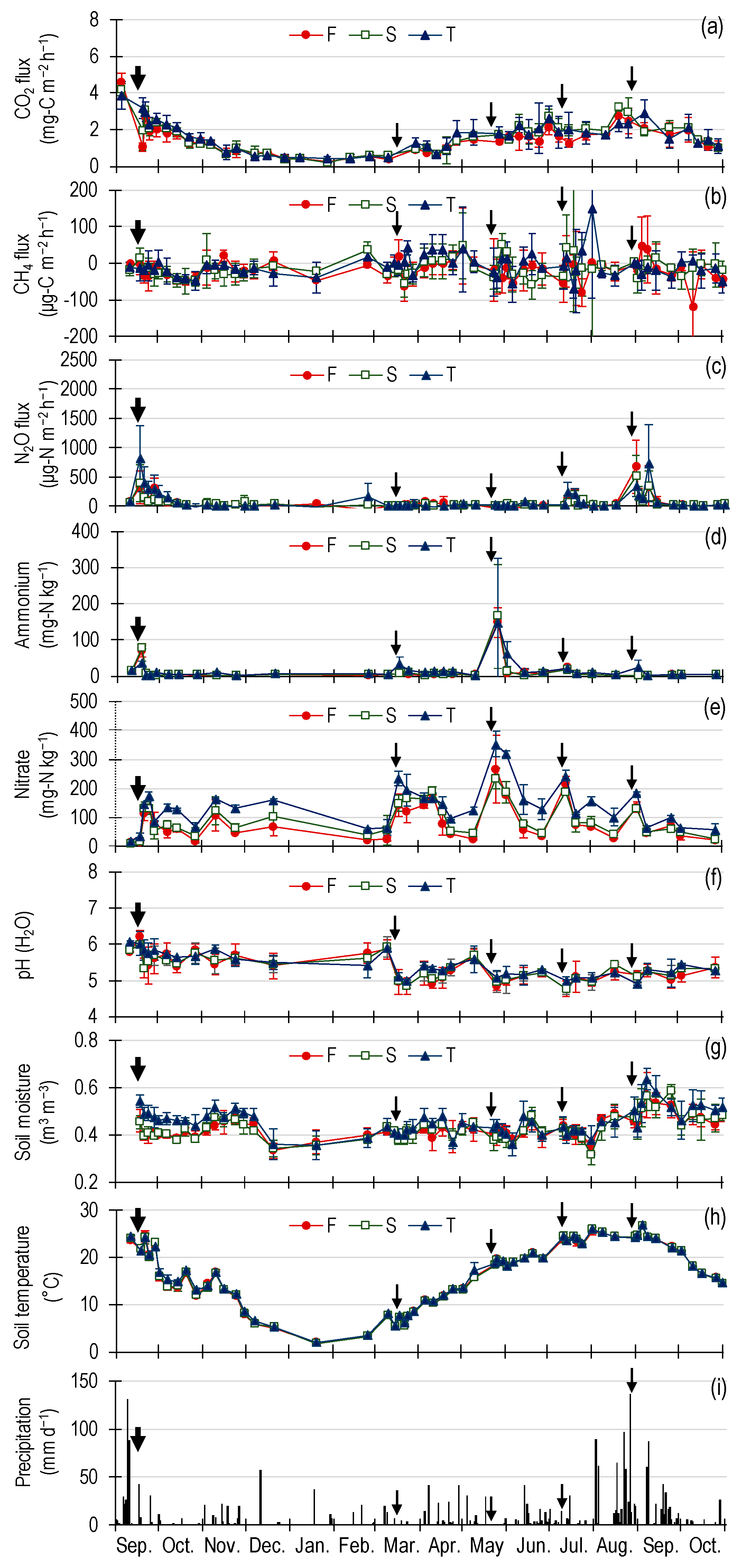
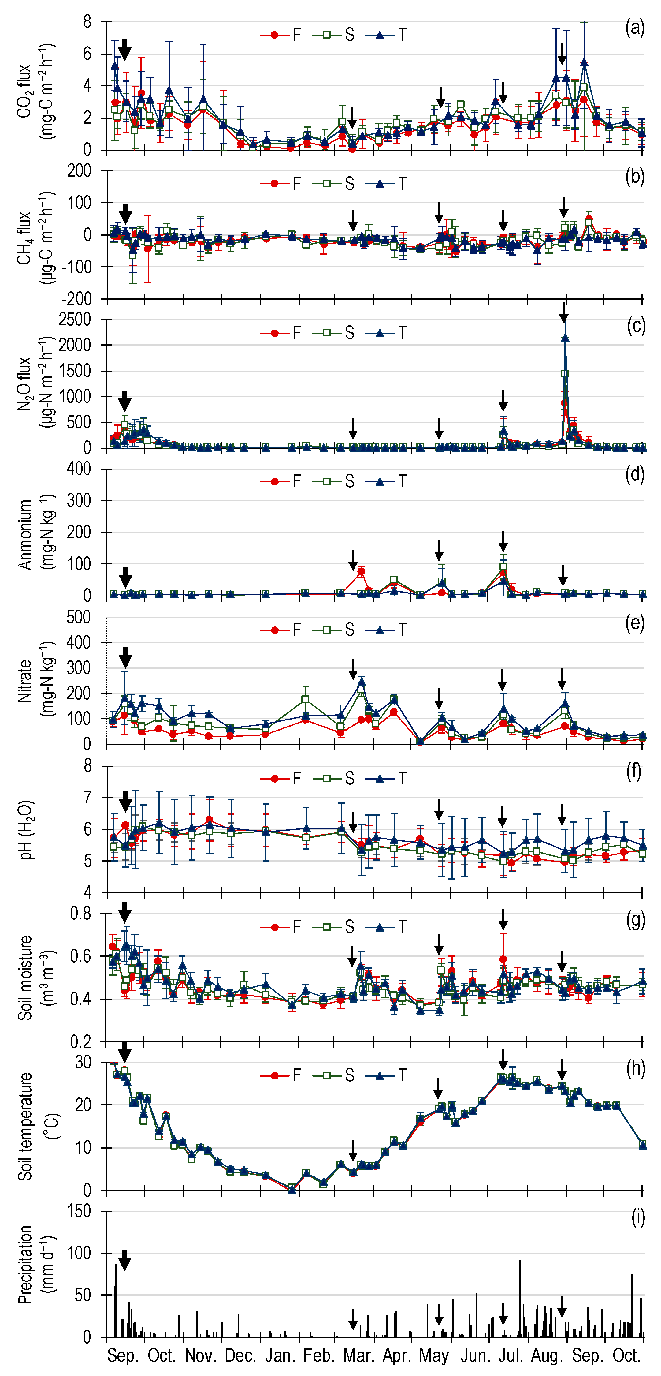
Statistical analyses were performed in Statistica v. 13.2 software (TIBCO Software Inc., Palo Alto, CA, USA). Two-way ANOVA was used to examine the effects of treatment (F, S, and T) and year (1 and 2) on the C balance, cumulative CH4 and N2O emissions, cumulative total herbage yield, cumulative N uptake, sum of GHG emissions, and GHGI. A p value less than 0.05 was considered statistically significant.

3. Results

3.1. Crop Residue

The quantity of C in crop residue in the topsoil did not differ significantly among plots (p = 0.921 in year 1 and p = 0.530 in year 2). Therefore, we used the average across treatments in each year in further calculations. The amount of C in crop residue in topsoil of renovated plots was 2.2 Mg-C ha−1 in year 1 and 2.4 Mg-C ha−1 in year 2.

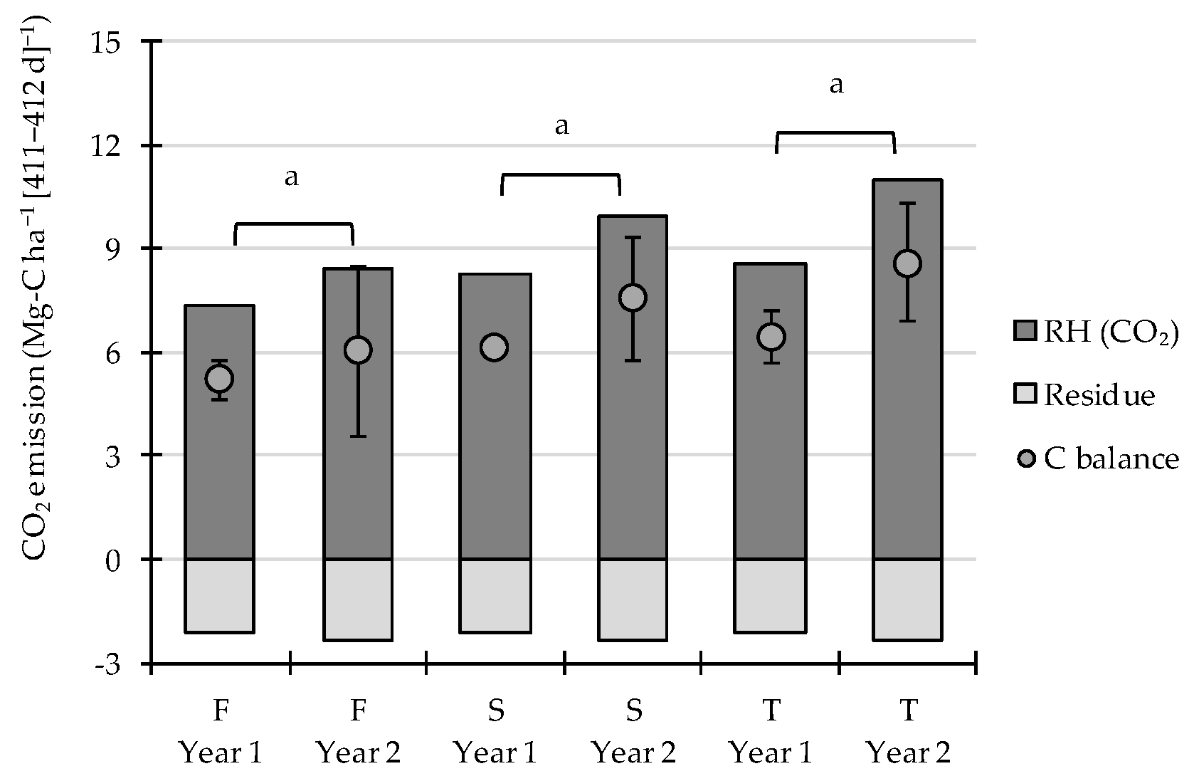
3.2. Heterotrophic Respiration, Cumulative CO2 Emission, and C Balance

The CO2 flux ranged from 0.2 to 4.6 mg-C m−2 h−1 in year 1 (Figure 1a) and from 0.0 to 5.5 mg-C m−2 h−1 in year 2 (Figure 2a). The CO2 flux increased as the soil temperature and soil moisture increased (p < 0.001 and p < 0.001).
Cumulative CO2 emissions ranged from 7.4 to 8.6 Mg-C ha−1 [412 d]−1 in year 1 and from 8.4 to 11.0 Mg-C ha−1 [411 d]−1 in year 2 (Figure 3). The C balance of grassland ranged from 5.2 to 6.4 Mg-C ha−1 [412 d]−1 in year 1 and from 6.0 to 8.6 Mg-C ha−1 [411 d]−1 in year 2, but there were no significant differences among the F, S, and T plots (Table 2).

3.3. Methane Flux and Cumulative Emission

The CH4 flux ranged from −118 to +148 µg-C m−2 h−1 in year 1 (Figure 1b) and from −66 to +49 µg-C m−2 h−1 in year 2 (Figure 2b). Note that negative values represent CH4 consumption in the soil. There was no significant correlation between soil temperature or moisture and CH4 flux (p = 0.330 and p = 0.161).
Cumulative CH4 emissions ranged from −1.9 to −0.9 kg-C ha−1 [412 d]−1 in year 1 and from −2.0 to −1.6 kg-C ha−1 [411 d]−1 in year 2 (Figure 4). The range of cumulative CH4 emissions was comparable to that previously observed in Japanese grasslands [17]. There were no significant differences among the F, S, and T plots (Table 3).

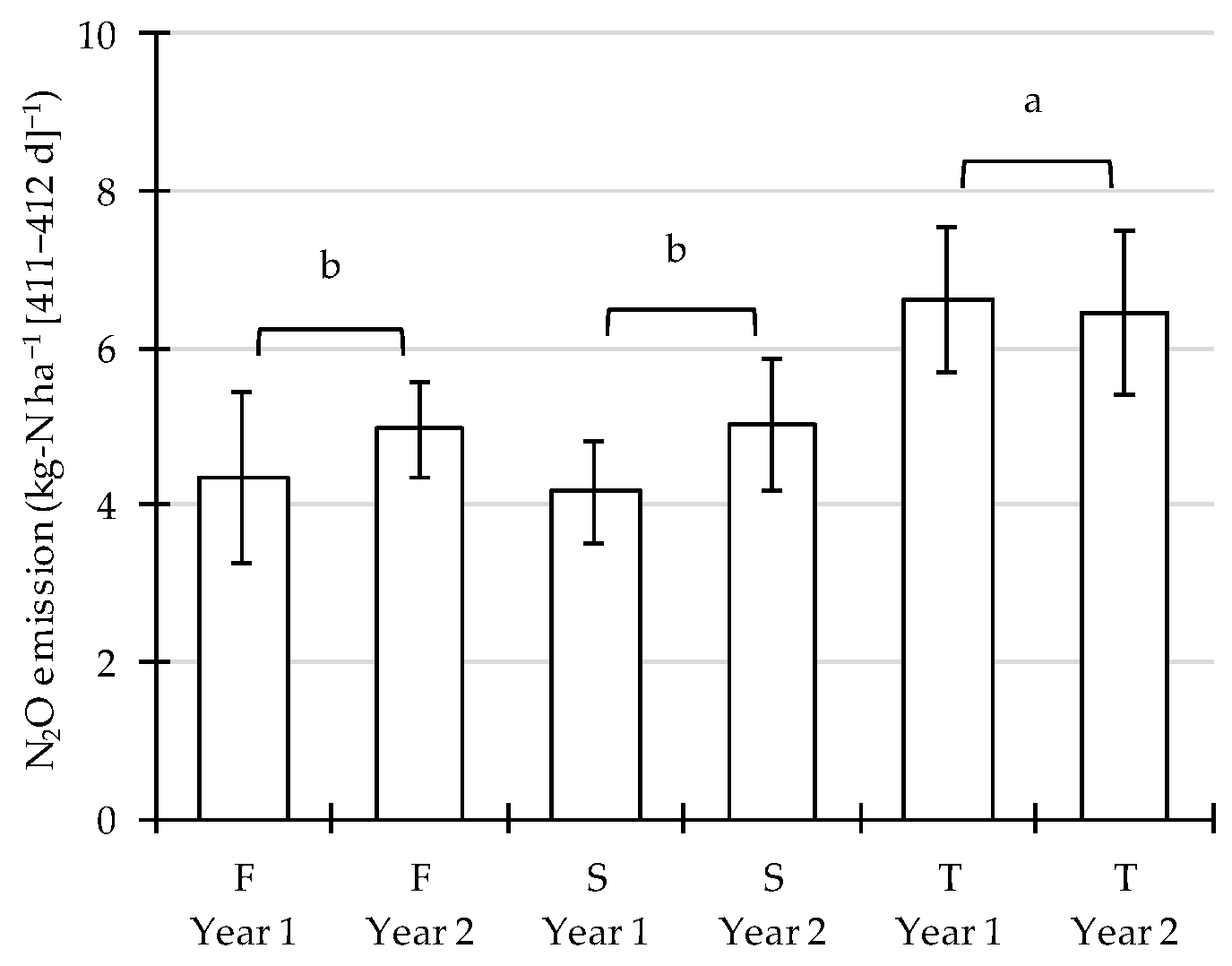
3.4. Nitrous Oxide Flux and Cumulative Emission

The N2O flux ranged from −62 to +810 µg-N m−2 h−1 in year 1 (Figure 1c) and from +1 to +2148 µg-N m−2 h−1 in year 2 (Figure 2c). Distinct N2O peaks were observed after renovation and fertilizations. The variation in N2O flux increased when the soil temperature was higher than 15 °C and the soil moisture was approximately 0.45 m3 m−3.
Cumulative N2O emissions ranged from 4.2 to 6.6 kg-N ha−1 [412 d]−1 in year 1 and from 5.0 to 6.4 kg-N ha−1 [411 d]−1 in year 2 (Figure 5). The range of cumulative N2O emissions was comparable to that previously observed in Japanese grasslands [17]. Cumulative N2O emission from F and S plots was smaller than that from T plots (Table 4).

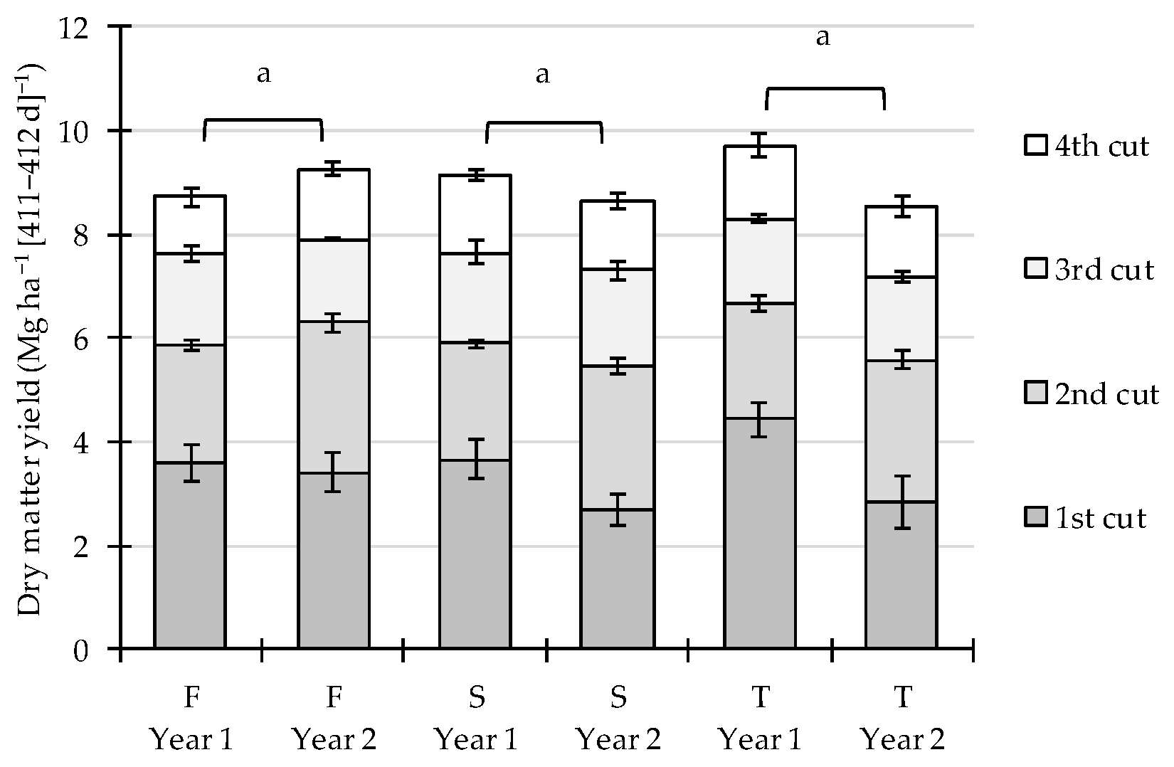
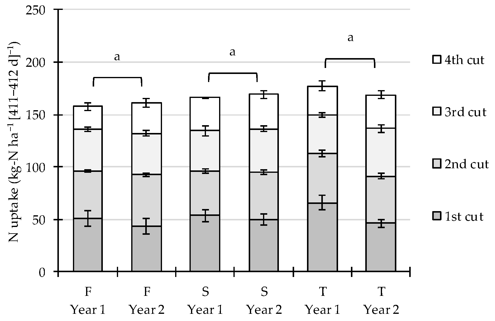
3.5. Herbage Yield and N Uptake by Harvest

The cumulative total herbage yield on a dry matter basis ranged from 8.7 to 9.7 Mg ha−1 [412 d]−1 in year 1 and from 8.5 to 9.3 Mg ha−1 [411 d]−1 in year 2 (Figure 6). The cumulative N uptake by harvest ranged from 158 to 177 kg-N ha−1 [412 d]−1 in year 1 and from 161 to 169 kg-N ha−1 [411 d]−1 in year 2 (Figure 7). The cumulative total herbage yield and N uptake by harvest of F, S, and T plots did not differ significantly (Table 5 and Table 6).

3.6. Soil Chemical Properties

Soil NH4–N concentration ranged from 1 to 165 mg-N kg−1 in year 1 (Figure 1d) and from 1 to 90 mg-N kg−1 in year 2 (Figure 2d). After renovation and fertilizations, NH4–N concentration temporarily increased. In both years, there were no significant differences among the F, S, and T plots.
Soil NO3–N concentration ranged from 13 to 353 mg-N kg−1 in year 1 (Figure 1e) and from 4 to 245 mg-N kg−1 in year 2 (Figure 2e). After renovation and fertilizations, NO3–N concentration temporarily increased. In year 1, NO3–N concentrations of F and S plots were lower than that of T plots. In year 2, NO3–N concentration of F plots was lower than that of S and T plots.
Soil pH (H2O) ranged from 4.8 to 6.2 in year 1 (Figure 1f) and from 4.9 to 6.3 in year 2 (Figure 2f). After renovation and fertilizations, pH (H2O) temporarily decreased. In year 1, there were no significant differences in soil pH (H2O) among the F, S, and T plots. In year 2, however, soil pH (H2O) in F and S plots were lower than that in T plots.

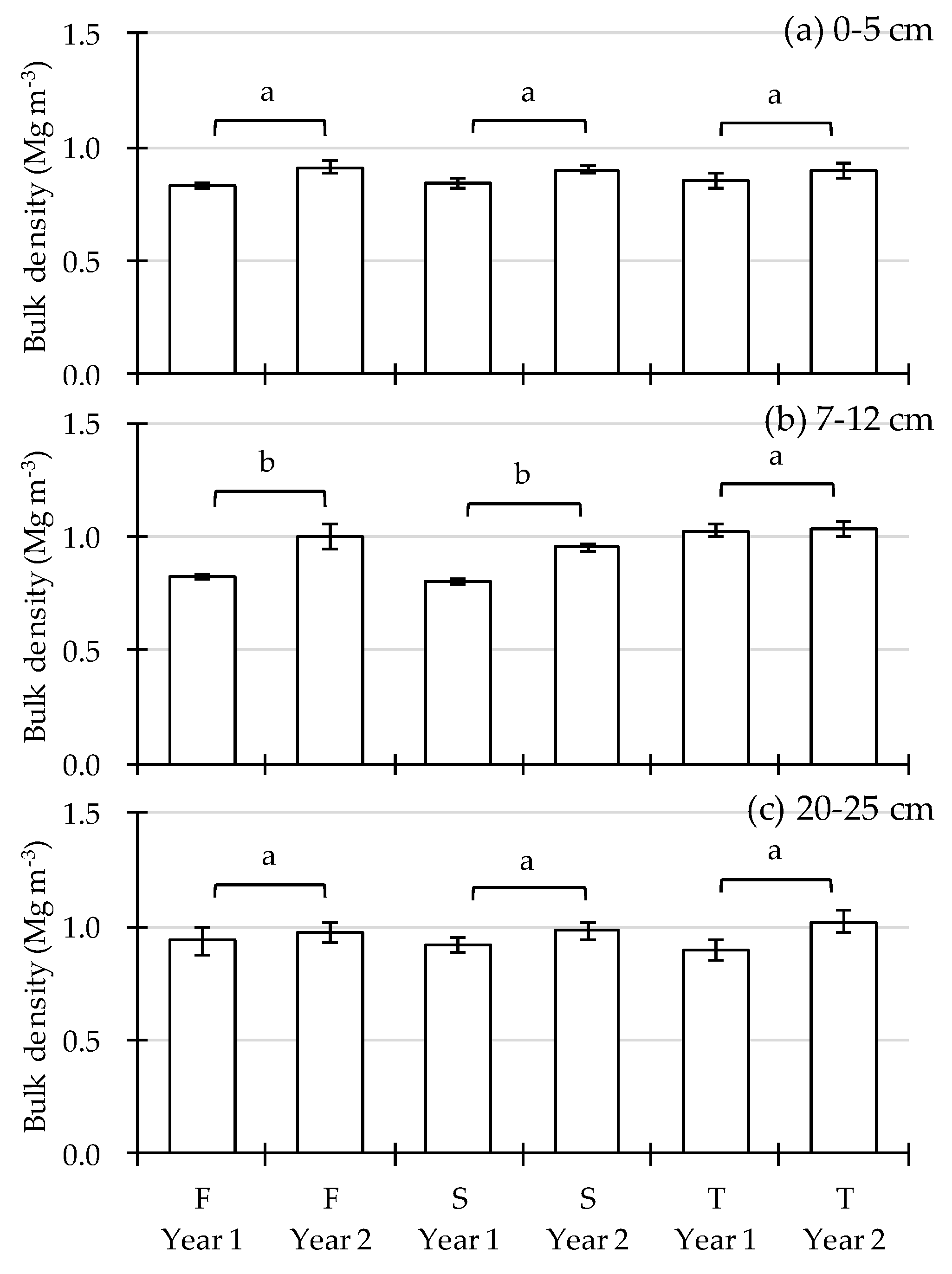
3.7. Soil Physical Properties

The bulk density of soils collected from the 0–5 cm layer ranged from 0.83 to 0.85 Mg m−3 in year 1 and from 0.90 to 0.91 Mg m−3 in year 2 (Figure 8a). That of soils collected from the 7–12 cm layer ranged from 0.81 to 1.03 Mg m−3 in year 1 and from 0.96 to 1.04 Mg m−3 in year 2 (Figure 8b). That of soils collected from the 20–25 cm layer ranged from 0.89 to 0.94 Mg m−3 in year 1 and from 0.97 to 1.02 Mg m−3 in year 2 (Figure 8c). Bulk densities of soils from the 0–5 and 20–25 cm layers did not differ significantly among the F, S, and T plots (Figure 8a,c). At 7–12 cm, however, bulk density was significantly greater in T plots than in F and S plots (Figure 8b). In the T plots, it was significantly greater at 20–25 cm than at 0–5 cm. Those of soils collected in year 1 were lower than those collected in year 2 (Table 7).
Soil moisture content ranged from 0.32 to 0.64 m3 m−3 in year 1 (Figure 1g) and from 0.35 to 0.65 m3 m−3 in year 2 (Figure 2g). In year 1, the soil moisture contents in the F and S plots were lower than those in T plots. In year 2, however, there were no significant differences among the F, S, and T plots.
In year 1, the lowest soil temperature (1.7 °C) was recorded on 20 January 2016 and the highest soil temperature (26.8 °C) was recorded on 5 September 2016 (Figure 1h). In year 2, the lowest soil temperature (0.0 °C) was recorded on 26 January 2017 and the highest soil temperature (28.1 °C) was recorded on 15 September 2016, the day following renovation (Figure 2h). In both years, there were no significant differences among the F, S, and T plots.

3.8. Precipitation

Cumulative precipitation was 1982 mm [412 d]−1 in year 1 (Figure 1i) and 1811 mm [411 d]−1 in year 2 (Figure 2i). In year 1, 42.5 mm d−1 of rain fell on the day following renovation (17 September 2015) and 42 mm [2 d]−1 of rain fell on the day of and the day following application of fertilizer for the 4th cut (29–30 August 2016). In year 2, 22.5 mm d−1 of rain fell during renovation (13 September 2016), 16.5 mm d−1 fell 3 days after renovation (17 September 2016), and 26 mm [2 d]−1 fell 2–3 days after application of fertilizer for the 4th cut (30–31 August 2017).

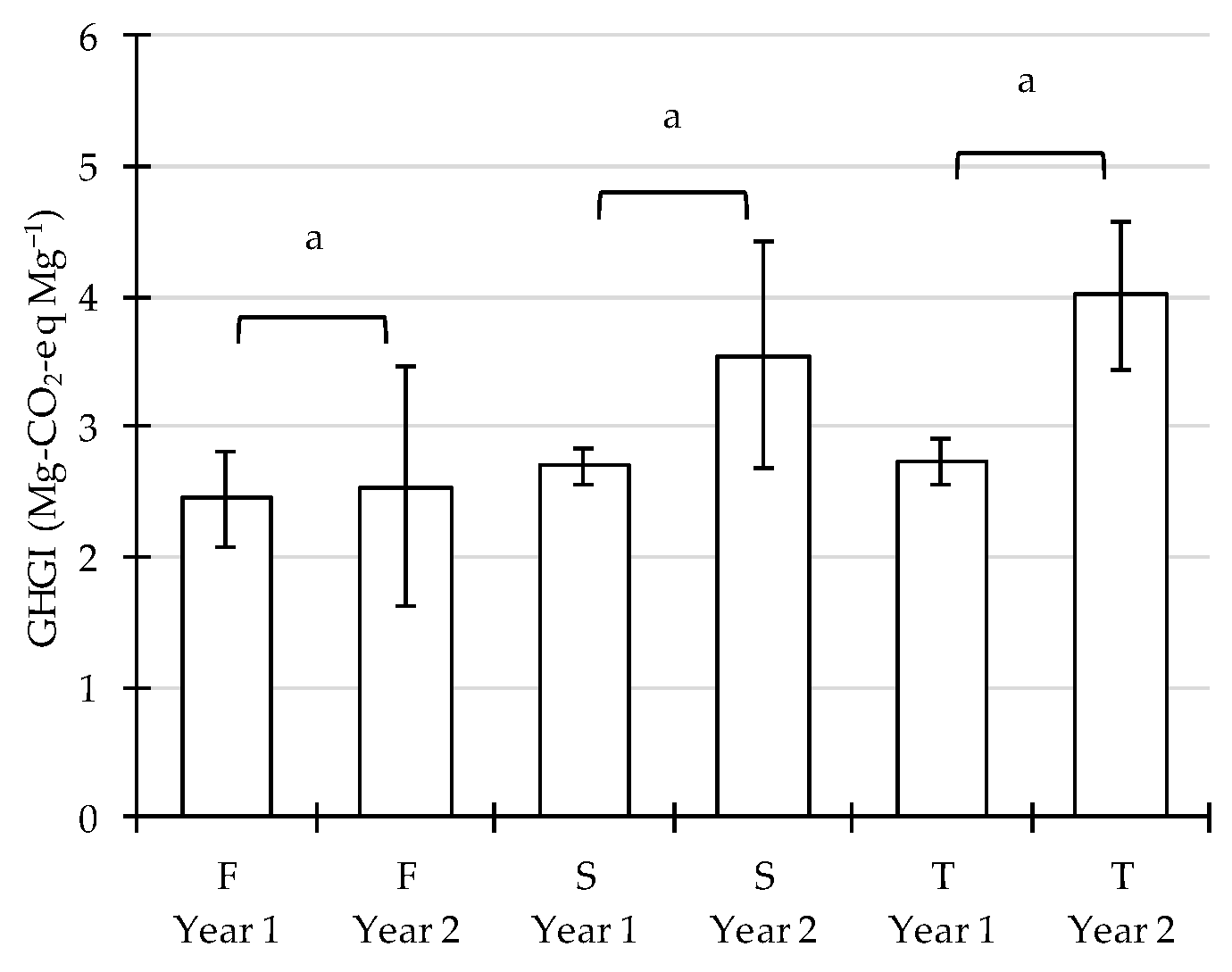
3.9. Sum of GHG Emissions and GHGI

The sum of GHG emissions ranged from 21.1 to 26.6 Mg–CO2-eq ha−1 [412 d]−1 in year 1 and from 24.4 to 34.5 Mg–CO2-eq ha−1 [411 d]−1 in year 2 (Figure 9). It decreased in the order of T > S > F plots, but F, S, and T plots did not differ significantly (Table 8).
The GHGI ranged from 2.4 to 2.7 Mg–CO2-eq Mg−1 in year 1 and from 2.5 to 4.0 Mg–CO2-eq Mg−1 in year 2 (Figure 10). The GHGI decreased in the order of T > S > F plots, but differences among plots were not significant (Table 9).

4. Discussion

4.1. Heterotrophic Respiration and C Balance

C input from crop residue is a key driver of soil organic C stocks [27]. During renovation, roots and stubble in previous grassland were killed and then supplied organic C to the soil in renovated grasslands. In both years, RH in F, S, and T plots (7.4–11.0 Mg–C ha−1 [411–412d]−1) was greater than the C input from crop residue (2.2–2.4 Mg-C ha−1), suggesting that organic C was lost to the atmosphere following renovation (Figure 3). This result agrees with our previous observation that in intensively managed cut grassland in Japan receiving only synthetic fertilizers, there is a net loss of C to the atmosphere [25].
Tillage disturbance results in disruption of soil aggregates, subsequently allows more contact between soil organic matter and soil microorganisms, then promotes decomposition of soil organic matter [28,29]. An initially higher O2 availability after soil disturbance will enhance the decay of the root C-pool, which before had a slower turnover [30]. Therefore, the conversion of grassland to cropland usually depletes soil organic C [31]. This may continue for a relatively long time before equilibrium conditions are reached [32].
In the present study, however, the F, S, and T plots showed no significant differences in C balance (Figure 3), suggesting that soil disturbance resulting from plowing and/or rotovating did not promote decomposition of soil organic C in our grasslands. This is probably because parts of the topsoil with substantial amounts of roots are buried into a deeper soil profile in the F and S plots and this might lead to a certain decrease in microbial activity and lower aeration [3]. In actual grasslands, a fast development of new sward after renovation can enhance photosynthesis and subsequent organic C supply to the soil. In this study, however, living vegetation was removed for measurement of heterotrophic respiration (see Section 2.4). From this viewpoint, the C balance in this study could be overestimated (Figure 3).
Conservation tillage, which minimizes disruption of soil aggregate structure, especially zero tillage, was reported to increase soil C sequestration [33], although the potential was revised downwards recently [34]. Long-term field experiments demonstrated that soil organic C accumulates near the surface under conservation tillage but accumulates deeper under conventional tillage, and that soil disturbance by tillage therefore has no significant effect on soil organic C stocks [27,35]. It has been pointed out that tillage itself may not reduce soil organic C stocks, but tillage without organic C application may reduce soil organic C stocks [36,37]. Since no till shows accumulation of soil C only on topsoil, occasional cultivation to bury the organic matter may enhance C sequestration at depth [38].
Soil moisture is another important driver of soil organic C stock. In Switzerland, ecosystem respiration was increased after plowing of a grassland in a pre-alpine lowland [10]. In Scotland and Canada, however, ecosystem or soil respiration was decreased after plowing of imperfectly drained grasslands [11,12]. In this present study, we observed a remarkable difference in soil moisture content among plots just after renovation, but not later (Figure 1g or Figure 2g). We infer that soil moisture content remained relatively unchanged, except immediately following renovation (Figure 1g or Figure 2g). Although the soil surface was compacted by both the Cambridge roller and tractor traffic for grassland management in the year following renovation, the soil of our grassland is derived from volcanic ash and is well drained [19].

4.2. CH4 and N2O Emissions

The surface soil moisture content tended to be lower in F and S plots than in T plots shortly after renovation, suggesting that plowing and/or rotovating increased aeration and evaporation in surface soil and so increased CH4 oxidation and decreased denitrification-derived N2O emission. Rainfall during the renovation treatment in year 2 increased the soil bulk density (Table 7, Figure 8) because high-moisture soil is easily compacted, leading to smaller differences in soil moisture content among plots in year 2 than in year 1.
Cumulative CH4 emissions were negative in both years and all the plots, suggesting that atmospheric CH4 was oxidized in the soil. A previous study showed that soil water decreased diffusion of CH4 and O2 in surface soil and inhibited CH4 oxidation [18]. We observed that plowing and/or rotovating temporarily increased aeration of surface soil, but there were no significant differences in cumulative CH4 emission among plots. This is probably because notable differences in soil moisture content among plots were of limited duration, i.e., just after renovation (Figure 1g or Figure 2g).
The NO3–N content of the top 5 cm of soil tended to be lower in F and S plots than in T plots, suggesting that plowing and/or rotovating reduced the amount available for denitrification in surface soil. In T plots, decomposing crop residue remaining on the soil surface released inorganic N and labile organic C, enriching denitrification sites in surface soil after rainfall and promoting N2O emission. In F and S plots, however, the crop residue was incorporated into a deeper soil profile, promoting complete reduction to N2 [16]. Suppression of N2O production in soil by mixing with glyphosate is another possible explanation [39].
After fertilizations in September (for renovation), July, and August, N2O flux peaks were greater than that in March and May (Figure 1c or Figure 2c). This is in line with a previous study suggesting that N2O emissions increased drastically when the average air temperature during a 12 day period after the N application exceeded 15 °C [14]. Rainfall pattern is another important factor controlling N2O emission. In both years, a substantial amount of rainfall just after fertilization in August promoted denitrification in surface soil, leading to higher N2O flux peaks in each year (Figure 1i or Figure 2i).
Cumulative N2O emissions were smaller in F and S plots than in T plots (Figure 5) partly due to the difference in N2O flux just after renovation (Figure 1c or Figure 2c). During the peak period of N2O flux just after renovation, the difference in soil moisture content among plots was larger than at any time point afterward (Figure 1g or Figure 2g). Crop residue remaining on the soil surface of T plots also promoted denitrification-derived N2O emission as was mentioned above.

4.3. Herbage Yield and N Uptake

Cumulative total herbage yield on a dry matter basis was within the standard range for the region (i.e., 8–10 Mg ha−1 y−1). There were no significant difference in cumulative total herbage yield and N uptake in F, S, and T plots, suggesting that all three methods of renovation worked well by ensuring a fast establishment of good swards (Figure 6 and Figure 7).

4.4. Sum of GHG Emissions and GHGI

Cumulative emissions contributed 8%–12% of N2O, almost 0% of CH4 and 88%–92% of CO2 (i.e., C balance) to their sum (Figure 9), suggesting that C balance is the main driver. C input from crop residue was insufficient to compensate for the loss, via heterotrophic respiration, of organic C in cut grasslands (Figure 3). Cumulative N2O emissions were smaller from F and S plots than from T plots (Figure 5), however, the method of renovation did not change the sum of GHG emissions or GHGI, probably because C balance did not differ significantly among plots (Figure 3).
Our previous study demonstrated that annual application of farmyard manure is essential to increase soil organic C in cut grasslands in Japan [25]. A recent survey reported that in Hokkaido and in other prefectures in Japan, farmyard manure is applied as a basal fertilizer for renovation at rates of 136 and 105 Mg ha−1 (fresh matter basis), respectively [7]. These amounts are more than 3 times the recommended annual rate of application for a grassland during the maintenance (unrenovated) phase. It has been pointed out that combination of organic matter application and occasional tillage could increase the rate of organic C accumulation [37]. Therefore, application of farmyard manure during renovation could be important to compensate for the loss of organic C and to reduce GHG emissions from cut grasslands in Japan.

5. Conclusions

Cumulative total herbage yields of the F, S, and T plots did not differ significantly from each other. Cumulative N2O emissions from F and S plots were significantly smaller than that from T plots, however, there were no significant differences in the sum of GHG emissions (i.e., C balance plus cumulative CH4 and N2O emissions) among F, S, and T plots. Consequently, GHGI—i.e., the sum of GHG emissions per cumulative total herbage yield—did not differ significantly among F, S, and T plots.

Funding

This work was financially supported by the Ministry of Agriculture, Forestry and Fisheries, Japan, through a research project entitled “Development of Agricultural Production Technologies for Adaptation to Global Warming”.

Acknowledgments

I would like to thank Ryusuke Hatano at Hokkaido University, Arata Nagatake at Civil Engineering Research Institute for Cold Region, Shoji Matsuura at National Agriculture and Food Research Organization for useful discussions, sample analyses, and data collections.

Conflicts of Interest

The author declares no conflict of interest. The funding body had no role in the collection, analyses, or interpretation of data, in the writing of the manuscript, or in the decision to publish the results.

References

  1. Deguchi, K. Invasion of rhizomatous grasses on timothy grassland in Hokkaido. Jpn. J. Grassl. Sci. 2016, 62, 153–157. (In Japanese) [Google Scholar]
  2. Hojito, M. Studies on grassland acidification caused by fertilizer application and its effects on grass growth. Rep. Hokkaido Prefect. Agric. Exp. Stn. 1994, 83, 1–109, (In Japanese with English Summary). [Google Scholar]
  3. Kayser, M.; Müller, J.; Isselstein, J. Grassland renovation has important consequences for C and N cycling and losses. Food Energy Secur. 2018, 7, e00146. [Google Scholar] [CrossRef]
  4. MAFF (Ministry of Agriculture, Forestry and Fisheries). Grassland Management Guidelines: Grassland Maintenance Edition; MAFF: Tokyo, Japan, 2006; pp. 1–189.
  5. Tarumi, E.; Tsuiki, M.; Mori, A. Evaluation of global warming effects to cool season grass productivity with models. J. Jpn. Agric. Sys. Soc. 2018, 34, 7–15, (In Japanese with English Summary). [Google Scholar]
  6. Otsuka, H. Finding the path from grass improvement project in Hokkaido. Jpn. J. Grassl. Sci. 2016, 62, 163–167. (In Japanese) [Google Scholar]
  7. Hatano, R. Report of Survey on Actual Management of Grassland and Forage Cropping Areas in Japan; Hokkaido University: Sapporo, Japan, 2017; pp. 1–56. [Google Scholar]
  8. Six, J.; Feller, C.; Denef, K.; Ogle, S.; de Sa Moraes, J.C.; Albrecht, A. Soil organic matter, biota and aggregation in temperate and tropical soils—Effects of no-tillage. Agronomie 2002, 22, 755–775. [Google Scholar] [CrossRef] [Green Version]
  9. Baker, J.M.; Ochsner, T.E.; Venterea, R.T.; Griffis, T.J. Tillage and soil carbon sequestration—What do we really know? Agric. Ecosyst. Environ. 2007, 118, 1–5. [Google Scholar] [CrossRef]
  10. Merbold, L.; Eugster, W.; Stieger, J.; Zahniser, M.; Nelson, D.; Buchmann, N. Greenhouse gas budget (CO2, CH4 and N2O) of intensively managed grassland following restoration. Glob. Chang. Biol. 2014, 20, 1913–1928. [Google Scholar] [CrossRef]
  11. Drewer, J.; Anderson, M.; Levy, P.; Scholtes, B.; Helfter, C.; Parker, J.; Rees, R.M.; Skiba, U.M. The impact of ploughing intensively managed temperate grasslands on N2O, CH4 and CO2 fluxes. Plant Soil 2017, 411, 193–208. [Google Scholar] [CrossRef]
  12. MacDonald, J.D.; Angers, D.A.; Rochette, P.; Chantigny, M.H.; Royer, I.; Gasser, M. Plowing a poorly drained grassland reduced soil respiration. Soil Sci. Soc. Am. J. 2010, 74, 2067–2076. [Google Scholar] [CrossRef]
  13. Mori, A.; Hojito, M. Grassland renovation increases N2O emission from a volcanic grassland soil in Nasu, Japan. Soil Sci. Plant Nutr. 2007, 53, 812–818. [Google Scholar] [CrossRef] [Green Version]
  14. Mori, A.; Hojito, M. Effect of combined application of manure and fertilizer on N2O fluxes from a grassland soil in Nasu, Japan. Agric. Ecosyst. Environ. 2012, 160, 40–50. [Google Scholar] [CrossRef]
  15. Velthof, G.L.; Hoving, I.E.; Dolfing, J.; Smit, A.; Kuikman, P.J.; Oenema, O. Method and timing of grassland renovation affects herbage yield, nitrate leaching, and nitrous oxide emission in intensively managed grasslands. Nutr. Cycl. Agroecosyst. 2010, 86, 401–412. [Google Scholar] [CrossRef] [Green Version]
  16. MacDonald, J.D.; Rochette, P.; Chantigny, M.H.; Angers, D.A.; Royer, I.; Gasser, M.O. Ploughing a poorly drained grassland reduced N2O emissions compared to chemical fallow. Soil Tillage Res. 2011, 111, 123–132. [Google Scholar] [CrossRef]
  17. Shimizu, M.; Hatano, R.; Arita, T.; Kouda, Y.; Mori, A.; Matsuura, S.; Niimi, M.; Jin, T.; Desyatkin, A.R.; Kawamura, O.; et al. The effect of fertilizer and manure application on CH4 and N2O emissions from managed grasslands in Japan. Soil Sci. Plant Nutr. 2013, 59, 69–86. [Google Scholar] [CrossRef] [Green Version]
  18. Mori, A.; Hojito, M.; Kondo, H.; Matsunami, H.; Scholefield, D. Effects of plant species on CH4 and N2O fluxes from a volcanic soil in Nasu, Japan. Soil Sci. Plant Nutr. 2005, 51, 19–27. [Google Scholar] [CrossRef]
  19. Kurashima, K.; Ota, T.; Kusaba, T.; Amano, Y.; Yamamoto, K.; Kimura, T.; Kondo, H.; Saito, G. Classification and characteristics of soils at the National Grassland Research Institute. Misc. Publ. Natl. Grassl. Res. Inst. 1993, 3, 1–47. (In Japanese) [Google Scholar]
  20. Soil Survey Staff. Keys to Soil Taxonomy, 12th ed.; USA Natural Resources Conservation Service: Washington, DC, USA, 2014; pp. 1–360.
  21. Matsuura, S.; Nakao, S.; Hojito, M. Short-term effects of grassland renovation on CO2 exchange of grasslands in a temperate humid region. J. Agric. Meteorol. 2017, 73, 174–186. [Google Scholar] [CrossRef] [Green Version]
  22. Hanson, P.J.; Edwards, N.T.; Garten, C.T.; Andrews, J.A. Separating root and soil microbial contributions to soil respiration: A review of methods and observations. Biogeochemistry 2000, 48, 115–146. [Google Scholar] [CrossRef]
  23. Mori, A.; Hojito, M. Effect of dairy manure type on the carbon balance of mowed grassland in Nasu, Japan: Comparison between manure slurry plus synthetic fertilizer plots and farmyard manure plus synthetic fertilizer plots. Soil Sci. Plant Nutr. 2015, 61, 736–746. [Google Scholar] [CrossRef] [Green Version]
  24. Mori, A.; Hojito, M. Effect of dairy manure type and supplemental synthetic fertilizer on methane and nitrous oxide emissions from a grassland in Nasu, Japan. Soil Sci. Plant Nutr. 2015, 61, 347–358. [Google Scholar] [CrossRef] [Green Version]
  25. Hirata, R.; Miyata, A.; Mano, M.; Shimizu, M.; Arita, T.; Kouda, Y.; Matsuura, S.; Niimi, M.; Mori, A.; Saigusa, T.; et al. Carbon dioxide exchange at four intensively managed grassland sites across different climate zones of Japan and the influence of manure application on ecosystem carbon and greenhouse gas budgets. Agric. For. Meteorol. 2013, 177, 57–68. [Google Scholar] [CrossRef]
  26. Intergovernmental Panel Climate Change. Climate Change 2007: The Physical Science Basis, Contribution of Working Group I to the Fourth Assessment Report of the Intergovernmental Panel on Climate Change; Solomon, S., Qin, D., Manning, M., Chen, Z., Marquis, M., Averyt, K.B., Tignor, M., Miller, H.L., Eds.; Cambridge University Press: Cambridge, UK, 2007. [Google Scholar]
  27. Dimassi, B.; Mary, B.; Wylleman, R.; Labreuche, J.; Couture, D.; Piraux, F.; Cohan, J.P. Long-term effect of contrasted tillage and crop management on soil carbon dynamics during 41 years. Agric. Ecosyst. Environ. 2014, 188, 134–146. [Google Scholar] [CrossRef]
  28. Lal, R. Soil carbon sequestration to mitigate climate change. Geoderma 2004, 123, 1–22. [Google Scholar] [CrossRef]
  29. Reinsch, T.; Loges, R.; Kluß, C.; Taube, F. Renovation and conversion of permanent grass-clover swards to pasture or crops: Effects on annual N2O emissions in the year after ploughing. Soil Tillage Res. 2018, 175, 119–129. [Google Scholar] [CrossRef]
  30. Dietzel, R.; Liebman, M.; Archontoulis, S. A deeper look at the relationship between root carbon pools and the vertical distribution of the soil carbon pool. Soil 2017, 3, 139–152. [Google Scholar] [CrossRef] [Green Version]
  31. Deng, L.; Zhu, G.; Tang, Z.; Shangguan, Z. Global patterns of the effects of land-use changes on soil carbon stocks. Glob. Ecol. Conserv. 2016, 5, 127–138. [Google Scholar] [CrossRef] [Green Version]
  32. Vellinga, T.; van den Pol-van Dasselaar, A.; Kuikman, P. The impact of grassland ploughing on CO2 and N2O emissions in the Netherlands. Nutr. Cycl. Agroecosyst. 2004, 70, 33–45. [Google Scholar] [CrossRef]
  33. Six, J.; Elliott, E.T.; Paustian, K. Soil macroaggregate turnover and microaggregate formation: A mechanism for C sequestration under no-tillage agriculture. Soil Biol. Biochem. 2000, 32, 2099–2103. [Google Scholar] [CrossRef]
  34. Paustian, K.; Lehmann, J.; Ogle, S.; Reay, D.; Robertson, G.P.; Smith, P. Climate-smart soils. Nature 2016, 532, 49–57. [Google Scholar] [CrossRef] [Green Version]
  35. Gál, A.; Vyn, T.J.; Michéli, E.; Kladivko, E.J.; McFee, W.W. Soil carbon and nitrogen accumulation with long-term no-till versus moldboard plowing overestimated with tilled-zone sampling depths. Soil Tillage Res. 2007, 96, 42–51. [Google Scholar] [CrossRef]
  36. Dalal, R.C.; Allen, D.E.; Wang, W.J.; Reeves, S.; Gibson, I. Organic carbon and total nitrogen stocks in a Vertisol following 40 years of no-tillage, crop residue retention and nitrogen fertilization. Soil Tillage Res. 2011, 112, 133–139. [Google Scholar] [CrossRef]
  37. Mukumbuta, I.; Hatano, R. Do tillage and conversion of grassland to cropland always deplete soil organic carbon? Soil Sci. Plant Nutr. 2019, 66, 1–8. [Google Scholar] [CrossRef]
  38. Minasny, B.; Malone, B.P.; McBratney, A.B.; Angers, D.A.; Arrouays, D.; Chambers, A.; Chaplot, V.; Chen, Z.S.; Cheng, K.; Das, B.S.; et al. Soil carbon 4 per mile. Geoderma 2017, 292, 59–86. [Google Scholar] [CrossRef]
  39. Kyaw, K.M.; Toyota, K. Suppression of nitrous oxide production by the herbicides glyphosate and propanil in soils supplied with organic matter. Soil Sci. Plant Nutr. 2007, 53, 441–447. [Google Scholar] [CrossRef]
Figure 1. (a) CO2, (b) CH4, and (c) N2O fluxes from grassland plots; (d) ammonium, (e) nitrate, (f) pH, (g) moisture, and (h) temperature in the soil; and (i) precipitation during year 1 (12 September 2015 to 28 October 2016). F, full inversion tillage; S, shallow tillage; T, a tine drill. Arrows indicate the timing of ⬇ renovation and ↓ synthetic fertilizer application. Whiskers represent standard error (n = 4 for gas fluxes and soil physical properties; n = 2 for soil chemical properties).
Agriculture 10 00031 g001
Figure 2. (a) CO2, (b) CH4, and (c) N2O fluxes from grassland plots; (d) ammonium, (e) nitrate, (f) pH, (g) moisture, and (h) temperature in the soil; and (i) precipitation during year 2 (12 September 2016 to 28 October 2017). F, full inversion tillage; S, shallow tillage; T, a tine drill. Arrows indicate the timing of ⬇ renovation and ↓ synthetic fertilizer application. Whiskers represent standard error (n = 4 for gas fluxes and soil physical properties; n = 2 for soil chemical properties).
Agriculture 10 00031 g002
Figure 3. C balance of grassland plots renovated using full inversion tillage (F), shallow tillage (S), or a tine drill (T). RH is the amount of heterotrophic respiration. Whiskers represent standard error (n = 4). Bars that are linked with the same letter are not significantly different.
Agriculture 10 00031 g003
Figure 4. Cumulative CH4 emissions from grassland plots renovated using full inversion tillage (F), shallow tillage (S), or a tine drill (T). Whiskers represent standard error (n = 4). Bars that are linked with the same letter are not significantly different.
Agriculture 10 00031 g004
Figure 5. Cumulative N2O emissions from grassland plots renovated using full inversion tillage (F), shallow tillage (S), or a tine drill (T). Whiskers represent standard error (n = 4). Bars that were linked with the same letter are not significantly different.
Agriculture 10 00031 g005
Figure 6. Dry matter yields of grassland plots renovated using full inversion tillage (F), shallow tillage (S), or a tine drill (T). Whiskers represent standard error (n = 4). Bars that are linked with the same letter are not significantly different.
Agriculture 10 00031 g006
Figure 7. N uptake in grassland plots renovated using full inversion tillage (F), shallow tillage (S), or a tine drill (T). Whiskers represent standard error (n = 4). Bars that are linked with the same letter are not significantly different.
Agriculture 10 00031 g007
Figure 8. Depth profiles of bulk densities of soils collected from (a) 0–5, (b) 7–12 and (c) 20–25 cm in grassland plots renovated using full inversion tillage (F), shallow tillage (S) or a tine drill (T). Whiskers represent standard error (n = 4). Bars that are linked with the same letter are not significantly different.
Agriculture 10 00031 g008
Figure 9. Sum of greenhouse gas (GHG) emissions of grassland plots renovated with full inversion tillage (F), shallow tillage (S), or a tine drill (T). Whiskers represent standard error (n = 4). Bars that are linked with the same letter are not significantly different.
Agriculture 10 00031 g009
Figure 10. Greenhouse gas intensity (GHGI) of grassland plots renovated using full inversion tillage (F), shallow tillage (S), or a tine drill (T). Whiskers represent standard error (n = 4). Bars that are linked with the same letter are not significantly different.
Agriculture 10 00031 g010
Table 1. Application rates of synthetic N, P, and K fertilizers.
Year 1 (12 September 2015 to 28 October 2016)
RenovationMaintenance
15–16 September
2015
15 March
2016
23 May
2016
11 July
2016
29 August
2016
N (kg-N ha−1)4060505030
P (kg-P2O5 ha−1)20030252515
K (kg-K2O ha−1)8060505030
Year 2 (12 September 2016 to 28 October 2017)
RenovationMaintenance
12–14 September
2016
15 March 201722 May
2017
11 July
2017
28 August
2017
N (kg-N ha−1)4060505030
P (kg-P2O5 ha−1)20030252515
K (kg-K2O ha−1)8060505030
Table 2. ANOVA results for C balance of grassland.
FactorSSdfMSFp Value
Treatment197.7298.90.6460.541
Year172.71172.71.1290.309
Treatment × Year24.1212.10.0790.925
SS, sum of squares; df, degrees of freedom; and MS, mean square.
Table 3. ANOVA results for cumulative CH4 emissions from grasslands.
FactorSSdfMSFp Value
Treatment0.00220.0011.2430.323
Year0.00110.0012.0070.182
Treatment × Year0.00120.0000.5870.571
SS, sum of squares; df, degrees of freedom; and MS, mean square.
Table 4. ANOVA results for cumulative N2O emissions from grasslands.
FactorSSdfMSFp Value
Treatment4.22922.1143.5710.061
Year0.25110.2510.4230.528
Treatment × Year0.25920.1300.2190.806
SS, sum of squares; df, degrees of freedom; and MS, mean square.
Table 5. ANOVA results for dry matter yield.
FactorSSdfMSFp Value
Treatment0.23920.1200.1320.878
Year0.85210.8520.9370.352
Treatment × Year3.01021.5051.6550.232
SS, sum of squares; df, degrees of freedom; and MS, mean square.
Table 6. ANOVA results for N uptake by harvested grass.
FactorSSdfMSFp Value
Treatment40422020.6580.536
Year2120.0060.939
Treatment × Year64223211.0460.381
SS, sum of squares; df, degrees of freedom; and MS, mean square.
Table 7. ANOVA results for soil bulk density.
FactorSSdfMSFp Value
Treatment0.04120.0203.7000.034
Year0.12910.12923.520<0.001
Depth0.09720.0488.8300.001
Treatment × Year0.00420.0020.4100.668
Treatment × Depth0.06340.0162.8600.037
Year × Depth0.00820.0040.7300.489
SS, sum of squares; df, degrees of freedom; and MS, mean square.
Table 8. ANOVA results for sum of greenhouse gas (GHG) emissions in grasslands.
FactorSSdfMSFp Value
Treatment246.82123.40.7710.484
Year185.11185.11.1570.303
Treatment × Year20.3210.20.0630.939
SS, sum of squares; df, degrees of freedom; and MS, mean square.
Table 9. ANOVA results for greenhouse gas intensity (GHGI).
FactorSSdfMSFp Value
Treatment3.23121.6150.9970.398
Year3.30513.3052.0390.179
Treatment × Year1.44420.7220.4450.651
SS, sum of squares; df, degrees of freedom; and MS, mean square.

